Technical note: Challenges in detecting free tropospheric ozone trends in a sparsely sampled environment

High-quality long-term observational records are essential to ensure appropriate and reliable trend detection of tropospheric ozone. However, the necessity of maintaining high sampling frequency, in addition to continuity, is often under-appreciated. A common assumption is that, so long as long-term records (e.g., a span of a few decades) are available, (1) the estimated trends are accurate and precise, and (2) the impact of small-scale variability (e.g., weather) can be eliminated. In this study, we show that the undercoverage bias (e.g., a type of sampling error resulting from statistical inference based on sparse or insufficient samples, such as once-per-week sampling frequency) can persistently reduce the trend accuracy of free tropospheric ozone, even if multi-decadal time series are considered. We use over 40 years of nighttime ozone observations measured at Mauna Loa, Hawaii (representative of the lower free troposphere), to make this demonstration and quantify the bias in monthly means and trends under different sampling strategies. We also show that short-term meteorological variability remains a cause of an inflated long-term trend uncertainty. To improve the trend precision and accuracy due to sampling bias, two remedies are proposed: (1) a data variability attribution of colocated meteorological influence can efficiently reduce estimation uncertainty and moderately reduce the impact of sparse sampling, and (2) an adaptive sampling strategy based on anomaly detection enables us to greatly reduce the sampling bias and produce more accurate trends using fewer samples compared to an intense regular sampling strategy.

1 Introduction

Tropospheric ozone is the third most important greenhouse gas (after carbon dioxide and methane, Gulev et al., 2021). Ozone is also a surface pollutant detrimental to human health and crop productivity (Fleming et al., 2018; Mills et al., 2018). The lifetime of tropospheric ozone ranges from minutes in the boundary layer to roughly 3 weeks for a global average (Young et al., 2013), and its sources include photochemical production from various precursor gases and stratosphere–troposphere exchange, which is challenging to accurately quantify because emissions of ozone precursor gases, atmospheric transport pathways, and extreme weather patterns also change over time (Stohl et al., 2003; Zhang et al., 2016). While the observations from remote high elevation sites can be used to quantify regional-scale ozone trends and variability within the planetary boundary layer or lower free troposphere (Cooper et al., 2020), only sparse profiles from ozonesondes, lidars, or aircraft are available to monitor ozone in the middle or upper troposphere.

Trend detection of free tropospheric ozone at a global scale is particularly challenging because ozone is highly dynamic, and observations are too limited (infrequent in time and sparse in space). In terms of long-term observations, ozonesonde and aircraft provide high-quality ozone observations throughout the depth of the troposphere with a fine vertical resolution, but these programs are expensive to maintain, and sampling rates are often quite low. Within the global ozonesonde network (Tarasick et al., 2019), only three sites – Hohenpeissenberg (Germany, 1966 to present), Payerne (Switzerland, 1968 to present), and Uccle (Belgium, 1969 to present) – manage to launch ozonesondes with a sampling frequency of two or three times a week. Even so, consistent long-term free tropospheric trends cannot be found between these three western European sites in relatively close proximity (Chang et al., 2022). While most of the other ozonesonde sites target a once-per-week sampling frequency, the actual sampling rate is often less (e.g., the NOAA Global Monitoring Laboratory (GML) ozonesonde record in American Samoa has an average sampling rate of 35 profiles per year); therefore, the precision and accuracy of trends estimated from these time series might be even less reliable. Of the other instruments, only the lidar operated at the Jet Propulsion Laboratory Table Mountain Facility (California) has managed to provide ozone profiles with varying frequencies of two to five times a week since 1999 (Chouza et al., 2019).

The IAGOS (In-Service Aircraft for a Global Observing System) program is also an important source of tropospheric ozone observations. Since 1994, IAGOS commercial aircraft have provided ozone profiles worldwide, and because the program's ozone instruments are calibrated regularly, its observational record can be considered to be a reference data set (Tarasick et al., 2019). Nevertheless, from a sampling point of view, since the availability of IAGOS data is tied to pre-determined flight schedules, the sampling schemes are often irregular and intermittent. Western Europe is the only region with abundant and near-continuous ozone measurements dating from 1994, with an average of more than 100 profiles per month (mostly from Frankfurt, Paris, Munich, Brussels, Düsseldorf, and Amsterdam). The IAGOS observations collected at other regions often have data gaps (several years in some cases); therefore, the reliability of trend estimates based on these time series might be subject to higher levels of uncertainty.

With the exceptions discussed above, free tropospheric ozone observations are either sparse in time (once-per-week sampling) or intermittent. However, these free tropospheric vertical profiles are still the only long-term observational records available to validate satellite data and global chemistry–climate model simulations. The common approach to compare satellite data to in situ or ground-based observations is to spatially and temporally co-locate comparisons between each individual profile and the corresponding satellite value (Zhang et al., 2010) or at a monthly aggregated scale (Ziemke et al., 2006). This study shows that the sampling errors (due to a sparse sampling frequency) might persistently bias the trend estimate even if multi-decadal records are considered. Therefore, the implication is that inconsistent trends can exist between ground-based and satellite observations due to different sampling schemes.

In terms of the impact of sampling on tropospheric ozone monthly means, Logan (1999) analyzed ozonesonde profile data and suggested that at least 20 profiles are required to maintain the 2σ range below ± 30 % of the monthly means near the extratropical tropopause and below ± 15 % of the monthly means for the tropical and extratropical free troposphere. Using the IAGOS commercial aircraft profiles above Frankfurt, Saunois et al. (2012) evaluated the sampling uncertainty on seasonal means at 100 hPa vertical resolution and found the uncertainty to be around 10 % at 700–500 hPa and around 15 % at 400 hPa for a sampling frequency of four profiles per month. However, the uncertainty can be reduced to 5 % and 8 %, respectively, if the sampling frequency is increased to 12 profiles per month. Cooper et al. (2010) merged all April–May ozone profiles (all available ozonesonde, lidar, and aircraft measurements) above western North America to show that ozone had increased in the free troposphere over 1995–2008 and determined that 50 profiles per April–May season (or 25 profiles per month) are required to produce a seasonal column mean value in the 3–8 km range within ± 2 % bias.

In terms of the impact of sampling frequency on tropospheric ozone trends, by using the IAGOS profiles above western Europe, where the trend values are around 1–2 ppbv per decade for 950–400 hPa and between 2–9 ppbv per decade for 350–250 hPa over 1994–2017 (50 hPa resolution), Chang et al. (2020) found that at least 10 profiles per month are required to detect the signal at 2σ confidence and that 18 profiles per month are required for the trend bias to be less than 5 % based on basic multiple linear regression; the requirement can be alleviated to 4 and 14 profiles per month, respectively, if a sophisticated statistical method (designed to avoid overfitting to the spurious variability at individual pressure levels) is applied (Chang et al., 2020). However, a higher sampling rate is required for a weaker signal (e.g., < 1 ppbv per decade).

As motivation for this study, Fig. 1 shows the vertical ozone profiles measured by ozonesondes launched from Trinidad Head, California, during two intensive sampling campaigns, including 30 ozonesondes launched in August 2006 and 36 ozonesondes launched in 10 May–19 June 2010 (all data links can be found in the “Code and data availability” section). At first glance, a tumultuous and unstructured variability is revealed by the individual profiles during both campaigns. With a focus placed on the free troposphere (700–300 hPa), individual sondes are typically characterized by irregular vertical variability, but, with sufficient sampling, the profile averages are generally much smoother. To simulate once-per-week or three-times-per-week sampling strategies, we randomly select 4 or 12 profiles from each 1-month campaign to produce the subsampled mean profiles, and we repeat this process 1000 times. We find that the ranges of sampling variability based on four samples in a month (i.e., once-per-week sampling strategy) remain very uncertain. In terms of absolute percentage deviation from the overall mean (evaluated at 10 hPa resolution layers), average deviations of 12 % (August 2006) and 17 % (May–June 2010) are found in the free troposphere for four samples. These deviations can be reduced to 6 % and 9 %, respectively, if 12 samples in a month are used (for a reference, average deviations between individual sondes and the overall mean are 25 % in August 2006 and 30 % in May–June 2010, and an accuracy of ± 5 % is generally achieved with ozonesondes in the troposphere; Tarasick et al., 2021). This amount of sampling variability is roughly comparable to the IAGOS data above Europe (Saunois et al., 2012).

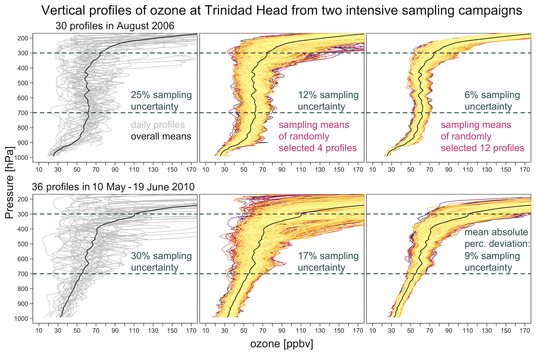
Figure 1 Demonstration of ozone variability from two intensive sampling campaigns (30 profiles in August 2006 and 36 profiles in 10 May–19 June 2010 at Trinidad Head, California) and sampling variability of subsampled means: individual sondes and the overall means are shown in the left panels, and the variabilities of subsampled means are generated in the middle and right panels by randomly selecting 4 or 12 sondes over 1000 times, respectively. This analysis demonstrates that the sampling uncertainty on monthly means in the free troposphere can be reduced by half if the samples are increased from 4 to 12 sondes a month (evaluated by mean absolute percentage deviation at 10 hPa resolution layers).

No similar intensive daily sampling campaigns are available from Hilo, Hawaii (e.g., at most, only 14 profiles were launched in March 2001 during the TRACE-P campaign; Oltmans et al., 2004). However, by comparing the ranges of the 5th and 95th percentiles in the free tropospheric ozonesonde records at Trinidad Head and Hilo, we find similar variability in June–July–August and September–October–November and a modestly higher variability at Hilo in December–January–February and March–April–May (Fig. S1 in the Supplement; the implications for stratospheric intrusions will be discussed later). We can thus expect that the sampling issue is not less important in the tropics than in northern mid-latitudes.

To translate the impact of sampling bias on monthly means into trends, we utilize the monthly mean time series of nighttime temperature and ozone at Mauna Loa Observatory (MLO), which are representative of the lower free troposphere (see Sect. 2 for data descriptions). Figure 2 shows the impact of sampling bias on trend detection, based on monthly means from full sampling (7 d per week) and once-per-week sampling conducted only on Sunday or Tuesday (these two days of the week are chosen to represent the extreme cases; the detailed comparison of the trends from each day of the week will be discussed in Sect. 3, and the complete daily time series are shown in Fig. S2); thus, each month mean is produced from ∼ 30 or ∼ 4 daily values, respectively. We can clearly see how the sampling biases are produced due to reduced sampling. For the temperature data, even though some differences can be observed, the trend and its uncertainty are similar between the results from the full and subsampled records. The bias in the once-per-weekly sampled ozone monthly means can be very large in some cases (e.g., greater than 10 ppbv, also indicated in Fig. 1), indicating that ozone is far more variable than temperature. The MLO ozone trends based on once-per-week sampling can be biased high by 29 % or biased low by −46 % depending on different days of the week. This figure also shows that, even though over 40 years of weekly ozone data were collected, trends can still go undetected when the samples are not representative.

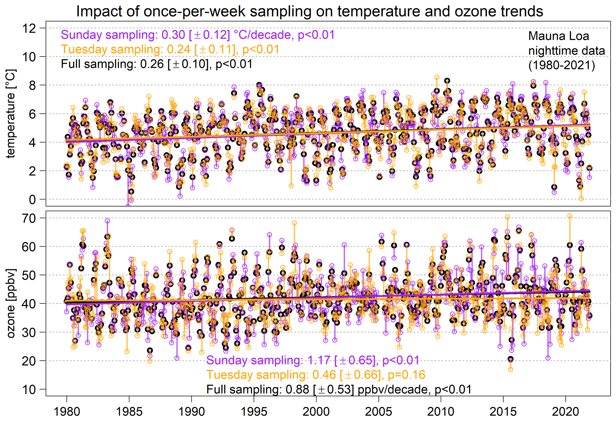
Figure 2 Demonstration of sampling bias from once-per-week sampling in monthly means and trends over 1980–2021 (nighttime temperature and ozone at MLO). Each point represents a monthly mean, aggregated from full sampling (black) or once-per-week sampling conducted only on Sunday (red) or Tuesday (blue). Each vertical range represents the magnitude of sampling bias in a given month. Trends and associated uncertainty estimates are based on the basic model (M1).

Quantitatively, if we compare each ozone daily value to its monthly mean at MLO over 1980–2021, the mean absolute deviation is 20 % or 8 ppbv (in Fig. S1, average deviations of 19 % above Trinidad Head and of 25 % above Hilo are found between individual sondes and their seasonal climatologies in the free troposphere; thus, so the sampling variability is roughly consistent between sonde and surface-based observations). Therefore, the main topic of this study can be stated as follows: how many samples in a month are required to eliminate the impact of a 20 % inter-daily variation on monthly means and trend estimates in an acceptable range? Note that the sampling deviation associated with each daily value represents the true ozone inter-daily variability and should not be considered to be sampling bias; the sampling bias occurs only if we use limited samples to estimate the monthly mean value or trend.

To better quantify the impact of sampling on trend detection, it is important to distinguish between the effect of sample size and sampling bias. Traditionally, the trend analysis of atmospheric composition time series often implicitly assumes that the samples (in this case, monthly mean values) are representative and can be used to assess trends; hence, sample size is the major factor to determine for how long the trends can be detected (assuming that the magnitude of the trend, the data variability, and the autocorrelation are constants; Weatherhead et al., 1998). Therefore, in order to clarify the conceptual difference, we define sample size as the number of points used to fit a statistical model (regardless of the sampling rate), and we define undercoverage bias as a type of sampling error resulting from statistical inference based on sparse or insufficient samples. This conceptual difference can be clearly shown in Fig. 2: the three estimates of ozone trends are based on the same sample size (i.e., the same number of total monthly means), but the trend estimates from reduced samples are severely biased due to undercoverage bias. This work aims to investigate the impact of a series of biased (or non-representative) monthly means on long-term trends.

The goals of this study are as follows: (1) determine the minimum number of ozone observations necessary for accurate trend quantification in the tropical free troposphere, (2) develop optimal sampling strategies that will improve trend detection when faced with limited resources, and (3) leverage co-located observations (e.g., temperature and humidity) and climate indices (e.g., El Niño–Southern Oscillation (ENSO) and quasi-biennial oscillation (QBO)) to improve trend detection through multiple linear regression techniques. Previous attempts to evaluate free tropospheric ozone trends are typically adjusted by ENSO and QBO only (which is the standard approach for stratospheric ozone trends). We aim to show that adjustments based on co-located meteorological observations are more pertinent to tropospheric ozone trend detection and attribution. Section 2 introduces the data sets used in this study and includes a discussion on how the trend and its uncertainty are estimated. Section 3 presents a thorough investigation of the impact of different sampling schemes on the bias in monthly means and trends. Section 4 provides a summary of this study.

2 Data and method

2.1 In situ measurements

In this study, we used the hourly ozone data set measured at Mauna Loa Observatory (MLO), Hawaii (19.5° N, 155.6° W; 3397 m above sea level; Oltmans and Komhyr, 1986; NOAA GML, 2023c) to investigate the impact of different sampling frequencies and strategies on the estimates of monthly means and trends, with a special focus on the quantification of improvements in trend and uncertainty estimates when the sampling frequency is increased. Since MLO is located in the central North Pacific Ocean and at the northern edge of the tropics, ozone variability at MLO is impacted by mid-latitude dry air masses from the north and west and tropical moist air masses from the south and east (Gaudel et al., 2018; Cooper et al., 2020). Lin et al. (2014) found that the relative frequency of dry and moist air mass transport from high latitudes (typically higher ozone) and low latitudes (typically lower ozone) can be influenced by short-term climate variability, such as ENSO and the Pacific Decadal Oscillation. Therefore, an adjustment for meteorological and climate variability is important for quantifying the long term-trend at MLO (Chang et al., 2021).

The MLO record is an ideal test bed for investigating free tropospheric sampling issues because (1) MLO is a high-elevation site, and nighttime ozone at MLO is representative of the lower free troposphere (Price and Pales, 1963; Oltmans and Komhyr, 1986; Tarasick et al., 2019; Cooper et al., 2020), and (2) even though some large interannual variability is present, the overall trends have been roughly linear since the mid-1970s (Chang et al., 2021, 2023a), and, therefore, the results from different sampling tests are comparable (e.g., if the trends are strongly varying between different time periods, it will be difficult to distinguish between the influence of the sampling error and that of nonlinearity in trends). Note that, since daytime data are excluded to avoid the influence of localized anthropogenic emissions (Cooper et al., 2020), no noticeable offsets or heterogeneities between different days of the week, such as the ozone weekend effect, are found in the MLO nighttime ozone record (see Fig. S3).

Once-per-day nighttime ozone averages (08:00–15:59 UTC) at MLO are calculated to represent lower free tropospheric ozone above Hawaii. While reliable hourly ozone observations are available at MLO for the periods 1957–1959 and 1973–1979 (Cooper et al., 2020), colocated meteorological data are more complete from the late 1970s; therefore, our study focuses on the 42-year period from 1980 to 2021. We use a 50 % data coverage criterion to determine the data availability; e.g., we require 15 daily averages in a month. At the daily level, only 757 out of 15 341 (4.9 %) daily ozone values were missing for the 42 years over 1980–2021. At the monthly level, 12 out of 504 (2.4 %) monthly values failed to meet the 50 % data coverage criterion (listed in Table S1 in the Supplement). To avoid selecting non-representative subsamples, data from those 12 months are discarded from our sampling analysis. Links for all of the data sets are provided in the “Code and data availability” section.

The measurement uncertainty for the MLO records (typically ∼ 2 %–4 %) is assumed to be random and is not explicitly taken into account in our analysis (in addition, the daily nighttime averages are expected to smooth out some measurement uncertainty). Nevertheless, if the measurement uncertainty is not random, its effect is likely to be similar to that of the sampling bias, and their total uncertainty is expected to be propagated (and not neutralized).

2.2 Statistical models for evaluating trends and uncertainties

Trend estimates are derived and compared based on the time series produced from the complete data record (full sampling) and reduced subsamples (according to different sampling strategies) in two stages: in the first stage, only fundamental components for time series decomposition are considered for trend detection, i.e., a seasonal cycle and a linear trend; in the second stage, several meteorological variables and climate indices are incorporated into the model in order to improve the trend estimate as adjustments for meteorology and short-term climate variability are often considered to be important for attributing ozone variability (Lin et al., 2014; Porter et al., 2015; Chang et al., 2021). Let y_t, $t=\mathrm{1},\mathrm{\dots },n$ be the ozone mean time series. Each mean value is produced by an aggregation of available data collected over a temporal interval t (typically on a monthly scale). The statistical models for the first and second stages can be expressed as outlined below.

$$\begin{array}{c}{\displaystyle }\text{M1 (basic model):}\\ {\displaystyle }\begin{array}{rl}{\displaystyle }{y}_t=& {\displaystyle }{\mathit{\alpha }}_{\mathrm{0}}+\left[{\mathit{\alpha }}_{\mathrm{1}}\sin \left(\mathrm{2}\mathit{\pi }{\displaystyle \frac{\text{Month}}{\mathrm{12}}}\right)+{\mathit{\alpha }}_{\mathrm{2}}\cos \left(\mathrm{2}\mathit{\pi }{\displaystyle \frac{\text{Month}}{\mathrm{12}}}\right)\right.\\ {\displaystyle }& {\displaystyle }\left.+{\mathit{\alpha }}_{\mathrm{3}}\sin \left(\mathrm{2}\mathit{\pi }{\displaystyle \frac{\text{Month}}{\mathrm{6}}}\right)+{\mathit{\alpha }}_{\mathrm{4}}\cos \left(\mathrm{2}\mathit{\pi }{\displaystyle \frac{\text{Month}}{\mathrm{6}}}\right)\right]\\ {\displaystyle }& {\displaystyle }+{\mathit{\beta }}_{\mathrm{0}}t+N_t.\end{array}\\ {\displaystyle }\text{M2 (full model):}\\ {\displaystyle }\begin{array}{rl}{\displaystyle }{y}_t=& {\displaystyle }{\mathit{\alpha }}_{\mathrm{0}}+\left[{\mathit{\alpha }}_{\mathrm{1}}\sin \left(\mathrm{2}\mathit{\pi }{\displaystyle \frac{\text{Month}}{\mathrm{12}}}\right)+{\mathit{\alpha }}_{\mathrm{2}}\cos \left(\mathrm{2}\mathit{\pi }{\displaystyle \frac{\text{Month}}{\mathrm{12}}}\right)\right.\\ {\displaystyle }& {\displaystyle }\left.+{\mathit{\alpha }}_{\mathrm{3}}\sin \left(\mathrm{2}\mathit{\pi }{\displaystyle \frac{\text{Month}}{\mathrm{6}}}\right)+{\mathit{\alpha }}_{\mathrm{4}}\cos \left(\mathrm{2}\mathit{\pi }{\displaystyle \frac{\text{Month}}{\mathrm{6}}}\right)\right]\\ {\displaystyle }& {\displaystyle }+{\mathit{\beta }}_{\mathrm{0}}t+{\mathit{\beta }}_{\mathrm{1}}\text{WindSpeed}+{\mathit{\beta }}_{\mathrm{2}}\text{WindDirection}\\ {\displaystyle }& {\displaystyle }+{\mathit{\beta }}_{\mathrm{3}}\text{Temperature}+{\mathit{\beta }}_{\mathrm{4}}\text{RelativeHumidity}\\ {\displaystyle }& {\displaystyle }+{\mathit{\beta }}_{\mathrm{5}}\text{Dewpoint}+{\mathit{\beta }}_{\mathrm{6}}\text{ENSO}+{\mathit{\beta }}_{\mathrm{7}}{\text{QBO}}_{\text{30\hspace{0.17em}hPa}}\\ {\displaystyle }& {\displaystyle }+{\mathit{\beta }}_{\mathrm{8}}{\text{QBO}}_{\text{50\hspace{0.17em}hPa}}+N_t.\end{array}\end{array}$$

In the above, α₀ is the intercept; $\mathit{\{}{\mathit{\alpha }}_k,k=\mathrm{1},\mathrm{\dots },\mathrm{4}\mathit{\}}$ is a set of coefficients jointly representing the seasonal cycle; β₀ is the trend value; $\mathit{\{}{\mathit{\beta }}_k,k=\mathrm{1},\mathrm{\dots },\mathrm{8}\mathit{\}}$ is a set of coefficients associated with different meteorological variables and climate indices, respectively; and N_t is the residual series. Note that the M2 (full model) does not represent our final trend model as a variable selection procedure will be carried out to determine which variables are the most statistically and scientifically meaningful.

The models are fitted based on the least squares (LSs) and least absolute deviations (LADs) for the estimations of mean and median trends (as well as other coefficients; albeit, the focus is placed on the trend estimate), respectively. The estimations of LADs are implemented using quantile regression available from the R package quantreg (Koenker and Hallock, 2001). In addition, the moving block bootstrap (MBB) algorithm is integrated into LS and LAD estimations in order to produce consistent uncertainty estimates between the mean and median trends (Fitzenberger, 1998; Lahiri, 2003). Because the autocorrelation and heteroscedasticity are not invariant between different subsampled time series, an MBB approach is expected to accommodate a larger class of autocorrelation structures and to be more flexible than a fixed autoregressive model, such as an AR(1) or AR(2) process.

The fitting procedure for LS and LAD trends is conducted iteratively and is outlined as follows: (1) for each iteration, a trend model is fitted to randomly selected multi-blocks of resampled data, and the corresponding bootstrapped trend value is extracted, and (2) the final trend estimate (and its 1σ uncertainty) is produced by the mean (and standard deviation or SD) of the bootstrapped trends from 1000 iterations. The code for implementing median regression based on the MBB algorithm is documented in the Tropospheric Ozone Assessment Report (TOAR) statistical guidelines (Chang et al., 2023b).

In terms of fitting quality, root-mean-square (percentage) deviation and mean absolute (percentage) deviation are used to assess the overall predictive performance:

$$\begin{array}{c}{\displaystyle }\text{RMSD}={\left({\displaystyle \frac{{\sum }_{t=\mathrm{1}}^n({\widehat{y}}_t-y_t{)}^{\mathrm{2}}}{n}}\right)}^{\mathrm{1}/\mathrm{2}},\text{ and }\\ {\displaystyle }\text{MAD}={\displaystyle \frac{{\sum }_{t=\mathrm{1}}^n|{\widehat{y}}_t-y_t|}{n}}\text{for the units of ppbv};\\ {\displaystyle }\text{RMSPD}={\left({\displaystyle \frac{{\sum }_{t=\mathrm{1}}^n\left(\right({\widehat{y}}_t-y_t)/y_t{)}^{\mathrm{2}}}{n}}\right)}^{\mathrm{1}/\mathrm{2}},\text{ and }\\ {\displaystyle }\text{MAPD}={\displaystyle \frac{{\sum }_{t=\mathrm{1}}^n\left|\right({\widehat{y}}_t-y_t)/y_t|}{n}}\text{for the units of percentage}.\end{array}$$

In the above, ${\widehat{y}}_t$ is the fitted value of y_t. To explicitly quantify the sampling impact, by using the same methodology, we can define the undercoverage bias as $(s_{\mathrm{r}}-s_{\mathrm{c}})/s_{\mathrm{c}}$, where s_c is the statistic of interest (e.g., can be either the monthly mean, trend value, or trend uncertainty) derived from the complete data set, and s_r is the statistic derived from the reduced or subsampled data set; thus, RMSPD (root-mean-square predictive difference) and MAPD (mean absolute percentage deviation) can also be used to assess the improvement due to sampling enhancement.

It should be noted that Chang et al. (2021) used an adaptive nonlinear trend technique (i.e., regression splines fitted through generalized additive models (GAMs); no assumptions regarding the shape of trends is required in advance) to model the ozone variability at MLO and found that the nonlinearity captured by the GAM is largely diminished and becomes roughly linear after the meteorological variability is accounted for, indicating that the nonlinearity in the ozone time series at MLO can be attributed to meteorological influence. Therefore, a change point analysis of long-term trends at MLO is not considered in this study.

3 Results

3.1 Quantifying undercoverage bias in monthly means and trends from weekly samples

Figure 3 shows the scatterplots between the monthly means based on all available (complete) daily nighttime observations and monthly means aggregated from (reduced) weekly samples, according to each day of the week and different bias exceedance thresholds (e.g., the dark-red color indicates that the absolute sampling bias of the mean from reduced samples is greater than 25 % of the mean from complete samples in a given month). In contrast to RMSD and MAD, which represent the overall predictive performance, bias exceedance rate is a measure focusing on the frequency of extreme sampling bias. Overall, even though we do not observe strong systematic biases from the scatterplots (as indicated by the correlation line in blue), some large discrepancies are present (see Table 1 for the results by each day of the week). On average, 13.5 % and 5.1 % of the months show the bias exceedance rate to be greater than 15 % and 20 % of the monthly means, respectively. Depending on the locations of these discrepancies in the time series, they can obscure the true trend estimate, as shown in Fig. 2.

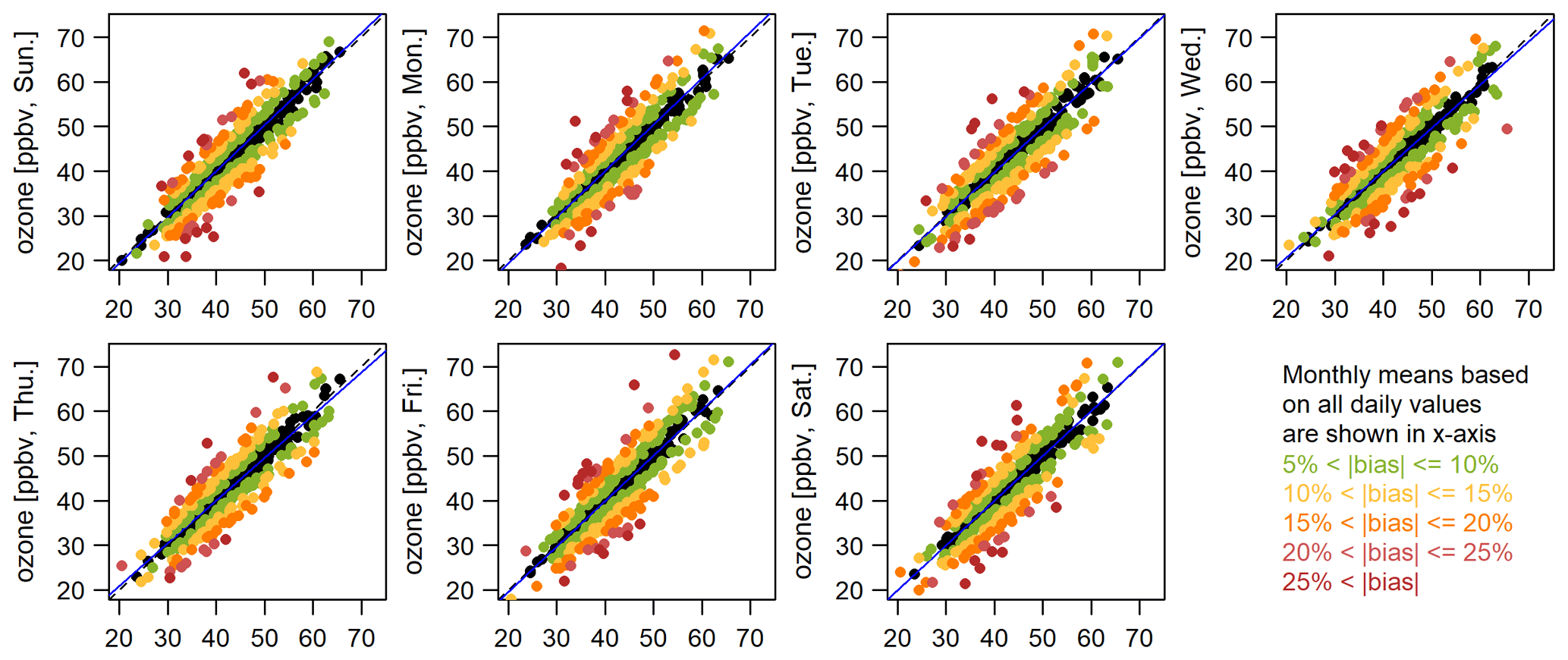
Figure 3 Demonstration of exceedance bias (at different thresholds) from once-per-week samples in monthly means: panels show the scatterplots between monthly means based on full sampling (x axis) and once-per-week sampling (y axis, by each day of the week). The result are based on daily nighttime observations measured at MLO (1980–2021). The solid blue line in each panel is the 1:1 line, and the dashed blue line represents the overall correlation.

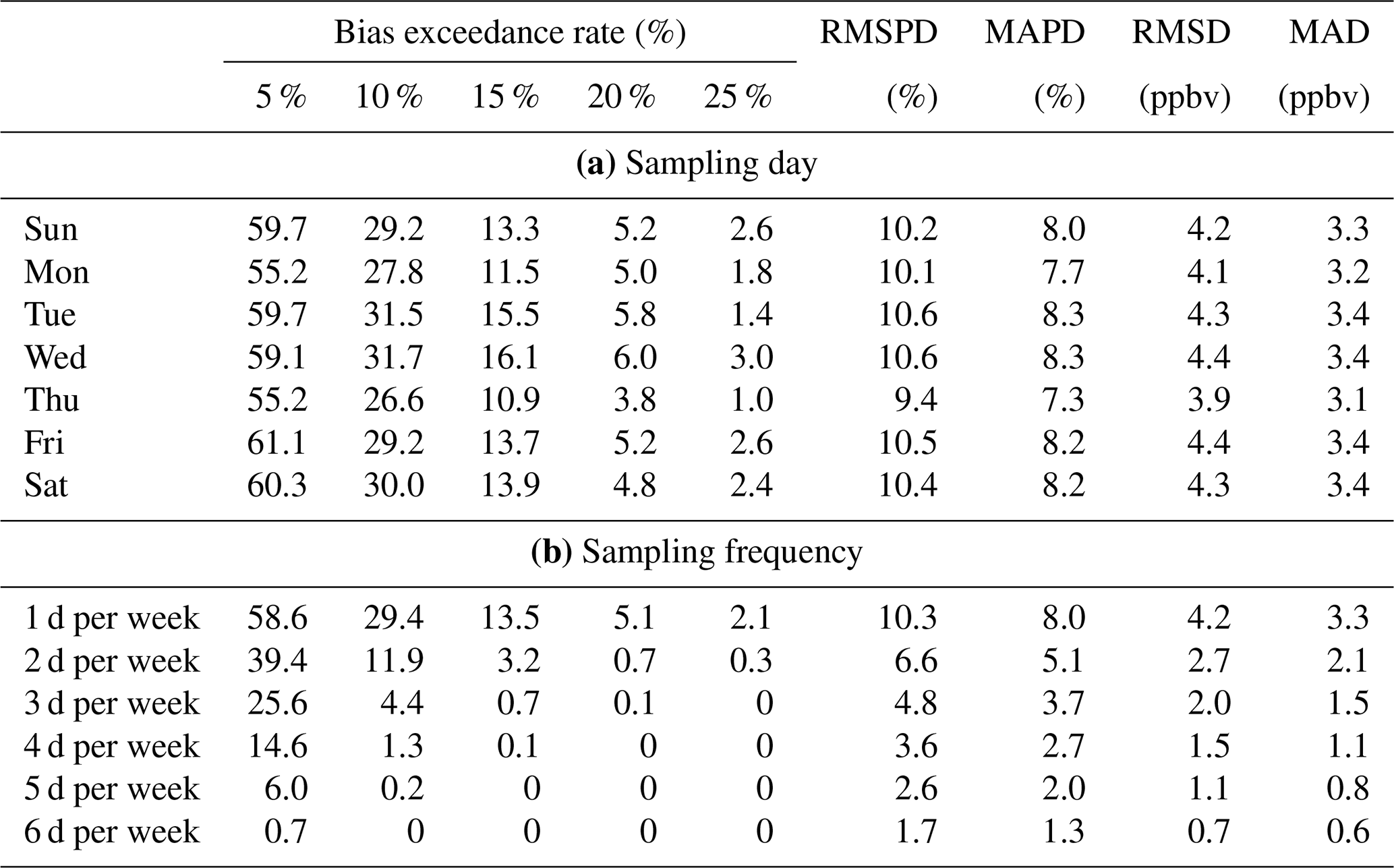
Table 1 Undercoverage bias in monthly means (1980–2021) based on (a) once-per-week sampling by each day of the week and (b) different sampling frequencies per week (average over all possible subsets). Bias exceedance rate indicates the frequency at which the absolute sampling bias of the mean from reduced samples is greater than a threshold (5 %–25 %) of the mean from complete samples.

A once-per-week sampling analysis is carried out by estimating the mean and median trends based on each day of the week and different time periods. The following discussion is based on Fig. 4a and c:

• First of all, it is important to separate the effect of sample size (for fitting the trend model) from that of undercoverage bias (due to sparse sampling). The scenario on the left of Fig. 4a indicates the mean trends and 2σ intervals estimated from full sampling (seven samples per week). Trend values are around 0.9 ppbv per decade from 1980, 1990, and 2000, but the uncertainty grows when the time periods become shorter. This implies that high certainty (2σ confidence level) in trends cannot be attainable over 2000–2021 and 1995–2021, mainly because the time series are too short (i.e., roughly 30 years of continuous data are required to detect the signal at this magnitude, given the fact that the trends are relatively linear over 1980–2021).

• However, given the fact that the sample size for trend estimation is the same (i.e., the total number of monthly means for full and weekly sampling), if we sample on Tuesday or Wednesday only, high certainty in mean trends cannot be obtained even with 30 years of data (1990–2021); and if we sample on Tuesday only, high certainty in mean trends cannot be obtained even with 40 years of data (1980–2021). In these cases, we conclude that the sampling biases from weekly samples are not neutralized even when very long-term records are considered, and the undercoverage biases persistently reduce trend accuracy.

• So far, the above discussion is based on the mean estimator. The big picture remains similar if we compare the results between the mean and median estimators. Comparable patterns can be observed when the time series is sufficiently long (> 30 years), and it is not unexpected to see some noticeable discrepancy when the sample size is low (also confounding with sampling bias in weekly samples). Note that the discrepancy between mean and median trend estimates can be mainly attributed to ozone heterogenous variability (Chang et al., 2023a), while the discrepancy between trend uncertainties can also be attributed to different optimized algorithms (if the regression assumptions are not severely violated, the LS method tends to produce a narrower uncertainty than other algorithms; see Fig. S4 for a further demonstration).

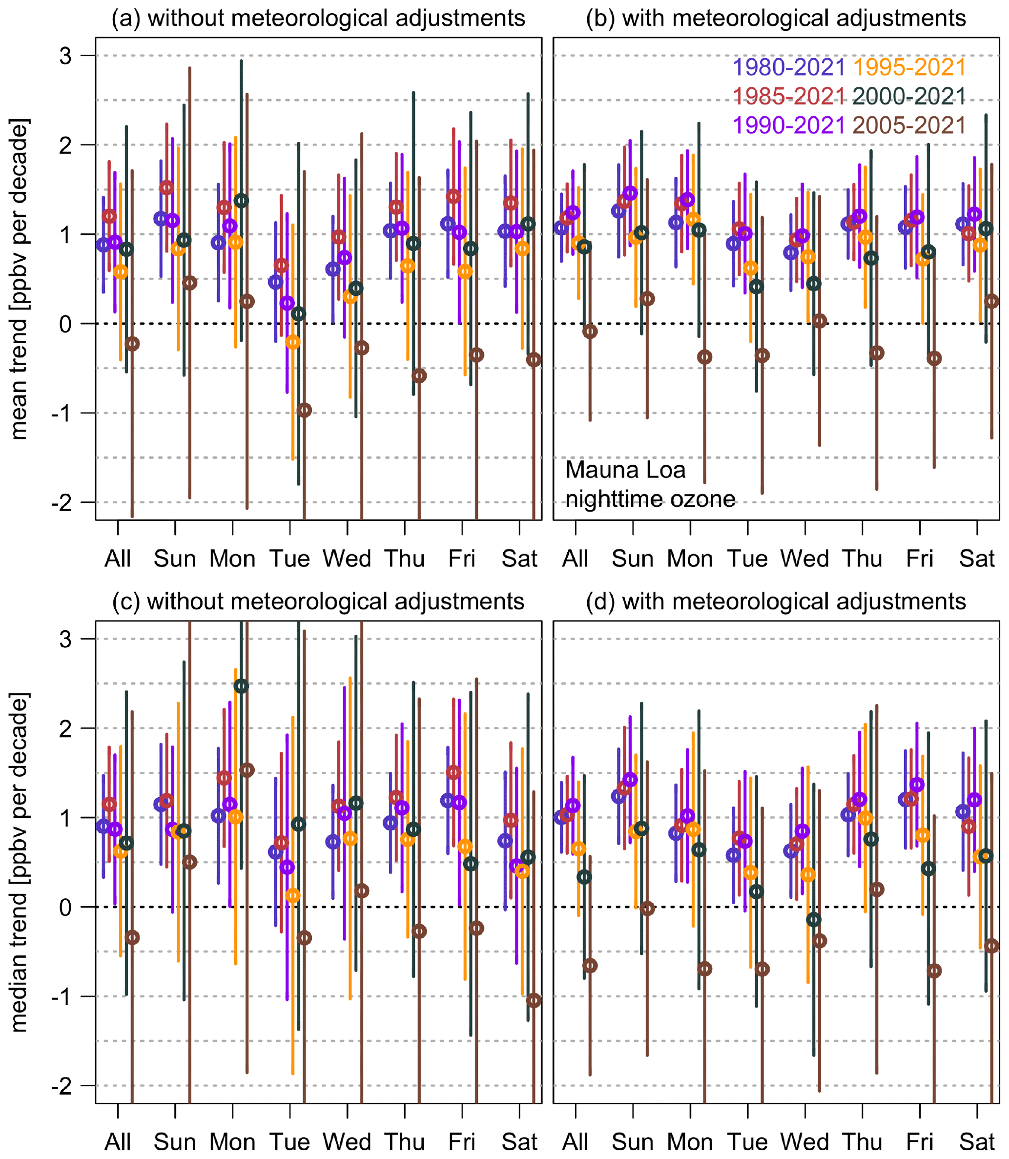
Figure 4 MLO ozone trends and 2σ intervals derived from the mean (a, b) and median (c, d) estimators, without (a, c) and with (b, d) meteorological adjustments, respectively. In each panel, the results are based on monthly means aggregated from full sampling (labeled as “all”) and once-per-week sampling (labeled by day of the week) for six different time periods.

3.2 Strategies for improving trend detection: attribution of data variability

To further investigate the cause of sampling bias and to improve the trend estimate, for the next step, we aim to attribute the data variability by incorporating meteorological variables and climate indices. Since meteorological variables are often correlated, we need to evaluate which variables have the best predictive performance and determine a simple yet powerful model that accounts for the most variability.

The variable selection process is described in Appendix A. In the following analysis, we use dew point and ENSO (in addition to the basic model M1) as the most effective covariates in our best trend model for the MLO ozone record. To differentiate from the basic model, we refer to the trend estimate from the best model as the meteorologically adjusted trend (since dew point is the main attributor). We then applied the best trend model to the once-per-week sampling test (see Fig. 4b and d). Through meteorological adjustments, this uncertainty attribution approach improves the precision of the ozone trends at all timescales, and the uncertainty is reduced by 35 % on average (SD=7 %) when focusing on full sampling. This approach also improves the accuracy of the trends which are based on once-per-week sampling; in particular, it leads to great improvement in the trend bias from Tuesday sampling. These findings suggest that the sampling bias in trends can be substantially reduced through a consideration of colocated meteorological variability.

3.3 Quantifying the benefit of increasing sampling frequency

This section extends the current scope beyond once-per-week sampling. The purpose is to investigate the strengths of different sampling schemes and, eventually, to develop the best approach to reduce sampling bias with a minimal cost (i.e., fewer additional samples). However, before this analysis is carried out, it is desirable to fully understand the relationship between the enhancement in sampling rate and the reduction in sampling bias.

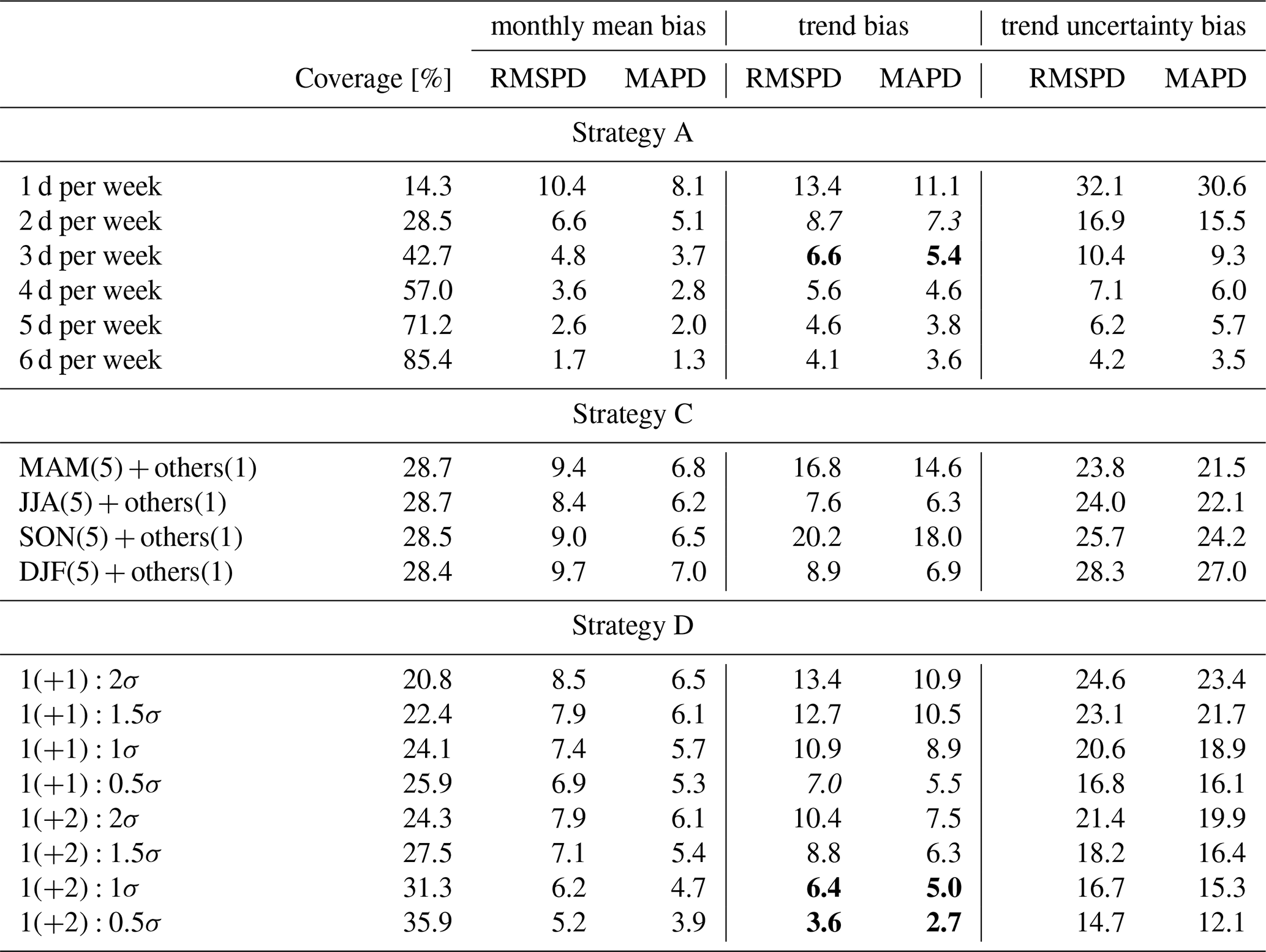
We summarize the sampling strategies adopted in this study in Table 2. The most straightforward extension is to simply increase the sampling days per week (strategy A). The improvement in the sampling bias in monthly means is provided in the second part of Table 1. For the interpretation, (1) the 10 % bias exceedance rate in monthly means is reduced from 29.4 % to 11.9 % if we increase the sampling frequency from once per week to twice per week; (2) when focusing on the extreme cases, monthly mean bias exceedance above 25 %, 20 %, 15 %, and 10 % can be eliminated based on schemes of three to six samples per week, respectively; and (3) three samples per week seems feasible in terms of limiting the 10 % bias exceedance rate within 5 % and limiting the average RMSPD and MAPD within 5 % (or below 2 ppbv). In terms of sampling bias in trends for strategy A, Fig. 5 shows the mean trend and 2σ uncertainty for some cases based on one to three samples per week (another visualization is provided in Fig. S9 by showing the full-sampling variations for the periods 1990–2021 and 2000–2021; e.g., twice per week might also occur on Monday and Thursday, Monday and Friday, etc). From a sampling frequency of at least 3 d per week (or 43 % data coverage), the trend estimate from each individual scenario is fairly close to the true trend (from full sampling), whereas, quantitatively, five samples per week are required to reduce the overall RMSPD and MAPD trend biases to 5 % (see the first part of Table 3 and the later discussion).

Table 2 Sampling strategies adopted in this study.

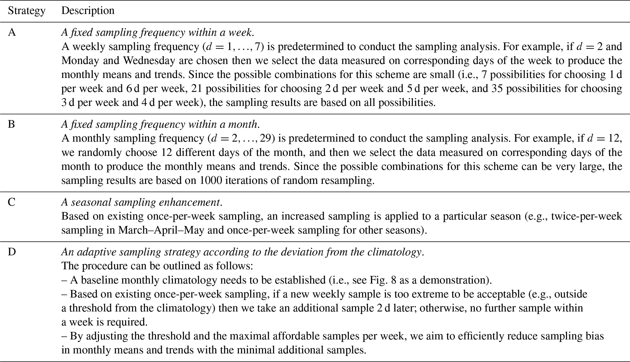
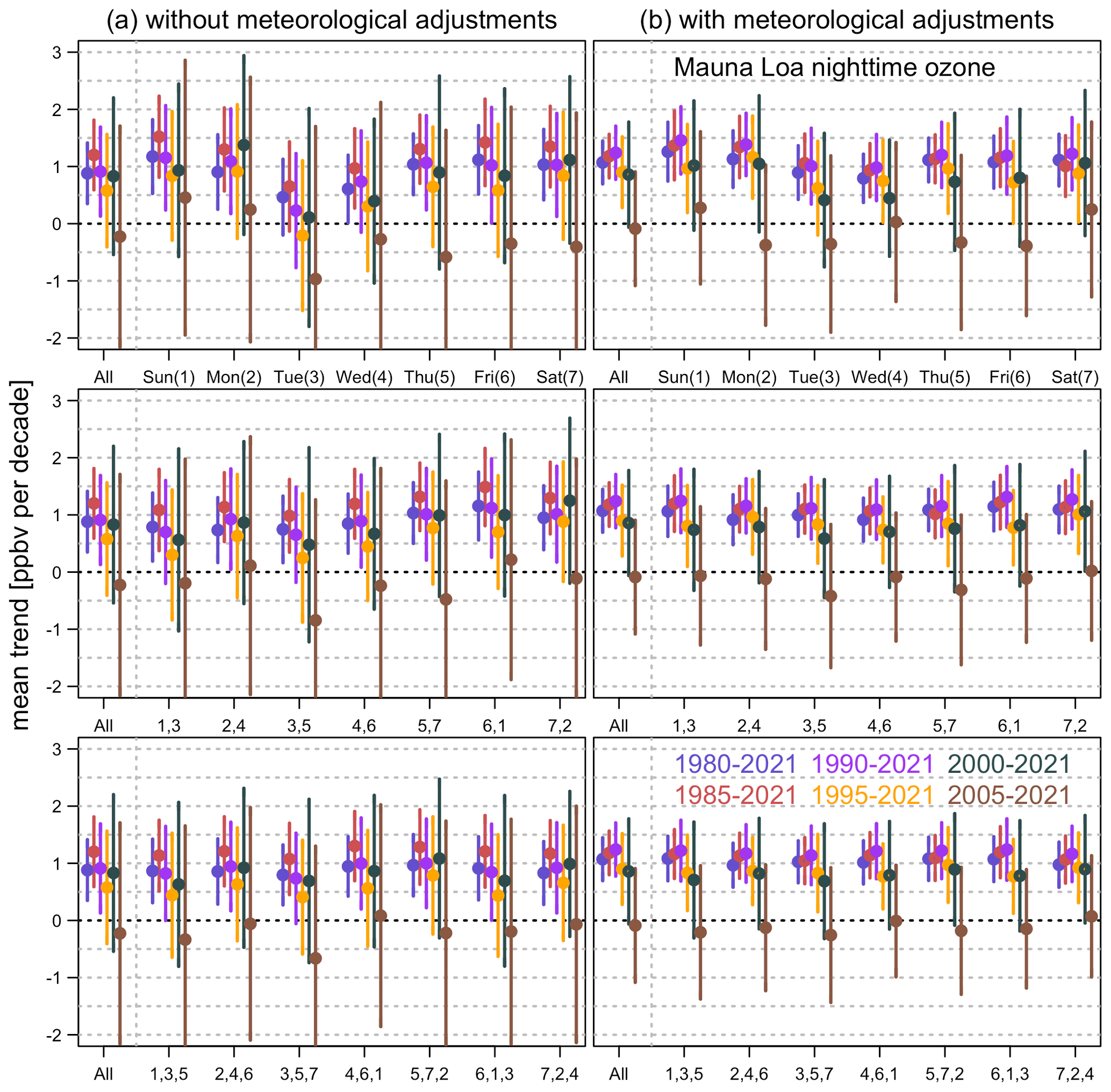
Figure 5 Same as Fig. 4 but based on the mean estimators only and (from top to bottom) one to three samples per week (e.g., the label “1,3,5” indicates sampling on Sunday, Tuesday, and Thursday).

Table 3 Undercoverage bias in monthly means, trend estimate, and trend uncertainty from different sampling strategies (1990–2021, with meteorological adjustments). Strategy A is based on different sampling days per week for all months. Strategy C is based on once-per-week sampling for all months, incorporated with additional sampling of 4 d per week in a specific season (so the data coverage is similar to sampling of 2 d per week for all months). Strategy D is an anomaly-based strategy: $X(+Y):Z\mathit{\sigma }$ denote a sampling scheme based on X regular samples per week with, at most, Y extra samples per week according to the Zσ tolerance range. Particular cases (shown in italic font for 2 d per week and $\mathrm{1}(+\mathrm{1}):\mathrm{0.5}\mathit{\sigma }$ or in bold font for 3 d per week, $\mathrm{1}(+\mathrm{2}):\mathrm{1}\mathit{\sigma }$, and $\mathrm{1}(+\mathrm{2}):\mathrm{0.5}\mathit{\sigma }$) indicate that fewer samples are used to achieve a better estimation by Strategy D.

Since the sampling frequency is the only control variable in the following analysis, hereafter, unless additional demonstrations are needed to highlight the influence of other factors, we place the focus on the meteorologically adjusted mean trends over 1990–2021. To further demonstrate the challenges with a low sampling rate, we aim to quantify the improvement in sampling bias by increasing the number of samples per month (strategy B in Table 2). We evaluate the sampling bias at two stages. The first stage is to investigate the statistical power at different sampling frequencies (the likelihood of detecting a trend from subsamples based on the fact that a true trend is observed in the full MLO record). In the second stage, we define the acceptable rate according to how many random samples produce a trend that falls within ± 10 % of the truth (after excluding the samples which fail to detect the signal in the first stage). With this approach, we are able to explicitly quantify the percentages of samples that can (1) detect the signal and (2) produce an accurate estimate.

Figure 6 shows the full ranges of individual sampling bias and variability for 2, 4, 8, 12, 16, and 20 samples per month, along with the resulting statistical power and acceptable rate. A dogmatic approach to comparing trends is based on the intersection of uncertainty ranges; two trends are deemed to have no “significant difference” if their confidence intervals overlap. Figure 6 clearly highlights that this dichotomy is simply unsatisfactory: despite the subsampled uncertainty estimates intersecting with the true range, there is no justification for one to conclude that there is no sampling difference between the results for 4 and 12 samples per month. For 12 samples per month, 69.7 % of the samples yielded a trend with a 2σ interval greater than zero. The acceptable rate indicates that 53.3 % of the samples were able to detect the trend within ± 10 % of the true value. In contrast, a strategy of four samples per month yielded a low statistical power of 40.1 %, and only 9.7 % of the samples could detect the trend accurately. A strategy of just two samples per month yielded an acceptable rate of zero because the subsamples either severely overestimated the trend or were not able to detect the trend.

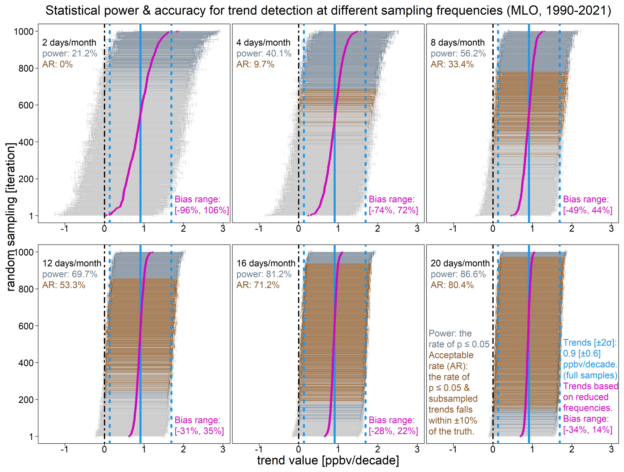
Figure 6 Statistical power and accuracy for trend detection: this figure illustrates how trend values can become noisy and uncertain when the data set is thinned from full sampling (every day of the month) to 2, 4, 8, 12, 16, and 20 samples per month. The vertical blue lines represent the 1990–2021 ozone trend based on the full record (without meteorological adjustments), with the solid line being the mean trend value and the dashed lines representing the 2σ interval. For each panel, subsamples are generated randomly and independently over 1000 iterations, and resulting subsampled trends are sorted along the y axis from the lowest to the highest values (purple line – the lowest and highest values are indicated in the bias range); each horizontal line indicates the 2σ interval. Subsampled trends with p values ≤0.05 (dark gray and orange) are summarized by statistical power. Subsampled trends with p values ≤0.05 and within ± 10 % bias (orange) are summarized by the acceptable rate.

It should be noted that statistical power is heavily affected by the absolute magnitude of the trend and sigma values; thus, we also considered other scenarios. Figure S10 shows the following: (a) when a stronger signal and a lower sigma are present (e.g., signal-to-noise ratio (SNR) >5), a high statistical power (99.9 %) can be achieved at a lower sampling rate, and (b) when a similar signal is present, a lower sigma uncertainty can also enhance the statistical power (from 40.1 % to 73.2 %). Nevertheless, the acceptable rate is still far from ideal for low sampling rates, even if the trend and SNR are strong. A further detailed analysis of strategy B is provided in the Supplement (beyond the selected frequencies in Fig. 6). Overall, based on an extensive evaluation, we conclude that a minimal sampling rate of either 3 regular samples per week (strategy A) or 12 random samples per month (strategy B) is required for the trend statistics to be robust against the sampling impact.

3.4 Cost–benefit strategies for effectively increasing sampling rate

For the situation where three regular samples per week or higher are too expensive to maintain for a given ozonesonde station, we aim to develop a simple cost–benefit strategy to improve upon the existing once-per-week sampling scheme by efficiently reducing sampling bias in monthly means and trends with the minimal cost. Two strategies are proposed in order to achieve this goal (see Table 2). Strategy C is designed for increasing additional samples during a predetermined season (e.g., ozone is typically more variable and less predictable during seasons with frequent stratosphere–troposphere exchange events). Strategy D adopts an anomaly detection approach to temporarily increase the sampling rate based on the sampling deviation against the climatology. The rationale is to first develop a baseline climatology (i.e., monthly mean and SD over 1980–1989). Then, for the period 1990–2021, if any new weekly sample (the first in a week) is too extreme compared to the climatology (e.g., outside monthly mean ± 2 SD), we take a second sample 2 d after the initial sampling date (a third sample can be taken 2 d after the second sampling date if necessary); otherwise, no extra sample within a week is required.

Strategy C is a mixed-sampling approach in which we use once-per-week sampling for all months as the baseline, and then, during a particular season, the frequency is increased to two to seven samples per week (while the other seasons maintain once-per-week sampling) so we can investigate if the overall trend estimate can be improved by (partially or completely) removing specific seasonal sampling biases. In Fig. 7, we show the seasonal trends and biases over 1990–2021 (difference between subsampled trend and the true trend, with meteorological adjustments). This is unexpected in that no consistent improvement in trend precision and accuracy can be seen from extra seasonal samples. Even if we increase the seasonal samples up to full sampling, improvement can only be achieved in June–July–August (JJA) and December–January–February (DJF), while March–April–May (MAM) and September–October–November (SON) still show a strong bias (and are no better than with once-per-week sampling). Table 3 shows the percentage bias from strategies A and C (five samples per week for a particular season and once per week for other seasons so that the coverage rate is similar to twice-per-week sampling for all months); from this table, we can see that, even though monthly mean bias is reduced with strategy C (compared to once-per-week sampling), trend bias is unexpectedly increased in MAM and SON.

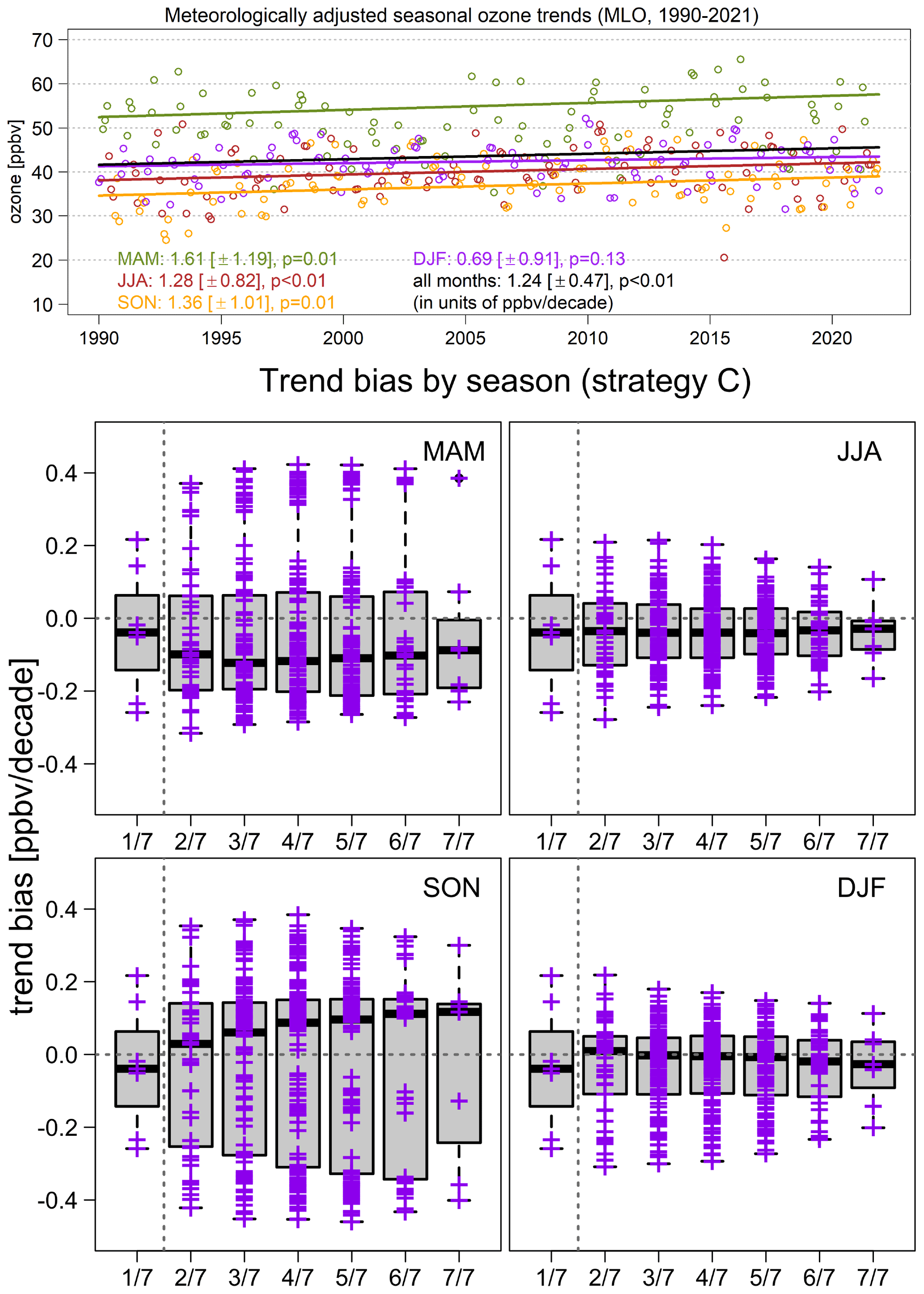
Figure 7 MLO ozone seasonal trends under full sampling (upper panel) and seasonal trend bias (each cross represents the difference between a subsampled trend and the true trend, with meteorological adjustments – lower panel) under mixed sampling (1990–2021, strategy C): $\mathrm{1}/\mathrm{7}$ indicates the baseline scenario representing once-per-week sampling for all months, and $k/\mathrm{7}$ ($k=\mathrm{2},\mathrm{\dots },\mathrm{7}$) indicates x samples per week for a particular season, while the other seasons remain at once-per-week sampling.

The most likely reason for the trend bias in MAM and SON is that these two seasons represent the MLO ozone peak and trough of a year; thus, if we only enhance the sampling in either season, the seasonal variability tends to outweigh the trends (analogously to only sampling the tail of a histogram). In contrast, seasonal variability in JJA and DJF is more consistent with the overall mean; thus, the trend estimates are more likely to be improved (see Figs. S13–S15). The cause of such phenomena can be associated with a well-known sampling fallacy, also known as selection bias (Bateson and Schwartz, 2001) or preferential sampling (Diggle et al., 2010). This fallacy typically occurs when the samples are heavily biased toward a specific subset of the target population. Since there is no guarantee regarding the improvement in trend bias, strategy C is not an ideal sampling approach.

Although we found no direct causality between a reduction in monthly mean bias and trend bias, it is natural to suspect that the extreme sampling biases attached to certain months might be the main attributor to trend bias. Strategy D is an adaptive approach designed for the elimination of sampling bias that is too great to be reasonable or acceptable. As discussed above, we use 1980–1989 ozone data to develop a baseline climatology (i.e., seasonal cycle and SD) and 1990–2021 data to validate the result. Given the fact that the seasonal cycle is accounted for, a tolerance range needs to be defined to determine if the magnitude of the de-seasonalized anomaly is reasonable. The narrower the tolerance range (the higher the sampling rate), the greater the reduction in the extreme sampling bias (see Fig. S16). With this strategy, if we assume, at most, three samples per week, our aim is to find an optimal tolerance range, such that the trend bias is better than the scheme of three regular samples per week (indicating that fewer samples are used to achieve a better estimation). Since the climatological mean and SD vary in different months, the sampling rate is not uniformly distributed across the year. Figure 8 displays the climatology and average monthly sample size based on different tolerance ranges and, at most, three samples per week. We can see that the necessary monthly samples are clearly associated with the monthly variability: the higher the monthly SD (e.g., April), the fewer additional samples are required. Our specification for tolerance is purely based on ozone monthly variability; alternative approaches might be possible if the extreme sampling bias can be attributed to other factors (e.g., extreme weather conditions), but this is beyond the scope of this study.

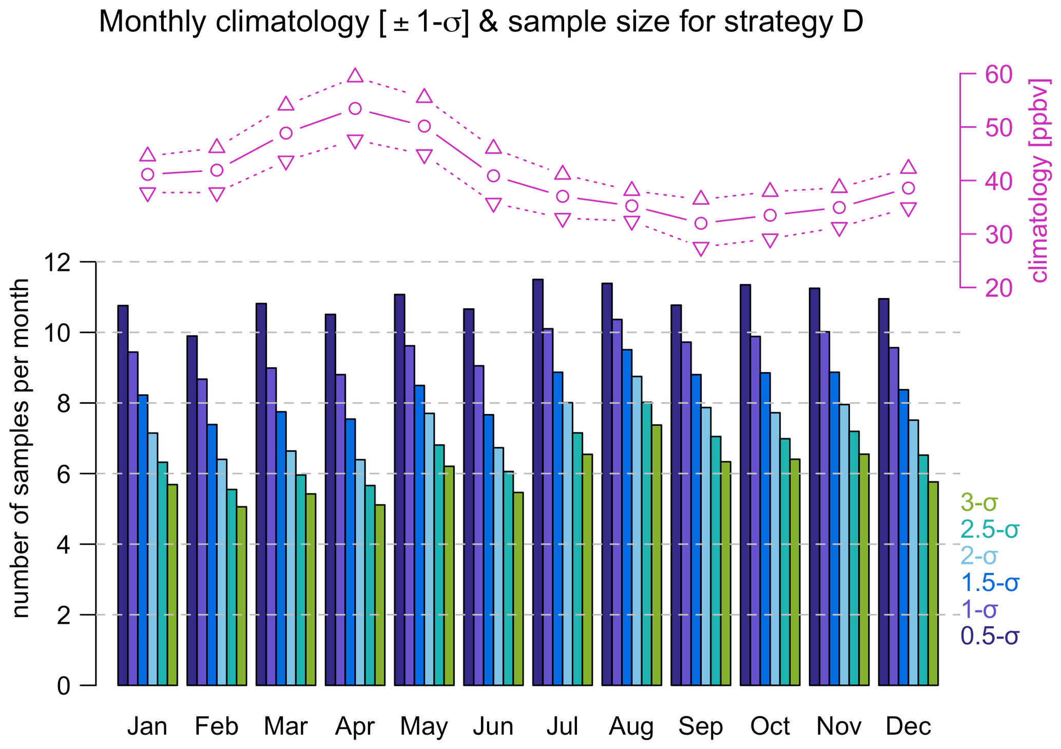
Figure 8 Monthly climatology (± 1 SD) and average samples per month based on, at most, three samples per week and different tolerance ranges (strategy D).

To facilitate a discussion of strategy D, let $X(+Y):Z\mathit{\sigma }$ denote a sampling scheme based on X regular samples per week with, at most, Y extra samples per week according to the Zσ tolerance range (a demonstration is made using the $\mathrm{1}(+\mathrm{2}):\mathrm{2.5}\mathit{\sigma }$ scheme in Fig. 9). The percentage bias and coverage rate for strategy D are summarized in the third part of Table 3:

• When focusing on, at most, two samples per week, the trend accuracy based on the 0.5σ tolerance (∼ $\mathrm{1.8}/\mathrm{7}$) is comparable to $\mathrm{2}/\mathrm{7}$ regular sampling.

• When focusing on, at most, three samples per week, the trend accuracy based on the 1σ tolerance (∼ $\mathrm{2.2}/\mathrm{7}$) is comparable to $\mathrm{3}/\mathrm{7}$ regular sampling. The trend bias can be further reduced to below 5 % if a narrower 0.5σ tolerance (∼ $\mathrm{2.5}/\mathrm{7}$) is applied ($\mathrm{5}/\mathrm{7}$ regular sampling is required to meet the same goal).

Under these circumstances, an improved trend accuracy is achieved with fewer samples than regular sampling, but the bias metrics for monthly means and trend uncertainty remain at similar levels as regular $\mathrm{2}/\mathrm{7}$ or $\mathrm{3}/\mathrm{7}$ sampling; this result indicates that strategy D is only designed for improving trend accuracy. Note that, from the above result, a more constrained tolerance is required to achieve our goal, but a gradual improvement can still be provided by the 2σ or 1.5σ tolerance. This suggests that the adaptive sampling strategy can be tailored to a specific sampling rate according to the budget (by modifying the tolerance range and the maximal samples allowed in a week; see next section).

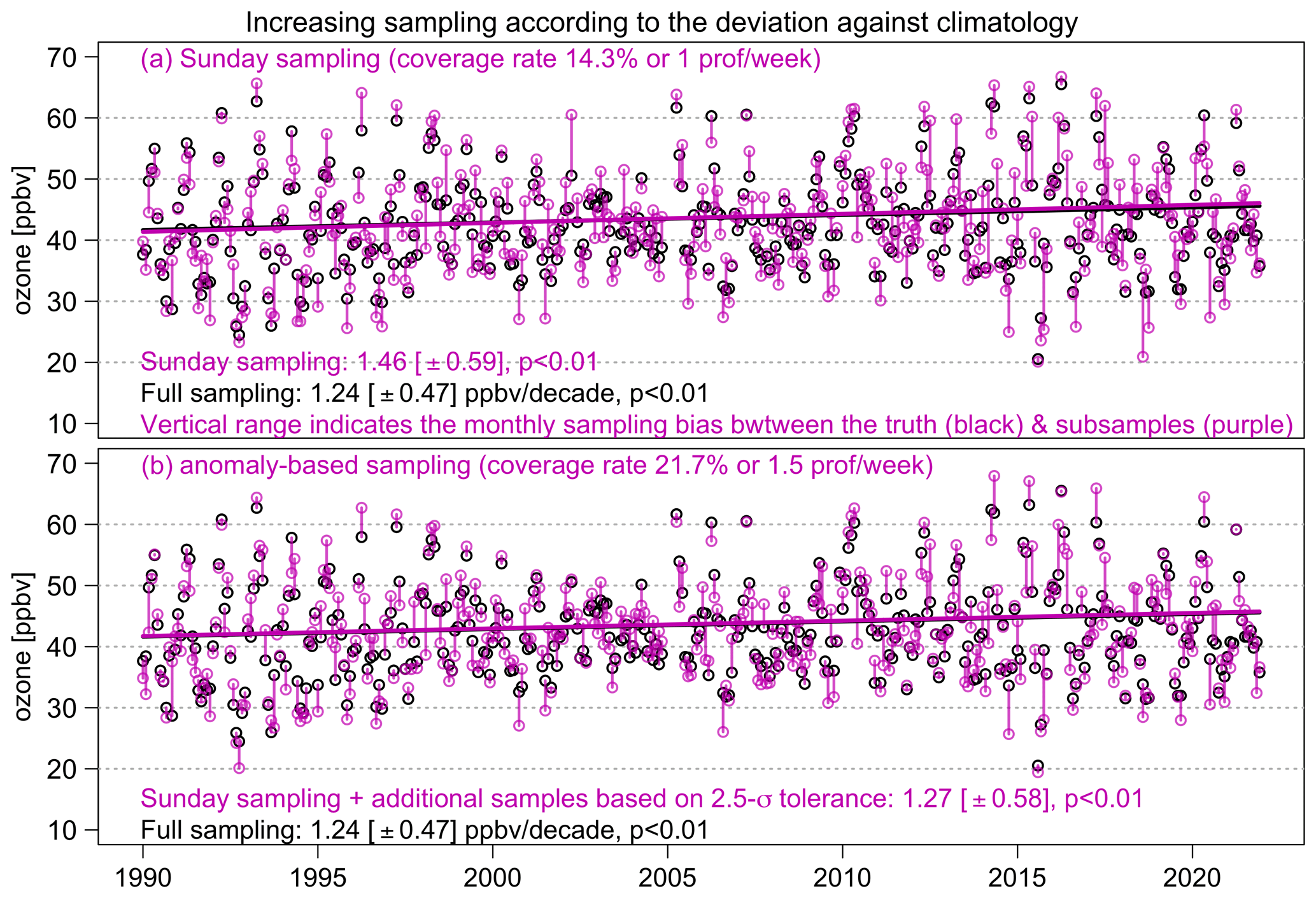
Figure 9 Demonstration of anomaly-based sampling for ozone time series. Panel (a) shows the magnitude of monthly sampling bias between full sampling (black) and once-per-week sampling on Sunday (purple). Panel (b) is based on the same scheme, but additional samples are taken when any weekly samples are found to be outside the 2.5σ range from the climatology (at most, three samples per week). Trends and associated uncertainty estimates are meteorologically adjusted.

3.5 Recommendations on efficient sampling for trend detection

We recognize that, in reality, once-per-week sampling does not imply that the sample is always measured on the same day of the week. We use the ozonesondes launched at Hilo, Hawaii, as an example (19.72° N, 155.05° W; Hilo is ∼ 56 km northeast of MLO with a roughly once-per-week sampling frequency in 1982–2021). The effect of (real) sparse sampling is shown by matching the Hilo ozonesonde launch dates and the MLO surface ozone record (the Hilo data are selected for the same pressure level as MLO), and then the MLO ozone trends are estimated based on the Hilo ozonesonde sampling dates and also by shifting 1, 2, …, 6 d after the colocated dates (Fig. S17). The result shows that a strong sampling bias in trends can be observed from the Hilo ozonesonde sampling scheme and also based on our previous finding that similar amounts of sampling variability can be observed between the Hilo ozonesonde and MLO nighttime ozone records (Fig. S18); therefore, the implications for undercoverage bias from previous discussions are still valid.

We revisit the analysis in Fig. 5 by incorporating the anomaly-based sampling strategy. Figure 10 shows the trends based on the $\mathrm{1}(+\mathrm{1}):\mathrm{0.5}\mathit{\sigma }$, $\mathrm{1}(+\mathrm{1}):\mathrm{1}\mathit{\sigma }$, and $\mathrm{1}(+\mathrm{2}):\mathrm{1}\mathit{\sigma }$ schemes. This demonstrates how we can tailor our sampling scheme to a specific budget by adjusting the tolerance range and the maximal samples per week. These selections are made because previous comparisons (based on 1990–2021) found that the trend accuracy is comparable between two regular samples per week and the $\mathrm{1}(+\mathrm{1}):\mathrm{0.5}\mathit{\sigma }$ scheme and between three regular samples per week and $\mathrm{1}(+\mathrm{2}):\mathrm{1}\mathit{\sigma }$ scheme. Thus, we might be able to reduce the cost without compromising the trend accuracy by omitting some samples which are expected to convey less new information.

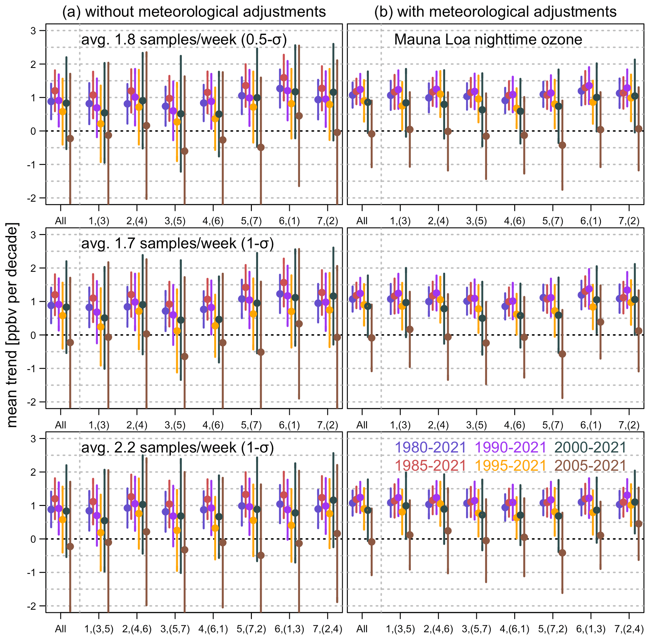
Figure 10 Same as Fig. 5, but the anomaly-based sampling strategy is incorporated. From top to bottom: the $\mathrm{1}(+\mathrm{1}):\mathrm{0.5}\mathit{\sigma }$, $\mathrm{1}(+\mathrm{1}):\mathrm{1}\mathit{\sigma }$, and $\mathrm{1}(+\mathrm{2}):\mathrm{1}\mathit{\sigma }$ schemes. Numbers in parentheses in the x axis indicate the extra sampling days of the week.

In summary, to achieve efficient sampling enhancement for trend detection based upon current once-per-week sampling, we can adjust our adaptive sampling strategy according to the funds available to purchase additional ozonesondes. In terms of annual samples and budget (the cost to launch one ozonesonde is roughly USD 1500 to cover both equipment and personnel costs), we can make the best use of an extra 26 profiles in a year (∼ 1.5 per week) by applying the $\mathrm{1}(+\mathrm{1}):\mathrm{2}\mathit{\sigma }$ scheme. If an additional 42 profiles per year (∼ 1.8 per week) are allowed, we can achieve a similar trend accuracy compared to two regular samples per week by applying the $\mathrm{1}(+\mathrm{1}):\mathrm{0.5}\mathit{\sigma }$ scheme. Likewise, an additional 63 profiles (∼ 2.2 per week) would allow us to produce a trend accuracy comparable to three regular samples per week (the $\mathrm{1}(+\mathrm{2}):\mathrm{1}\mathit{\sigma }$ scheme) (3 profiles per week is equal to 156 profiles per year). Therefore, our ultimate goal can be achieved without fully sampling 3 d per week (and saving the cost for 41 profiles a year). Although our recommendations are based on the MLO ozone data variability, an adjustment tailored to a specific time series can be made as long as the climatology can be reliably determined. Previous work has shown that models with coupled stratosphere–troposphere dynamics and chemistry can realistically simulate ozone variability in the free troposphere for the purposes of evaluating sampling strategies and the impact of interannual variability on long-term ozone trends (Lin et al., 2015b; Barnes et al., 2016). Since our baseline reference constitutes both the climatological mean and SD, it can be adapted to the environments at different locations (as the climatology from each monitoring site is expected to reflect local features and variations). We could also constantly update the climatology by incorporating new information from recently available samples to better represent long-term baseline variability.

There is no additional statistical complexity to extend the anomaly-based sampling strategy to vertical profile data, except for the fact that we translate the comparisons between surface measurements into vertical profiles (either MAD or RMSD can be used to represent the average deviation between individual profiles and the climatology at a fixed vertical grid). Nevertheless, one significant complication in profile analysis is the common presence of stratospheric intrusions as these events can greatly enhance the ozone concentrations in the middle and upper troposphere and occur more frequently in spring and early summer (see Figs. 1 and S1) (Cooper et al., 2005; Lin et al., 2015a). Data measured during these events are highly leveraged and can be either filtered out or taken into account in meteorological adjustments (if a proper covariant can be identified) for tropospheric ozone trend analysis. Therefore, additional samples might be required in regions frequented by stratospheric intrusions because these data are more likely to deviate from the climatological ranges.

4 Conclusions

Since the late 1980s, the challenges in quantifying global- or regional-scale ozone climatologies and trends from sparsely sampled ozone profiles have been regularly revisited (Prinn, 1988; Logan, 1999; Cooper et al., 2010; Saunois et al., 2012; Chang et al., 2020). While the great majority of attention has been paid to maintaining long-term operations or expanding observational networks, scant effort has been devoted to increasing the regular sampling rate. The under-appreciation of high-frequency sampling might be due to a common assumption that the impact of sampling bias (along with meteorological influence) can be neutralized once the time series is sufficiently long (typically 20 or 30 years). It should be noted that the larger the data variability, the longer the data length required to detect a given trend (Weatherhead et al., 1998; Fischer et al., 2011). This paper shows that a low sampling frequency generally results in an unexpectedly larger uncertainty, which leads to suppressed statistical power and requires a much longer time period (e.g., persistence for 40 years in some cases) for free tropospheric ozone trend detection. In conclusion, we found that a regular sampling frequency of at least three samples per week is required to avoid most of the impact from low sampling rates.

This paper used over 40 years of daily nighttime ozone data measured at Mauna Loa Observatory (representative of the lower free troposphere) to show that a large trend bias could be present when the sampling frequency is sparse and insufficient. Although the variability of sampling deviations is rather unpredictable over time (dependent on meteorology, to a certain extent), these sampling deviations become inherent biases in a time series when samples are limited. Since the trend estimate is derived from the chronological order of a time series of events, certain extreme sampling biases attached to different times could have a severe impact on trend estimation. In this study, we have shown two remedies to improve trend detection under sampling bias: the first is to attribute the data variability by incorporating colocated meteorological variables, demonstrating a substantial improvement in trend precision (and a moderate improvement in the trend accuracy), and the second is to adopt an adaptive sampling strategy for eliminating anomalous sampling bias, which allows improved trend accuracy with fewer samples.

We summarized the challenges of detecting free tropospheric ozone trends as follows:

1. At least a few decades of continuous data could be necessary to confidently detect a weak signal of ozone trends. However, if sampling bias is present, an extra period of time might be required to be able to detect the same signal. In our first trend result, we used the MLO ozone data to show that highly confident ozone trends (2σ confidence level) can be detected over 1990–2021 under full sampling, but under once-per-week sampling, trends might fail to be detected even though an additional 10 years of data are considered (the left panels of Fig. 4 for both mean and median estimators).

2. The longer the time period, the more consistent the trend estimates from different trend techniques (mean and median regression), but sparse sampling can result in similar biases to long-term trends regardless of trend techniques.

3. A proper attribution of data variability can efficiently improve the trend precision. Based on full-sampling ozone data at MLO, meteorological adjustments improve residual RMSD and MAD by 27 % and reduce the trend uncertainty by 35 % (an average over different time periods). In terms of variable selection, dew point is the most important variable for ozone trend detection and attribution at MLO as it is a good indicator of air mass origin, and it removes the noise in the data caused by the constant shifting between air masses of mid-latitude or tropical origin (Gaudel et al., 2018).

4. Meteorological adjustments can also reduce the undercoverage bias due to sparse sampling and can thus improve the trend accuracy. This conclusion is drawn because once-per-week sampling trend bias is largely reduced after meteorology is accounted for (the right panels of Fig. 4), and the trends are more consistent between different days of the week.

5. An incorporation of climate indices, such as ENSO and QBO, has no effect on the improvement of sampling bias because these large-scale circulations are only characterized at the monthly level. In contrast, we showed that a better predictive performance can be achieved by incorporating the colocated dew-point observations (on the same sampling dates) compared to using monthly aggregated information. This result indicates that small-scale colocated adjustments are more important for reducing undercoverage bias.

6. We found that three samples per week are required to (1) reduce 10 % exceedance bias and the overall monthly mean bias to below 5 % and (2) constraint extreme bias in trends within a reasonable range and gain sufficient accuracy for trend detection (an overall bias ∼ 5 %–7 %).

7. Imbalanced sampling might deteriorate the trend accuracy due to selection bias. We used once-per-week sampling as a reference, and increased additional regular samples during a particular season; the result shows that an improved trend estimate can only be achieved in JJA and DJF, while the trend bias is deteriorated in MAM and SON.

8. We proposed an adaptive sampling approach that adopts an enhanced sampling frequency if any upcoming sample is too deviant from the baseline climatology. By eliminating extreme sampling bias, this approach can efficiently improve the trend accuracy with fewer samples (an average of 2.2 samples per week) than a regular sampling strategy of three samples per week. If we use a more constrained tolerance (an average of 2.5 samples per week) to rule out the extreme sampling bias, the RMSPD and MAPD trend bias can be reduced to 5 %.

It should be emphasized that the effect of undercoverage bias summarized above is to be expected in a sparsely sampled environment even if perfect observations are obtained (i.e., no measurement uncertainty). The general implications are expected to be the same for vertical profile trend analysis since consistent amounts of sampling variability are observed from intensive sampling campaigns (Fig. 1) and decadal seasonal variability (Fig. S1).

Looking to the future, the sampling strategy proposed in this study is designed to validate the trace gas products produced from NOAA's current Joint Polar Satellite System (JPSS, https://www.nesdis.noaa.gov/our-satellites/currently-flying/joint-polar-satellite-system, last access: 30 March 2024), the future Geostationary Extended Observations (GeoXO satellite system, scheduled for launch in the early 2030s, https://www.nesdis.noaa.gov/GeoXO, last access: 30 March 2024), and the future Near Earth Orbit Network (NEON, scheduled for launch in the early 2040s). Previous efforts to compare trends between ground-based and satellite measurements are typically based on aggregated monthly time series (Gaudel et al., 2018). This study shows that such a comparison could be biased when the sampling rate is low or when the sampling schemes are different. Given the fact that the current free tropospheric ozone observing system is sparse not only in time but also in space (Tarasick et al., 2019), it is questionable whether the existing network is capable of comprehensively performing satellite evaluation and validation. Therefore, in addition to a proper sampling rate, a reliable and extensive monitoring network is also required (Miyazaki and Bowman, 2017; Weatherhead et al., 2018).

Previous designs to expand monitoring networks or spatial coverage were typically determined through observation correlation ranges (Sofen et al., 2016; Weatherhead et al., 2017). This type of analysis aims to minimize the spatial gap by maximizing correlation ranges from additional sites, but these additions are not designed to accurately evaluate global or regional trends. Specifically, we point out that strong spatial heterogeneity is often present in regional ozone trends and variability, as indicated by a wide range of free tropospheric trends observed at individual sites above Europe and western North America (Chang et al., 2022, 2023a); therefore, evaluating regional ozone trends based on a single sparsely sampled data source is likely to produce an incomplete assessment of the true trend. We thus recognize the importance of evidence synthesis by integrating data from various platforms (Richardson, 2022; Shi et al., 2023). For instance, aircraft field campaigns are mostly short-term or temporary activities, but those data are carefully planned with specific science objectives (such as improving forecasting skill and evaluating satellite data); thus, those data should also be considered in the regional trend assessment together with ozonesonde, lidar, and commercial aircraft data sets (through a detailed data intercomparison and data fusion approaches; Cooper et al., 2010; Liu et al., 2013; Chang et al., 2022, 2023a).

Appendix A: Variable selection for trend detection model

We investigate the impact of each climate index and meteorological variable on mean and median trends based on full sampling (Fig. S5). Since the mechanism of incorporating covariates is highly similar between the mean and median regressions, the following discussion is focused on mean trends only. Except for QBO, all the other variables show a trend over 1980–2021. Since a trend in the independent variable can induce a trend in the dependent variable, we also repeat the same analysis based on detrended covariates. After the trend from each covariate is removed, the trend estimates become more consistent (Fig. S5). Overall, a stronger impact is found with dew point, relative humidity (in terms of much lower uncertainty), and ENSO (no improvement in the signal-to-noise ratio, but it produces very different trends at shorter time periods, e.g., 2000–2021 and 2005–2021), and a weaker impact is found with other covariates. Quantitatively, dew point makes the greatest improvement by producing the lowest RMSD and MAD and the highest signal-to-noise ratio for trend estimates (as previously shown in Chang et al., 2021). By adding dew point alone, R² has increased from 0.54 (basic model) to 0.75 (R² for the full model is 0.77). This is not unexpected because Chang et al. (2021) also showed that an incorporation of dew point produces a better fitting quality of ozone at MLO than relative humidity and temperature.

As discussed in Sect. 2.1, ozone variability at MLO is impacted by dry air masses from the north and west (low dew point) and moist air masses from the south and east (high dew point) (Gaudel et al., 2018), and its relative frequency is correlated with atmospheric circulations, such as ENSO (Lin et al., 2014). Therefore, we select dew point and ENSO (in addition to the basic model M1) together as our best model for trend detection: relative humidity and temperature are not included to avoid multicollinearity (these two variables jointly determine dew point), and wind direction, wind speed, and QBO are excluded because they have a negligible impact on trend detection. We compare the model residuals from the basic and best models based on full sampling (Fig. S6), and the result shows that the model fit is substantially improved after accounting for meteorology in terms of (1) a reduction in RMSD and MAD of 27 %, (2) the residual variability becoming weaker and the 2σ interval for Loess (locally weighted scatterplot smoothing) curve becoming narrower, and (3) the nonlinearity in residuals being reduced. In addition, it is worth reinforcing that our sampling results are expected to be reliable in general because the residuals are roughly linear over 1980–2021, which means there is no indication that the long-term trends have changed or turned around, and results are not sensitive to specific periods.

Additional analyses were carried out and described in the Supplement. Specifically, we show that (1) an incorporation of colocated dew point observations produces a much better predictive performance than using monthly averages of all nighttime or 24 h data (Fig. S7), demonstrating that some sampling bias can be attributed to meteorological variability, and (2) temperature trends from each day of the week are more consistent with full sampling (Fig. S8), emphasizing that more careful attention needs to be paid to ozone trend detection at a low sampling frequency; in addition, (3) an attribution analysis (Table S2) is carried out regarding pure sampling deviations (defined as the difference between an ozone daily value and its monthly mean). By comparing the magnitudes of the signal-to-noise ratio for each covariate, the result shows that a higher sampling variability is more likely to occur from July to November (with all covariates considered), but a weak R² of 0.39 indicates that a large portion of the sampling deviations might merely be unstructured variability.