Technical note: An assessment of the performance of statistical bias correction techniques for global chemistry–climate model surface ozone fields

State-of-the-art chemistry–climate models (CCMs) still show biases compared to ground-level ozone observations, illustrating the difficulties and challenges remaining in the simulation of atmospheric processes governing ozone production and loss. Therefore, CCM output is frequently bias-corrected in studies seeking to explore the health or environmental impacts from changing air quality burdens. Here, we assess four statistical bias correction techniques of varying complexities and their application to surface ozone fields simulated with four CCMs and evaluate their performance against gridded observations in the EU and US. We focus on two time periods (2005–2009 and 2010–2014), where the first period is used for development and training and the second to evaluate the performance of techniques when applied to model projections. We find that all methods are capable of significantly reducing the model bias. However, biases are lowest when we apply more complex approaches such as quantile mapping and delta functions. We also highlight the sensitivity of the correction techniques to individual CCM skill at reproducing the observed distributional change in surface ozone. Ensemble simulations available for one CCM indicate that model ozone biases are likely more sensitive to the process representation embedded in chemical mechanisms than to meteorology.

1 Introduction

Surface ozone (O₃) is both an air pollutant and a greenhouse gas, formed in photochemical reactions involving precursor substances such as nitrogen oxides (NO_x) and volatile organic compounds (VOCs) of both anthropogenic origin and non-anthropogenic origin (e.g., Checa-Garcia et al., 2018; Lelieveld and Dentener, 2000; Monks et al., 2015). In addition to the availability of precursor gases, the NO_x to VOC ratio, solar radiation and ambient air temperature, controlling emissions of biogenic VOCs (BVOCs), and chemical reaction rates play a crucial role for O₃ formation (Chameides et al., 1988; Sillman, 1999; Sillman et al., 1990). Tropospheric O₃ abundance is also substantially influenced by stratospheric intrusions, which can, in certain regions or during specific events, alter concentrations significantly (Akritidis et al., 2010; Lin et al., 2015; Stohl et al., 2003). O₃ is associated with a variety of detrimental human health effects, especially in the context of the respiratory and cardiovascular systems, resulting in about 5 %–20 % of premature deaths attributable to ambient air pollution (Gu et al., 2023; Malashock et al., 2022; Monks et al., 2015; Murray et al., 2020; Pozzer et al., 2023; Zhang et al., 2019). In addition to its negative health effects, O₃ can compromise the metabolism of plants through stomatal uptake and cause damage to leaf surfaces, thereby affecting biomass and crop production (Da et al., 2022; EEA, 2020; Fleming et al., 2018; Mills et al., 2018; Monks et al., 2015). Consequently, a large body of studies examines past, present and future development of surface O₃ burdens as well as resulting health and ecological impacts on both regional and global scales (e.g., Da et al., 2022; Meehl et al., 2018; Nolte et al., 2018; Westervelt et al., 2019).

Studies exploring future changes in surface O₃ burdens and their implications for human health and the biosphere rely on simulated fields of chemistry–climate models (CCMs) and chemistry-transport models (CTMs). However, despite ongoing development, these models show deficiencies in the adequate representation of ground-level O₃ on regional to local scales and changes therein when compared to observations (e.g., Griffiths et al., 2021; Karlický et al., 2024; Turnock et al., 2020; Young et al., 2018). This shortcoming raises questions regarding the reliability of the simulated surface ozone response to changes in precursors and ambient climate. The number of possible reasons for the deviation of model output and observations increases with the complexity of the models. However, the published literature commonly suggests issues with emissions fed into the models, the applied chemical mechanism, meteorology and deposition in addition to uncertainties associated with the spatial resolution (e.g., Archibald et al., 2020; Liu et al., 2022; Young et al., 2018). To overcome these issues, also as individual experiments are computationally expensive similar to climate studies, statistical bias correction techniques of different complexities are frequently applied to correct global model fields. Such corrections allow for diagnosis of changes in ambient meteorological conditions and ozone in isolation or combination and for investigation of related impacts on human health. Machine learning approaches are increasingly being used for correction purposes (e.g., Liu et al., 2022). These methods, however, usually have the disadvantage of behaving like a “black box”; i.e., algorithms lack traceability and thus physical insights as to the root cause of biases. To date, no detailed comparison of different statistical bias correction techniques for surface ozone burdens has been performed, and the present study aims to close this gap.

Here, we analyze historical simulations from three different global CCMs contributing to the Coupled Model Intercomparison Project Phase 6 (CMIP6), as well as a 13-member ensemble of the Community Earth System Model 2 – Whole Atmosphere Community Climate Model version 6 (CESM2-WACCM6) for the European (EU) and contiguous United States of America (US) domains. For an assessment of model performance, we compare model outputs with gridded observational datasets available for both domains. First, we evaluate the ozone fields of the individual CCMs against observations and contrast the magnitude, sign and seasonality of the bias among CCMs. Thereafter, we apply a set of statistical bias correction techniques aiming for a reduction of the initial bias, independent of its origin, and evaluate the performance of these methods to identify whether a particular correction technique is preferable across models.

Since the model simulations are “free running” and thus create their own meteorology internally, a direct day-to-day comparison with the observations is not meaningful. Hence, our analysis primarily aims to evaluate the distribution of the O₃ fields in a statistical sense. Given the detrimental impact of ozone on human health, we focus on the upper tail of the maximum daily 8 h average (MDA8) O₃ distribution and the frequency of occurrence of exceedance of health-related target values for Europe and the US.

2 Data and methods

2.1 Model and observational data

The O₃ datasets explored in our analysis are hourly surface O₃ outputs from three CCMs (GFDL-ESM4, UKESM1-0-LL and EC-Earth3) contributing to CMIP6 and a 13-member ensemble simulation created with CESM2-WACCM6. For most of our study, we use only the first ensemble member of CESM2-WACCM6 to be analogous with the other CCMs, given the overall heterogeneity in the number of members available per model. In Sect. 3.4, we focus on the chemical vs. meteorological driving of model biases and utilize the entire CESM2-WACCM6 ensemble. We also obtain observed MDA8 O₃ with a spatial resolution of 1° × 1° per grid cell for both the European domain and the US domain using an extended dataset constructed using the methods of Schnell et al. (2014, 2015) and Schnell and Prather (2017), which was designed specifically to compare against gridded CCMs. The dataset was constructed using an inverse distance weighted interpolation method that includes a de-clustering component similar to kriging; i.e., clustered (within 100 km) observation weights are reduced such that those stations (often located around urban centers) are not disproportionately used in the interpolation. For the US domain, point-based observations that are used in the interpolation include the US Environmental Protection Agency (EPA) Air Quality System (AQS), the US EPA Clean Air Status and Trends Network (CASTNET), and the Environment Canada National Air Pollution Surveillance Program (NAPS); for the European domain we include the European Monitoring and Evaluation Programme (EMEP) and the European Environment Agency (EEA) AirBase network (excluding stations designated as traffic). The exponent for the distance component is 2.5, and a maximum distance of 500 km is used for the weights. Parameters were estimated using a leave-N-out cross-validation technique. Estimations are made at 25 equally spaced points within each 1° × 1° cell and trapezoidally averaged. Other recent work has used this extended dataset (e.g., Ducker et al., 2018; Garrido-Perez et al., 2019; Guo et al., 2018). Schnell et al. (2014) estimated an RMSE of 6–9 ppb for individual stations and 0–3 ppb for the grid cell averages; Ducker et al. (2018) estimated a mean bias of 5–10 ppb with the updated dataset over their study locations. For the analysis here, the interpolation is performed on hourly abundances, and the MDA8 O₃ is estimated using the interpolated hourly fields. Note that we apply the nomenclature of the European Union for the calculation of the MDA8 O₃ values in both domains; i.e., the 8 h average for a given hour is derived using the data of that specific hour and the preceding 7 h (EUR-LEX, 2008). For convenience, the data are provided on a public repository; see “Data availability” section at the end of the paper.

To allow for an optimal comparison, the model data are re-gridded using an ordinary inverse distance weighting algorithm to match the spatial extent of the observations. In addition, all datasets are harmonized regarding their temporal resolution by removing days not included in any of the other datasets, resulting in a 358 d calendar (30 d per month except for February). MDA8 O₃ is derived for each dataset and time step according to the European nomenclature as mentioned above. For the historical analysis, we use 2005–2009 to evaluate the baseline bias of the individual CCMs and establish the performance of individual bias correction techniques. The time slice 2010–2014 is used subsequently to evaluate the performance of our methods for model projections.

2.2 Bias correction methods

For statistical bias correction, we apply four different techniques that are detailed below. Here, M_q and O_q denote quantiles ($q\in \mathrm{1},\mathrm{\dots },N\mid \mathrm{1}=\min$, N=max) of the model and observational distributions, respectively. The running index j marks individual MDA8 O₃ model values. Additionally, we use the indices “hist” and “proj” to differentiate between historical and projected data. Primed terms indicate the bias-corrected model outputs.

2.2.1 Mean bias correction (MB)

$$\begin{array}{}\text{(1)}& {\displaystyle }\begin{array}{rl}\stackrel{\mathrm{‾}}{\mathrm{\Delta }M}& ={\displaystyle \frac{\mathrm{1}}{N}}\sum \left(M_q^{\mathrm{hist}}-O_q^{\mathrm{hist}}\right)\\ & =\stackrel{\mathrm{‾}}{M_q^{\mathrm{hist}}}-\stackrel{\mathrm{‾}}{O_q^{\mathrm{hist}}}\end{array}\text{(2)}& {\displaystyle }{M}_q^{{}^{\prime }\mathrm{proj}}=M_q^{\mathrm{proj}}-\stackrel{\mathrm{‾}}{\mathrm{\Delta }M};M_q^{{}^{\prime }\mathrm{hist}}=M_q^{\mathrm{hist}}-\stackrel{\mathrm{‾}}{\mathrm{\Delta }M}\end{array}$$

The MB is a commonly used approach assuming a constant offset between the model and observations. As an initial step, we derive the average difference of the historical model and observational percentiles. Alternatively, the difference between the mean values of both empirical cumulative distribution functions (ECDFs) can be computed. Subsequently, we subtract the result of Eq. (1) from each quantile of the projected model distribution to retrieve a bias-corrected model ECDF (Eq. 2).

2.2.2 Relative bias correction (RB)

$$\begin{array}{}\text{(3)}& {\displaystyle }\stackrel{\mathrm{‾}}{c}={\displaystyle \frac{\mathrm{1}}{N}}\sum \left({\displaystyle \frac{M_q^{\mathrm{hist}}-O_q^{\mathrm{hist}}}{O_q^{\mathrm{hist}}}}\right)\text{(4)}& {\displaystyle }{M}_q^{{}^{\prime }\mathrm{proj}}=M_q^{\mathrm{proj}}-\stackrel{\mathrm{‾}}{c}\cdot O_q^{\mathrm{hist}}\end{array}$$

Here, similar to the MB method, we assume that the model and observations differ by a constant factor. In contrast to the MB correction, however, we derive the average of the relative deviation of the historic model and observational percentiles (Eq. 3). The bias-corrected model projection (Eq. 4) is then calculated as the difference between the raw model and the observed quantiles times the correction term established in Eq. (3).

2.2.3 Delta correction (DC)

$$\begin{array}{}\text{(5)}& {\displaystyle }\mathrm{\Delta }{M}_q=M_q^{\mathrm{proj}}-M_q^{\mathrm{hist}}\text{(6)}& {\displaystyle }{M}_q^{{}^{\prime }\mathrm{proj}}=O_q^{\mathrm{hist}}+\mathrm{\Delta }{M}_q\end{array}$$

The DC approach follows the methodology detailed in Rieder et al. (2018). In contrast to the MB and RB methods, it is assumed that while the individual model values may be biased, the system response (i.e., change between two time periods) is represented adequately by the model. Therefore the deviation between future and base period model data is calculated for all quantiles individually (Eq. 5). Finally, the corrected model projection is derived as the observed distribution plus the initially computed model change (Eq. 6).

2.2.4 Quantile mapping (QM)

$$\begin{array}{}\text{(7)}& {\displaystyle }{R}_q^{\mathrm{hist}}={\displaystyle \frac{O_{q+\mathrm{1}}^{\mathrm{hist}}-O_q^{\mathrm{hist}}}{M_{q+\mathrm{1}}^{\mathrm{hist}}-M_q^{\mathrm{hist}}}}\text{(8)}& {\displaystyle }{c}_j^{\mathrm{hist}}=R_q^{\mathrm{hist}}\cdot \left(M_j-M_q\right);M_q\le M_j<M_{q+\mathrm{1}}\text{(9)}& {\displaystyle }{M}_j^{{}^{\prime }\mathrm{hist}}=O_q^{\mathrm{hist}}+c_j^{\mathrm{hist}}\text{(10)}& {\displaystyle }\mathrm{\Delta }{M}_q=M_q^{\mathrm{proj}}-M_q^{\mathrm{hist}}\text{(11)}& {\displaystyle }{M}_q^{{}^{\prime }\mathrm{proj}}=M_q^{{}^{\prime }\mathrm{hist}}+\mathrm{\Delta }{M}_q\text{(12)}& {\displaystyle }{R}_q^{\mathrm{proj}}={\displaystyle \frac{M_{q+\mathrm{1}}^{{}^{\prime }\mathrm{proj}}-M_q^{{}^{\prime }\mathrm{proj}}}{M_{q+\mathrm{1}}^{\mathrm{proj}}-M_q^{\mathrm{proj}}}}\text{(13)}& {\displaystyle }{c}_j^{\mathrm{proj}}=R_q^{\mathrm{proj}}\cdot \left(M_j^{\mathrm{proj}}-M_q^{\mathrm{proj}}\right);M_q^{\mathrm{proj}}\le M_j^{\mathrm{proj}}<M_{q+\mathrm{1}}^{\mathrm{proj}}\text{(14)}& {\displaystyle }{M}_j^{{}^{\prime }\mathrm{proj}}=M_q^{{}^{\prime }\mathrm{proj}}+c_j^{\mathrm{proj}}\end{array}$$

The term “quantile mapping” summarizes a variety of similar bias correction approaches used within the climate research community (e.g., Lehner et al., 2023). Here, however, we follow the method described for CCM outputs in Rieder et al. (2015). In contrast to the other methods used in this study, the QM is a multistep approach. The first steps, illustrated in Eqs. (7) to (9), consist of the computation of a bias-corrected historic model distribution. Next, the result is used to create a bias-corrected future ECDF, similar to the DC method (Eqs. 10 and 11), which is then employed to derive the bias-corrected future model data (Eqs. 12 to 14). In contrast to Rieder et al. (2015), however, who suggested a fixed apportionment for the quantiles to avoid non-meaningful results by executing undefined operations, especially in Eqs. (7) and (12) (i.e., when the denominator equals zero or both denominator and numerator equal zero), we employ here a variable algorithm to select the optimal number of percentiles for each individual realization of the QM method. This is achieved by fixing the minimum and maximum values of the model ECDF and allowing for all quantiles with unique values within this range; i.e., if several quantiles share the same value, which might be the case especially for narrow distributions, only the first quantile is used.

All four methods are applied to the ECDFs of the individual CCM datasets (1) on a monthly basis within the base time interval, (2) for each grid cell individually (in contrast to Rieder et al., 2015, who used a regional approach), and (3) for both the EU domain and US domain. While it is implied that the model data differ from the observations by a constant factor for the MB and RB methods, the DC and QM techniques assume that the difference between the future and reference periods is represented adequately in the individual models, independent of the prevailing model bias. In contrast to the QM method, which provides the opportunity to directly correct individual daily MDA8 O₃ values, the application of the MB, RB (according to the methodology detailed above) and DC techniques solely results in new model ECDFs. The mapping algorithm detailed in Eqs. (7) to (9) is therefore applied further to the outputs of these three correction methods. The model data are thereby mapped onto the bias-corrected ECDFs, allowing for an optimal comparison of original and bias-corrected model data with the observations and the results from the other correction techniques under investigation here.

To quantify the initial biases as well as the remaining bias after application of the individual correction techniques, we derive the number of days above the target value for the protection of human health (120 µg m⁻³ in the EU – approximately 60 ppb – and 70 ppb in the US) and the residual bias of the ECDFs on seasonal and annual timescales (EPA, 2015; EUR-LEX, 2008, 2011).

3 Results

3.1 Model evaluation

We start by evaluating the performance of the global models in representing the MDA8 O₃ burden for the historical time period (2005–2009). Figure 1a and b show the pooled MDA8 O₃ probability density function for the models and gridded observations for the EU and US domains. Pronounced differences emerge between the individual models and observations for both domains. Generally, the models show a high bias compared to observations, and the amplitude of the bias varies substantially among models. One exception in this regard is the EC-Earth3 model, which shows a high bias compared to observations across the majority of the MDA8 O₃ distribution but in contrast to other models has a low bias at the upper tail.

We further investigate the magnitude of the model biases in Fig. 1c and d by contrasting the annual average number (and seasonal partitioning) of days above the target value to protect human health, defined as 60 and 70 ppb for the EU and US domains, respectively. For the observations, we find a domain average number of exceedance days of the target values of 8 d (5 for summer and 3 for spring) and 3 d (2 for summer and 1 for spring) for the EU and US domains in 2005–2009. While the models agree with observations regarding a more frequent occurrence of non-attainment days in summer, all models but EC-Earth3 substantially overestimate the occurrence frequency of exceedance days. The domain average bias in non-attainment days for the EU ranges between 5 d in EC-Earth3 and 113 d in UKESM1-0-LL. In contrast, values for the US vary between 2 and 79 d. Overall, our findings indicate slightly better agreement in CCMs regarding the policy-relevant metrics in the US than in the EU, a fact which has to be taken with caution also given the regional difference in the MDA8 O₃ target value. Assuming the same target threshold as for Europe, we find that the number of exceedance days ranges between 20 and 174. Table 1 provides a summary of the occurrence frequency of MDA8 O₃ extremes for models and observations on annual and seasonal bases (note that fall and winter are grouped together (FW) due to the small number of exceedance days derived for these seasons).

Table 1 Average number of exceedance days (i.e., the number of days above the target threshold of 60 (EU) and 70 ppb (US), respectively) per grid cell derived from observations and individual raw model data for the EU and US (given in parenthesis) for spring (MAM), summer (JJA), fall and winter (FW), and annually. Note that numbers in italics in the parentheses were derived by applying the EU threshold to the US.

Next, we turn to model biases in the spatial domain. Figure 2 shows the difference in the average number of days above the target value for individual models and observations (note that grey-shaded areas indicate a marginal difference of up to ± 2 d). The spatial distribution of differences confirms the biases detailed above, showing regionally varying but distinct biases of the models examined. Of the models examined, the EC-Earth3 model performs best in both domains, with a domain average bias of +7 (EU) and +3 d (US). While pronounced differences in the magnitude of the bias between individual models occur, the spatial patterns in biases are quite similar. In particular, a north-to-south gradient emerges in the European domain with significantly higher model biases in the Mediterranean region and small to negligible biases in Scandinavia and the UK. For the US, we find less pronounced biases across models in the Midwest, while substantial biases emerge in the North, Southeast and Southwest.

To investigate the consistency of the spatial bias in models compared to observations, we expand the analysis to the 2010–2014 time period (Figs. S1 and S2). Although slight variations are found for individual seasons, overall the result for this time period resembles the results obtained for 2005–2009 in both the US domain and the EU domain (see Fig. S1). This result provides further confidence in the robustness of our assessment of general model biases in the MDA8 O₃ distribution and the modeled frequency of non-attainment days.

Figure 1 Probability density function (PDF) of observed (black) and modeled (colored) MDA8 O₃ during 2005–2009 in the EU (a) and US (b) domains. Average number of days above the MDA8 O₃ target value per grid cell for summer (JJA – red) and spring (MAM – orange) as well as fall and winter months (FW – yellow) during 2005–2009 in the EU (c) and US (d) domains. In panels (a) and (b), dashed vertical lines indicate the target value for the protection of human health. The annual average number of exceedance days in (c) and (d) is given by the sum of the individual segments, i.e., the total height of the bars.

Figure 2 Difference in the average number of days above the MDA8 O₃ target value in CCM simulations (EC-Earth3 – a and e, CESM2-WACCM6 – b and f, GFDL-ESM4 – c and g, and UKESM1-0-LL – d and h) compared to gridded observations for the EU (left) and US domains (right). All panels show differences during 2005–2009. Red numbers in the upper- or lower-left corner indicate the grid cell average anomaly. Grey shading indicates differences within ± 2 exceedance days.

3.2 Bias correction for the base period, 2005–2009

Having illustrated the model biases for the past, we turn next to bias correction. To this end, we apply the individual bias correction methods to model outputs for 2005–2009 and evaluate their performance for the MDA8 O₃ distribution and the number of non-attainment days. The DC method represents an exception in this case as applying this method, by definition, would yield “perfect” agreement with the observational ECDF. Accordingly, any potential deviations from observed ECDF would be a mere result of uncertainties associated with implementation, in particular with the mapping algorithm and rounding, and thereby do not represent the performance of the DC method in the context of the base dataset. The performance of the DC method will, however, be assessed along with the other methods when applied to the evaluation period of 2010–2014.

Figure 3 shows the distribution of the grid-cell-level bias in the number of exceedance days for the European (panels a–d) and US (panels e–h) domains. All methods reduce the bias substantially. The MB and RB methods yield similar results. Both methods tend to overcorrect the bias, yielding residual biases for individual grid cells varying between −22 to +8 d (EU) and −10 to +6 d (US), with MB performing slightly better. In contrast, the QM method yields almost perfect agreement (comparable to the DC method as detailed above) with observations. Residual biases are between −2 and +1 d for Europe and 0 d for the US.

Spatial distributions of the anomaly on exceedance days are illustrated in Figs. S3 and S4. We find that the application of a particular method yields similar spatial patterns of improvement independent of the model to which it is applied and independent of the initial model bias. For the MB and RB approaches, the spatial gradient in the bias identified in the raw models remains for the EU domain, although with reversed sign for the majority of applications, i.e., stronger overcorrection in central Europe and the Mediterranean than in the northern parts of the EU domain. For the US, the MB and RB methods perform better compared to Europe. This finding, however, is attributable to the higher target threshold rather than to the actual performance of these methods, as shown in Sect. 3.1. The QM method best captures the observations in both domains.

We examine the PDFs of the bias-corrected model data for conformity with the observations (see Fig. S5). While all correction methods lower the bias across the whole distribution, the MB and RB approaches still deviate from the observations. In contrast, the distribution of the QM-corrected data is almost perfectly aligned with the observational PDF, independent of the model and domain. In summary, our evaluation for the baseline period indicates a clear preference for the QM (or the DC) method.

Figure 3 Box plots of the average residual bias in exceedance days pooled across grid cells in the individual CCMs in 2005–2009: (a) EC-Earth3, (b) CESM2-WACCM6, (c) GFDL-ESM4 and (d) UKESM1-0-LL models in the EU domain; panels (e)–(h) are as (a)–(d) but for the US domain. Blue, green and red colors indicate the MB, RB and QM correction methods, respectively.

3.3 Bias correction performance in the evaluation period, 2010–2014

Next, we turn the focus to the results obtained with individual bias correction techniques during the evaluation time period (2010–2014). We apply the adjustment methods to the MDA8 O₃ outputs of the individual models but treat the data as independent realizations in order to assess the method performances for their applicability to future projections (see Sect. 2).

Figure 4 shows the distribution of the residual grid-cell-level mean bias compared to observations for the number of exceedance days of the target value. Here we find a larger residual bias in the European domain, ranging between −17 and +11 exceedance days (Fig. 4a–d), than in the US (Fig. 4e–h) where the bias after correction varies between −5 and +5 d across grid cells. Furthermore, contrasting the performance of the individual bias correction techniques yields a curious result, as we no longer identify an individual correction technique as optimal across models and spatial domains.

We further explore the spatial distribution of the residual bias. Compared to the base period, the MB- and RB-corrected (see panels a–d and e–h in Figs. S6–S7) models show improved agreement compared to observations. While the spatial patterns of bias distributions are similar to the 2005–2009 period (except for the GFDL-ESM4 model), an improvement compared to the base period is found for northern and eastern European countries as well as for the Southeast US. The residual bias worsens in the central EU and the Mediterranean as well as the Southwest US when applied to the GFDL-ESM4 model. For the DC and QM approaches (see panels i–l and m–p in Figs. S6–S7), on the other hand, we find a significantly increased residual bias (of both positive and negative sign) independent of model and domain.

Although all methods applied are still capable of significantly reducing the bias, these results, in contrast to those for the base period, no longer allow the identification of a sole ideal correction method, indicating changes in the underlying processes contributing to the bias. Our findings show that the correction approach yielding the lowest residual bias varies strongly across models and spatial domains. For example, while the QM method performs best for CESM2-WACCM6 in the EU domain (Fig. 4b), the RB method yields a smaller residual bias in the US (Fig. 4f).

These results are supported by the analysis of the PDFs of the bias-corrected model output (Fig. S8). While conformity with observations remains widely similar for the majority of the distribution, the adjustment of the high tail yields slightly better results in the context of the MB and RB methods when compared to the base period. Contrarily, the distributions of both the DC and QM methods show good agreement with the low tail and the midsection of the observational PDF. The performance, however, deteriorates towards the high tail, partially resulting in an overestimation of the monitored distribution, especially in the European domain.

To further investigate this curious result, we examine, on a quantile basis across the MDA8 O₃ distributions, (i) the error resulting from the initial bias correction of the base period (E_B) and (ii) the error resulting from the deviation of the model change between the base and evaluation periods when compared to observations (E_Δ).

$$\begin{array}{}\text{(15)}& {\displaystyle }{E}_{\mathrm{B}}=M_q^{{}^{\prime }\mathrm{hist}}-O_q^{\mathrm{hist}}\text{(16)}& {\displaystyle }\begin{array}{rl}{E}_{\mathrm{F}}& =M_q^{{}^{\prime }\mathrm{proj}}-O_q^{\mathrm{proj}}\\ & =\left(M_q^{{}^{\prime }\mathrm{hist}}+\mathrm{\Delta }{M}_q\right)-\left(O_q^{\mathrm{hist}}+\mathrm{\Delta }{O}_q\right)\\ & =E_{\mathrm{B}}+\mathrm{\Delta }{M}_q-\mathrm{\Delta }{O}_q=E_{\mathrm{B}}+E_{\mathrm{\Delta }}\end{array}\end{array}$$

The results of this analysis are exemplarily shown in Fig. 5 for the CESM2-WACCM6 model for the EU (panels a–c) and the US (panels d–f; note that the illustrations for the other models are included in the Supplement as Figs. S9–S10). Here, the red shading indicates the minimum to maximum range of the residual bias across grid cells for the base period after bias correction (E_B; Eq. 15), and the solid red line shows the domain average of this bias in the individual quantiles concerned. In contrast, the grey shading illustrates the minimum to maximum range of the differences in the change between the base and evaluation period of the raw model and observations, respectively (E_Δ; Eq. 16). The solid black line marks the domain average of this bias in individual quantiles. The residual bias for the evaluation period E_F (or by analogy, any other future time period) comprises the sum of these errors (base bias and response bias) and is illustrated for the domain average as the dashed yellow line. We note that as the DC method by definition yields no initial error in the base period, only E_Δ is relevant in the evaluation period, which is illustrated by the grey shading and the solid black line in all panels of Fig. 5 (as well as Figs. S9–S10).

For the base period, it is apparent that the QM correction technique, in contrast to the RB and MB corrections, yields only minor differences across the MDA8 O₃ distribution when compared to the observations in both spatial domains. For the evaluation period, we see that the difference in response between models and observations dominates the raw performance of the individual correction techniques and that the residual bias depends strongly on the region and model concerned (see Figs. 4–5 and Supplement Figs. S9–S10). Given this result, we assume that the correction performance depends strongly on models being able to represent precursor emission changes over time as seen in observations.

All models show distinct biases in reproducing observed ozone changes between the two time periods, with a particularly pronounced magnitude in the tails of the distributions. Although both error terms and the resulting net error are found to be rather small in the domain average (roughly ± 5 ppb), they might have a strong influence on the individual grid-cell level (see shading). Especially for the MB and RB techniques, the individual errors might compensate for each other, as illustrated by the improved results relative to the base period. The DC and QM approaches, on the other hand, strongly depend on the quality of the model response in time. Here, we find that pronounced errors in the model change offset (at least in part) the benefits illustrated for the base period (see Fig. 4).

Figure 4 As Fig. 3 but for the 2010–2014 time period. Blue, green, orange and red colors indicates the MB, RB, DC and QM correction methods, respectively.

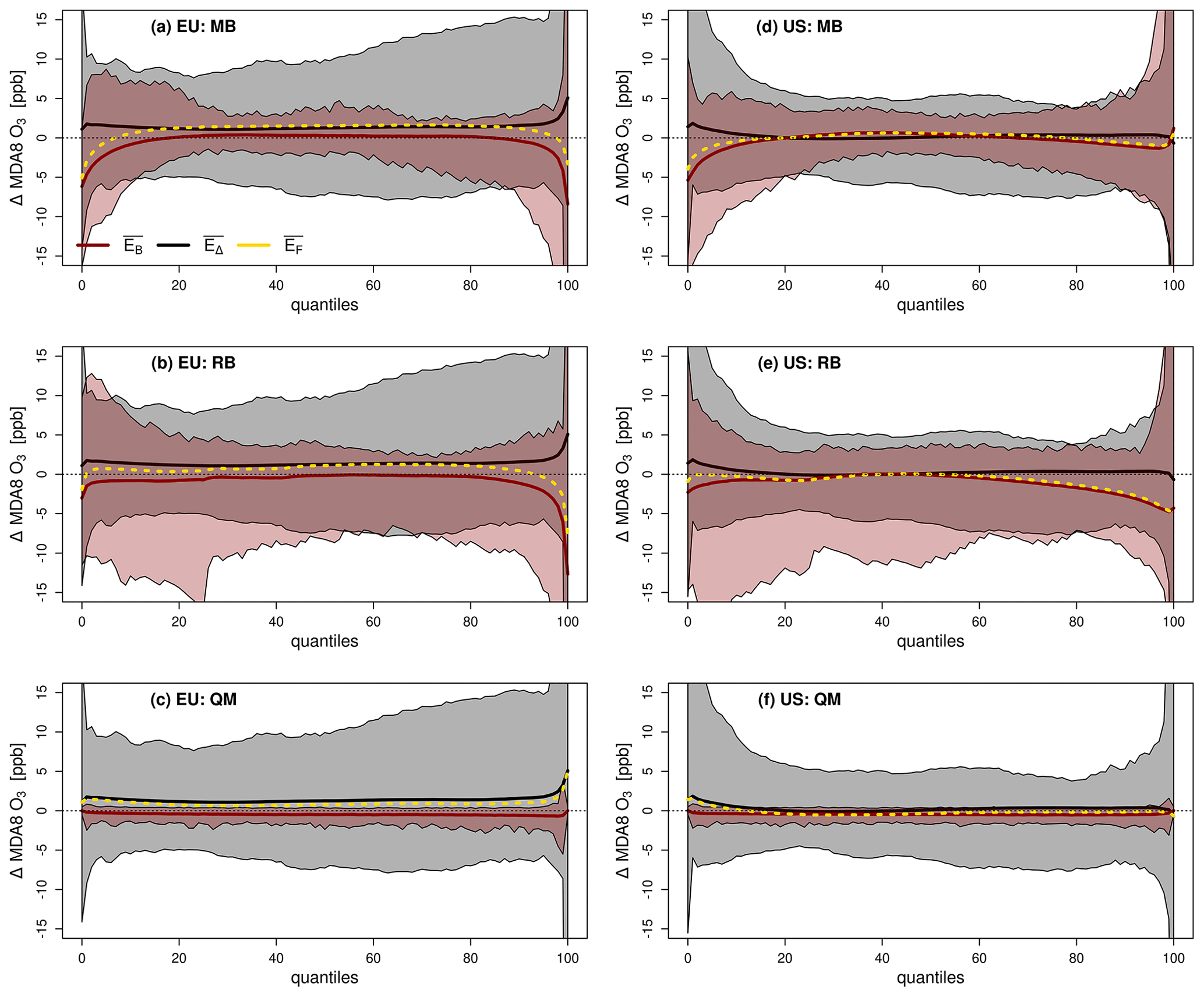
Figure 5 Error components of the CESM2-WACCM6 model during the evaluation period for the MB (a, d), RB (b, e) and QM (c, f) methods in the EU (left column) and the US (right column) domains. The red shading gives the minimum to maximum range, and the solid red line is the domain average of the residual bias in the base period (E_B). The grey shading gives the minimum to maximum range, and the solid black line is the domain average of the differences in the change between the base and evaluation period of the raw model and observations (E_Δ). The resulting domain average error of the evaluation period (E_F) is indicated by the dashed yellow line (note that for the DC method E_B=0 and hence E_F= E_Δ).

3.4 The influence of meteorology on the bias in the CESM2-WACCM6 ensemble

Having illustrated the MDA8 O₃ biases of various CMIP6 models, the performance of various statistical bias techniques and the influence of the model response to changes in, for instance, emissions on the performance of bias correction, we turn our focus to shedding light on the underlying cause of biased MDA8 O₃ model outputs. To this end, we analyze the 13 members of the CESM2-WACCM6 ensemble in more detail in order to examine the individual realizations for consistency as well as to find a possible dominant cause for the bias in the modeled surface ozone fields. Here, two likely prime candidates exist: (1) issues with the sensitivity in chemical mechanisms to local and/or regional precursor emissions (note that anthropogenic emissions are consistent across individual models) and (2) issues in meteorology simulated by the free-running CCM. For the latter, we further include three key climatological drivers of ozone production/accumulation in our analysis, i.e., daily maximum temperature (TSMX), daily average downwelling shortwave radiation (FSDS) and daily average wind speed (WSPD), in order to discern whether the bias is predominantly driven by sensitivity to meteorology or to chemistry. As chemical covariates, we include monthly averages of NO, NO₂ and HCHO; the latter we consider a bulk proxy for VOCs (e.g., Shen et al., 2019; Zhu et al., 2017).

Figures 6 and 7 illustrate the PDFs of MDA8 O₃, NO, NO₂, HCHO, TSMX, FSDS and WSPD for the individual ensemble members during spring and summer in 2005–2009 (the PDFs for 2010–2014 are shown in Supplement Figs. S11 and S12). MAM and JJA MDA8 O₃ (Fig. 6a and e) shows a very similar distribution across ensemble members for both domains. For example, the median MDA8 O₃ value across ensemble members ranges roughly between 50 to 52 ppb (MAM) and 45 to 47 ppb (JJA) in the EU. For the US, the median MDA8 O₃ values were found to be slightly higher than in the EU, but the differences within the ensemble lie in the same narrow range (53 to 55 ppb for MAM and 54 to 55 ppb for JJA). Similarly, compact PDFs across the ensemble are found for NO, NO₂ and HCHO. Interestingly, differences emerge for HCHO in the US but not in Europe, which represents a larger influence of biogenic emissions.

Similar results are found for the meteorological variables. Although slight variations occur for surface temperature, radiation and wind speed (which one would expect from a model generating its own meteorology), the PDFs are widely homogenous across the ensemble, thereby explaining the similarity of surface ozone distributions within the ensemble in both domains (as all ensemble members are driven by the same set of precursor emissions). The analysis of the MDA8 O₃, NO, NO₂, HCHO, TSMX, FSDS and WSPD distributions over the second time period (2010–2014; Figs. S11 and S12) yields similar results, thereby providing confidence in the robustness of our findings.

The strong similarity across ensemble members indicates that the MDA8 O₃ bias identified in CESM2-WACCM6 most likely stems from sensitivities in the chemical mechanism and/or emissions and not from meteorological drivers and their variability. As the models use the same anthropogenic emissions, the differences are more likely to stem from the chemistry, which could include different mixes of emitted VOCs. Previous research has shown that temperature biases are rather small and that a significant overestimation of the temperature in the troposphere occurs solely in the Southern Hemisphere polar region, a region which is not investigated here (Danabasoglu et al., 2020; Gettelman et al., 2019). Nevertheless, we note that small deviations in temperature have been found to explain biases of 5–15 ppb for surface O₃ in former model generations (Rasmussen et al., 2012). While the presented ensemble analysis is, due to data availability, only possible for CESM2-WACCM6, the results provide a first-order estimate of the dominant model component responsible for surface ozone biases. Future work should confirm that this finding holds for other global models, and thus an ensemble strategy for model experiments is recommended for future model intercomparison activities such as CCMI and CMIP.

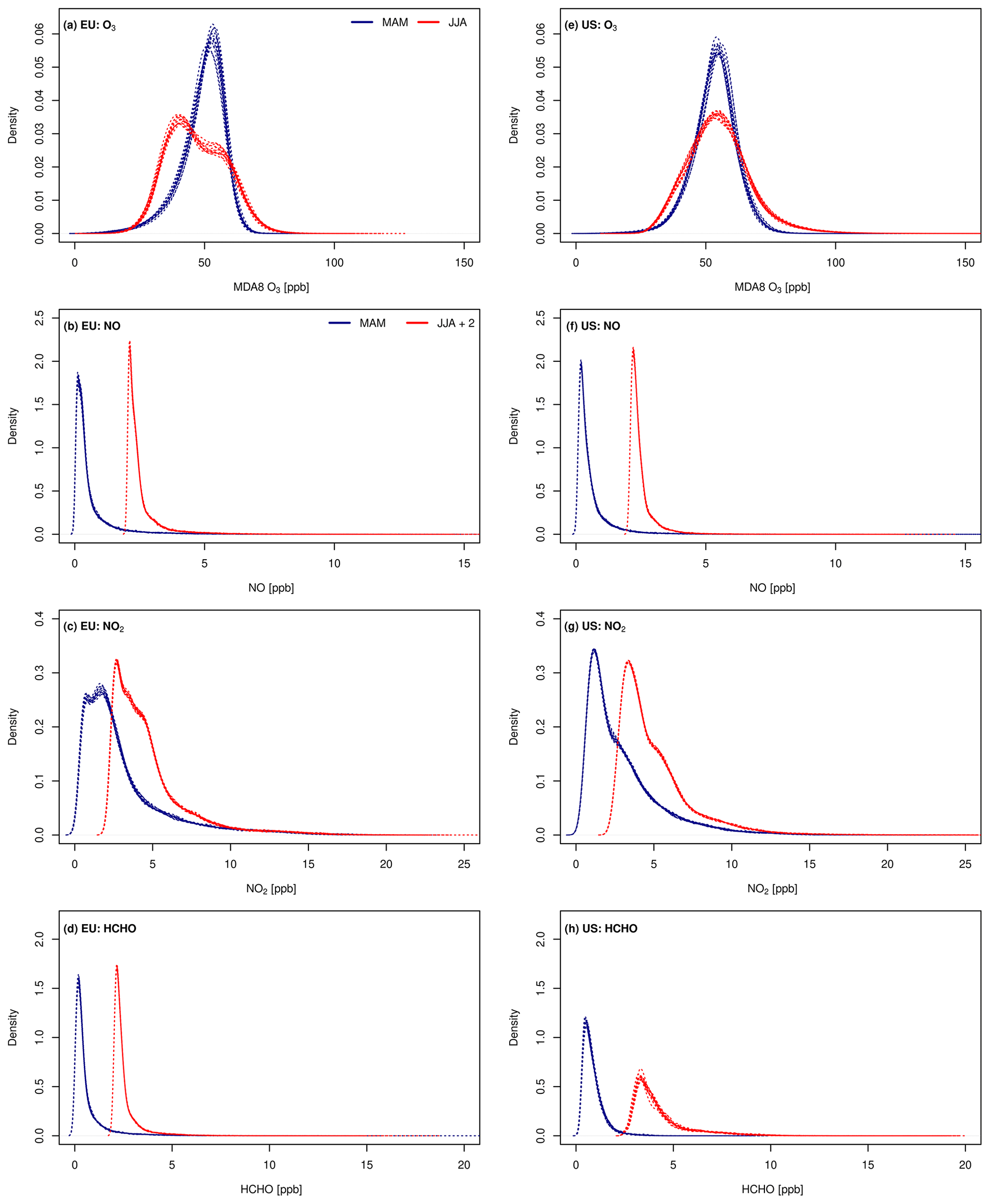
Figure 6 CESM2-WACCM6 spring (MAM) and summer (JJA) PDFs of (a) MDA8 O₃, (b) NO, (c) NO₂ and (d) HCHO for the EU domain in 2005–2009. Panels (e)–(h) are as (a)–(b) but for the US domain. Note that a value of 2 has been added to summertime concentrations of NO, NO₂ and HCHO to allow for visual separation of the seasonal PDFs.

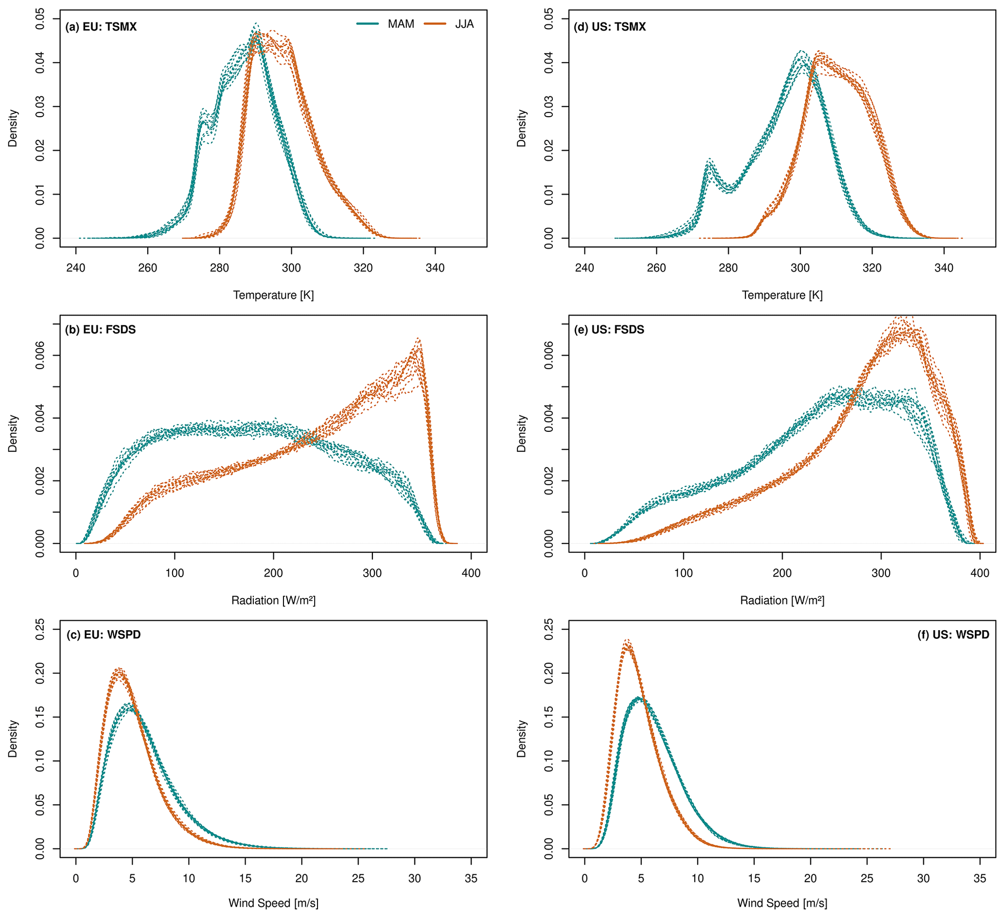
Figure 7 CESM2-WACCM6 spring (MAM) and summer (JJA) PDFs of (a) TSMX, (b) FSDS and (c) WSPD for the EU domain in 2005–2009. Panels (d)–(f) are as (a)–(c) but for the US domain.

4 Summary and conclusions

In this study, we evaluate the bias in surface ozone burdens for four global CCMs contributing to CMIP6 (EC-Earth3, CESM2-WACCM6, GFDL-ESM4 and UKESM1-0-LL) and present the first comprehensive comparison of the performance of four different statistical bias correction techniques to derive CCM-based ozone metrics with relevance for public health and policy. While all models show biases when compared to observations, the bias magnitude of the raw, uncorrected MDA8 O₃ outputs differs strongly within the pool of models analyzed.

The evaluation of the four bias correction techniques for the base period (2005–2009), where techniques are tuned to observations, illustrates that all methods are capable of lowering the bias. The MB and RB methods, however, are less accurate when contrasted with the results obtained from the DC or QM approaches. Furthermore, when applying the MB and RB methods, the model output fields might even be overcorrected for individual grid cells; i.e., the resulting ozone distributions might become biased low. This is not surprising as both techniques apply a single average value for the correction of the whole distribution function, which is a disadvantage – especially when it comes to the tails of the distribution – if the bias is not constant across the ECDF.

The independent evaluation of the four techniques over the second time period (2010–2014) focusing on the bias correction of model projections yields less distinct results. Although the model-to-observation agreement is improved for all MDA8 O₃ metrics in the corrected models compared to their raw counterparts, no single, optimal correction technique can be identified. Our results illustrate that technique performance depends strongly on the model selected and its MDA8 O₃ evolution over time and thus on the response to boundary condition changes. This at first surprising result, however, can be explained by the examination of the composition of the residual model error.

The residual error for future projections is comprised of two parts: (1) the residual error of the base period E_B and (2) the error attributable to the model response to changes in boundary conditions (emissions, climate, etc.) between both time periods, E_Δ. The magnitude of E_Δ was found to exert a dominant influence on the overall correction performance, which raises some concerns regarding the robustness of model responses and thus the reliability of model projections (not only in the context of surface O₃). In contrast to E_Δ,E_B depends on the quality of the initial base period bias correction. Here, our results clearly show that E_B is substantially larger for the MB and RB methods than for the QM and DC methods. When applying the correction techniques, E_Δ and E_B might compensate for individual grid cells, resulting in a low residual bias. On the contrary, the strong performance for the base period obtained with the QM and DC approaches is attributable to a very low E_B, which might deteriorate in projections if E_Δ is large. Thus, we conclude that under the assumption of an adequate model response to changing boundary conditions (and thus low E_Δ), the QM and DC methods outperform the MB and RB techniques. If a decision has to be made as to whether the DC or QM approach is used for bias correction, given that differences between the results obtained with both techniques are negligible, we would argue for DC correction due the comparably easy numerical implementation.

To obtain further insights into the root cause(s) of the surface ozone bias in models, we explored the MDA8 O₃ output of the 13-member CESM2-WACCM6 ensemble together with information on NO, NO₂ and HCHO and key meteorological covariates for ozone production, i.e., daily maximum temperature, daily mean incoming shortwave radiation and daily mean wind speed. Here, our analysis showed only small variations within the CESM2-WACCM6 ensemble for core meteorological drivers (and chemical covariates) of surface ozone. This suggests, given that emissions are consistent across models, a dominant influence of the chemical mechanism on the bias in the O₃ fields rather than a prominent role of model meteorology. Investigating whether this finding can be generalized to other CCMs requires future community efforts in the provision of additional ensemble simulations for individual CCMs contributing to the CCMI or CMIP frameworks.