Extensive coverage of ultrathin tropical tropopause layer cirrus clouds revealed by balloon-borne lidar observations

Tropical tropopause layer (TTL) clouds have a significant impact on the Earth's radiative budget and regulate the amount of water vapor entering the stratosphere. Estimating the total coverage of tropical cirrus clouds is challenging, since the range of their optical depth spans several orders of magnitude, from thick opaque cirrus detrained from convection to sub-visible clouds just below the stratosphere. During the Strateole-2 observation campaign, three microlidars were flown on board stratospheric superpressure balloons from October 2021 to late January 2022, slowly drifting only a few kilometers above the TTL. These measurements have unprecedented sensitivity to thin cirrus and provide a fine-scale description of cloudy structures both in time and in space. Case studies of collocated observations with the spaceborne Cloud-Aerosol Lidar with Orthogonal Polarization (CALIOP) show very good agreement between the instruments and highlight the Balloon-borne Cirrus and convective overshOOt Lidar's (BeCOOL) higher detection sensitivity. Indeed, the microlidar is able to detect optically very thin clouds (optical depth $\mathit{\tau }<\mathrm{2}\times {\mathrm{10}}^{-\mathrm{3}}$) that are undetected by CALIOP. Statistics on cloud occurrence show that TTL cirrus appear in about 50 % of the microlidar profiles and have a mean geometrical depth of 1 km. Ultrathin TTL cirrus ($\mathit{\tau }<\mathrm{2}\times {\mathrm{10}}^{-\mathrm{3}}$) have a significant coverage (23 % of the profiles), and their mean geometrical depth is 0.5 km.

1 Introduction

In the tropics, the transition between the troposphere and stratosphere occurs in a vertically extended layer (14 to 18.5 km) sharing characteristics from both the troposphere and the stratosphere: the tropical tropopause layer (TTL; Fueglistaler et al., 2009; Randel and Jensen, 2013). Most of the air entering the stratosphere makes its way through the TTL along the ascending branch of the Brewer–Dobson circulation (Brewer, 1949). The TTL is then often referred to as the “gate to the stratosphere”. On their way up, air masses encounter extremely low temperatures at the cold point tropopause (CPT; ∼ 17 km, ∼ 190 K) that freeze-dry a great part of their water content and are ultimately responsible for the dryness of the lower stratosphere (Holton et al., 1995). Although water vapor concentration in the stratosphere is very low (∼ 5 ppmv), it has a significant radiative impact on the whole climate system (Solomon et al., 2010) and plays a major role in stratospheric chemistry (Fueglistaler et al., 2009), yet its evolution is not accurately represented in today's climate models. It is thus necessary to get a better understanding of the various TTL processes (transport, dynamical, radiative, and microphysical processes) modulating the amount of water vapor and other trace gases that eventually reaches the stratosphere.

At the heart of the interplay between those processes, TTL clouds have been subject to numerous studies in the past few decades. Thanks to their high vertical resolution and unique sensitivity to tenuous clouds, lidar observations have long been used to characterize tropical clouds, operated from the ground (e.g., Platt et al., 1984, 1987) or from research vessels (e.g., Fujiwara et al., 2009), but their spatial coverage is limited, and they suffer from being potentially blinded by opaque clouds between the ground and the upper troposphere. Passive spaceborne observations (either radiometers (e.g., Prabhakara et al., 1988) or solar occultation measurements (e.g., Wang et al., 1994)) have broadened the picture, providing almost global observations, but they lack sensitivity and resolution to fully capture the TTL cloud coverage. Since the pioneer Lidar In-space Technology Experiment mission (LITE; Winker and Trepte, 1998), spaceborne lidars have overcome these limitations. For the past 17 years, the Cloud-Aerosol Lidar with Orthogonal Polarization (CALIOP) on board the Cloud-Aerosol Lidar and Infrared Pathfinder Satellite Observation (CALIPSO) has provided continuous observations that have led to a great deal of cloud studies (Yang et al., 2010; Martins et al., 2011; Iwasaki et al., 2015; Sourdeval et al., 2018). This mission recently ended on 1 August 2023. CALIOP's cloud observations have intensively been evaluated against other types of measurements, from ground-based lidars (Thorsen et al., 2011) to geostationary weather satellites (Sèze et al., 2015). Recent airborne campaigns such as the NASA Airborne Tropical TRopopause EXperiment (ATTREX; Jensen et al., 2017) have enabled the in situ characterization of thin TTL cirrus (Krämer et al., 2020). A noteworthy result from aircraft data was the characterization of a systematic relationship between TTL clouds and equatorial and gravity waves (Kim et al., 2016). This finding was later confirmed with spaceborne (Chang and L'Ecuyer, 2020) and more recently with balloon-borne observations (Bramberger et al., 2022).

Long-duration stratospheric balloons constitute an invaluable platform to better characterize cloud distribution. Since the balloon is slowly drifting with air, it is able to capture the fine-scale spatial variability of the underlying cloud scene. Here, we introduce the first observations from the Balloon-borne Cirrus and convective overshOOt Lidar (BeCOOL; Ravetta et al., 2020). The nadir-looking BeCOOL system has a viewing geometry comparable to CALIOP but benefits from a significantly higher signal to noise ratio (SNR) in the TTL and upper troposphere thanks to the long integration time allowed by the low speed of the balloon and the small distance to the observed clouds. BeCOOL was recently flown for the first time on board three superpressure balloons (SPBs) in the framework of the Strateole-2 project (Haase et al., 2018; Corcos et al., 2021; Bramberger et al., 2022). The SPBs were launched from Seychelles and traveled up to the middle of the Pacific Ocean at about 20.5 km (50 hPa) between October 2021 and January 2022, gathering 700 nighttime hours of high-resolution lidar profiles.

The article is organized as follows: Sect. 2 presents the different data sets and the cloud classification. In Sect. 3, three case studies of collocated BeCOOL and CALIOP observations are analyzed to contrast the two instruments, their sampling, and detection capability. Section 4 is dedicated to a statistical description of the balloon-borne cloud data and a statistical comparison with spaceborne lidar data. Conclusions and perspectives are in Sect. 5.

2 Lidar data sets

2.1 Balloon-borne lidar data

BeCOOL nighttime observations were gathered during the first Strateole-2 field campaign, from 20 October 2021 to 26 January 2022. Among the 17 balloons released during the campaign, 3 were carrying BeCOOL microlidars. They were successively launched from Seychelles and drifted eastward at an altitude of about 20.5 km near the Equator; their trajectories are shown in Fig. 1a. The main characteristics of the flights are presented in Table 1, and a summary of the technical specifications of the BeCOOL microlidar is presented in Table 2.

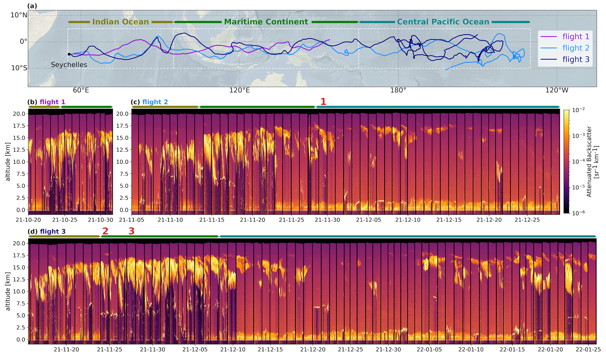
Figure 1 (a) Trajectories of the three balloons carrying BeCOOL during the first Strateole-2 scientific campaign. The dashed white boxes show the three studied regions; (b–d) lidar curtains (time vs. altitude, attenuated backscatter) for the three flights (concatenated nights of observations: apart from the thin vertical black lines, daytime has been removed for the sake of readability). Overflown regions are color-coded on top of the curtains. The red numbers (1, 2, and 3) highlight the three case studies presented in Sect. 3.

Table 1 Main characteristics of the three Strateole-2 flights carrying the BeCOOL microlidar; $\stackrel{\mathrm{‾}}{z}$ is the mean altitude above sea level and $\stackrel{\mathrm{‾}}{\left|\mathbf{u}\right|}$ the mean ground speed of the balloon.

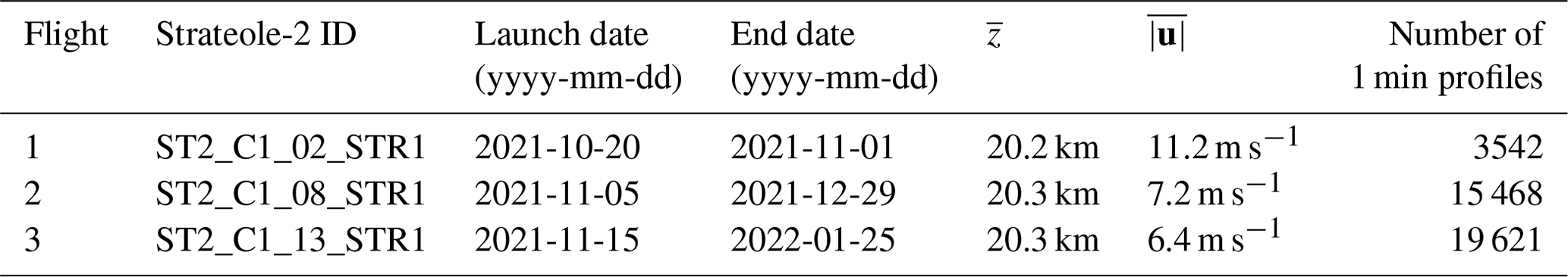
Table 2 Overview of the main characteristics of the BeCOOL and CALIOP lidars.

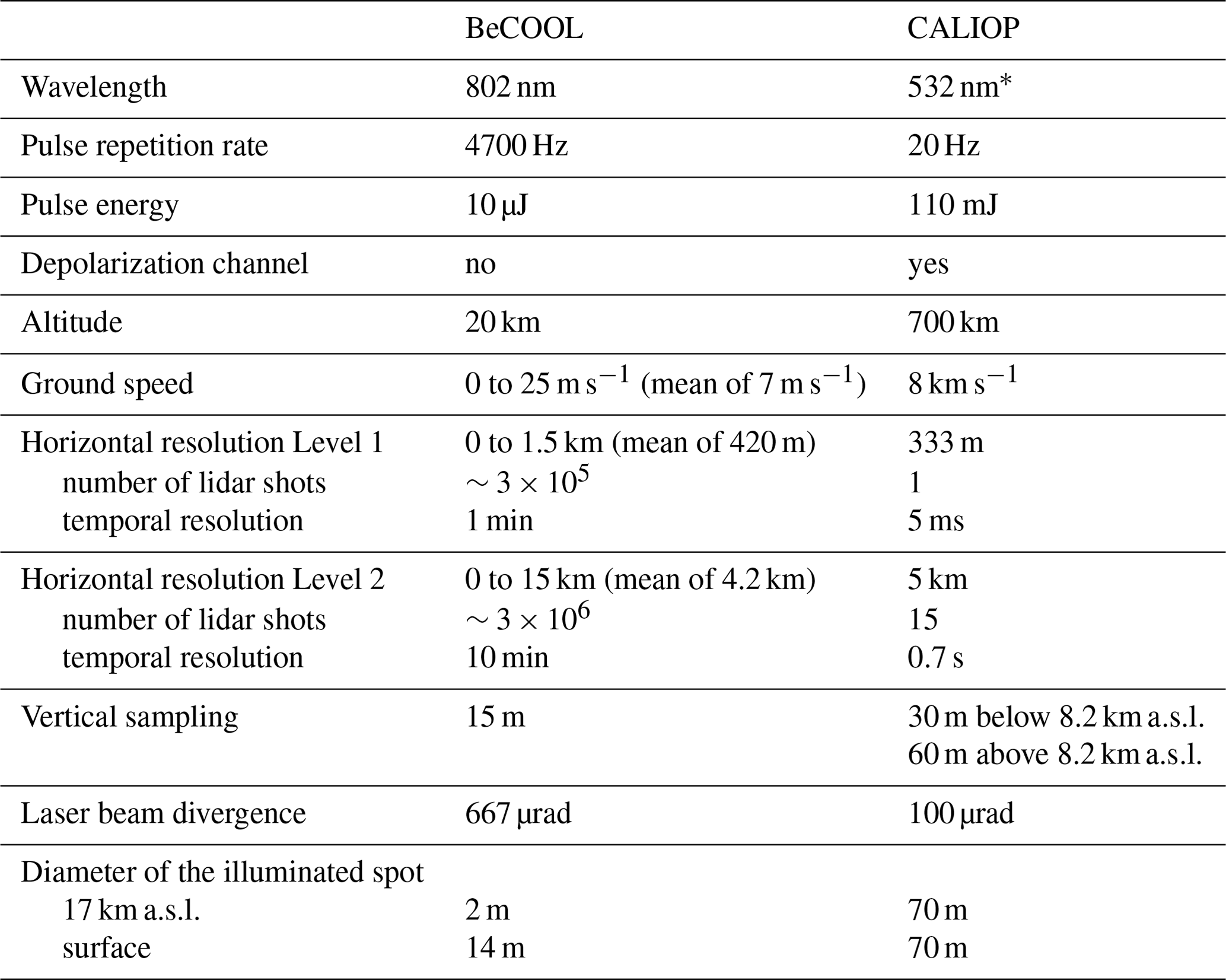
^∗ CALIOP's 1064 nm channel is not used in this study.

Overall, 38 631 lidar profiles have been measured at the native 1 min resolution. Each raw lidar profile is corrected from the radiometric background derived from the tail of the signal, then multiplied by the squared range to account for the geometrical dilution of the laser power. For each BeCOOL instrument, an empirical correction of the lidar overlap function has been constructed from a set of clear-sky observations and synthetic pure molecular lidar profiles derived from ERA5 meteorological fields. Every single lidar profile is first corrected for this overlap effect then normalized upon ERA5 using a 1 km thick clear-sky layer above the uppermost clouds, between 1 and 2 km below the lidar, assuming that pure molecular signal prevails in this normalization interval. These normalized lidar profiles are usually called “attenuated backscatter” and are referred to as Level 1.

Geometrical and optical properties of clouds (Level 2) are retrieved after averaging consecutive profiles over 10 min to improve the SNR. Detection of clouds is semi-automated; every profile is manually checked after a first round of automated detection. Cloud optical depths are then retrieved using the classical Klett–Fernald inversion method (Fernald et al., 1972; Klett, 1981), which relies on the particular extinction to backscatter ratio (lidar ratio). Quite similarly to what is done for CALIOP, this quantity can be iteratively constrained for the thicker semi-transparent clouds that significantly attenuate the lidar beam. These constrained retrievals need to be further corrected for multiple scattering (Platt, 1973). BeCOOL's multiple-scattering correction factor η=0.88 has been determined as the appropriate scaling factor that reconciles BeCOOL's “apparent” and CALIOP's “true” optical depth distributions for constrained retrievals. The optical depths of the thinner clouds are retrieved using an a priori lidar ratio chosen as the most frequent value from CALIOP's constrained retrievals over the same period and region at the altitude of the middle of the cloud. The estimated relative uncertainty in these retrievals increases when the optical depth decreases. It is below 10 % for clouds with an optical depth larger than 0.1, below 50 % for clouds with an optical depth larger than 0.01, and much larger (up to 90 %) for the optically thinnest clouds. A comprehensive description of the instrument and the different levels of processing, along with an analysis of their uncertainties, will be detailed in another article.

Figure 1 shows the trajectories of the three flights and the lidar curtains (time vs. altitude) of attenuated backscatter and reveals a large variety of different cloud scenes. Intense surface echos (mainly the ocean surface) are seen in 86 % of the profiles. The lidar beam is fully attenuated by opaque clouds otherwise. In profiles reaching the surface, the ubiquitous aerosol-rich boundary layer generally occupies the lowest 2.5 km along with frequently occurring low-level clouds (cumulus and stratocumulus). Geometrically thin (a few hundred meters), horizontally extensive mid-level clouds are often found above, below 10 km, mainly between 5 and 8 km; they typically have large backscatter and are likely pure liquid or mixed-phase clouds. Above 10 km are pure ice clouds: cirrus and deep convective clouds. The clouds' vertical structure can be fully resolved up to an optical depth ${\mathit{\tau }}_{max}\simeq \mathrm{3}$, a threshold value depending on the energetic conditions and optical efficiency of the instrument, which both vary with thermal conditions on board the gondola. Clouds thicker than this appear opaque (the lidar beam is fully attenuated before reaching the bottom of the cloud), and only their upper part can be resolved. Typically, deep convective clouds have a large vertical extent that cannot be accurately inferred from BeCOOL observations.

For the purpose of this study, the area covered by the balloons has been zonally divided into three regions: the Indian Ocean (55 to 95° E), Maritime Continent (95 to 165° E), and central Pacific Ocean (165 to 230° E). There is a striking contrast between very cloudy profiles over the Indian Ocean and Maritime Continent, with frequent deep convection, and clear-sky conditions over the central Pacific Ocean in the second part of flights 2 and 3.

We built a classification of cloud profiles for the BeCOOL data set. Clouds are first classified using a set of threshold values on their top and base altitude. Cirrus clouds are here defined as all clouds with a base altitude lying above 10 km (i.e., temperatures below the glaciation threshold of supercooled droplets at about 240 K) and are then sub-classed as TTL cirrus if their base altitude is over 14 km. Convective clouds are here defined as opaque clouds (totally attenuating the lidar beam) with a top altitude lying above 10 km. Mid-level clouds have a top altitude between 5 and 10 km. The last class gathers clouds that do not fit previous requirements, with a top altitude above 10 km and base altitude below, sharing characteristics from both cirrus and mid-level clouds. This classification is somewhat restrictive in the case of deep convection, since mostly the core of convective cells will be flagged in this category, while a large part of the convective anvils will be classified as cirrus as long as BeCOOL's lidar beam goes through and the cloud base is above 10 km.

A profile classification has been built from this cloud classification. Clear sky is defined as profiles with no detected cloud above 5 km, since low-level clouds and the planetary boundary layer are not considered in this study. Deep convection gathers profiles exhibiting any convective clouds, regardless of the presence of cirrus on top of it. Cirrus only and mid-level clouds only stand for profiles where only such types of clouds are detected above 5 km. The last class, mixed multilayered scenes, gathers the other profiles, usually exhibiting a complex overlay of cirrus and mid-level clouds.

Further classification of cirrus layers is performed based on their optical depth: thin cirrus have an optical depth below 0.1, which is about the detection lower bound for passive radiometers (McFarquhar et al., 2000); sub-visible clouds have an optical depth $\mathit{\tau }<\mathrm{3}\times {\mathrm{10}}^{-\mathrm{2}}$, a classical value from Sassen et al. (1989); and ultrathin cirrus have an optical depth $\mathit{\tau }<\mathrm{2}\times {\mathrm{10}}^{-\mathrm{3}}$ (which is about the detection threshold of CALIOP; see Sect. 4).

2.2 Spaceborne lidar data

BeCOOL is compared to the CALIOP spaceborne lidar using the Level 2 Cloud and Aerosol merged product with a 5 km horizontal resolution, version 4.21 (Young et al., 2018). This data set reports optical and geometrical properties of detected clouds or aerosol layers along the satellite track. When CALIOP lidar curtains are displayed, the figures are generated using the Level 1 version 4.11 attenuated backscatter product (Kar et al., 2018). In this study, only the 532 nm channel is used. The main technical specifications of the CALIOP lidar, along with BeCOOL's, are presented in Table 2.

While CALIOP flies at ∼ 8 km s⁻¹, achieving its native $\mathrm{1}/\mathrm{3}$ km horizontal resolution from a single lidar shot, BeCOOL flies 1000 times slower, which allows us to integrate individual lidar shots for a whole minute, considerably enhancing the SNR. This speed difference also implies that CALIOP provides an almost-instantaneous description of cloudy structures at synoptic scale, while the temporal and spatial evolution of the underlying scene is entangled in BeCOOL's observations. BeCOOL's laser divergence (667 µrad) is significantly higher than CALIOP's (100 µrad), meaning that BeCOOL's high SNR in the near field decreases toward the surface due to geometric power dilution, whereas this effect can be neglected for CALIOP.

Following Reagan et al. (2002), we assume that the optical depths retrieved at the 802 nm (for BeCOOL) and 532 nm (for CALIOP) wavelengths are comparable, i.e., that the scattering particles are larger than 5–8 µm such that there is only weak wavelength dependency of Mie scattering.

During the campaign, CALIOP crossed the Equator around 02:30 local time (LT). Originally crossing the Equator at 01:30 LT as part of the Afternoon Constellation (A-train), CALIPSO was moved to a lower orbit in 2018 to join CloudSat (Braun et al., 2019). As CALIPSO's fuel reserves were coming to an end, the satellite had been experiencing an orbital drift, which explains the 02:30 LT crossing time during the campaign instead of the usual 01:30 LT.

3 Case studies of BeCOOL and CALIOP collocated observations

Three case studies of collocated BeCOOL and CALIOP measurements are now presented in order to compare the two instruments at coincidence time and highlight their complementarity due to the fundamental differences mentioned in the previous section. The case studies correspond to different cloud scenes: a thick (anvil) cirrus, a thin cirrus, and deep convection. To contextualize the cloud scene around lidar observations, we use the NOAA/NCEP GPM-MERGIR brightness temperature data in the atmospheric window (∼ 11 µm). This product combines observations from four geostationary satellites and provides a global coverage with spatial resolution of 4 km and temporal resolution of 30 min (Janowiak et al., 2001).

Figures 2, 3, and 4 present lidar curtains from the two instruments along with the GPM-MERGIR brightness temperature map closest to the coincidence time, with a size of 5° × 5°. CALIOP's curtain resolution below 8.2 km a.s.l. has been degraded to 1 km horizontally and 60 m vertically, which is the native resolution above 8.2 km a.s.l. BeCOOL's curtains are displayed for the whole nights (roughly 11 h of observations), starting around 18:00 LT and ending around 05:30 LT, covering a horizontal distance of 200 to 500 km along the balloon's track depending on the wind speed. Each CALIOP's curtain is 570 km long (dashed line on the maps), covered in about 82 s.

As previously stated, CALIOP's observations are almost instantaneous and can be compared with a single brightness temperature map from GPM-MERGIR, with latitude appearing as a natural coordinate for CALIOP, while time is the natural coordinate for BeCOOL, which can only be compared with successive brightness temperature maps. Hourly maps for the three case studies are presented in the Appendix, Figs. B1, B2, and B3.

3.1 First case study: thick cirrus cloud

Figure 2 shows an excellent coincidence that happened on 29 November 2021 over the Pacific Ocean (∼ 4° S, 172° E) for the second BeCOOL flight. The satellite track crossed the balloon track less than 1 km away from it. The balloon covered 430 km during this night. There is perfect agreement between the two lidars at the coincidence time: they both capture a thick cirrus cloud extending from 12 to 16 km over two mid-level clouds, around 5 and 7 km, with very small vertical extent. Both lidars' profiles around the coincidence time are displayed in the Appendix in Fig. A1. CALIOP's curtain shows that this thick cirrus is embedded in a larger-scale thinner laminar cirrus extending vertically from 14 to 16 km and horizontally all along the 570 km track displayed here. The brightness temperature map at 15:00 UTC reveals the horizontal structure of this thick cirrus, centered on the coincidence spot and with an apparent radius of ∼ 100 km. BeCOOL's curtain and the hourly brightness temperature maps in Fig. B1 allow us to follow the temporal evolution of the scene under the balloon: from the beginning of the night up to 13:00 UTC, a thin and laminar cirrus vertically extending between 15 and 17 km, with an optical depth of 0.08, is overflown; this cirrus then thickens to extend vertically from 12 to 16 km, reaching an optical depth of 0.5. The balloon follows the thick cloud for the second part of the night as they are both advected eastward.

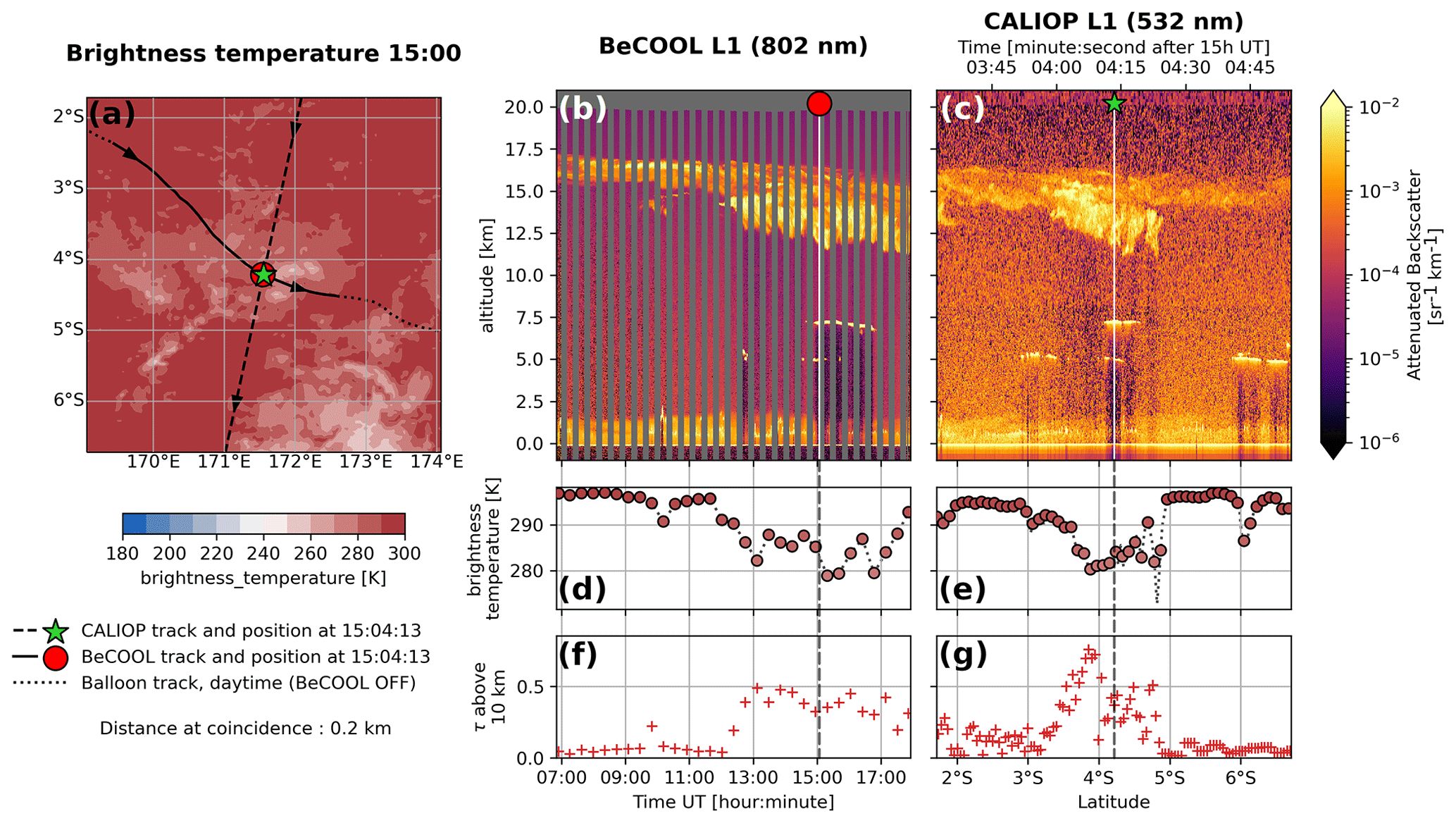
Figure 2 First case study: thick cirrus cloud, 29 November 2021. (a) The 11 µm brightness temperature map at 15:00 UTC, (b) BeCOOL L1 curtain (along the solid line on the map), (c) CALIOP L1 curtain (along the dashed line on the map), (d, e) time series of brightness temperature under the balloon and the satellite, (f, g) time series of optical depth τ above 10 km retrieved from BeCOOL and CALIOP.

The brightness temperature (BT) below both instruments (Fig. 2d–e) exhibits high values (almost 300 K) above the thin part of the cloud, between 07:00 and 09:00 UTC in Fig. 2b and between 2 and 3° S in Fig. 2c. BT drops down to 280 K above the thicker part of the cloud, after 13:00 UTC in Fig. 2b and around 4° S in Fig. 2c. Clouds' contribution to upward thermal flux increases with optical depth, actually lowering the flux and revealing the thermal contrast between low temperatures at cloud level and higher temperatures below. BT (Fig. 2d–e) and total cloud optical depth above 10 km (Fig. 2f–g) are thus quite anti-correlated: $r=-\mathrm{0.88}$ along BeCOOL's track and $r=-\mathrm{0.72}$ along CALIOP's. These correlations would be more significant without the presence of mid-level clouds around 5 and 7 km, which are not accounted for in the total cloud optical depth above 10 km but further lower the BT (e.g., Fig. 2e at 6° S).

At coincidence, the retrieved cirrus' optical depths are 0.32 for BeCOOL and 0.37 for CALIOP, which is quite good agreement. This discrepancy is well within the range of uncertainties and mainly related to the strong spatial variability of this thick cirrus, which can be seen both on lidar curtains and on the lidar profiles displayed in Fig. A1.

3.2 Second case study: thin cirrus clouds

The second case study (Fig. 3) happened for the third BeCOOL flight off the east coast of the island of Sumatra, Indonesia (∼ 3° N, 97° E; distance at coincidence: 10.4 km), and corresponds to collocated observations of a very thin TTL cirrus, which is only partially reported in CALIOP Level 2 data. BeCOOL's curtain in Fig. 3 clearly reveals a thin cloudy layer above 17.5 km, first fading out from the beginning of the night until 14:00 UTC, then reappearing from 15:30 UTC and slowly thickening until 20:00 UTC, reaching up to $\mathrm{5}\times {\mathrm{10}}^{-\mathrm{3}}$ optical depth. This horizontally homogeneous, geometrically and optically very thin cirrus layer appears to fit the description of ultrathin tropical tropopause clouds (UTTCs) reported by Peter et al. (2003). In CALIOP's curtain, this cloud can be identified by the human eye around 17.5 km in the 532 nm total attenuated backscatter (Fig. 3c). However, it is only reported in CALIOP L2 for about 10 s around coincidence. It was detected after a horizontal averaging of 80 km, the last step of the algorithm designed to improve SNR in order to detect tenuous features, but its horizontal extent could likely have been better constrained with even more extensive horizontal averaging. Given the limitation of the CALIOP L2 algorithm for such a case and for the sake of a fair comparison of the instrument capabilities, we manually retrieved the UTTC optical depth from CALIOP L1. We first improve the SNR by applying a horizontal rolling mean over a 80 km window. Then, we retrieve the cirrus optical depth at three latitudes: 4.5, 3, and 1.5° N, keeping the same lidar ratio (21.8 sr) and multiple scattering factor η (0.77) as reported in CALIOP L2 for the central part of this cloud. This cirrus' optical depth is $\mathrm{8.3}\times {\mathrm{10}}^{-\mathrm{4}}$ at 5° N, increasing to $\mathrm{4.0}\times {\mathrm{10}}^{-\mathrm{3}}$ at 3° N (coincidence) then decreasing to $\mathrm{2.2}\times {\mathrm{10}}^{-\mathrm{3}}$ at 1.5° N. At coincidence, the retrieved optical depths from both observations are thus in excellent agreement.

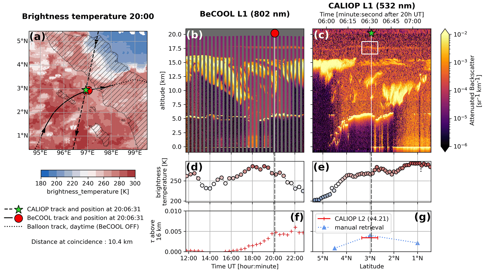
Figure 3 Second case study: thin cirrus cloud, 24 November 2021. (a) The 11 µm brightness temperature map at 20:00 UTC, (b) BeCOOL L1 curtain (along the solid line on the map), (c) CALIOP L1 curtain (along the dashed line on the map), (d, e) time series of brightness temperature under the balloon and the satellite, (f, g) time series of optical depth τ above 16 km retrieved from BeCOOL and CALIOP. The CALIOP L2 operational algorithm partially detects the thin cirrus (white box in (c), red segment in (g)) after a 80 km horizontal averaging and reports a single optical depth value for this 80 km leg around coincidence time: at this resolution, a single point is detected as cloudy, and the CALIOP algorithm is missing most of the cloud.

We can attempt to estimate the horizontal extension of this UTTC assuming that it expands a few hundreds of kilometers along both instruments' tracks: this cirrus could have an area greater than 10⁵ km², which is the order of magnitude observed by Peter et al. (2003) for UTTCs.

Regarding backscattered power, the contrast between this cloud and the surrounding clear sky is about 3 times higher at 802 than 532 nm (due to the strong wavelength dependency of Rayleigh scattering, emphasized by Peter et al., 2003). This is why, in addition to a lower absolute noise level, very thin features are more easily detected with BeCOOL. Such thin layers are sometimes clearer in the depolarization ratio (not shown here) and should have a stronger signature in CALIOP's second channel (1064 nm), but the operational layer detection algorithm only relies on the 532 nm channel for now. Further reprocessing of CALIOP's observations is expected to improve the detection and retrieval of very thin clouds. Vaillant de Guélis et al. (2021) recently introduced a new two-dimensional multi-channel cloud detection algorithm for CALIOP. Preliminary tests on collocated BeCOOL and CALIOP observations over very thin clouds show large improvements in cloud layer detection. Other projects of CALIOP reprocessing rely on machine learning techniques to detect optically thin clouds (Wang et al., 2019).

3.3 Third case study: convective clouds

Figure 4 displays a CALIOP–BeCOOL coincidence which occurred on 27 November 2021 off the southeast coast of the island of Borneo, Indonesia (∼ 4° S, 117° E; distance at coincidence: 72.7 km), for the third BeCOOL flight. CALIOP overflew several convective cells, capturing two events of convection overshooting the main cloud top (white capital letters in Fig. 4a–c). The first one (A) has an apparent diameter of 40 km and seems to be fading out at the time of overpass, having appeared 1 to 2 h before (see the hourly maps in Fig. B2). The second one (B) seems to be popping up right under the satellite and has an apparent diameter of 15 km. The core of this cell is characterized by a very strong backscatter and a small penetration depth: the highest part of this cloud is very dense and optically thick. These two structures clearly overshoot the extensive 17 km cloud top which appears on both curtains and is likely a high-altitude anvil. As shown by the brightness temperature maps, BeCOOL flew all night long around the convective cells, measuring the edges of anvils and revealing the evolution of the multilayered cloud structure. No clear sign of overshoot residual (i.e., cloud above the extensive 17 km deck) appears in BeCOOL data.

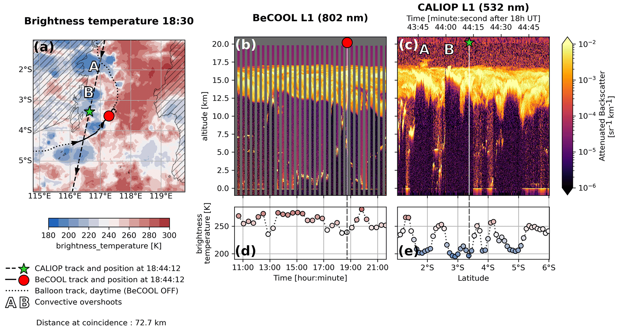
Figure 4 Third case study: convective cloud, 27 November 2021. (a) The 11 µm brightness temperature map at 18:30 UTC, (b) BeCOOL L1 curtain (along the solid line on the map), (c) CALIOP L1 curtain (along the dashed line on the map), (d, e) time series of brightness temperature under the balloon and the satellite. The white capital letters in (a) and (c) show two overshoots detected by CALIOP.

There could be different reasons for this apparent disagreement in overshoot detection. First, it is worth mentioning that overshoots would have different visual aspects in CALIOP and BeCOOL curtains. Assuming a wind difference of 7.5 m s⁻¹ between the balloon and the cloud top (mean value over the Maritime Continent along the three flights, according to ERA5 reanalysis), an overshoot with a size of 40 km would be overflown for about 1.5 h, a duration comparable to its lifetime (Dauhut et al., 2018; Lee et al., 2019). Thus, it is likely that overshoots in BeCOOL curtains will exhibit a different shape (e.g., aspect ratio) compared to CALIOP's and cannot be identified as clearly. Over the whole campaign, we found no obvious observation in BeCOOL's data of an overshoot similar to the protrusion detected by CALIOP in this example. Since convective overshoots are one of the scientific targets of BeCOOL, we further investigated the probability of overflying very deep convection with the balloons using 11 µm brightness temperature (BT) data. We defined a T_overshoot=200 K BT threshold as a proxy for potentially overshooting convection, based on the comparison between CALIOP and BT maps in this case study. Over the Maritime Continent and during the campaign, about 1 % of the pixels of the BT maps have values lower than T_overshoot, whereas such cold pixels are 3 times less likely to occur along the balloon tracks (0.3 % of the observations over this area). Such low frequency of observation of “cold” cloud scenes constitutes a “warm” sampling bias for our three flights. Nevertheless, extending this analysis to all 17 Strateole-2 campaign balloons, we did not find conclusive evidence of a systematic sampling bias, which tends to discard the hypothesis that a dynamical effect (such as flow divergence) prevents the balloon from flying over overshooting tops. Targeting such relatively rare, sparse, and small-scale structures with a limited instrumented fleet may require the use of steerable balloons.

4 Statistical description

4.1 Cloud coverage and scene complexity

A summary of BeCOOL's profile classification over the Maritime Continent and central Pacific Ocean is provided in Table 3. A striking contrast appears between the two regions: over the Maritime Continent, convection is detected in up to 15 % of the profiles, and clear-sky scenes are almost absent (0.2 %). On the contrary, more frequent clear-sky profiles (10 %) and far less convective ones (0.5 %) are found over the central Pacific. Over the central Pacific, 69 % of the profiles present only cirrus and 55 % only TTL cirrus. Over the Maritime Continent, more than half of the profiles correspond to a complex combination of different types of clouds, here reported as mixed multilayered scenes, while we only report 16 % of such profiles over the central Pacific Ocean. Although several types of scenes are gathered in this mixed multilayered class, a great part of them could be somehow related to different stages of convective activity: developing convection, detrainment, and/or precipitation. The campaign took place during the La Niña phase of the El Niño–Southern Oscillation (NCEI, 2023). The strong contrast in convective activity between the Maritime Continent and central Pacific Ocean is typical of this ENSO phase (e.g., Gage and Reid, 1987).

Table 3 BeCOOL main profile classification (percentages of 10 min averaged profiles). Details on this classification can be found in Sect. 2.1.

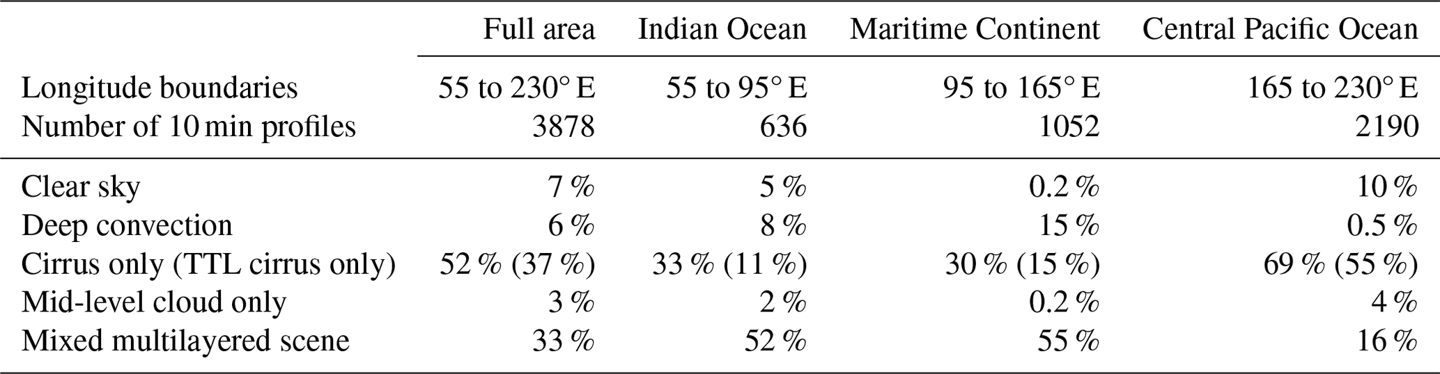
Table 4 Frequency of occurrence of cirrus (cloud base > 10 km) in BeCOOL profiles with different thresholds on optical depth (percentages of 10 min profiles). The bold font stands for TTL cirrus (cloud base > 14 km).

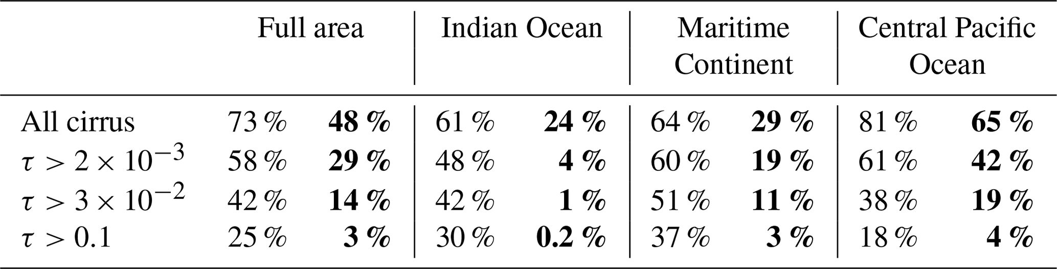
Table 4 summarizes the occurrence of cirrus and TTL cirrus for several optical depth thresholds. Regardless of their optical depth, cirrus are detected in 73 % of all profiles with a small regional contrast: from 61 % over the Indian Ocean to 81 % over the central Pacific Ocean. The regional contrast is more pronounced for TTL cirrus, which are detected in 24 % of the profiles over the Indian Ocean and 65 % over the central Pacific Ocean. The thresholds on optical depth show what would be detected by a less sensitive instrument: CALIOP (τ>0.002), human bare eye (visible cirrus, τ>0.03), and passive radiometers (τ>0.1). The cirrus cloud cover estimate strongly depends on this detection threshold: over the full area, not taking into account the thinnest cirrus clouds (optical depth below $\mathrm{2}\times {\mathrm{10}}^{-\mathrm{3}}$) reduces the total cirrus coverage by 15 % and 19 % for the TTL cirrus only. A passive radiometer insensitive to clouds with an optical depth below 0.1 (for example, on board geostationary satellites) would only detect 1 cirrus out of 3 and 1 TTL cirrus out of 16. Thus, with BeCOOL's sensitivity, the estimated cirrus cover is significantly increased compared to what is derived from spaceborne instruments.

4.2 Optical and geometrical properties of mid- and high-level clouds from BeCOOL and comparison with CALIOP

Statistics of cloud properties (optical depth, top and base altitude) have been compiled for all BeCOOL Level 2 profiles. They are compared with CALIOP nighttime profiles measured during the flight period of the microlidars, over the area covered by the balloons (from −10 to 5° N, 50 to 230° E; dashed white box in Fig. 1). All clouds with a reported base altitude below 5 km have been removed from both data sets to focus on free-tropospheric and TTL clouds. We also excluded deep convective clouds with full attenuation of the beam and removed all non-reliable retrievals from CALIOP's database, i.e., where the extinction_QC flag is greater than 2.

Figure 5 shows histograms of optical depth for clouds detected above 5 km by the two instruments. Excellent agreement between the distributions appears from $\mathrm{2}\times {\mathrm{10}}^{-\mathrm{3}}$ to ∼1, and the frequencies of occurrence both decrease as τ⁻¹. For BeCOOL, this power law is valid down to $\mathit{\tau }\simeq {\mathrm{10}}^{-\mathrm{4}}$, where the distribution reaches a maximum, whereas a clear cutoff appears at a larger optical depth $\mathit{\tau }\simeq \mathrm{2}\times {\mathrm{10}}^{-\mathrm{3}}$ in CALIOP's distribution, below which the cloud frequency sharply decreases. A total of 27 % of the cloud layers detected by BeCOOL have an optical depth below $\mathrm{2}\times {\mathrm{10}}^{-\mathrm{3}}$. They appear in 32 % of the profiles. For CALIOP, such ultrathin clouds only account for 0.5 % of all detected clouds and are reported in less than 1 % of the profiles.

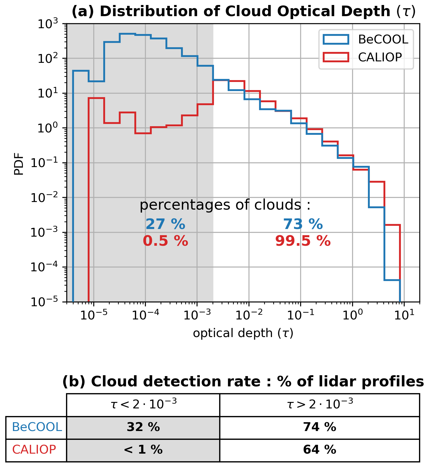
Figure 5 Statistical comparison of cloud layer properties detected by BeCOOL and CALIOP. (a) Probability density functions of optical depth of all clouds above 5 km. The grey shading highlights the low optical depth, up to $\mathrm{2}\times {\mathrm{10}}^{-\mathrm{3}}$, where the distributions diverge. The percentages of detected clouds with an optical depth lower/greater than this $\mathrm{2}\times {\mathrm{10}}^{-\mathrm{3}}$ threshold are reported in the figure. (b) Percentages of lidar profiles showing clouds with an optical depth lower/greater than the $\mathrm{2}\times {\mathrm{10}}^{-\mathrm{3}}$ threshold. Both types of clouds can appear in a single lidar profile.

Figure 6 shows the distributions of cloud top altitude, base altitude, and geometrical depth for all clouds and separately for clouds with an optical depth larger or smaller than a $\mathrm{2}\times {\mathrm{10}}^{-\mathrm{3}}$ threshold. For all clouds, BeCOOL's top altitude distribution shows a sharp mode peaking between 17 and 17.5 km and a wider base altitude distribution peaking between 16.5 and 17 km. The mean geometrical depth is 2 km. Considering only the clouds with an optical depth larger than $\mathrm{2}\times {\mathrm{10}}^{-\mathrm{3}}$, the top altitude distribution remains almost unchanged, with a slightly smoother mode; the base altitude no longer shows any clear mode; and the mean geometrical depth is 2.6 km. Considering only cirrus with an optical depth below $\mathrm{2}\times {\mathrm{10}}^{-\mathrm{3}}$, both top and base altitude distributions show a very sharp mode, peaking between 17.5 and 18 km for the top and between 16.5 and 17 km for the base. Correspondingly, the mean geometrical depth is 490 m. Almost 75 % of those clouds lie within the TTL, and about 50 % have their base above 16.5 km. Hence, not only does BeCOOL perform well in detecting ultrathin TTL clouds (an expected result considering its high SNR in the near field), more importantly, such clouds are detected in more than 20 % of the profiles. Now comparing BeCOOL to CALIOP, a very similar total top altitude distribution is seen, yet with a peak shifted towards lower altitudes, between 16.5 and 17 km. The base altitude distribution of CALIOP does not exhibit any sharp mode and does not extend as high as BeCOOL's, it appears quite uniform between 10.5 and 15.5 km and decreases below, the mean geometrical depth is 2.1 km. Those distributions remain unchanged when considering only clouds with an optical depth larger than $\mathrm{2}\times {\mathrm{10}}^{-\mathrm{3}}$ as they account for 99.5 % of all clouds. The agreement with BeCOOL's top and base altitude distribution is almost perfect for those clouds, although CALIOP's still does not extend as high as BECOOL's. The mean geometrical depth of those clouds is still 2.1 km, which is slightly lower than for BeCOOL, but the distribution does not extend as much to small depths. This difference can be attributed to CALIOP's reception channel photomultiplier tubes, which exhibit a non-ideal transient response when exposed to high levels that tend to lower the apparent base altitude of dense clouds and enhance their apparent geometrical depth (Lu et al., 2013, 2020). This effect appears clearly on CALIOP's profiles in Fig A1: the base of the mid-level cloud around 7 km is hidden in the decaying “noise tail”, while BeCOOL reveals the true geometrical depth of this cloud. This explains the differences between base altitude distributions and geometrical depth, while top altitude distributions show excellent agreement. In striking contrast with BeCOOL, clouds with an optical depth below $\mathrm{2}\times {\mathrm{10}}^{-\mathrm{3}}$ only represent 0.5 % of CALIOP's cloud database, and their top/base altitude distribution is wide and does not show any pronounced mode.

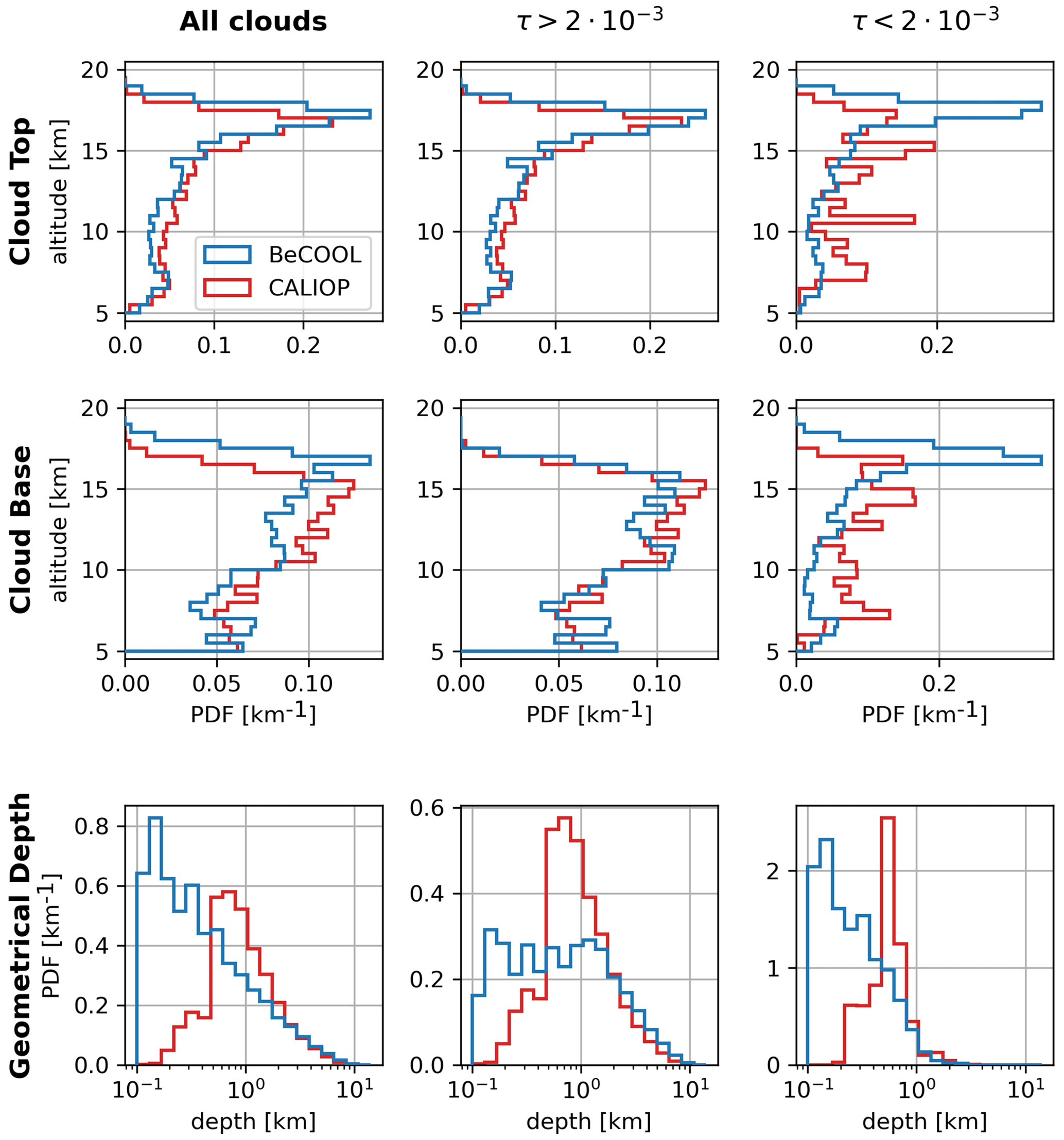
Figure 6 Statistical comparison of cloud layer properties detected by BeCOOL and CALIOP. Probability density functions of (lines) top altitude, base altitude, and geometrical depth for (columns) all clouds and clouds with an optical depth above/below the $\mathrm{2}\times {\mathrm{10}}^{-\mathrm{3}}$ threshold.

The excellent agreement between the distributions for optical depths larger than $\mathrm{2}\times {\mathrm{10}}^{-\mathrm{3}}$ shows that, despite their limited sampling, balloon-borne observations are representative of the area studied. On the contrary, for small optical depths, the comparison highlights BeCOOL's unique ability to detect ultrathin TTL cirrus. As shown in Sect. 3.2, such cirrus can persist throughout the night below the balloon and appear homogeneous. They usually lay right underneath either the cold point tropopause or a local temperature minimum, according to collocated temperature profiles from GPS–radio occultation (GPS–RO) soundings (not shown). These characteristics make those thin cirrus similar to UTTCs defined by Peter et al. (2003) and Luo et al. (2003) from the airborne measurements.

Table 5 BeCOOL mean top altitude ${\stackrel{\mathrm{‾}}{z}}_{\mathrm{top}}$ and geometrical depth $\stackrel{\mathrm{‾}}{\mathrm{\Delta }z}$ of TTL cirrus for different ranges of optical depth τ.

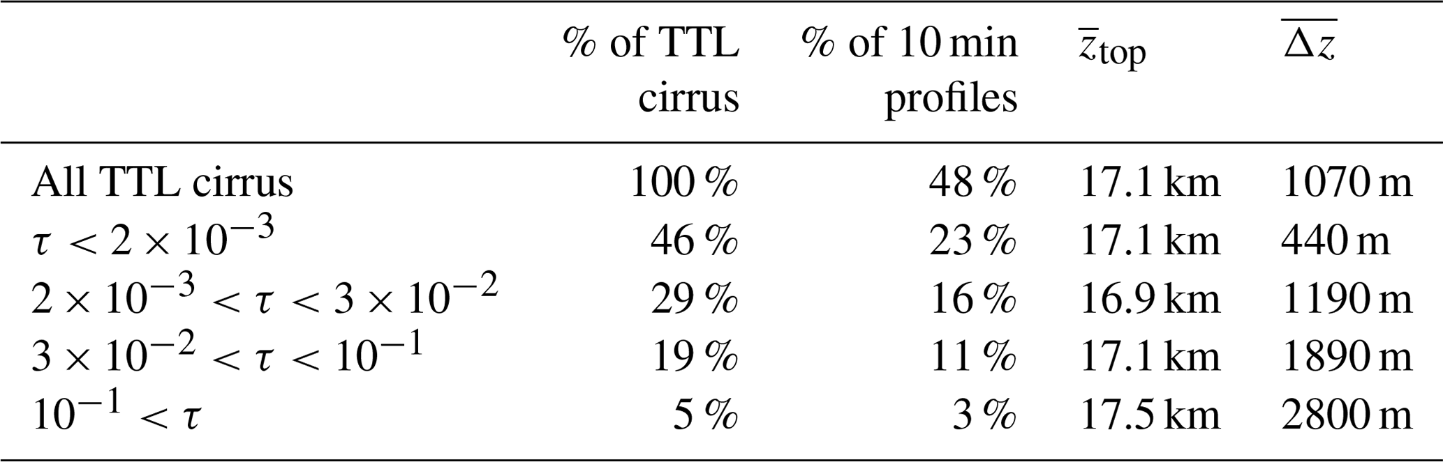
Mean top altitude ${\stackrel{\mathrm{‾}}{z}}_{\mathrm{top}}$ and geometrical depth $\stackrel{\mathrm{‾}}{\mathrm{\Delta }z}$ of TTL cirrus for different ranges of optical depth τ are summarized in Table 5. Except for the optically thicker cirrus (τ>0.1), which tend to reach higher altitudes, the mean top altitude is fairly constant. As expected, the geometrical depth is clearly correlated with τ. The depth of the cloud layer is often used as a free parameter for Lagrangian parcel box models of cirrus and stratospheric dehydration (e.g., Fueglistaler and Baker, 2006; Spichtinger and Krämer, 2013; Schoeberl et al., 2014; Poshyvailo et al., 2018; Nützel et al., 2019). Here, BeCOOL observations suggest typical depths of TTL cirrus ranging from 0.5 km (optically thinner ones) to about 3 km (optically thicker ones), with a mean of ∼ 1 km, which is overall compatible with the values used in modeling studies.

4.3 Cirrus and temperature anomalies

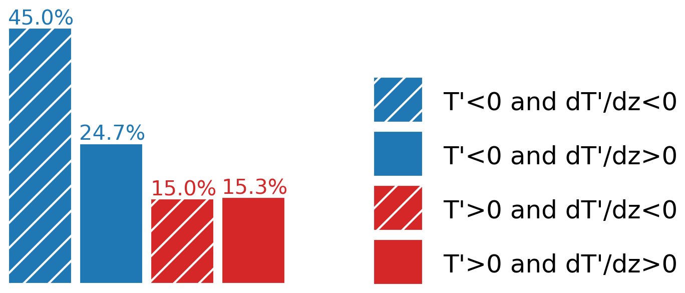
This common detection of very thin TTL cirrus layers by BeCOOL raises the question of the processes responsible for their formation. Following recent papers (Kim et al., 2016; Podglajen et al., 2018; Chang and L'Ecuyer, 2020; Bramberger et al., 2022), we investigated the relationship between TTL clouds and temperature anomalies. These previous studies highlighted the ubiquitous influence of wave-induced temperature anomalies T^′ and their vertical gradient $\mathrm{d}{T}^{\prime }/\mathrm{d}z$ on cirrus clouds. Following Chang and L'Ecuyer (2020), temperature anomalies have been computed using GPS–radio occultation (GPS–RO) temperature profiles from the Constellation Observing System for Meteorology, Ionosphere, and Climate (COSMIC) Data Analysis and Archive Center (CDAAC) of the University Corporation for Atmospheric Research (UCAR). First, for each BeCOOL flight and each night, a background temperature profile has been determined by averaging all GPS–RO profiles within a 5° latitude × 10° longitude box centered on the balloon mean position over a 14 d rolling window. Then, for each night, all GPS–RO profiles falling within a 300 km radius of the balloon and between 3 h before the first lidar observation and 3 h after the last one were selected. Finally, for each lidar observation, the corresponding temperature anomaly profile was computed as the difference between the closest GPS–RO profile in time among the selected ones and the background. We then split the cloudy lidar data points within the TTL into four categories depending on the temperature anomaly, corresponding to wave phases with positive or negative temperature anomaly T^′ and lapse-rate anomaly $\mathrm{d}{T}^{\prime }/\mathrm{d}z$. Figure 7 shows the results for the whole campaign, in a similar fashion as Fig. 3 of Chang and L'Ecuyer (2020). Our results are overall consistent with that previous study, placing almost half of the clouds in the wave phase in which both T^′ and $\mathrm{d}{T}^{\prime }/\mathrm{d}z$ are negative. As explained in Kim et al. (2016), assuming that temperature anomalies are induced by gravity waves with a downward-propagating phase, negative anomalies of $\mathrm{d}{T}^{\prime }/\mathrm{d}z$ correspond to positive vertical wind anomalies and thus to cooling conditions that lower the condensation point. Hence, our observations also suggest favorable conditions for TTL cirrus presence in the cold and cooling phase of gravity waves, which might be related to the influence of the wave-induced saturation anomalies on the formation of the ice crystals (Kim et al., 2016) and/or on their subsequent growth and sedimentation (Podglajen et al., 2018).

Figure 7 Fraction of cloudy BeCOOL lidar bins above 14.5 km within the four wave phases.

5 Conclusions

Three BeCOOL microlidars were flown during the Strateole-2 scientific campaign in the boreal winter of 2021–2022. They provide the first long-duration balloon-borne cloud lidar data set, covering the equatorial region from the Indian Ocean up to the middle of the Pacific Ocean. These observations were compared with spaceborne lidar observations from CALIOP.

Case studies of collocated BeCOOL and CALIOP observations for two different types of cirrus clouds demonstrated both the agreement between the two lidars for thicker clouds and BeCOOL's enhanced sensitivity to tenuous clouds. A longer integration time and the proximity of BeCOOL to the studied clouds are responsible for its higher sensitivity. A third case study over convective anvils illustrated the low likelihood of observing short-lived, small-scale structures, such as overshooting convective cloud tops, within a limited data set gathered from freely drifting balloons. Targeting specific uncommon cloud features would require the use of steerable balloons.

Occurrence statistics of different cloud types and profile classification reveal that cirrus clouds are ubiquitous over the area overflown by the balloons, with a wide range of optical depth covering several orders of magnitude. Cirrus clouds are detected in 73 % of the lidar profiles, with a limited regional variability during the campaign. On the contrary, the deep convective cloud cover varies very significantly between the studied regions, ranging from 15 % of the observations over the Maritime Continent to less than 1 % over the central Pacific Ocean. TTL cirrus, i.e., cirrus with a cloud base above 14 km, are found in 48 % of all profiles (and 65 % over the central Pacific Ocean). Their mean top altitude is 17 km and does not depend on their optical depth. Their geometrical depth ranges from less than 0.1 to 4 km, with an overall mean of ∼ 1 km. Ultrathin TTL cirrus, with optical depth below the detection threshold of CALIOP ($\mathit{\tau }<\mathrm{2}\times {\mathrm{10}}^{-\mathrm{3}}$), are reported in 23 % of the lidar profiles and have a mean geometrical depth of 440 m.

These very thin TTL clouds are reminiscent of ultrathin tropical tropopause clouds described by Peter et al. (2003), in particular with respect to their small vertical extension, huge horizontal extension, and lateral homogeneity. They also share these typical characteristics with laminar cirrus clouds reported notably by Winker and Trepte (1998) from LITE observations and Wang et al. (2019) from reprocessed CALIOP observations. How frequent these ultrathin cirrus are farther away from the Equator is still to be investigated, and future BeCOOL flights at higher latitudes would be useful to better characterize their coverage.

TTL cirrus clouds play a significant role in the dehydration process of air masses entering the stratosphere (e.g., Jensen et al., 1996; Schoeberl et al., 2019). An ongoing study investigates their radiative impact from BeCOOL's measurements. Our observations also confirm the ubiquitous relationship between waves and tropical cirrus clouds found in previous papers (Kim et al., 2016; Chang and L'Ecuyer, 2020; Bramberger et al., 2022): TTL cirrus are more common in the cold and cooling phase of waves. Future work will focus on characterizing the horizontal scales and lifetimes of TTL cirrus combining CALIOP and BeCOOL in order to elucidate the link between waves and the TTL cirrus lifecycle.

Appendix A: Lidar profiles at coincidence for the first case study

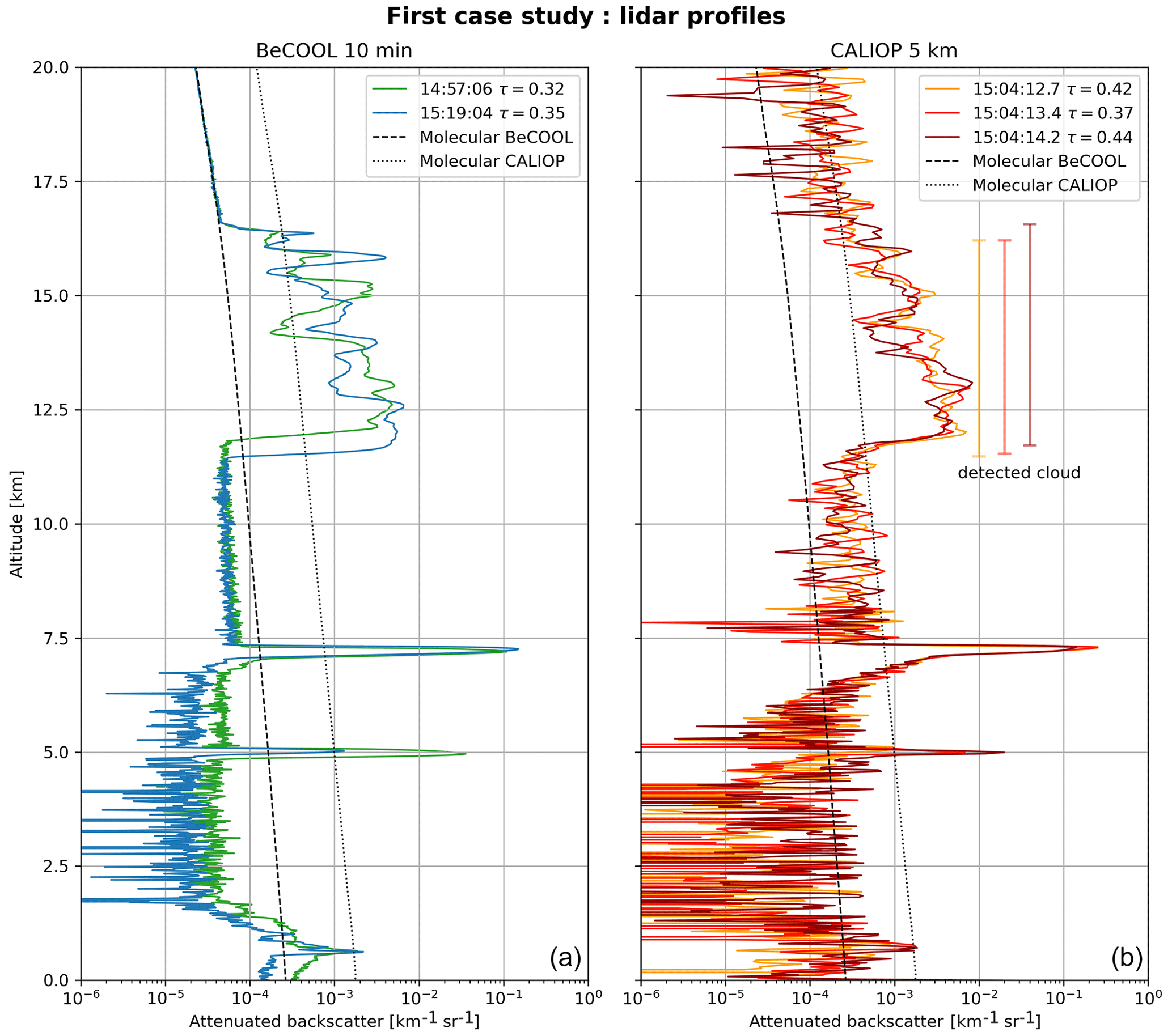
Figure A1 Attenuated backscatter profiles around coincidence for case study 1: (a) BeCOOL 10 min averaged, (b) CALIOP 5 km.

Appendix B: Additional brightness temperature maps for the case studies

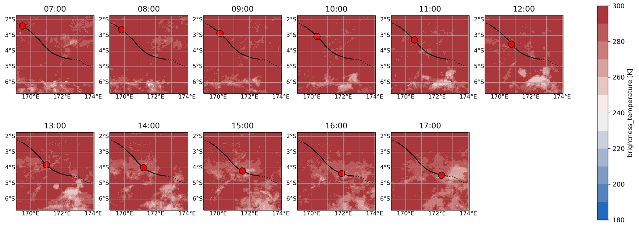
Figure B1 Hourly brightness temperature maps for case study 1, 29 November 2021. The red dot is the balloon position; the solid (dotted) line is the nighttime (daytime) balloon track.

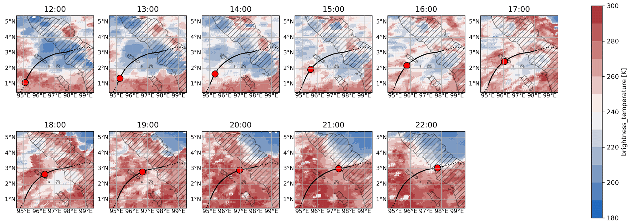
Figure B2 Hourly brightness temperature maps for case study 2, 24 November 2021. The red dot is the balloon position; the solid (dotted) line is the nighttime (daytime) balloon track.

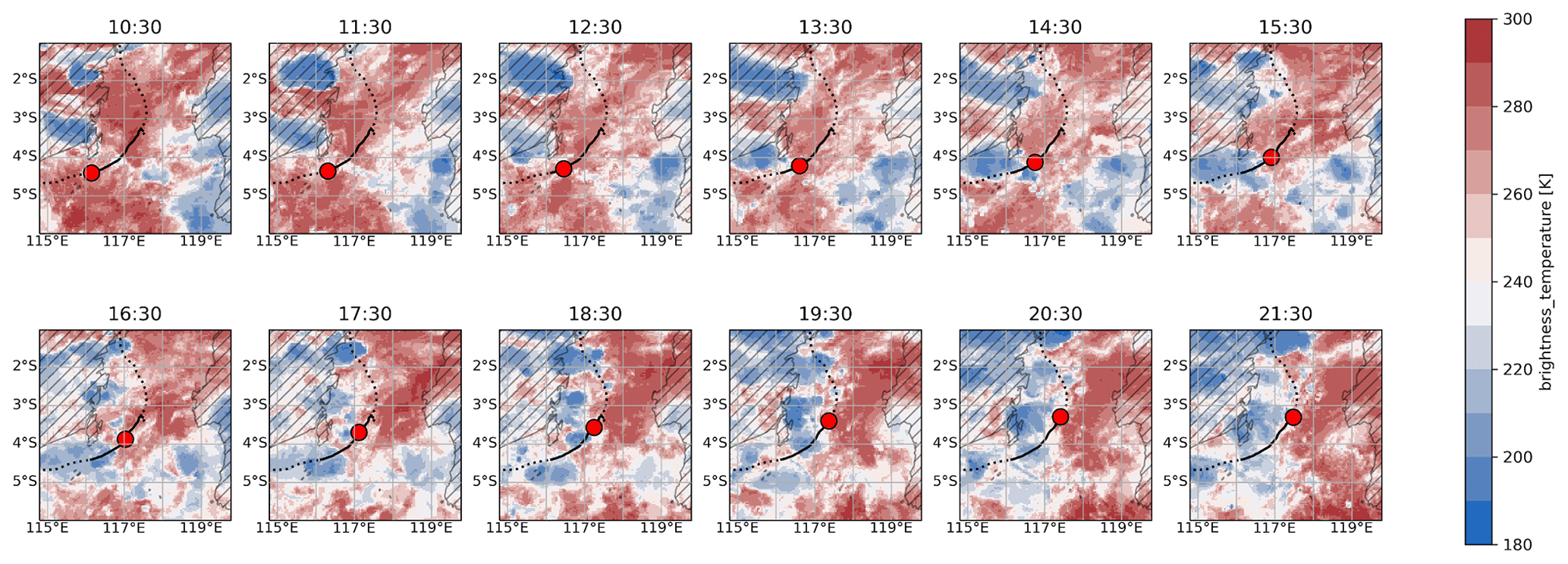
Figure B3 Hourly brightness temperature maps for case study 3, 27 November 2021​​​​​​​. The red dot is the balloon position, and the solid (dotted) line is the nighttime (daytime) balloon track.