the Creative Commons Attribution 4.0 License.
the Creative Commons Attribution 4.0 License.
 | 15 Jan 2024
Zonal variability of methane trends derived from satellite data
Jonas Hachmeister
Oliver Schneising
Michael Buchwitz
John P. Burrows
Justus Notholt
Matthias Buschmann
The Tropospheric Monitoring Instrument (TROPOMI) on board the Sentinel-5 Precursor (S5P) satellite is part of the latest generation of trace gas monitoring satellites and provides a new level of spatio-temporal information with daily global coverage, which enables the calculation of daily globally averaged CH4 concentrations. To investigate changes in atmospheric methane, the background CH4 level (i.e. the CH4 concentration without seasonal and short-term variations) has to be determined. CH4 growth rates vary in a complex manner and high-latitude zonal averages may have gaps in the time series, and thus simple fitting methods do not produce reliable results. In this paper we present an approach based on fitting an ensemble of dynamic linear models (DLMs) to TROPOMI data, from which the best model is chosen with the help of cross-validation to prevent overfitting. This method is computationally fast and is not dependent on additional inputs, allowing for fast and continuous analysis of the most recent time series data. We present results of global annual methane increases (AMIs) for the first 4.5 years of S5P/TROPOMI data, which show good agreement with AMIs from other sources. Additionally, we investigated what information can be derived from zonal bands. Due to the fast meridional mixing within hemispheres, we use zonal growth rates instead of AMIs, since they provide a higher temporal resolution. Clear differences can be observed between Northern Hemisphere and Southern Hemisphere growth rates, especially during 2019 and 2022. The growth rates show similar patterns within the hemispheres and show no short-term variations during the years, indicating that air masses within a hemisphere are well-mixed during a year. Additionally, the growth rates derived from S5P/TROPOMI data are largely consistent with growth rates derived from Copernicus Atmospheric Monitoring Service (CAMS) global-inversion-optimized (CAMS/INV) data, which use surface observations. In 2019 a reduction in growth rates can be observed for the Southern Hemisphere, while growth rates in the Northern Hemisphere stay stable or increase. During 2020 a strong increase in Southern Hemisphere growth rates can be observed, which is in accordance with recently reported increases in Southern Hemisphere wetland emissions. In 2022 the reduction in the global AMI can be attributed to decreased growth rates in the Northern Hemisphere, while growth rates in the Southern Hemisphere remain high. Investigations of fluxes from CAMS/INV data support these observations and suggest that the Northern Hemisphere decrease is mainly due to the decrease in anthropogenic fluxes, while in the Southern Hemisphere, wetland fluxes continued to rise. While the continued increase in Southern Hemisphere wetland fluxes agrees with existing studies about the causes of observed methane trends, the difference between Northern Hemisphere and Southern Hemisphere methane increases in 2022 has not been discussed before and calls for further research.
- Article
(3415 KB) - Full-text XML
- BibTeX
- EndNote


Methane (CH4) is one of the most important drivers of climate change with an effective radiative forcing of 1.19 W m−2 (Arias et al., 2021) and an atmospheric lifetime of 9.1 years (Szopa et al., 2021). The short lifespan of CH4 compared to other greenhouse gases and the large fraction of anthropogenic emissions make CH4 emission reduction an attractive strategy to slow down or possibly reduce human-made climate change in the short to medium term. Accurate knowledge of the atmospheric CH4 concentrations and dry column mixing ratios is therefore essential for improving our knowledge of the sources and sinks of CH4 for science and international environmental policy. The globally averaged surface concentration of CH4 increased by 156 % between 1750 and 2019, reaching 1866 ± 3.3 ppb in 2019 (Gulev et al., 2021) and 1917.11 ppb in June 2023 (Lan et al., 2023).
While the concentrations have risen in total, the trend, i.e. the rate of change in the background level without seasonal or short-term variations, has evolved non-linearly. Global methane concentrations have been observed to increase in the period from the 1980s to 2000 and from 2007 to the present. However, a plateau between 2000 and 2007 was observed. This is referred to as “stabilization”. Whether to define the stabilization period or the period of renewed growth (2007–present) as anomalous has been a subject of debate. There have been a variety of explanations for the observed behaviour in the literature (Turner et al., 2019). Recent publications suggest that the period of renewed growth can be attributed to the rise in microbial emissions (Lan et al., 2021; Basu et al., 2022) and the fact that tropical methane emissions explain the majority of recent changes in the atmospheric methane growth rate (Feng et al., 2022). In 2020 and 2021, record methane increases were observed by the Global Monitoring Laboratory of the National Oceanic and Atmospheric Administration (NOAA-GML) (Lan et al., 2023) and the Copernicus Climate Change Service (C3S) (c3s, 2023c). The reasons for these increases are still debated, with studies attributing them to increases in wetland emissions and changes in the atmospheric methane sink to varying degrees. The main sink of methane is through reaction with the hydroxyl radical (OH) in the troposphere. The rate of this reaction depends on the concentration of OH, which is determined by its photochemical sources and sinks. Recent studies suggest that the steep decline of nitrogen dioxide (NO2) (Cooper et al., 2022), carbon monoxide (CO), and non-methane volatile organic compound emissions as a result of the measures introduced to control and limit the spread of the COVID-19 pandemic lowered the levels of OH and thus led to part of the increase in CH4 concentrations in 2020 and 2021 (Stevenson et al., 2022; Laughner et al., 2021; Peng et al., 2022; Qu et al., 2022; Feng et al., 2023). Additionally, enhanced wetland emissions, especially from tropical wetlands, contributed to the record increases in atmospheric CH4 in 2020 and 2021 (Peng et al., 2022; Feng et al., 2023, 2022; Qu et al., 2022).
The Arctic contains large amounts of soil organic carbon (SOC), which is stored in the permafrost regions (ca. 1300 Pg), of which roughly 800 Pg is perennially frozen (Hugelius et al., 2014). The comparatively high temperature increase in the Arctic, compared to the rest of the world and also called “Arctic amplification” (Serreze and Barry, 2011; Wendisch et al., 2017), may lead to increased permafrost degradation and rapid SOC loss (Plaza et al., 2019) by the release of carbon dioxide (CO2) and/or methane. Latitudinally resolved growth rates are especially interesting in this regard and provided the initial motivation for this study.
In this paper we present methane growth rates and annual methane increases (AMIs) derived from Sentinel-5P TROPOMI XCH4 data using a dynamic linear model (DLM) approach. In the second section we present the data used. Next, we describe our method for calculating these growth rates, which is divided into four parts: (i) we discuss the preparation of the data; (ii) we provide a brief introduction to DLMs; (iii) we discuss our ensemble approach, which utilizes cross-validation to find the optimal DLM configuration for a given time series; and (iv) we provide a method to calculate a bias related to the satellite sampling. In the fourth section we present global AMIs for the first 4.5 years of Sentinel-5 Precursor (S5P) TROPOMI data and compare these to AMIs from other sources. In the fifth section we investigate zonal growth rates derived from 20∘ latitudinal bands to provide spatial information to the global AMIs. Additionally, we compare the growth rates to growth rates derived from Copernicus Atmospheric Monitoring Service (CAMS) global inversion-optimized methane data (CAMS/INV) which assimilate either surface observations or surface and satellite data. In the sixth section we investigate CAMS/INV fluxes to help with the interpretation of our previous results. Finally, we summarize our results and discuss potential future uses of this method and suggestions for further research. In the Appendix we provide additional information about our method and further results which are not included in the main text.
2.1 Sentinel-5P TROPOMI WFMD product
The S5P satellite was launched on 13 October 2017 and has since delivered high-quality data from its only scientific instrument, TROPOMI, which is a nadir-viewing passive grating imaging spectrometer. Combined with a near-polar, sun-synchronous orbit, the swath width of 2600 km provides daily global coverage. Due to the orbit geometry and swath overlap, multiple observations per day are possible in the polar regions. The spatial resolution depends on the bands and is 5.5 × 7 km2 for the short-wave infrared (SWIR) band (7 × 7 km2 before August 2019) (Ludewig, 2021). Methane is retrieved from TROPOMI measurements of sunlight reflected by the Earth's surface and atmosphere in the SWIR wavelengths. We use the latest release of the Weighting Function Modified Differential Optical Absorption Spectroscopy (WFMD) product (v1.8) (Schneising et al., 2023), which includes processing improvements such as an increased polynomial degree (cubic instead of quadratic) and an updated digital elevation model to account for various localized topography-related biases (Hachmeister et al., 2022). Furthermore, the machine-learning-based quality filter in the post-processing is improved to further reduce scenes with residual clouds. We use data with a quality flag qf=0 (good) and do not include data with qf=1 (potentially bad). The WFMD product includes measurements for solar zenith angles up to 75∘. We performed this analysis using data from May 2018 to February 2023, excluding data from the commissioning phase (November 2017 to April 2018). Uncertainties for these data are estimated during the inversion procedure via error propagation from the spectral measurement errors given in the TROPOMI Level-1 files. Additionally, the uncertainties include a correction by statistically comparing the original uncertainties to the measured scatter relative to Total Carbon Column Observing Network (TCCON) measurements.
2.2 CAMS global inversion-optimized greenhouse gas fluxes and concentrations (CAMS/INV)
The CAMS/INV dataset provides data for carbon dioxide, nitrous oxide, and methane. The methane data are produced using the CAMS CH4 flux inversion system (Segers et al., 2022), which is based on the TM5-4DVar inverse modelling system (Bergamaschi et al., 2010, 2013). We use release v22r1, where only ground-based observations from the NOAA network are used in the inversion (CAMS/INV-SRF), and release v21r1s, which includes satellite observations from the Greenhouse Gases Observing Satellite (GOSAT) in addition to ground-based observations (CAMS/INV-SRF-SAT). In our analysis we use the total column dry-air mole fractions and surface fluxes of methane from this dataset. The data are provided on a 2∘ × 3∘ grid from 1990 to 2022. We only apply our DLM approach to the methane concentrations from these data and use the corresponding fluxes directly to help with interpretation.
2.3 NOAA CH4 marine boundary layer reference
The marine boundary layer reference (MBLR) is a two-dimensional matrix (time vs. latitude) created from weekly air samples from the Cooperative Air Sampling Network (Dlugokencky et al., 2021), which is created for various long-lived trace gases by NOAA–GML. The MBLR is created by first fitting the weekly data whereby the CH4 level, seasonal component, and short-term variations are separated. For each time step (48 evenly distributed per year) the different stations give a latitudinal distribution of CH4 which is then smoothed. The global mean is calculated by averaging the smoothed latitudinal distribution for each time step. A detailed explanation can be found on the NOAA website (noa, 2023).
2.4 University of Bremen C3S/CAMS satellite data (UB–C3S–CAMS)
Annual methane increases are published by the Copernicus Climate Change Service (C3S, c3s, 2023a) in the context of the European State of the Climate (ESOTC) assessment. Here we use data from the ESOTC 2022 (c3s, 2023d) climate indicator section (c3s, 2023c). The methane data as shown on that website are (i) time series of monthly values of the column-averaged mole fraction of atmospheric methane, XCH4, as derived from satellite data; and (ii) annual mean methane growth rates including uncertainty estimates as derived from this time series.
The XCH4 time series corresponds to averaged satellite data over land in the latitude band 60∘ S–60∘ N and covers the period January 2003 to December 2022. The underlying satellite XCH4 data product for 2002–2021 is XCH4_OBS4MIPS version 4.4 available from the Copernicus Climate Data Store (CDS,c3s, 2023b) website (c3s, 2018). The data product is derived from the satellite instruments SCIAMACHY/ENVISAT, TANSO-FTS/GOSAT, and TANSO-FTS-2/GOSAT-2. A previous version of this data product is described in Reuter et al. (2020). This dataset is extended using a year 2022 satellite-derived XCH4 data product generated for CAMS (cam, 2023) (see c3s, 2023c, for details).
The combined C3S/CAMS XCH4 time series has been generated by the University of Bremen (UB) and is in the following referred to as the UB–C3S–CAMS dataset. This dataset is also used to derive annual mean methane growth rates for 2003–2022 using the method as described in Buchwitz et al. (2017) for XCO2, which was later also applied to XCH4 (Reuter et al., 2020). This method provides a new time series from the monthly XCH4 time series described above. The new time series is generated by computing the difference in XCH4 for a given calendar month between 2 consecutive years (e.g. January 2019 and 2020). The time assigned to this difference is the mean time between the 2 months (e.g. mid-July 2019). The annual mean growth rate for a given year is the weighted average of all monthly difference values of that year.
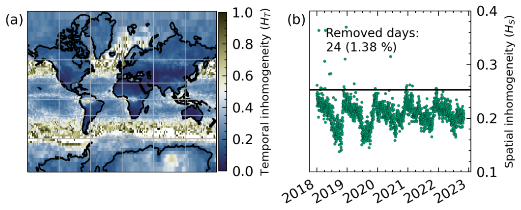
Figure 1(a) Temporal inhomogeneity (HT) for global XCH4 WFMDv1.8 data between May 2018 and February 2023. Grid cells with HT > 0.5 are omitted during analysis. (b) Spatial inhomogeneity (HS) for global XCH4 WFMDv1.8 data. Days above the HS threshold (black line) are omitted from analysis, and the threshold is set by Eq. (5), which was empirically chosen.
The Method section is split into four parts. First, we describe how the data are prepared for the DLM, meaning how we get from single observations to a time series we can fit our model to. Next, we briefly introduce DLMs and provide information on the specific types of models we are using. In the third subsection we explain how we use an ensemble of DLMs and cross-validation to select the best model. Lastly, we describe how we estimate the bias related to imperfect satellite sampling.
3.1 Data preparation
The XCH4 data to be used in the DLM fitting are pre-processed onto a latitude–longitude grid with sufficiently homogeneous sampling in space and time. Initially, the WFMD XCH4 data product is gridded onto a 2∘ × 2∘ grid. For this we assign each measurement to a single grid cell and calculate the weighted average of all measurements per cell. The measurements are weighted using the inverse measurement uncertainty to disadvantage measurements with high uncertainty. For example, reported uncertainties are higher for low-albedo scenes. Thus, these scenes contribute less to the average. The coverage of the WFMD data is roughly 25 % in all regions and is mostly constant, except for a few days with lower coverage and the seasonal data gaps at high latitudes (see Fig. D1). To account for inhomogeneities in spatial and temporal sampling, we apply the method described by Sofieva et al. (2014). This method quantifies the sampling distribution's inhomogeneity using a measure denoted as , which is defined as a linear combination of the asymmetry A and entropy E of the data.
In Eq. (2), the mean location of measurements is given by (e.g. mean spatial position or mean time), x0 is the central point, and Δx is the width of the region. Equation (3) represents the normalized entropy with N as the number of bins (e.g. grid cells or time steps), n(i) the number of observations in bin i, and n0 the sample size.
A can be intuitively understood as the asymmetry of the sampling distribution. For example, A would be high if only measurements in the Eastern Hemisphere are present for a given day. In contrast, A would be zero if the measurements are symmetrically distributed around the central point. The normalized entropy is E=1 for perfectly homogeneous sampling patterns and decreases for each missing measurement. The entropy does however not capture the distribution of the sampling pattern. Hence, a combination of both measures is used to quantify the homogeneity of the sampling distribution. Values of H close to zero indicate a homogeneous sampling distribution, while values close to one indicate a very inhomogeneous distribution. Inaccurate estimates and spurious features can arise without accounting for this inhomogeneous sampling (Sofieva et al., 2014). The inhomogeneity can be calculated in the temporal domain (for each grid cell) and in the spatial domain (for each time step).
We first calculate the temporal inhomogeneity (HT) for each grid cell, which quantifies how evenly and symmetrically the data for each grid cell are distributed in the temporal domain. HT tends to be higher in cells with sparse data coverage, which are often found over the oceans and tropical rainforests due to high cloud coverage (see Fig. 1). We then filter cells with HT>0.5. This threshold value was chosen empirically to exclude cells in these regions with limited cloud-free coverage. Next, we calculate the spatial inhomogeneity (HS) within the designated sub-grid, such as a zonal band. This allows us to identify days with very inhomogeneous coverage. The spatial inhomogeneity can be calculated along both spatial dimensions. Hence, we define HS as the equally weighted linear combination of the latitudinal and longitudinal spatial inhomogeneity:
We determine a limit, , as the median of HS plus 2 standard deviations,
and filter out days with . The equation for was empirically chosen and yields reliable limits for different sub-grids. Figure 1 illustrates the spatial and temporal inhomogeneity for global WFMDv1.8 data.
Finally, we compute the area-weighted average of the chosen sub-grid, generating a time series for the analysis. To further mitigate sampling bias in the global average, we first average over longitudes and subsequently over latitudes. This approach assumes a faster mixing of background methane levels within zonal bands while acknowledging greater latitudinal disparities. A more detailed description is given in Sect. 3.4. CAMS/INV XCH4 data are already provided on a grid with complete coverage, and no inhomogeneity treatment is necessary. The time series are therefore calculated using the area-weighted average of the sub-grid. Since the DLM approach is based on the assumption that errors are present and normally distributed, we add a Gaussian noise with σ = 0.2 ppb to the CAMS/INV XCH4 time series.
3.2 Dynamic linear model fit
To extract information about the methane growth rate from the time series we first need to calculate the underlying XCH4 level, that is the smoothly changing background concentration without seasonal or short-term variation. While a simple approach, such as fitting a polynomial plus a trigonometric function to model the seasonality, may be considered, it is insufficient due to the complex change in XCH4 levels observed in historical records (Lan et al., 2023; c3s, 2023c). The use of a moving average is not suitable due to possible data gaps, especially for high-latitude bands. Therefore, we employ dynamic linear models to fit the XCH4 data, which allow for the trend (i.e. the slope of the level, the growth rate) to change over time and can deal with missing data. For the analysis of global methane growth we use AMIs, similar to other relevant studies (Dlugokencky, 2022; c3s, 2023c; Schneising et al., 2023). This enables the methane growth of different studies to be readily compared. AMIs are defined as the difference in methane level between 1 January of 2 consecutive years. This is a measure of the integrated growth rate over the same time span. For zonal bands we directly investigate the growth rate instead of AMIs (see Sect. 5 for a more detailed description).
A dynamic linear model is a regression model that can handle observations of varying accuracy, missing data, non-uniform sampling, and non-stationary processes. It allows some of its parameters to change over time and directly models the observed variability using unobserved state variables (Laine, 2020). These DLM properties allow the analysis of not only global but also zonal methane data, which can have higher uncertainties and more gaps, especially at higher latitudes. Additionally, the direct modelling of the data allows partitioning of the signal into different components, such as an underlying level and seasonal component, which can prove advantageous beyond the scope of this paper.
A DLM can be formulated as a special case of a state-space model, i.e. a model which consists of some unobserved components (represented by a state vector) and the observation vector. The evolution of the state vector and the relation between observation and state vectors are modelled by a set of equations. If these equations are linear, we have a so-called dynamic linear model. The DLM we use consists of three main components: first, a slowly changing background level, which captures the long-term trend of the methane concentration; second, a seasonal component included to model variations arising from seasonal cycles. This component enables variations in the phase and amplitude of the seasonal cycle to be accounted for. Third, an autoregressive component is incorporated to model noise and residual correlations in the data, accounting for short-term effects. Additionally, Gaussian noise can be included to model part of the errors. The ability of DLMs to capture changing components over time is achieved by modelling these changes as Gaussian random walks, allowing for smooth transitions and adjustments. The variances of these Gaussian random walks determine the overall variability of a certain parameter (e.g. trend). A detailed description of the model set-up and the different DLM components can be found in Appendix A.
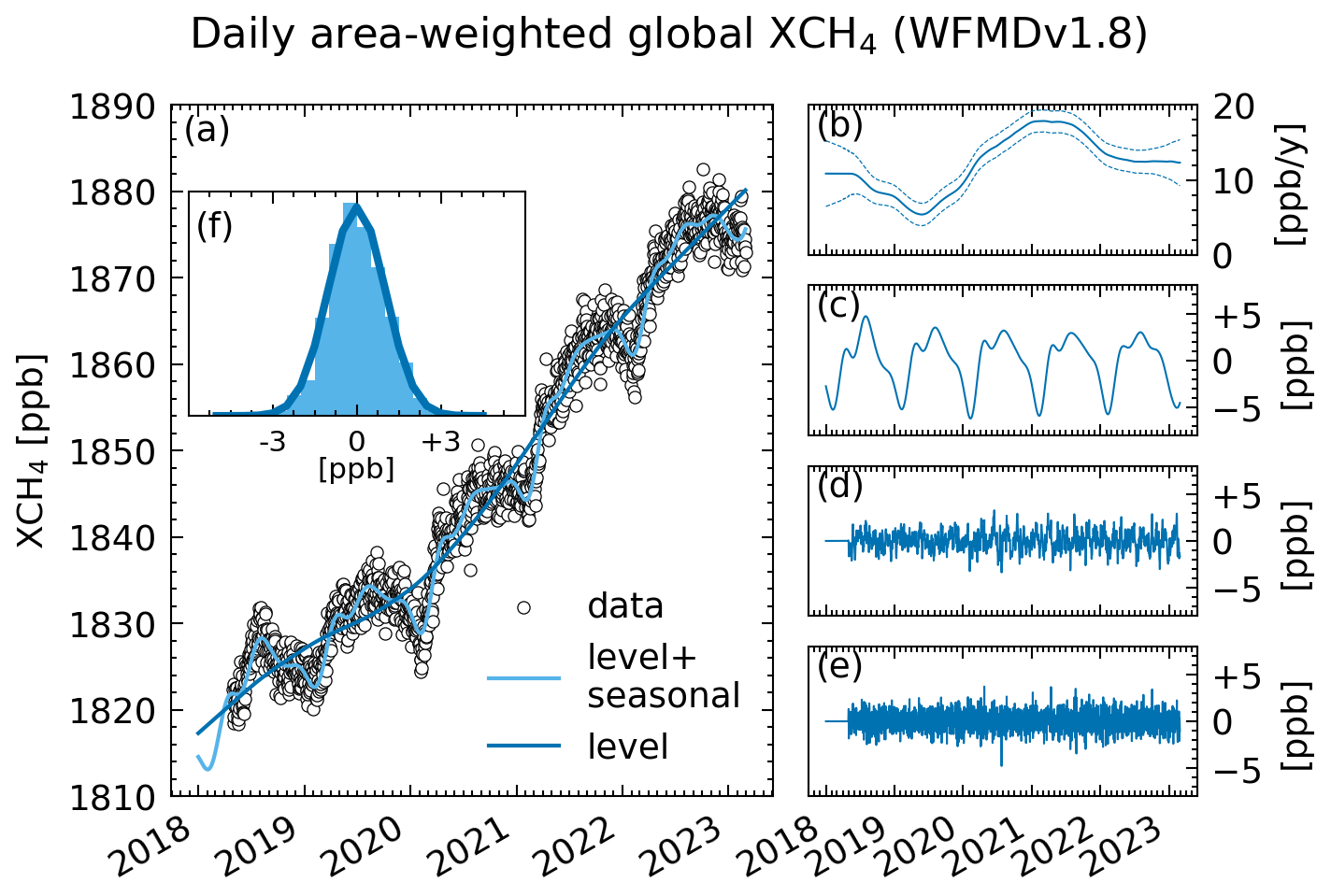
Figure 2DLM fit for daily area-weighted global WFMDv1.8 data. Panel (a) shows the daily area-weighted global XCH4 together with the level and level + seasonal components from the DLM fit. (b) The trend or growth rate is the slope of the level, the dashed lines show the 1σ uncertainty, panel (c) shows the seasonal component which captures the seasonal cycle, panel (d) shows the AR(1) component capturing residual correlations in the data, (e) the residual shows the difference between the fit and the data, and (f) a histogram of the residual shows that it is roughly normally distributed.
In general, the model parameters (e.g. variances; see Table A1 for a complete list) are not known beforehand and have to be determined. For this purpose, maximum likelihood estimation (MLE) (Durbin and Koopman, 2012; Harvey, 1990) can be used. MLE is a statistical method that estimates the parameters of a model by maximizing the likelihood of the observed data given the model's assumptions. Note that the data uncertainties are not used in the MLE but are indirectly included during the data preparation (gridding) as described above. For the end-user, various software packages exist which provide the implementation of this procedure, leaving only the model configuration open for the user. In our study we use the UnobservedComponents class of the statsmodel Python package (version 0.14.0, Perktold et al., 2023), which provides the means to define a DLM and to fit it using MLE (see sta (2023) for documentation). An overview of a DLM fit for globally averaged WFMD data can be seen in Fig. 2.
DLMs have been previously used to successfully model stratospheric ozone (Laine et al., 2014), methane from different GOSAT retrievals to investigate the seasonal cycle and trend (Kivimäki et al., 2019), and methane from ground-based remote sensing (Karppinen et al., 2020). For a detailed description of DLMs, including their formulation as a special case of a state-space model, we refer readers to Durbin and Koopman (2012) and Harvey (1990). For a more concise introduction to DLMs, we refer readers to Laine (2020).
3.3 Ensemble approach and cross-validation
The choice of model configuration is a non-trivial problem, which is impacted by prior knowledge, empirical testing, and different quality measures. From prior knowledge the inclusion of a seasonal component is inferred, because the existence of a seasonality in atmospheric methane concentrations is known. Empirical testing can show that the inclusion of an autoregressive component is necessary, because the data contain residual short-term variations. The term “quality measures” refers to measures that facilitate model selection, such as the mean squared error (MSE), which is defined as the mean of squared differences between the model and data. Additionally, the DLM provides variances (squared standard deviations) for each component which can be used to compare models; models with lower uncertainty in the level and seasonality are preferable to models with high uncertainties for these terms.
To avoid the need for manual model selection, we employ an ensemble approach, fitting a range of DLMs to the data and automatically selecting the best model. The ensemble consists of different DLM configurations, with varying components as described in Appendix A. Additionally, we perform k-fold cross-validation (CV) with k=5 folds for each DLM to calculate an average mean squared error (AMSE). During CV, the DLM is fitted on a portion of the data while leaving out another portion (the fold) for testing. The difference between the model fit and the fold is used to calculate the MSE, and the average MSE across all five folds per DLM provides the AMSE. Low AMSE values indicate a better model fit and help in selecting the best model for a given time series. The final model selection is based on an aggregated score, defined as the sum of the AMSE, the variance of the level, and the variance of the seasonal term:
The inclusion of the variances ensures that the uncertainty of the level and seasonal components is considered in the selection criterion. This approach aims to select DLMs that provide good estimates of the underlying methane signal while avoiding overfitting and reliance on expert knowledge.
Different methods and measures can be used for model selection and may yield different results. We want to emphasize that the problem of model selection is non-trivial, and different approaches may be suitable for different data and use cases. Here we select the model which yields the highest certainty fit of the level and seasonal component (i.e. the XCH4 signal without noise) while avoiding overfitting and manual selection. Furthermore, we want to mention that, in most cases, the differences between all the models in an ensemble are rather small, with the best models producing approximately the same results. However, the use of a single DLM configuration for all zonal bands is not feasible due to the inherent differences in the seasonal signal for each zonal band. Additionally, an over-specified model can lead to high uncertainties in the resulting fit.
To quantify the impact of model selection, we calculate a model selection bias , which is included in the error budget of all the AMIs and growth rates. For global data we calculate the AMIs for all the models in an ensemble and determine the weighted variance for each year of interest:
where AMIi,j is the AMI for year j and model i, AMIavg,j the average AMI of all models in year j, and σavg,j and σi,j the corresponding uncertainties as given by the DLM. For the case of growth rates we calculate a single model uncertainty which is averaged over all time steps:
where T is the total number of time steps, νi,t the growth rate for model i at time step t, νavg,t the average growth rate of all models at time step t, σavg,t the uncertainty of the average growth rate at time step t, and σi,t the uncertainty of model i at time step t as given by the DLM.
The contribution of the model selection bias to the error budget can be seen in Table 1 for global AMIs and in Table 2 for zonal growth rates. In the case of global data, the contribution is small for all years with σModel < 1 ppb except for 2018, when only an incomplete time series is available. For zonal data, σModel varies between the bands and is in the range of 1.03–4.34 ppb yr−1.
Table 1Error budget for global AMIs. σDLM is the uncertainty provided by the DLM fit, σModel is the uncertainty from model selection, and σSampling is the bias due to satellite sampling. All values show 1σ uncertainties.
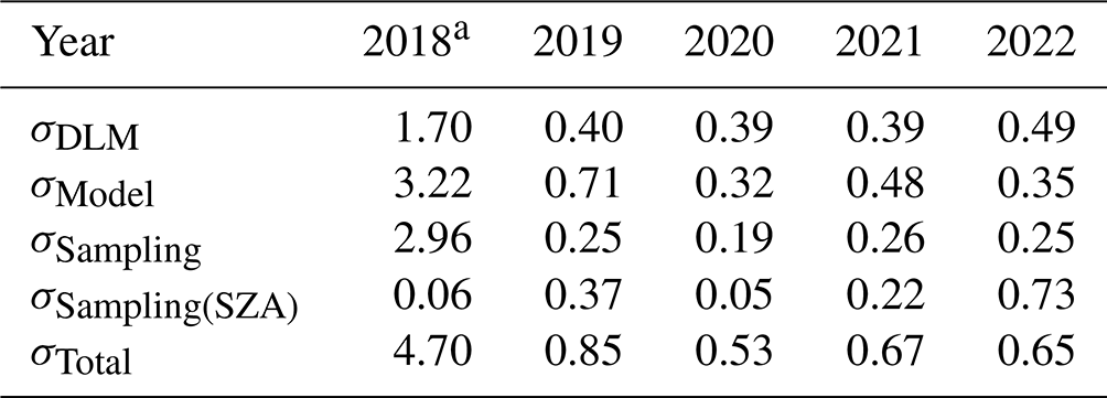
All values are in parts per billion. a 2018 only includes data starting on 1 May 2018.
Table 2Sampling and model error for zonal growth rates. σDLM is not included in this table since it varies with time but is shown in Fig. 8. All values show 1σ uncertainties.
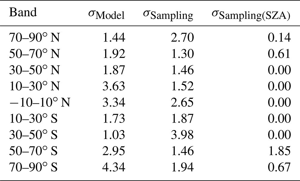
All values are given in parts per billion per year.
3.4 Estimation of sampling bias
The spatio-temporal coverage of S5P XCH4 data is limited mostly by cloud coverage, the polar nights, and poorly reflective surfaces, while additional gaps may exist due to technical problems with the satellite platform. Additionally, the sampling distribution is not completely random but is influenced by the total land mass per latitudinal band and seasonal cloud coverage over the tropical and subtropical oceans. The daily gridded data for S5P XCH4 are therefore always incomplete, meaning we have some grid cells without any measurements. Here we investigate the systematic sampling bias due to polar nights, the total effect due to sampling, and the effect of the averaging method. For this, we use CAMS/INV XCH4 data (see Sect. 2.2), onto which we apply different masks and averaging methods. Since CAMS/INV data have a complete coverage (due to being model data), we can investigate the effects of different sampling masks or averaging and compare them to the results gained from the unmasked data.
We therefore compare AMIs (for global data) and growth rates (for zonal data) calculated using different samplings and/or methods. To simulate the spatio-temporal pattern of S5P sampling, we created a daily mask from gridded WFMDv1.8 data and applied it to the model data. To only simulate the systematic effect of the polar nights, we created a daily mask using the average solar zenith angle (SZA) per grid cell with a cut-off value of 75∘. The AMIs and growth rates for CAMS/INV XCH4 data were calculated using the same ensemble approach used for WFMD data.
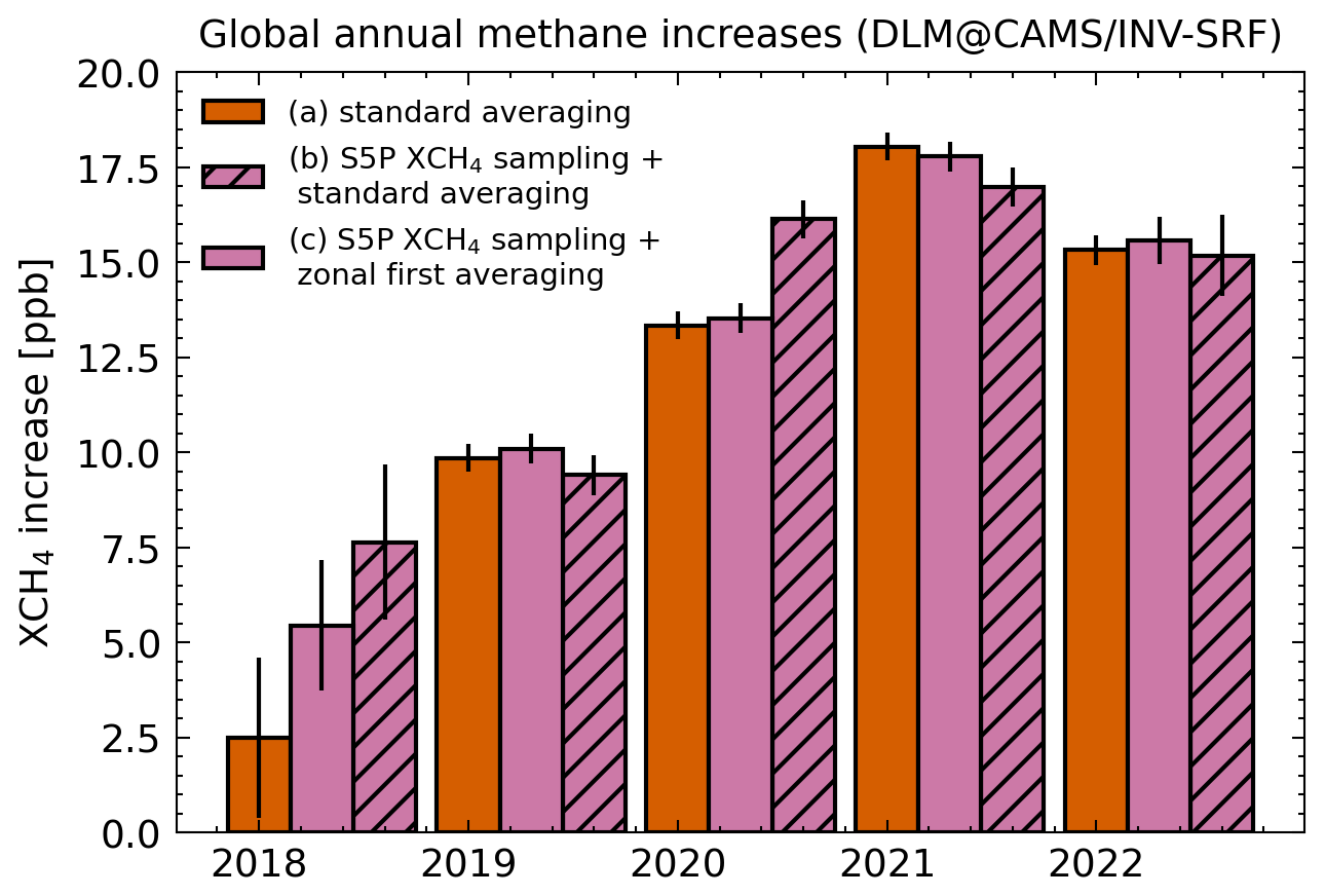
Figure 3Global AMIs derived from CAMS/INV-SRF XCH4 data using (a) the non-masked dataset with standard averaging, (b) the S5P-sampled CAMS/INV-SRF data with standard averaging, and (c) the S5P-sampled CAMS/INV-SRF data using our zonal-first averaging approach.
First, we investigate the effect of the averaging method. We compare standard averaging, which is defined in this study as the area-weighted mean of all grid cells in a region, with an approach we call zonal-first averaging. Zonal-first averaging takes into account the inhomogeneous sampling at each latitude, which is influenced by the distribution of land mass and seasonal coverage. Since zonal transport occurs within weeks (Jacob, 1999), we first average the grid cells zonally, assuming that the available data within a 2∘ band provide a good estimate of the mean XCH4 at this latitude. For global data this means that we first average the data in all 90 2∘ latitude bands, and for zonal growth rates this would mean first averaging the 10 2∘ latitude bands within a 20∘ zonal band. Subsequently, we calculate the average from the zonal averages, which leads to a consistent weighting of all the latitudes regardless of their individual coverage. Figure 3 shows AMIs calculated from CAMS/INV-SRF XCH4 data using (a) no mask and standard averaging, (b) the S5P XCH4 mask and standard averaging, and (c) the S5P XCH4 mask and zonal-first averaging. Using zonal-first averaging, the AMIs are closer to the AMIs derived from the complete data. This is especially visible for 2020, where the AMI is overestimated by roughly 3 ppb when using the standard averaging. Therefore, we use zonal-first averaging for all calculations of globally averaged data.
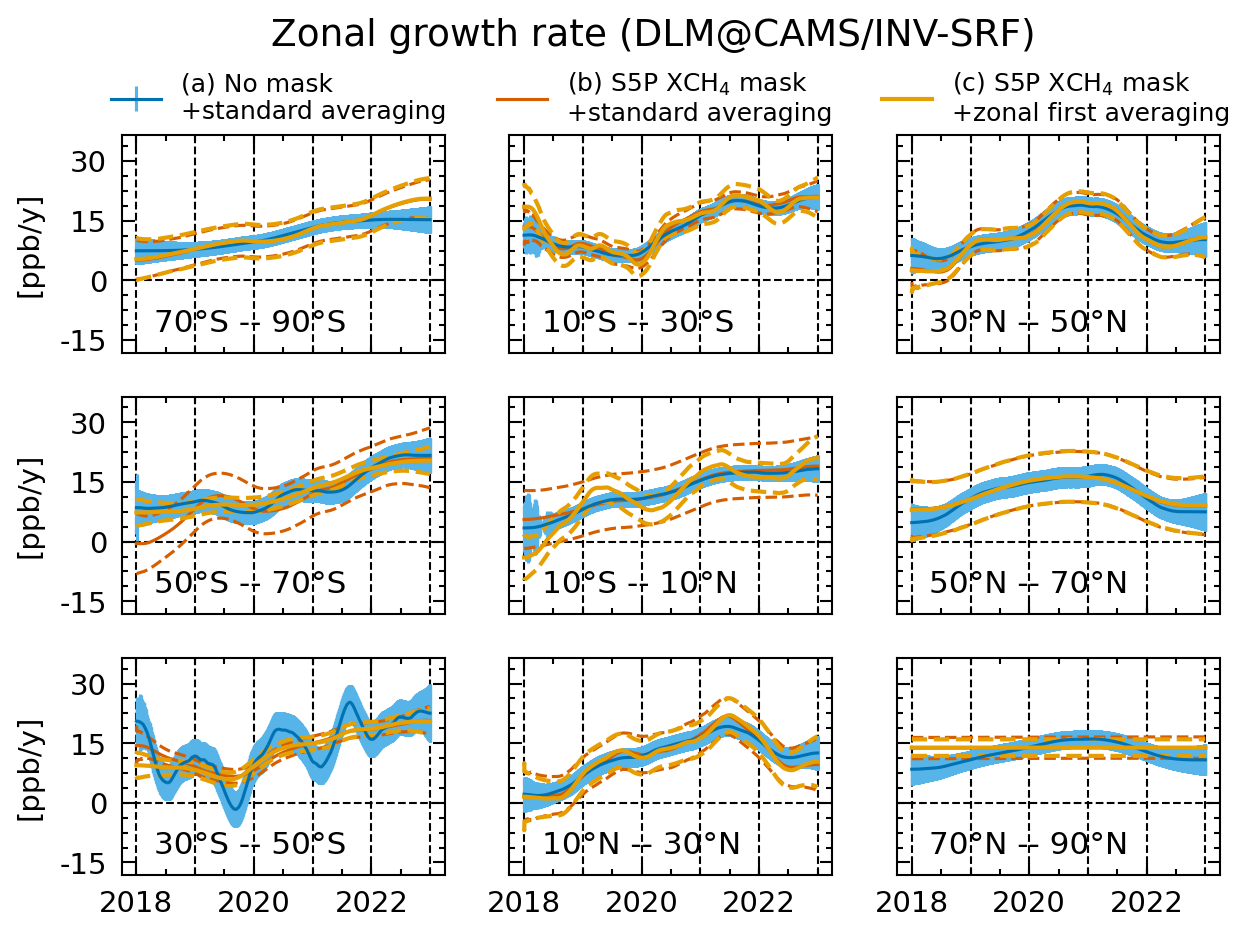
Figure 4Zonal growth rates derived from CAMS/INV-SRF XCH4 data using (a) the non-masked dataset with zonal-first averaging, (b) the S5P-sampled CAMS/INV-SRF data with standard averaging, and (c) the S5P-sampled CAMS/INV-SRF data using our zonal-first averaging approach.
Figure 4 shows zonal growth rates calculated from CAMS/INV-SRF XCH4 data using (a) no mask and standard averaging, (b) the S5P XCH4 mask and standard averaging, and (c) the S5P XCH4 mask and zonal-first averaging. Growth rates calculated on the masked data show 1σ agreement with the growth rates calculated on the complete data. Growth rates calculated using the zonal-first averaging show better agreement for the 50–70∘S band, while for the 10∘S–10∘N band the growth rate is more variable. For all the other zonal bands the results are nearly identical. Noticeably, the 70–90∘N band shows no variation when using the S5P XCH4 mask, indicating that insufficient data coverage hinders the detection of growth rate variation. Since sampling within a 20∘ zonal band can still vary with latitude, we follow the same reasoning as in the previous paragraph and also use zonal-first averaging for zonal growth rate calculation.
The different growth rates for Fig. 4a–c indicate the presence of a sampling bias. Thus, we investigated the effect of satellite sampling and the polar nights by applying corresponding masks to CAMS/INV XCH4 data. For global data the sampling biases are calculated by taking the squared difference between the AMIs calculated on the complete data (without any sampling filtering) and the AMIs calculated on the masked CAMS/INV data. We calculate a separate bias for each year in our analysis.
Table 1 shows the resulting errors for global AMIs. The sampling bias is around 0.25 ppb for all fully available years and is much higher for 2018 with 2.96 ppb. The contribution of the SZA-related bias varies from year to year with a maximum value of 0.73 ppb in the year 2022. This variability might be related to the varying difference between the high and mid latitudes during the different years. When the difference between both is bigger, the masking of high-latitude regions is expected to have a larger effect on AMIs. For the analysis of zonal bands we calculate a zonal error by taking the average squared difference between growth rates derived from the complete data and growth rates derived from the reduced CAMS/INV XCH4 data for each band:
where νi is the growth rate at time step i and N is the total number of data points. The sampling errors for zonal growth rates are shown in Table 2. Higher sampling errors correlate clearly with regions of high temporal inhomogeneity, which further shows the challenging sampling conditions in these regions (see Fig. 1).
In this section, we discuss the global AMIs calculated using WFMDv1.8 data from May 2018 to February 2023. The results are shown in Fig. 5. An overall, although non-linear, rise in the methane level is observed between 2019 and 2022. The most significant change occurs from 2019 to 2020, with an increase from 6.89 ± 0.85 ppb to 14.40 ± 0.53 ppb. The highest AMI is observed in 2021, reaching 16.93 ± 0.67 ppb. The globally averaged XCH4 rose from 1817.32 ± 2.81 ppb at the beginning of 2018 to 1878.14 ± 0.16 ppb at the end of 2022.
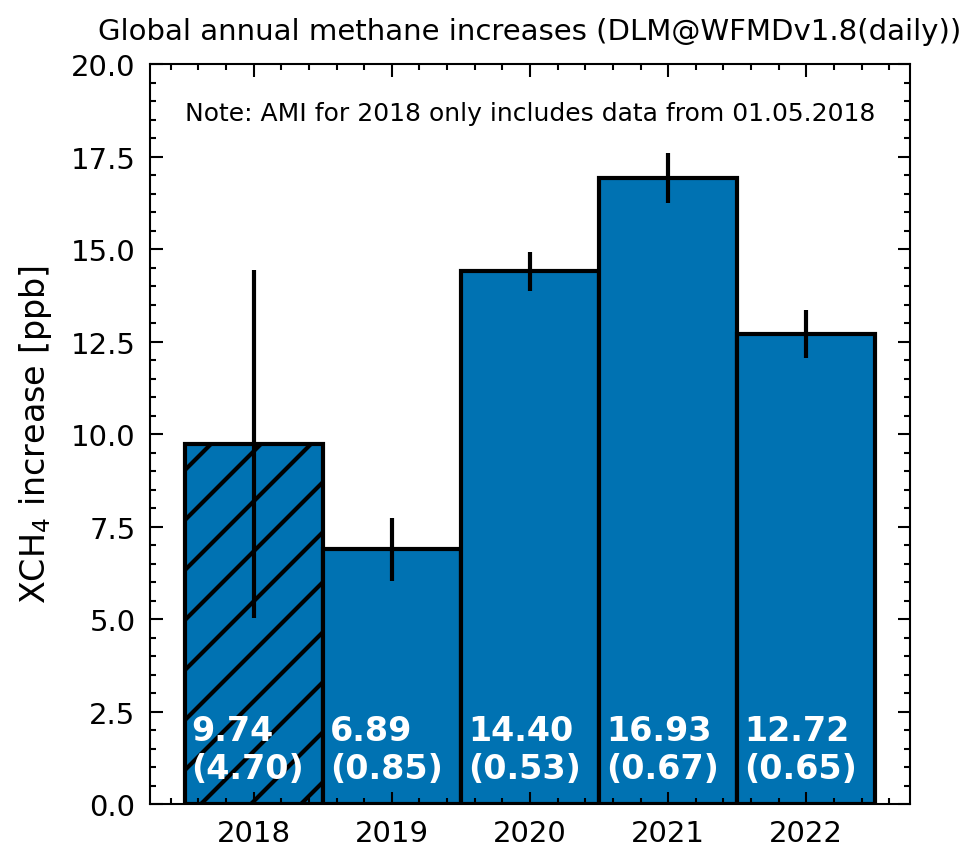
Figure 5Global annual methane increases derived from Sentinel-5P TROPOMI WFMDv1.8 data. The error bars show the 1σ uncertainty and include the DLM, sampling, and model error.
Table 3Comparison of global AMIs using different data and methods.
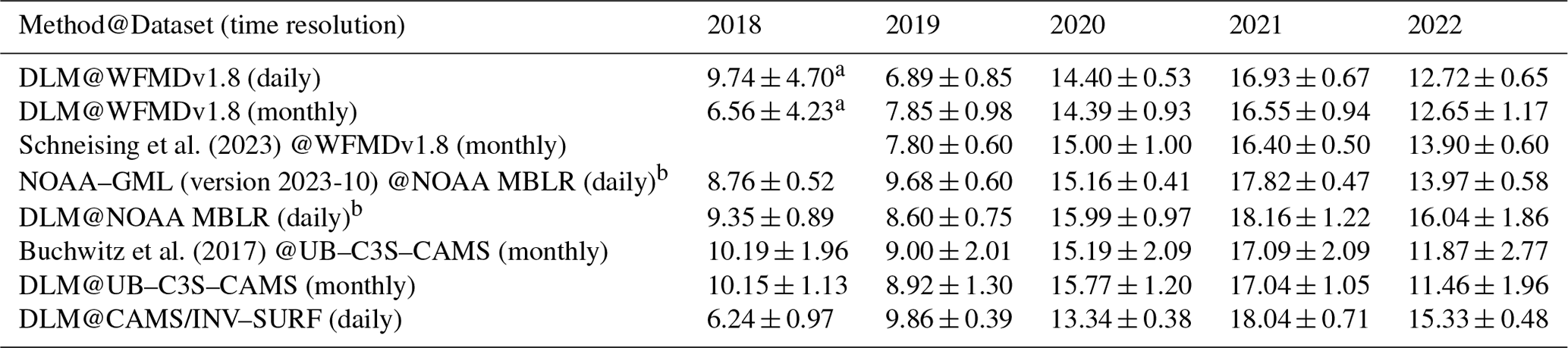
All values are in parts per billion. Uncertainties reflect 1 standard deviation. a Larger error since only data starting with May 2018 were used. b Input data have a weekly time resolution, but AMIs are provided as for daily data (as the difference between 1 January of 2 consecutive years).
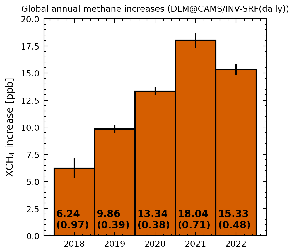
Figure 6Global annual methane increases derived from CAMS global inversion-optimized greenhouse gas concentrations including only surface observations. The error bars show the 1σ uncertainty and include the DLM and model error, which are also shown in brackets.
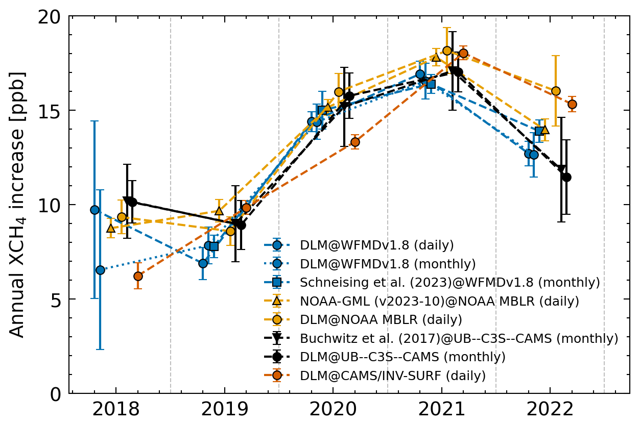
Figure 7Comparison of global AMIs listed in Table 3. The labels are formatted as Method@Dataset. Colours indicate the type of dataset used, and the markers denote the method. All errors represent 1σ uncertainties.
To validate our findings, we compared our results with AMIs determined by Schneising et al. (2023), the NOAA–GML (Dlugokencky, 2022), and data generated for the C3S (c3s, 2023c). Additionally, we include AMIs derived using our DLM approach for monthly WFMDv1.8 data, NOAA–GML MBLR data, and the UB–C3S–CAMS dataset. Table 3 and Fig. 7 provide a comparison of AMIs between 2018 and 2022. While absolute values may differ due to variations in data and methods, all the AMIs exhibit the same qualitative trend. Differences are expected for various reasons. First, there is the difference in sampling. NOAA–GML AMIs are based on surface flask measurements rather than satellite total column observations used in the other calculations. Second, different methods are used to derive AMIs from the data (see the corresponding sources for descriptions of the other methods). Lastly, depending on the time resolution of the data and the method used, the AMIs represent either the difference between 1 January of 2 consecutive years or the difference between the monthly January average of 2 consecutive years. The former is the case for our DLM approach and the AMIs derived by the NOAA–GML. The latter is the case for the AMIs derived by Schneising et al. (2023) and for the C3S AMIs. To discern the impact of data and methodology, AMIs for the UB–C3S–CAMS and NOAA–GML datasets created using different methods can be compared. Our DLM-based AMIs of these datasets agree within 1σ with the calculations done for the C3S and by the NOAA–GML, indicating no significant differences due to the method used. However, we see a comparatively high AMI in 2022 for the combination of DLM and NOAA–GML data (see Fig. 7). This is probably related to the higher uncertainty for DLMs at the start and end of a time series, which can also be seen for UB–C3S-CAMS AMIs. A longer input time series will likely lead to a reduction in uncertainty and to a reduced deviation compared to the other 2022 AMIs. An application of our DLM approach for the complete UB–C3S–CAMS and NOAA–GML MBLR data can be seen in Appendix B.
Additionally, we used our DLM approach on monthly WFMDv1.8 data to better compare our method to the method used by Schneising et al. (2023), which also shows agreement within 1σ. Only differences smaller than 1σ are found when comparing AMIs based on the same data but different methods. We also applied our approach to CAMS/INV XCH4 data (see Sect. 2.2), for which global AMIs can be seen in Fig. 6. The AMIs are in qualitative agreement and show the same structure over the 5-year period; however, significant differences in absolute values are observed for 2020 and 2022. For 2020 the CAMS/INV AMI is significantly lower compared to most other sources, while for 2022 the CAMS/INV AMI is significantly higher compared to most other sources (see Table 3).
The AMIs for 2020 and 2021 are the largest observed since the NOAA began systematic records in 1983. The drivers contributing to these record increases have been the subject of recent debate and can be attributed to a rise in emissions, a reduction in the CH4 sink, or a combination of both effects. According to the International Energy Agency (IEA), methane emissions from the energy sector decreased by approximately 10 % in 2020 (iea, 2021). However, additional emissions due to reduced maintenance of landfills and oil and gas infrastructure can be expected according to Laughner et al. (2021), while McNorton et al. (2022) suggest that the effect of the global slowdown on anthropogenic CH4 emissions is relatively small. Some studies propose that the reduction in the OH sink, caused by decreased emissions of nitrogen oxides during the COVID-19 pandemic, may explain part of the increase (Stevenson et al., 2022; Laughner et al., 2021; Peng et al., 2022; Qu et al., 2022; Feng et al., 2023). Specifically, Stevenson et al. (2022) and Peng et al. (2022) suggest that approximately half of the increase can be attributed to this effect. Conversely, several other studies attribute the majority of the CH4 increase in 2020 to the growth in wetland emissions (Qu et al., 2022; Feng et al., 2023, 2022; Zhang et al., 2023).
In addition to our global analysis, we investigated 20∘ zonal bands. The good spatio-temporal coverage of S5P XCH4 might suggest that the same approach of using AMIs could be applied to identify zonal bands with anomalous methane increases. However, the impact of atmospheric transport has to be considered. While longitudinal mixing occurs on timescales of a few weeks, meridional transport is slower, taking 1–2 months between mid-latitudes and the tropics or polar regions and around a year between hemispheres (Jacob, 1999; Warneck, 1999). The relatively longer atmospheric lifetime of 9.1 years (Szopa et al., 2021) compared to the mixing times therefore guarantees a relatively even latitudinal distribution of methane in the troposphere, where the main difference is driven by the uneven distribution of CH4 sources (Warneck, 1999). Thus, we need to sample at about 1 year or less to observe differences between hemispheres and 1 month or less to observe differences within a hemisphere. The daily sampling of S5P is hence faster than meridional transport; however, part of the temporal information gets lost when using AMIs which are obtained by integrating the growth rate over 1 year. Thus, we investigate the growth rate, which is the trend component of our DLM fits, to obtain a better temporal resolution of the zonal signals.
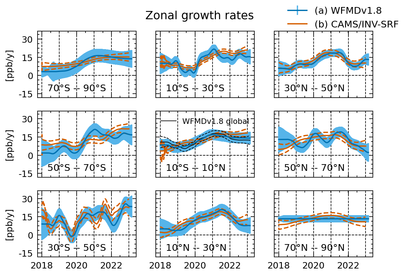
Figure 8Zonal growth rates for 20∘ bands derived from (a) Sentinel-5P TROPOMI WFMDv1.8 data and (b) CAMS/INV-SRF XCH4 data. The errors show the 1σ uncertainty.
The results are shown in Fig. 8 and include growth rates derived from CAMS/INV-SRF XCH4 data for comparison. The shown errors include the uncertainty gained from the DLM fit σDLM, the model selection error σModel, and the sampling error σSampling (see Sects. 3.3 and 3.4). Growth rates are similar within a hemisphere, while differences between the hemispheres are clearly visible. Additionally, no significant sub-annual variations (i.e. on a monthly timescale) in zonal growth rates are present. Both observations are in good agreement with the known atmospheric mixing times and indicate that our data currently allow for identification of inter-hemispheric differences, while short-term variations between zonal bands are not detected. The high-latitude band between 70 and 90∘ N is included for completeness but shows no inter-annual variability. This may be due to a lack of real change in growth rates in this region, high uncertainties present in the data, and/or the sparse data coverage. The corresponding CAMS/INV-SRF XCH4 growth rate indicates that the variability in the growth rate is relatively small in this band, which supports the first point of our explanation. We therefore exclude this band from our following discussion. Hence, we mean bands between 10 and 90∘ S when we speak of the Southern Hemisphere (SH) and bands between 10 and 70∘ N when we speak of the Northern Hemisphere (NH). The band between 10∘ S and 10∘ N represents the boundary region and is close to the global background, as can be seen in Fig. 9, which presents zonal growth rate anomalies. Zonal growth rate anomalies are defined as the difference between the zonal and global growth rates for each band.
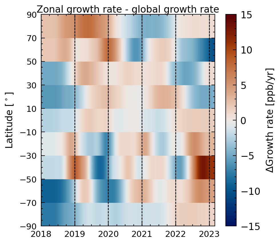
Figure 9Zonal growth rate anomalies for the 20∘ bands derived from Sentinel-5P TROPOMI WFMDv1.8 data. The anomalies are defined as the differences between zonal and global growth rates.
Overall growth rates derived from WFMD data are close to growth rates derived from CAMS/INV-SRF XCH4 data, with an overall agreement within 1σ. The growth rates and the growth rate anomalies can be used to interpret the changes in global AMIs and to allow the identification of hemispheres or zonal bands with anomalous growth rates. Differences between the hemispheres can be especially well seen in the zonal growth rate anomalies. During 2019 a decrease in growth rates can be observed for the whole SH (except for the southernmost band), while growth rates in the NH increased or stayed stable. For 2020 growth rates for all the SH bands increase greatly from roughly 0 to 20 ppb yr−1. The NH growth rates increase more slowly, except for the 50–70∘ N band, which exhibits a small decrease in the growth rate. During 2021 most zonal growth rates move towards or around the global mean, with the strongest anomaly visible in the 10–30∘ N band, which shows some additional increase in the growth rate that peaks in the middle of the year. During 2022 a clear difference between the hemispheres can be seen again, with a decrease in growth rates in the NH and an increase in or stabilization of growth rates in the SH. This difference is especially clear when looking at the zonal growth rate anomalies in Fig. 9.
Recent studies, which discuss the record methane increases in 2020 and 2021, can help with interpreting the structures of zonal growth rates. Peng et al. (2022) employ an atmospheric inversion using ground-based data. They attribute the increase from 2019 to 2020 roughly equally to changes in the OH sink and an increase in wetland emissions located mainly in the NH. In contrast, studies based on the inversion of satellite data from the Japanese Greenhouse gases Observing SATellite (GOSAT) state that the majority of increase from 2019 to 2020 can be attributed to the African continent (Feng et al., 2023; Qu et al., 2022) with additional increases in tropical South America in 2021 (Feng et al., 2023). Our findings can thus be seen as aligning with recent studies by Feng et al. (2023) and Qu et al. (2022). The increase in SH growth rates from 2019 to 2020 is consistent with increased wetland emissions. The rise in the NH latitudinal bands during 2020 can be explained by the decreasing OH sink primarily located in the NH (Peng et al., 2022; Feng et al., 2023). However, the continued increase in 2021 cannot be solely explained by the OH sink, as OH levels mostly recovered in that year according to Feng et al. (2023) and Peng et al. (2022). Possible explanations for the ongoing increase are persistent wetland emissions Feng et al. (2023) as well as the return to pre-pandemic methane emissions form the energy sector in 2021 (iea, 2023). Finally, the decrease in growth rates in the NH and the increase in growth rates in the SH during 2022 have not been discussed to our knowledge. Our results therefore indicate that the decrease in global AMI from 2021 to 2022 can be attributed to a reduced growth rate in the NH. We investigate this further in the next section.
As mentioned before, zonal growth rates provide information about the change in methane concentration in a given zonal band, including changes in sources, sinks and transport patterns. These transport patterns would average out for global AMIs given a perfect coverage. In Sect. 3.4 we applied a S5P XCH4 mask to CAMS/INV XCH4 data (see Fig. 3) and compared AMIs calculated from this masked data with AMIs calculated from the complete data. Since differences between these AMIs are small, we conclude that the effect of related sampling biases is limited. Therefore, changes in global AMIs can be attributed to the total source–sink balance of methane and not to changes in transport patterns. Whether this is also true for zonal growth rates is less clear, since transport effects are expected to be stronger especially within hemispheres.
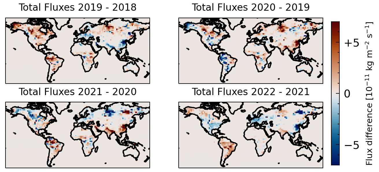
Figure 10Difference between total surface fluxes from the CAMS/INV-SRF data.
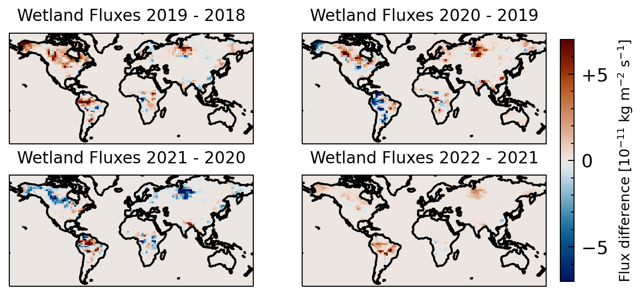
Figure 11Difference between wetland surface fluxes from the CAMS/INV-SRF data.
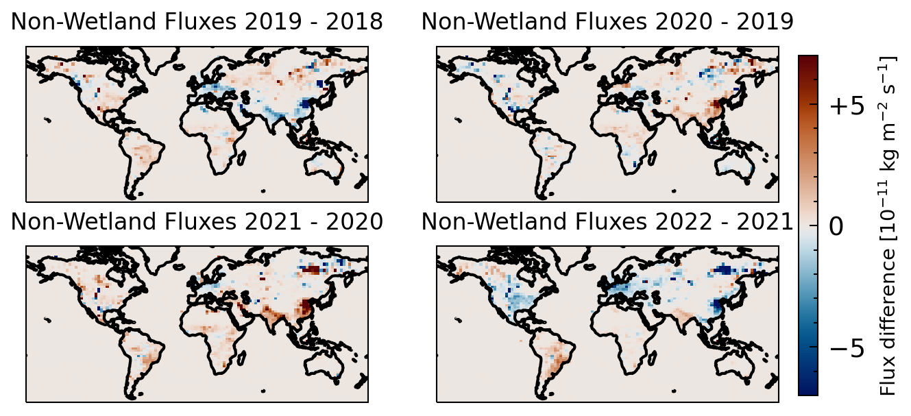
Figure 12Difference between other surface fluxes from the CAMS/INV-SRF data.
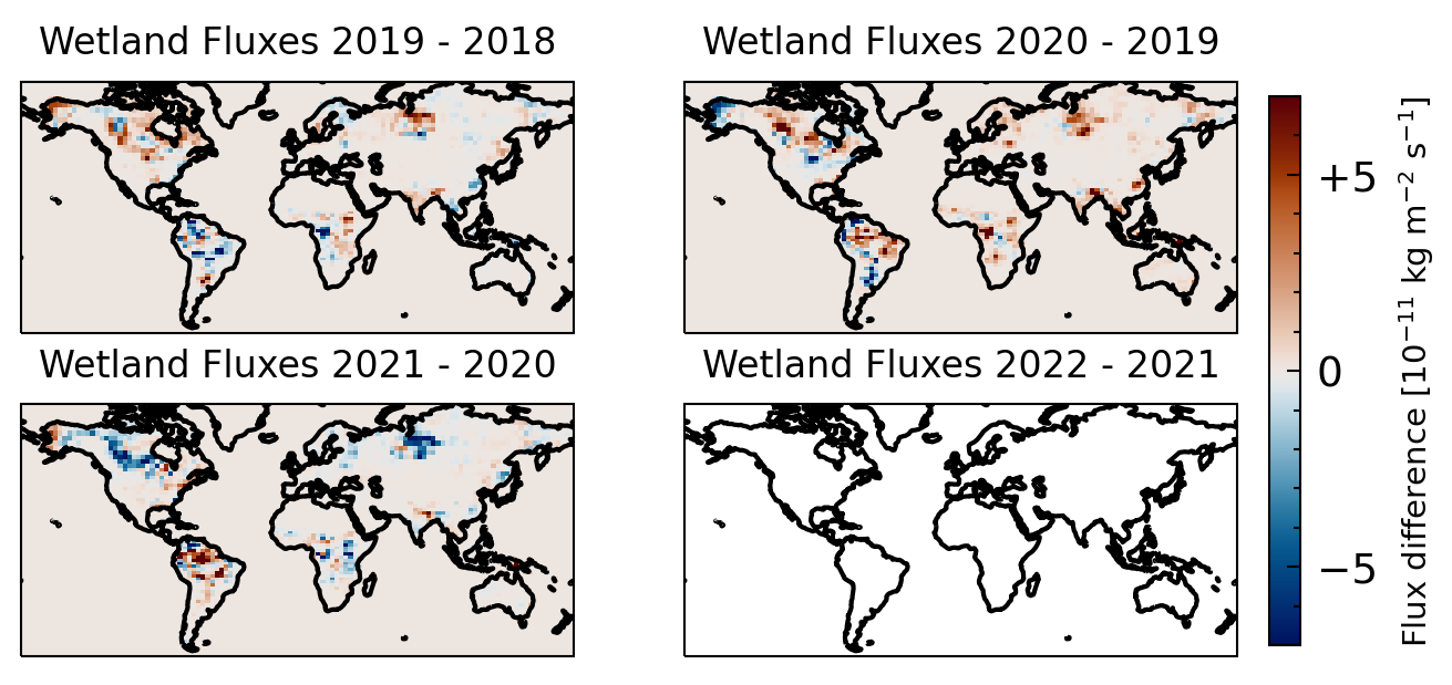
Figure 13Difference between total surface fluxes from the CAMS/INV-SRF-SAT data. No flux difference is available for 2022–2021, since the dataset currently ends in 2021.
The agreement within 1σ of zonal growth rates derived from WFMD and CAMS/INV XCH4 data in Fig. 8, suggest that the structures observed in our zonal growth rates are not artifacts from sampling-related biases. However, we cannot rule out transport effects from this comparison, meaning we cannot clearly attribute changes in hemispheres or zonal bands over the years to a change in the source–sink balance. Hence, we also investigated the change in surface fluxes between consecutive years which are readily available for the CAMS/INV data. In Figs. 10–12 we present total, wetland and non-wetland fluxes from CAMS/INV-SRF data, respectively. The category of non-wetland fluxes includes all other anthropogenic emissions as well as contributions from oceans, wild animals, the soil sink, termites, and biomass burning.
Large changes in fluxes are identified between all the years investigated. The wetland flux difference between 2019 and 2020 indicate a strong increase in the NH as indicated by Peng et al. (2022) as well as some increase in the SH wetlands as reported by Feng et al. (2023) and Qu et al. (2022). We expect the SH wetland fluxes to be underestimated as indicated by Feng et al. (2023) because the CAMS/INV-SRF data is based on ground-based measurements from the NOAA network, similar to the inversion performed by Peng et al. (2022), due to the poor coverage in the tropics. Interestingly, wetland fluxes from CAMS/INV-SRF-SAT data including satellite measurements from GOSAT show stronger SH wetland emissions between 2019 and 2020 as shown in Fig. 13. Additionally, an increase in non-wetland fluxes occurs between 2019–2020 and 2020–2021. In the first case these increases are mainly focused on China, while in the second case additional increases over the Indian subcontinent can be seen. Between 2021 and 2022 a clear decrease in total surface fluxes can be seen in large parts of the NH, while strong increases can be observed over the whole of South America. The large decreases in the NH can be clearly attributed to changes in the non-wetland fluxes, while the increase over South America seems to involve a combination of wetland and other fluxes. Therefore, CAMS/INV fluxes imply that the changes in zonal growth rates we observed both in WFMD and CAMS/INV are not merely due to changes in transport patterns but correlate with changes in surface methane fluxes between the years. This conclusion is strengthened by the qualitative agreement of the flux changes between CAMS/INV-SRF and the aforementioned studies by Peng et al. (2022), Feng et al. (2023), and Qu et al. (2022). However, further research is needed to substantiate these inferences.
In this study, we presented a DLM-based approach to calculate methane growth rates and AMIs from S5P/TROPOMI data. We addressed sampling-related biases by comparing AMIs and growth rates derived from CAMS/INV XCH4 data both with and without S5P XCH4 sampling. Further, we included a bias related to the model selection in our error budget. Our calculations of global AMIs based on WFMDv1.8 data from 2018 to 2022 demonstrate good agreement with other AMIs. Additionally, we separated the influence of the fitting method and the underlying data by applying our DLM approach to other datasets. We show that using the same input data results in agreement within 1σ between all AMIs. Using the same method but different input data results in qualitative agreement but differences larger than 1σ. Nevertheless, the consistency of AMIs derived from diverse datasets, such as ground-based data from NOAA and dry-air mole fraction data from WFMDv1.8 and UB–C3S–CAMS, highlights the robustness of these various approaches. The record methane increase in 2020 and 2021 is therefore well-identified in the different datasets, which use different methods to assess AMIs. The underlying factors driving these increases, as discussed in Sect. 4, remain however a subject of debate.
In addition to global AMIs, we investigated growth rates for 20∘ zonal bands which provide spatial information to the global AMIs. We argue that this is possible due to (a) the faster zonal mixing in comparison to meridional mixing and (b) the faster satellite sampling in comparison to the meridional mixing times. Firstly, comparisons of zonal growth rates from S5P/TROPOMI data with growth rates from CAMS/INV-SRF XCH4 data show agreement within 1σ. Additionally, we investigated growth rates calculated from CAMS/INV-SRF XCH4 data filtered using a S5P XCH4 mask which indicate that no significant sampling biases exist for the zonal band approach. Still, we want to emphasize that meridional transport can affect the zonal growth rates, meaning they do not necessarily indicate changes in the sources and sinks of methane but might also show systematic changes in transport patterns. The zonal growth rates exhibit clear differences between the hemispheres for 2019 and 2022, whereas growth rates are more similar for 2020 and 2021. Differences within a hemisphere are mostly smaller and no additional short-term variations are visible, which might reflect the well-mixed state of the atmosphere within a hemisphere. The low growth rates in the SH in 2019 and the subsequent increases suggest a rise in atmospheric methane in that region possibly driven by tropical wetland emissions according to Feng et al. (2023), Qu et al. (2022), and Zhang et al. (2023). Other factors potentially contributing to these changes include variations in the OH sink due to pollutant reductions during the COVID-19 pandemic (Feng et al., 2023; Qu et al., 2022; Peng et al., 2022) and the changes in global methane emissions due to the COVID-19 pandemic and the subsequent recovery (iea, 2021).
We further investigated these inter-hemispheric differences by investigating the surface fluxes available from CAMS/INV data. We argue that this is possible since (a) growth rates derived from WFMDv1.8 data are similar to growth rates from CAMS/INV data and (b) no significant sampling bias is present, as we showed in Sect. 3.4. The total surface fluxes show clear changes between the years, and the partitioning into wetland and non-wetland (mainly anthropogenic) fluxes allows further interpretation. Furthermore, changes in fluxes show reasonable qualitative agreement with findings reported by Feng et al. (2023), Qu et al. (2022), and Peng et al. (2022).
In addition to the confirmation of known results, new conclusions are also drawn. Most notably, the decrease in the global AMI in 2022 is caused by reduced NH zonal growth rates. This is clearly visible in zonal growth rates derived from S5P XCH4 and CAMS/INV XCH4 data. Investigation of the corresponding model surface fluxes indicates that changes in zonal growth rates are consistent with the decrease in non-wetland fluxes in the NH and the continuing increase in wetland fluxes in the SH. However, more research is needed to substantiate this inferred connection between the change in NH growth rates and fluxes.
In summary, our DLM-based approach allows calculation of growth rates or AMIs for global and zonal S5P/TROPOMI data. This approach is computationally inexpensive and readily allows for the constant integration of new data, enabling timely assessments of global methane concentration changes. Importantly, no additional prior information about the atmospheric state is required. We believe that our approach provides an additional valuable tool for investigating atmospheric methane concentrations, enabling rapid identification of regions of interest, such as the 2022 NH. Furthermore, our approach can be readily applied to other datasets facing similar challenges, such as inhomogeneous sampling, non-linear trends, and data gaps. For the 70–90∘ N band, our method failed to identify any changes in growth rates. However, this result is in good agreement with the growth rates from CAMS/INV-SRF XCH4 data, which themselves only show small variations. This indicates that (a) the small changes in growth rates could not be distinguished from the random variability in the data or that (b) no anomalous increases in growth rates are visible for the northern high-latitude regions in the observed period from 2018 to 2022.
Future research could aim to improve this approach, especially for high-latitude regions, to identify smaller changes in growth rates. Better estimates of the impact of meridional transport on zonal growth rates could help to provide better error estimates for our method. The 2022 decrease in NH growth rates could be investigated in more detail and this approach be extended to include datasets of other atmospheric constituents. Data from future satellite missions, with lower uncertainties and increased data coverage, could enable the investigation of sub-annual changes in growth rates, which are presently not detectable. Finally, zonal growth rates of long-lived gases (e.g. HF) without any significant sources or sinks could possibly enable the quantification of atmospheric transport patterns.
The structure of our DLMs assumes that the measured methane signal can be separated into a slowly changing background level, a seasonal component and noise term. This section closely follows the more detailed description in Durbin and Koopman (2012) and Harvey (1990).
The level component can be described by the following formulas:
μt is the level, νt is the trend (i.e. the slope or growth rate), and ϵt are steps in a random walk sampled from a Gaussian distribution. The random walks allow components to change over time. Since we want to allow for a smoothly changing level, we allow the trend to change over time. Additionally, we enforce a constraint of zero variance for the level to ensure that short-term fluctuations in the background level are not allowed:
The seasonal part of the signal is modelled by a truncated Fourier series with h harmonics:
with
where s describes the seasonality of the data, e.g. for monthly data s=12 or for daily data s=365 when modelling yearly patterns. The value of s=365.25 can be used to account for leap years. We use s=365.2, which is equal to the average number of days per year between 2018 and 2022. For the seasonal cycle is allowed to change over time. We allow values of to account for varying levels of complexity in the seasonal cycle. The motivation for this is twofold. Firstly, we want to only model the basic structure of the seasonal cycle and not the whole signal. Secondly, the inclusion of more harmonics introduces further parameters which have to be estimated. This quickly leads to high uncertainties in the produced fit since not enough information is included in the data to account for the growing number of parameters.
Table A1DLM parameters.
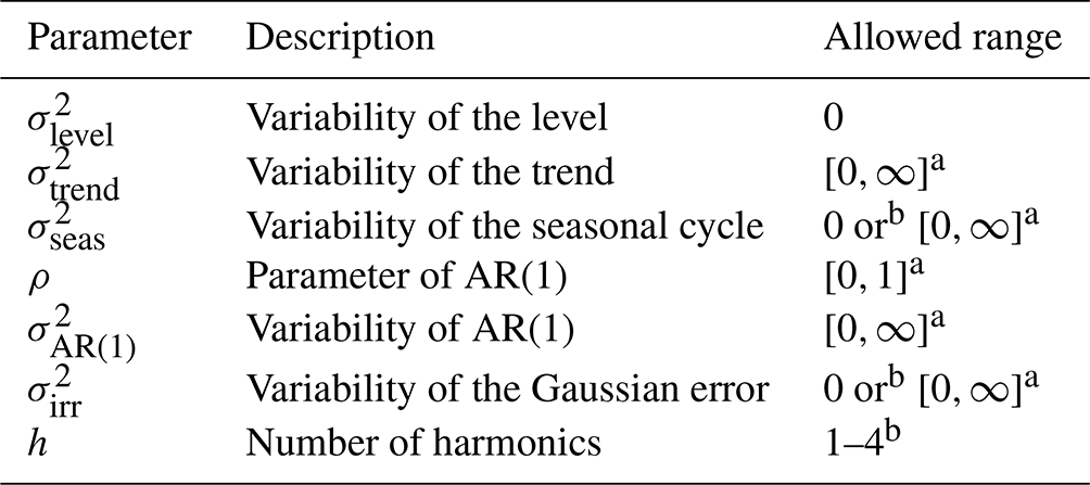
a Determined by maximum likelihood estimation during the DLM fit. b Different settings are part of the ensemble.
The noise term accounts for residual correlations as well as random Gaussian noise in the signal. Residual correlations can be modelled by an autoregressive component which includes a serial dependence between the observations. An autoregressive noise of order n includes a memory of the last n measurements. For n=1, this AR(1) term is
where ηt is the autoregressive component, ρ determines the strength of the autocorrelation (the memory of the previous time step), and ϵAR(1) is again a step in a Gaussian random walk. This component introduces the parameters ρ and to the model. We confine our autoregressive component to the order of n=1, which is enough to model the residual correlations in our data. Higher orders would introduce further parameters to be estimated and lead to a harder interpretability of the results. However, exclusion of the AR(1) component leads to bad fits since the model fails to account for the data variability.
An additional Gaussian noise can be included:
We call this the irregular component.
The complete signal can then be written as the sum of these components:
The ensemble size is determined by the number of possible model configurations. In our case this is determined by whether to allow variability of the seasonal cycle or whether to include a Gaussian error term and the number of harmonics: . An overview of all the parameters can be found in Table A1.
To investigate the effect of the fitting method on AMIs we replicated AMIs calculated by the NOAA–GML and C3S in Figs. B1 and B2, respectively. Here we present the comparison for the whole available time range (a subset of data can be seen in Table 3).
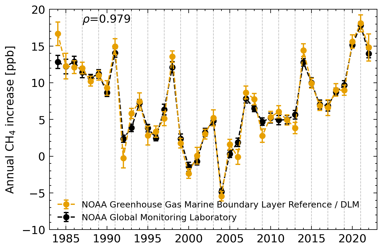
Figure B1Comparison of global annual methane increases derived from the NOAA–GML MBLR data using different methods.
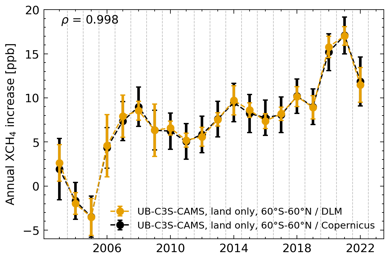
Figure B2Comparison of global annual methane increases derived from C3S XCH4_OBS4MIPS v4.4 data which are extended by CAMS NRT data after 2021 using different methods.
Here we present global AMIs and zonal growth rates for CAMS/INV-SRF-SAT data which includes satellite measurements from GOSAT in its optimization (see Figs. C1 and C2).
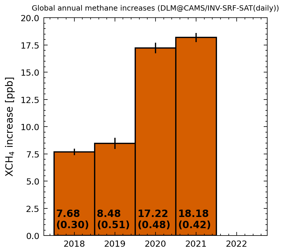
Figure C1Global annual methane increases derived from CAMS global inversion-optimized greenhouse concentrations including both surface and satellite observations.
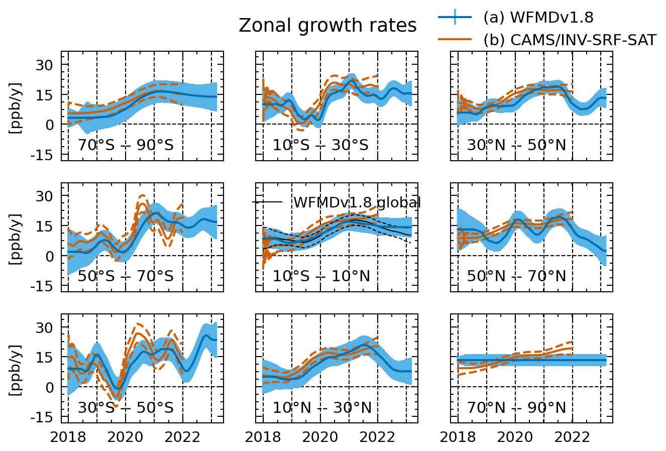
Figure C2Zonal growth rates for 20∘ bands derived from (a) Sentinel-5P TROPOMI WFMDv1.8 data and (b) CAMS/INV-SRF-SAT data. The errors show the 1σ uncertainty.
Figure D1 shows the area-normalized coverage of S5P/TROPOMI WFMDv1.8 data. It can be seen that the tropics, mid-latitudes, and high latitudes mostly have an average coverage of about 25 %, while the high-latitude regions have seasonal gaps due to the polar night.
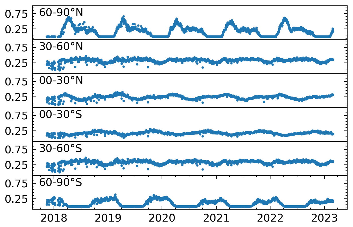
Figure D1Area-normalized coverage of S5P/TROPOMI WFMDv1.8 data for 30∘ zonal bands, representing the high-latitude, mid-latitude, and tropical regions. For the calculation, data on a 2∘ × 2∘ grid were used. The coverage is given on a scale from 0 to 1, where 1 represents complete coverage within a band.
CAMS global inversion-optimized greenhouse gas fluxes and concentrations are available from https://ads.atmosphere.copernicus.eu/ (last access: 21 June 2023, Segers et al., 2022). Sentinel-5P TROPOMI WFMD data are available from https://www.iup.uni-bremen.de/carbon_ghg/products/tropomi_wfmd/ (last access: 28 March 2023, Schneising et al., 2023). NOAA MBL data are available from https://gml.noaa.gov/ccgg/mbl/ (last access: 30 October 2023, Dlugokencky et al., 2021). Example code to recreate Fig. 5 (global annual methane increases), including the gridding and processing of the data, is available at https://doi.org/10.5281/zenodo.8178927 (Hachmeister, 2023).
JH developed the methodology and conducted the formal analysis. OS provided information on the WFMDv1.8 data. MiB provided information on the UB–C3S–CAMS data. JPB provided valuable input on atmospheric transport effects. MaB provided supervision and helped with the conceptualization. JH wrote the initial draft of this paper. All the authors contributed significantly to the conception of the analysis, jointly discussed the results, and provided constructive comments to improve the manuscript.
The contact author has declared that none of the authors has any competing interests.
Publisher's note: Copernicus Publications remains neutral with regard to jurisdictional claims made in the text, published maps, institutional affiliations, or any other geographical representation in this paper. While Copernicus Publications makes every effort to include appropriate place names, the final responsibility lies with the authors.
This publication uses and contains modified Copernicus Atmosphere Monitoring Service information (2018–2022) and modified Copernicus Sentinel data (2018–2023). Sentinel-5 Precursor is an ESA mission implemented on behalf of the European Commission. The TROPOMI payload is a joint development by the European Space Agency (ESA) and the Netherlands Space Office (NSO). The Sentinel-5 Precursor ground-segment development has been funded by the ESA and with national contributions from the Netherlands, Germany, and Belgium. The pre-operational TROPOMI data processing was carried out on the Dutch national e-infrastructure with the support of the SURF cooperative. Scientific colour maps (Crameri, 2021) are used in this study to prevent visual distortion of data and exclusion of readers with colour-vision deficiencies (Crameri et al., 2020).
This project is funded by the State and University of Bremen. In particular, the University of Bremen funding for the junior research group “Greenhouse gases in the Arctic” is acknowledged by Jonas Hachmeister and Michael Buchwitz. We gratefully acknowledge the funding by the Deutsche Forschungsgemeinschaft (DFG, German Research Foundation), grant no. 268020496 – TRR 172, within the Transregional Collaborative Research Center “ArctiC Amplification: Climate Relevant Atmospheric and SurfaCe Processes, and Feedback Mechanisms (AC)3”. We also acknowledge the received funding from the ESA via projects GHG-CCI+ and MethaneCAMP (ESA contract nos. 4000126450/19/I-NB and 4000137895/22/I-AG) and from the German Ministry of Education and Research (BMBF) within its ITMS project via grant no. 01 LK2103A. The TROPOMI/WFMD version 1.8 data have been generated using funding from the ESA (GHG-CCI and MethaneCAMP projects). The TROPOMI/WFMD retrievals presented here were performed at HPC facilities of the IUP, University of Bremen, funded under DFG/FUGG grant nos. INST 144/379-1 and INST 144/493-1. Some of the AMIs presented were generated for Copernicus ESOTC 2022 (https://climate.copernicus.eu/climate-indicators/greenhouse-gas-concentrations, last access: 30 June 2023) funded by the EU Copernicus Climate Change Service via project no. C3S2_ 312a_Lot2.
The article processing charges for this open-access publication were covered by the University of Bremen.
This paper was edited by Bryan N. Duncan and reviewed by two anonymous referees.
Arias, P., Bellouin, N., Coppola, E., Jones, R., Krinner, G., Marotzke, J., Naik, V., Palmer, M., Plattner, G.-K., Rogelj, J., Rojas, M., Sillmann, J., Storelvmo, T., Thorne, P., Trewin, B., Achuta Rao, K., Adhikary, B., Allan, R., Armour, K., Bala, G., Barimalala, R., Berger, S., Canadell, J., Cassou, C., Cherchi, A., Collins, W., Collins, W., Connors, S., Corti, S., Cruz, F., Dentener, F., Dereczynski, C., Di Luca, A., Diongue Niang, A., Doblas-Reyes, F., Dosio, A., Douville, H., Engelbrecht, F., Eyring, V., Fischer, E., Forster, P., Fox-Kemper, B., Fuglestvedt, J., Fyfe, J., Gillett, N., Goldfarb, L., Gorodetskaya, I., Gutierrez, J., Hamdi, R., Hawkins, E., Hewitt, H., Hope, P., Islam, A., Jones, C., Kaufman, D., Kopp, R., Kosaka, Y., Kossin, J., Krakovska, S., Lee, J.-Y., Li, J., Mauritsen, T., Maycock, T., Meinshausen, M., Min, S.-K., Monteiro, P., Ngo-Duc, T., Otto, F., Pinto, I., Pirani, A., Raghavan, K., Ranasinghe, R., Ruane, A., Ruiz, L., Sallée, J.-B., Samset, B., Sathyendranath, S., Seneviratne, S., Sörensson, A., Szopa, S., Takayabu, I., Tréguier, A.-M., van den Hurk, B., Vautard, R., von Schuckmann, K., Zaehle, S., Zhang, X., and Zickfeld, K.: Technical Summary, in: Climate Change 2021: The Physical Science Basis. Contribution of Working Group I to the Sixth Assessment Report of the Intergovernmental Panel on Climate Change, edited by: Masson-Delmotte, V., Zhai, P., Pirani, A., Connors, S., Péan, C., Berger, S., Caud, N., Chen, Y., Goldfarb, L., Gomis, M., Huang, M., Leitzell, K., Lonnoy, E., Matthews, J., Maycock, T., Waterfield, T., Yelekçi, O., Yu, R., and Zhou, B.: Cambridge University Press, Cambridge, United Kingdom and New York, NY, USA, https://doi.org/10.1017/9781009157896.002, p. 33–144, 2021. a
Basu, S., Lan, X., Dlugokencky, E., Michel, S., Schwietzke, S., Miller, J. B., Bruhwiler, L., Oh, Y., Tans, P. P., Apadula, F., Gatti, L. V., Jordan, A., Necki, J., Sasakawa, M., Morimoto, S., Di Iorio, T., Lee, H., Arduini, J., and Manca, G.: Estimating emissions of methane consistent with atmospheric measurements of methane and δ13C of methane, Atmos. Chem. Phys., 22, 15351–15377, https://doi.org/10.5194/acp-22-15351-2022, 2022. a
Bergamaschi, P., Krol, M., Meirink, J. F., Dentener, F., Segers, A., van Aardenne, J., Monni, S., Vermeulen, A. T., Schmidt, M., Ramonet, M., Yver, C., Meinhardt, F., Nisbet, E. G., Fisher, R. E., O'Doherty, S., and Dlugokencky, E. J.: Inverse modeling of European CH4 emissions 2001–2006, J. Geophys. Res.-Atmos., 115, D22309, https://doi.org/10.1029/2010JD014180, 2010. a
Bergamaschi, P., Houweling, S., Segers, A., Krol, M., Frankenberg, C., Scheepmaker, R. A., Dlugokencky, E., Wofsy, S. C., Kort, E. A., Sweeney, C., Schuck, T., Brenninkmeijer, C., Chen, H., Beck, V., and Gerbig, C.: Atmospheric CH4 in the first decade of the 21st century: Inverse modeling analysis using SCIAMACHY satellite retrievals and NOAA surface measurements, J. Geophys. Res.-Atmos., 118, 7350–7369, 2013. a
Buchwitz, M., Schneising, O., Reuter, M., Heymann, J., Krautwurst, S., Bovensmann, H., Burrows, J. P., Boesch, H., Parker, R. J., Somkuti, P., Detmers, R. G., Hasekamp, O. P., Aben, I., Butz, A., Frankenberg, C., and Turner, A. J.: Satellite-derived methane hotspot emission estimates using a fast data-driven method, Atmos. Chem. Phys., 17, 5751–5774, https://doi.org/10.5194/acp-17-5751-2017, 2017. a, b
Cooper, M. J., Martin, R. V., Hammer, M. S., Levelt, P. F., Veefkind, P., Lamsal, L. N., Krotkov, N. A., Brook, J. R., and McLinden, C. A.: Global fine-scale changes in ambient NO2 during COVID-19 lockdowns, Nature, 601, 380–387, https://doi.org/10.1038/s41586-021-04229-0, 2022. a
Copernicus Atmosphere Monitoring Service: https://atmosphere.copernicus.eu/ (last access: 30 June 2023), 2023. a
Copernicus Climate Change Service, Climate Data Store: Methane data from 2002 to present derived from satellite observations, Climate Data Store (CDS) [data set], https://doi.org/10.24381/CDS.B25419F8, 2018. a
Copernicus Climate Change Service: https://climate.copernicus.eu/ (last access: 30 June 2023), 2023a. a
Copernicus Climate Change Service: Climate Data Store, https://cds.climate.copernicus.eu/#!/home (last access: 30 June 2023), 2023b. a
Copernicus Climate Change Service: Climate Indicators – Greenhouse gas concentrations https://climate.copernicus.eu/climate-indicators/greenhouse-gas-concentrations (last access: 30 June 2023), 2023c. a, b, c, d, e, f
Copernicus Climate Change Service: European State of the Climate 2022, https://climate.copernicus.eu/esotc/2022 (last access: 30 June 2023), 2023d. a
Crameri, F.: Scientific colour maps, Zenodo, https://doi.org/10.5281/zenodo.5501399, 2021. a
Crameri, F., Shephard, G. E., and Heron, P. J.: The misuse of colour in science communication, Nat. Commun., 11, 5444, https://doi.org/10.1038/s41467-020-19160-7, 2020. a
Dlugokencky, E.: Trends in Atmospheric Methane, https://www.gml.noaa.gov/ccgg/trends_ch4/ (last access: 20 September 2022), 2022. a, b
Dlugokencky, E. J., Lan, X., Crotwell, A., Thoning, K., and Crotwell, M.: Atmospheric Methane Dry Air Mole Fractions from the NOAA ESRL Carbon Cycle Cooperative Global Air Sampling Network [data set], ftp://aftp.cmdl.noaa.gov/data/trace_gases/ch4/flask/surface/ (last access: 30 October 2023), 2021. a, b
Durbin, J. and Koopman, S. J.: Time Series analysis by state space methods, 2nd Edition, Oxford University Press, Oxford University Press, https://doi.org/10.1093/acprof:oso/9780199641178.001.000, 2012. a, b, c
Feng, L., Palmer, P. I., Zhu, S., Parker, R. J., and Liu, Y.: Tropical methane emissions explain large fraction of recent changes in global atmospheric methane growth rate, Nat. Commun., 13, 1378, https://doi.org/10.1038/s41467-022-28989-z, 2022. a, b, c
Feng, L., Palmer, P. I., Parker, R. J., Lunt, M. F., and Bösch, H.: Methane emissions are predominantly responsible for record-breaking atmospheric methane growth rates in 2020 and 2021, Atmos. Chem. Phys., 23, 4863–4880, https://doi.org/10.5194/acp-23-4863-2023, 2023. a, b, c, d, e, f, g, h, i, j, k, l, m, n, o, p
Global Methane Tracker 2021: license: CC BY 4.0, https://www.iea.org/reports/methane-tracker-2021 (last access: 20 July 2023), 2021. a, b
Global Methane Tracker 2022: license: CC BY 4.0, https://www.iea.org/reports/global-methane-tracker-2022 (last access: 20 July 2023), 2023. a
Gulev, S., Thorne, P., Ahn, J., Dentener, F., Domingues, C., Gerland, S., Gong, D., Kaufman, D., Nnamchi, H., Quaas, J., Rivera, J., Sathyendranath, S., Smith, S., Trewin, B., von Schuckmann, K., and Vose, R.: Changing State of the Climate System, in: Climate Change 2021: The Physical Science Basis. Contribution of Working Group I to the Sixth Assessment Report of the Intergovernmental Panel on Climate Change, edited by: Masson-Delmotte, V., Zhai, P., Pirani, A., Connors, S., Péan, C., Berger, S., Caud, N., Chen, Y., Goldfarb, L., Gomis, M., Huang, M., Leitzell, K., Lonnoy, E., Matthews, J., Maycock, T., Waterfield, T., Yelekçi, O., Yu, R., and Zhou, B., Cambridge University Press, Cambridge, United Kingdom and New York, NY, USA, https://doi.org/10.1017/9781009157896.004, pp. 287–422, 2021. a
Hachmeister, J.: Calculating global annual methane increases from satellite data using an ensemble dynamic linear model approach (1.0.0), Zenodo [code], https://doi.org/10.5281/zenodo.8178927, 2023. a
Hachmeister, J., Schneising, O., Buchwitz, M., Lorente, A., Borsdorff, T., Burrows, J. P., Notholt, J., and Buschmann, M.: On the influence of underlying elevation data on Sentinel-5 Precursor TROPOMI satellite methane retrievals over Greenland, Atmos. Meas. Tech., 15, 4063–4074, https://doi.org/10.5194/amt-15-4063-2022, 2022. a
Harvey, A. C.: Forecasting, Structural Time Series Models and the Kalman Filter, Cambridge University Press, https://doi.org/10.1017/CBO9781107049994, 1990. a, b, c
Hugelius, G., Strauss, J., Zubrzycki, S., Harden, J. W., Schuur, E. A. G., Ping, C.-L., Schirrmeister, L., Grosse, G., Michaelson, G. J., Koven, C. D., O'Donnell, J. A., Elberling, B., Mishra, U., Camill, P., Yu, Z., Palmtag, J., and Kuhry, P.: Estimated stocks of circumpolar permafrost carbon with quantified uncertainty ranges and identified data gaps, Biogeosciences, 11, 6573–6593, https://doi.org/10.5194/bg-11-6573-2014, 2014. a
Jacob, D. J.: Introduction to Atmospheric Chemistry, Princeton University Press, https://doi.org/10.1515/9781400841547, 1999. a, b
Karppinen, T., Lamminpää, O., Tukiainen, S., Kivi, R., Heikkinen, P., Hatakka, J., Laine, M., Chen, H., Lindqvist, H., and Tamminen, J.: Vertical Distribution of Arctic Methane in 2009–2018 Using Ground-Based Remote Sensing, Remote Sens.-Basel, 12, 917, https://doi.org/10.3390/rs12060917, 2020. a
Kivimäki, E., Lindqvist, H., Hakkarainen, J., Laine, M., Sussmann, R., Tsuruta, A., Detmers, R., Deutscher, N. M., Dlugokencky, E. J., Hase, F., Hasekamp, O., Kivi, R., Morino, I., Notholt, J., Pollard, D. F., Roehl, C., Schneider, M., Sha, M. K., Velazco, V. A., Warneke, T., Wunch, D., Yoshida, Y., and Tamminen, J.: Evaluation and Analysis of the Seasonal Cycle and Variability of the Trend from GOSAT Methane Retrievals, Remote Sens.-Basel, 11, 882, https://doi.org/10.3390/rs11070882, 2019. a
Laine, M.: Introduction to Dynamic Linear Models for Time Series Analysis, in: Geodetic Time Series Analysis in Earth Sciences, Springer International Publishing, Cham, 139–156, https://doi.org/10.1007/978-3-030-21718-1_4, 2020. a, b
Laine, M., Latva-Pukkila, N., and Kyrölä, E.: Analysing time-varying trends in stratospheric ozone time series using the state space approach, Atmos. Chem. Phys., 14, 9707–9725, https://doi.org/10.5194/acp-14-9707-2014, 2014. a
Lan, X., Basu, S., Schwietzke, S., Bruhwiler, L. M. P., Dlugokencky, E. J., Michel, S. E., Sherwood, O. A., Tans, P. P., Thoning, K., Etiope, G., Zhuang, Q., Liu, L., Oh, Y., Miller, J. B., Pétron, G., Vaughn, B. H., and Crippa, M.: Improved Constraints on Global Methane Emissions and Sinks Using δ13C-CH4, Global Biogeochem. Cy., 35, e2021GB007000, https://doi.org/10.1029/2021GB007000, 2021. a
Lan, X., Thoning, K., and Dlugokencky, E. J.: Trends in globally-averaged CH4, N2O, and SF6 determined from NOAA Global Monitoring Laboratory measurements, Version 2023-10, NOAA Global Monitoring Laboratory [data set], https://doi.org/10.15138/P8XG-AA10, 2023. a, b, c
Laughner, J. L., Neu, J. L., Schimel, D., Wennberg, P. O., Barsanti, K., Bowman, K. W., Chatterjee, A., Croes, B. E., Fitzmaurice, H. L., Henze, D. K., Kim, J., Kort, E. A., Liu, Z., Miyazaki, K., Turner, A. J., Anenberg, S., Avise, J., Cao, H., Crisp, D., de Gouw, J., Eldering, A., Fyfe, J. C., Goldberg, D. L., Gurney, K. R., Hasheminassab, S., Hopkins, F., Ivey, C. E., Jones, D. B. A., Liu, J., Lovenduski, N. S., Martin, R. V., McKinley, G. A., Ott, L., Poulter, B., Ru, M., Sander, S. P., Swart, N., Yung, Y. L., and Zeng, Z.-C.: Societal shifts due to COVID-19 reveal large-scale complexities and feedbacks between atmospheric chemistry and climate change, P. Natl. Acad. Sci. USA, 118, e2109481118, https://doi.org/10.1073/pnas.2109481118, 2021. a, b, c
Ludewig, A.: S5P Mission Performance Centre Level 1b Readme, https://sentinels.copernicus.eu/documents/247904/3541451/Sentinel-5P-Level-1b-Product-Readme-File.pdf/a89d82ce-7414-43e6-ac77-0c371ed1b096 (last access: 30 November 2023), 2021. a
McNorton, J., Bousserez, N., Agustí-Panareda, A., Balsamo, G., Cantarello, L., Engelen, R., Huijnen, V., Inness, A., Kipling, Z., Parrington, M., and Ribas, R.: Quantification of methane emissions from hotspots and during COVID-19 using a global atmospheric inversion, Atmos. Chem. Phys., 22, 5961–5981, https://doi.org/10.5194/acp-22-5961-2022, 2022. a
NOAA Greenhouse Gas Marine Boundary Layer Reference – Documentation: https://gml.noaa.gov/ccgg/mbl/mbl.html, last access: 30 October 2023. a
Peng, S., Lin, X., Thompson, R. L., Xi, Y., Liu, G., Hauglustaine, D., Lan, X., Poulter, B., Ramonet, M., Saunois, M., Yin, Y., Zhang, Z., Zheng, B., and Ciais, P.: Wetland emission and atmospheric sink changes explain methane growth in 2020, Nature, 612, 477–482, https://doi.org/10.1038/s41586-022-05447-w, 2022. a, b, c, d, e, f, g, h, i, j, k, l
Perktold, J., Skipper Seabold, Sheppard, K., ChadFulton, Kerby Shedden, Jbrockmendel, J-Grana6, Quackenbush, P., Arel-Bundock, V., McKinney, W., Langmore, I., Baker, B., Gommers, R., Yogabonito, S-Scherrer, Zhurko, E., Brett, M., Giampieri, E., Yichuan Liu, Millman, J., Hobson, P., Vincent, Roy, P., Augspurger, T., Tvanzyl, Alexbrc, Hartley, T., Perez, F., Tamiya, Y., and Halchenko, Y.: statsmodels/statsmodels: Release 0.14.0, Zenodo [code], https://doi.org/10.5281/ZENODO.593847, 2023. a
Plaza, C., Pegoraro, E., Bracho, R., Celis, G., Crummer, K. G., Hutchings, J. A., Hicks Pries, C. E., Mauritz, M., Natali, S. M., Salmon, V. G., Schädel, C., Webb, E. E., and Schuur, E. A. G.: Direct observation of permafrost degradation and rapid soil carbon loss in tundra, Nat. Geosci., 12, 627–631, https://doi.org/10.1038/s41561-019-0387-6, 2019. a
Qu, Z., Jacob, D. J., Zhang, Y., Shen, L., Varon, D. J., Lu, X., Scarpelli, T., Bloom, A., Worden, J., and Parker, R. J.: Attribution of the 2020 surge in atmospheric methane by inverse analysis of GOSAT observations, Environ. Res. Lett., 17, 094003, https://doi.org/10.1088/1748-9326/ac8754, 2022. a, b, c, d, e, f, g, h, i, j, k
Reuter, M., Buchwitz, M., Schneising, O., Noël, S., Bovensmann, H., Burrows, J. P., Boesch, H., Di Noia, A., Anand, J., Parker, R. J., Somkuti, P., Wu, L., Hasekamp, O. P., Aben, I., Kuze, A., Suto, H., Shiomi, K., Yoshida, Y., Morino, I., Crisp, D., O'Dell, C. W., Notholt, J., Petri, C., Warneke, T., Velazco, V. A., Deutscher, N. M., Griffith, D. W. T., Kivi, R., Pollard, D. F., Hase, F., Sussmann, R., Té, Y. V., Strong, K., Roche, S., Sha, M. K., De Mazière, M., Feist, D. G., Iraci, L. T., Roehl, C. M., Retscher, C., and Schepers, D.: Ensemble-based satellite-derived carbon dioxide and methane column-averaged dry-air mole fraction data sets (2003–2018) for carbon and climate applications, Atmos. Meas. Tech., 13, 789–819, https://doi.org/10.5194/amt-13-789-2020, 2020. a, b
Schneising, O., Buchwitz, M., Hachmeister, J., Vanselow, S., Reuter, M., Buschmann, M., Bovensmann, H., and Burrows, J. P.: Advances in retrieving XCH4 and XCO from Sentinel-5 Precursor: improvements in the scientific TROPOMI/WFMD algorithm, Atmos. Meas. Tech., 16, 669–694, https://doi.org/10.5194/amt-16-669-2023, 2023. a, b, c, d, e, f, g
Segers, A., Steinke, T., and Houweling, S.: Description of the CH4 Inversion Production Chain, https://atmosphere.copernicus.eu/sites/default/files/2022-10/CAMS255_2021SC1_D55.5.2.1-2021CH4_202206_production_chain_CH4_v1.pdf (last access: 25 June 2023), 2022. a, b
Serreze, M. C. and Barry, R. G.: Processes and impacts of Arctic amplification: A research synthesis, Global Planet. Change, 77, 85–96, https://doi.org/10.1016/j.gloplacha.2011.03.004, 2011. a
Sofieva, V. F., Kalakoski, N., Päivärinta, S.-M., Tamminen, J., Laine, M., and Froidevaux, L.: On sampling uncertainty of satellite ozone profile measurements, Atmos. Meas. Tech., 7, 1891–1900, https://doi.org/10.5194/amt-7-1891-2014, 2014. a, b
statsmodels 0.14.0 documentation: UnobservedComponents class https://www.statsmodels.org/stable/generated/statsmodels.tsa.statespace.structural.UnobservedComponents.html (last access: 8 December 2023), 2023. a
Stevenson, D. S., Derwent, R. G., Wild, O., and Collins, W. J.: COVID-19 lockdown emission reductions have the potential to explain over half of the coincident increase in global atmospheric methane, Atmos. Chem. Phys., 22, 14243–14252, https://doi.org/10.5194/acp-22-14243-2022, 2022. a, b, c
Szopa, S., Naik, V., Adhikary, B., Artaxo, P., Berntsen, T., Collins, W., Fuzzi, S., Gallardo, L., Kiendler-Scharr, A., Klimont, Z., Liao, H., Unger, N., and Zanis, P.: Short-Lived Climate Forcers, in: Climate Change 2021: The Physical Science Basis. Contribution of Working Group I to the Sixth Assessment Report of the Intergovernmental Panel on Climate Change, edited by: Masson-Delmotte, V., Zhai, P., Pirani, A., Connors, S., Péan, C., Berger, S., Caud, N., Chen, Y., Goldfarb, L., Gomis, M., Huang, M., Leitzell, K., Lonnoy, E., Matthews, J., Maycock, T., Waterfield, T., Yelekçi, O., Yu, R., and Zhou, B., Cambridge University Press, Cambridge, United Kingdom and New York, NY, USA, https://doi.org/10.1017/9781009157896.008, pp. 817–922, 2021. a, b
Turner, A. J., Frankenberg, C., and Kort, E. A.: Interpreting contemporary trends in atmospheric methane, P. Natl. Acad. Sci. USA, 116, 2805–2813, https://doi.org/10.1073/pnas.1814297116, 2019. a
Warneck, P.: Chemistry of the Natural Atmosphere, 2nd Edn., vol. 71 of INTERNATIONAL GEOPHYSICS SERIES, Academic Press, ISBN 0-12-735632-0, 1999. a, b
Wendisch, M., Brückner, M., Burrows, J. P., Crewell, S., Dethloff, K., Ebell, K., Lüpkes, C., Macke, A., Notholt, J., Quaas, J., Rinke, A., and Tegen, I.: Understanding Causes and Effects of Rapid Warming in the Arctic, EOS, 98, https://doi.org/10.1029/2017EO064803, 2017. a
Zhang, Z., Poulter, B., Feldman, A. F., Ying, Q., Ciais, P., Peng, S., and Li, X.: Recent intensification of wetland methane feedback, Nat. Clim. Change, 13, 430–433, https://doi.org/10.1038/s41558-023-01629-0, 2023. a, b
- Abstract
- Introduction
- Data
- Method
- Comparison of different global annual methane increases
- Investigation of zonal methane growth rates
- CAMS/INV fluxes
- Conclusions
- Appendix A: Model set-up and ensemble size
- Appendix B: Replication of complete NOAA GML and UB–C3S AMIs
- Appendix C: Global AMIs and zonal growth rates derived from CAMS global inversion-optimized greenhouse concentrations
- Appendix D: WFMDv1.8 data coverage
- Code and data availability
- Author contributions
- Competing interests
- Disclaimer
- Acknowledgements
- Financial support
- Review statement
- References