Summertime tropospheric ozone source apportionment study in the Madrid region (Spain)

The design of emission abatement measures to effectively reduce high ground-level ozone (O₃) concentrations in urban areas is very complex. In addition to the strongly non-linear chemistry of this secondary pollutant, precursors can be released by a variety of sources in different regions, and locally produced O₃ is mixed with that transported from the regional or continental scales. All of these processes depend also on the specific meteorological conditions and topography of the study area. Consequently, high-resolution comprehensive modeling tools are needed to understand the drivers of photochemical pollution and to assess the potential of local strategies to reduce adverse impacts from high tropospheric O₃ levels. In this study, we apply the Integrated Source Apportionment Method (ISAM) implemented in the Community Multiscale Air Quality (CMAQ v5.3.2) model to investigate the origin of summertime O₃ in the Madrid region (Spain). Consistent with previous studies, our results confirm that O₃ levels are dominated by non-local contributions, representing around 70 % of mean values across the region. Nonetheless, precursors emitted by local sources, mainly road traffic, play a more important role during O₃ peaks, with contributions as high as 25 ppb. The potential impact of local measures is higher under unfavorable meteorological conditions associated with regional accumulation patterns. These findings suggest that this modeling system may be used in the future to simulate the potential outcomes of specific emission abatement measures to prevent high-O₃ episodes in the Madrid metropolitan area.

1 Introduction

Air pollution is one of the main environmental problems and is recognized as a global threat to public health. In 2019, 4.2 million people died prematurely worldwide as a result of poor air quality (WHO, 2021). Even in regions that have taken decisive actions to curb emissions, such as Europe, over 300 000 premature deaths (EU27) are currently attributed to air pollution, most of them related to high levels of PM_2.5 (particles with an aerodynamic diameter of ≤ 2.5 µm) (238 000) and NO₂ (nitrogen dioxide) (49 000) (EEA, 2022). In recent years, concentrations of many of the regulated pollutants in Europe have decreased as a result of a general reduction in emissions. From 2009 to 2018, the concentration of PM₁₀ (particles with an aerodynamic diameter of ≤ 10 µm), PM_2.5, and NO₂ diminished on average by 19 %, 22 %, and 18 %–23 % (depending on the air quality monitoring station type), respectively (EEA, 2020). These measures, however, have not reported comparable reductions in ozone (O₃) ambient concentration levels.

Tropospheric O₃ is a secondary pollutant formed from photochemical reactions between many different precursors, mainly nitrogen oxides (${\mathrm{NO}}_x=\mathrm{NO}\left(\text{nitric oxide}\right)+{\mathrm{NO}}_{\mathrm{2}}$) and non-methane volatile organic compounds (VOCs) (Seinfeld and Pandis, 2016; Jenkin and Clemitshaw, 2000; Monks et al., 2015). According to the last European Union (EU) emission inventory report (EEA, 2022), the most important activity sectors regarding O₃ precursor emissions are the “Road transport” sector (7 % and 37 % of total VOCs and NO_X emissions, respectively), the “Commercial, institutional and households” sector (15 % and 14 %, respectively), and the “Solvent and product use” sector, representing 42 % of total VOC emissions. Once emitted from urban and industrial areas, these precursors are subsequently transported by the prevailing wind regime (Xu et al., 2011). The atmospheric lifetime of O₃ depends on numerous variables. In the boundary layer, the atmospheric lifetime of O₃ is short, roughly 1 or 2 d, depending on the abundance of precursors (Young et al., 2013). In the free troposphere, its lifetime can be up to 2 weeks, time enough to be transported long distances, from the local to the global scale (Monks et al., 2015; Stevenson et al., 2006). In addition to in situ formation, transport of O₃ from the stratosphere is relevant to explain the tropospheric ozone levels (IPCC, 2007; Hsu et al., 2005). Furthermore, this gas exchange between layers of the atmosphere is expected to increase in the future globally (Meul et al., 2018; Banerjee et al., 2016) due to dynamic and chemical changes in the atmosphere induced by climate change.

Due to these complex dynamics, tropospheric O₃ levels have not decreased (Jung et al., 2022; Sicard et al., 2023) in accordance with significant NO_X and VOC emissions reduction (45 % and 41 %, respectively, during 2009–2018). As a result, 12 % of the urban population in Europe is still exposed to high O₃ concentrations according to EU regulations, with a toll of 24 000 premature annual deaths (EEA, 2022), especially in the Mediterranean basin (Amann et al., 2008; European Environment Agency et al., 2018; EEA, 2020). The share of urban population that suffers from excessive exposure to O₃ rises to 95 % (EEA, 2022) when the World Health Organization (WHO) guidelines are considered (WHO, 2021). Of note, tropospheric O₃ produces both short-term (Bates et al., 1972; Bell et al., 2004; Goodman et al., 2018) and long-term health effects (Jerrett et al., 2009; Seltzer et al., 2018), impacting the population living in large urban agglomerations as well as their surroundings. Moreover, it also may have relevant effects on ecosystems (De Andrés et al., 2012; Mills et al., 2011; Harmens et al., 2011) and climate (Sitch et al., 2007; Stocker et al., 2013; IPCC, 2014).

Globally, the latest studies using satellite data suggest that tropospheric O₃ average levels increased over the past four decades (Ziemke et al., 2019; Gaudel et al., 2018). Paoletti et al. (2014) evaluated observations from monitoring stations in the United States (US) and Europe from 1990 to 2010 and concluded that the O₃ annual average increased by 7 % yr⁻¹ in rural stations and around 12 % yr⁻¹–17 % yr⁻¹ (US and EU, respectively) in urban stations. However, O₃ formation is highly non-linear and trends may change depending on the evaluated time period and region, the metric used, and other local factors such as topography or the proximity to the precursor's emission sources (Reche et al., 2018; Massagué et al., 2023). According to specific studies for the Iberian Peninsula, the trend of the annual average of O₃ for rural stations during 2004–2012 was not clear (Querol et al., 2014). In contrast, an increasing trend around 1 % yr⁻¹–3 % yr⁻¹ was observed in all seasons in urban, traffic, and industrial stations. Borge et al. (2019) reported an average increase of 10 µg m⁻³ in daily 8 h maximum O₃ moving average concentrations (MDA8) for 1993–2017. However, they detected that the highest increase was related to fall and winter (up to 19 µg m⁻³), in agreement with general increases in the oxidation capacity in the atmosphere of the largest urban areas in Europe modeled by Jung et al. (2022).

Nonetheless, the O₃-forming photochemical activity is largely regulated by weather conditions, especially temperature and solar radiation. For this reason, tropospheric O₃ formation has a marked seasonal character, with the highest O₃ values typically recorded in spring and summer (Logan, 1985; Granados-Muñoz and Leblanc, 2016), especially in those locations that are highly influenced by nearby urban areas (Brodin et al., 2010; Carnero et al., 2009) where large amounts of precursors are emitted. Therefore, understanding summertime O₃ dynamics is more relevant from an air quality management perspective. Furthermore, information on the relative importance of emission sources on ambient levels should be considered when designing plans and measures, especially when they target highly non-linear secondary pollutants such as O₃ (Cohan and Napelenok, 2011).

There are different source apportionment techniques that may support air pollution research and decision making (Thunis et al., 2019). Approaches based on sensitivities, such as single-perturbation or brute force methods (Borge et al., 2014; Tagaris et al., 2014; Zhang et al., 2022; Qu et al., 2023), may be useful in anticipating the potential effect of a given intervention. However, tagging methods (Grewe et al., 2017; Butler et al., 2018) provide fully mass conservative apportionment at receptors of interest and may be better suited for diagnostic purposes (Borge et al., 2022). These pollution tracking capabilities have been integrated into modern air quality models to provide attribution information together with the standard concentration and deposition output fields, and can be successfully applied to study pollution dynamics (Simon et al., 2018; Pay et al., 2019; Li et al., 2022). This approach may be particularly interesting to describe how O₃ levels are linked to emission sources under unfavorable meteorological conditions (Cao et al., 2022; Zohdirad et al., 2022) or specific local atmospheric circulation patterns (Zhang et al., 2023) that may lead to high concentration events (Lupaşcu et al., 2022).

This research focuses on the center of the Iberian Peninsula, encompassing the city of Madrid and its surroundings. Consistently with general emission trends in Europe, the emission of the main O₃ precursors in the Madrid region decreased by 47 % for VOCs and 44 % for NO_X from 1990 to 2018 (CM, 2021). While recent control measures succeeded in reducing NO₂ levels (AM, 2022), such emission reductions have, at the same time, substantially impacted urban atmospheric chemistry by modifying its oxidative capacity. Recent studies (Saiz-Lopez et al., 2017; Querol et al., 2016) suggest that O₃ levels increased in Madrid by 30 %–40 % during 2007–2014. A greater decrease in NO emissions than in NO₂ emissions (with a subsequent reduction in the $\mathrm{NO}/{\mathrm{NO}}_{\mathrm{2}}$ ratio) may be one of the factors responsible for this response (Querol et al., 2016, 2017; Zaveri et al., 2003; Jhun et al., 2015). The exceedances of the target value for the protection of human health in the region mainly occur in summer, especially under adverse meteorological conditions that have been extensively characterized in previous studies (Querol et al., 2016, 2017, 2018; Millán et al., 2000; Plaza et al., 1997; Pay et al., 2019; Escudero et al., 2019). Preventing these exceedances in the region requires an understanding of the source attribution of O₃, especially under specific weather patterns that may lead to high pollution levels (Zhang et al., 2023).

In this research, we apply a state-of-the-science air quality model to provide insights into the emission sources and transport patterns which are involved in the formation of tropospheric O₃ during typical summertime conditions in the Madrid region. In addition to contributing to the scientific understanding of photochemical pollution, the final purpose of this work is to inform the decision-making process needed to design further emission reduction measures in the study area.

2 Methodology

2.1 Modeling system

The research is supported by a mesoscale modeling system with three main components. Meteorological fields are generated by Weather Research and Forecasting (WRF v3.7.1) (Skamarock and Klemp, 2008). Physics options and parameterizations (Table S1 in the Supplement) are based on previous studies (Borge et al., 2008a; de la Paz et al., 2016), and WRF outputs are postprocessed with the Meteorology–Chemistry Interface Processor (MCIP v5.1) (Otte and Pleim, 2010). Emission processing relies on the US Environmental Protection Agency's (EPA) Sparse Matrix Operator Kernel System (SMOKE v3.6.5) model (UNC, 2015; Baek and Seppanen, 2018) which has been specifically adapted for the Iberian Peninsula (Borge et al., 2008b, 2014). Biogenic emissions are generated by Model Emissions Gases and Aerosols from Nature (MEGAN v2.1) (Guenther, 2006; Guenther et al., 2012). The third component is the Community Multiscale Air Quality (CMAQ v5.3.2) modeling system (Byun and Schere, 2006; Ching and Byun, 1999). This 3D chemical-transport model (CTM) simultaneously predicts the concentration of all relevant substances considering transport (advection and diffusion), chemical transformation, and deposition. Gas-phase atmospheric chemistry is represented by the Carbon Bond 6 (CB06) (Yarwood et al., 2010) chemical mechanism with chlorine chemistry (CB06r3) (Sarwar et al., 2012; Whitten et al., 2010, Emery et al., 2015) according to SPECIATE 4.0 (Hsu et al., 2006), while the module AERO6 (Appel et al., 2013) is used to describe aerosol dynamics and chemistry. Considering the influence of different scales, from the continental to the regional–urban, on O₃ levels (Valverde et al., 2016; Pay et al., 2019; Baker et al., 2016; Han et al., 2018), boundary conditions (BCs) are of particular interest. Previous studies in the Iberian Peninsula have demonstrated that O₃ is particularly sensitive to boundary conditions (Borge et al., 2010). For a more realistic representation of the boundary influence, the mother domain receives 1 h-resolution, dynamic chemical boundary conditions from hemispheric CMAQ (Mathur et al., 2017) simulations.

In this study, the Integrated Source Apportionment Method (ISAM) (Kwok et al., 2013) implemented in CMAQ v5.3.2 (Napelenok, 2020; Shu et al., 2023) is used. ISAM provides apportionment capability of the full concentration and deposition output arrays including the gaseous photochemically active species, such as O₃, as well as inorganic and organic particulate matter. The CMAQ-ISAM implementation used in this study attributes source identity to secondary pollutants based strictly on reaction stoichiometry with all reactions playing a role that is relevant to the formation and destruction of any species in the chemical mechanism. ISAM is highly customizable for any number of user-specified combinations of emission source sectors and geographical source areas. For O₃, this implementation differs from the previous ISAM versions (including CMAQ v5.0.2) that attribute the formation of secondary pollutants to source sectors based on chemical regime – NO_X- or VOC-limited O₃ formation (Kwok et al., 2015) – and from other studies where precursor attribution is directed by the user to either NO_X or VOC emissions, such as in Butler et al. (2020). Regime-based methods are useful in attributing secondary species that depend on multiple precursors. However, regime determination relies on predefined thresholds of different metrics, often the ${\mathrm{H}}_{\mathrm{2}}{\mathrm{O}}_{\mathrm{2}}/{\mathrm{HNO}}_{\mathrm{3}}$ ratio (Sillman, 1995), that dynamically depend on location and time-specific parameters (Li et al., 2022). By strictly following the stoichiometry of all chemical reactions in the mechanism, this version of ISAM avoids the general necessity of making decisions and assumptions regarding ozone formation regimes. Decisions on tagging method selections are highly dependent on the specific application and the scientific and/or regulatory aims of each individual study. As the needs of the scientific and regulatory communities evolve, so do the apportionment methodologies. Since the conclusion of this work, CMAQ-ISAM has been expanded to include regime-based, stoichiometry-based, and other configuration options. (More information on ISAM as well as sample application and comparison results can be found in Shu et al., 2023.)

2.2 Modeling domains

The three nested domains shown in Fig. 1 were used to perform numerical simulations in this study. This layout is intended to capture medium (Millán et al., 2000) and long-range influences of O₃ transport (Zhang et al., 2020; Qu et al., 2021; Brook et al., 2013), as well as to provide enough resolution over the area of interest to depict local dynamics (Plaza et al., 1997; Borge et al., 2022). The mother domain (D1) includes Europe and northern Africa with a 12 ×12 km spatial resolution, while D2 is centered over the Iberian Peninsula and has a 4 ×4 km spatial resolution (Table S2). The innermost domain (D3) used in this study covers Madrid and surrounding areas with 1 km² spatial resolution (136 km in the east–west direction and 144 km in the north–south direction). All three domains have a common 35-level vertical structure covering the whole troposphere with 18 layers within the first kilometer to accurately represent atmospheric processes within the planetary boundary layer (Borge et al., 2010).

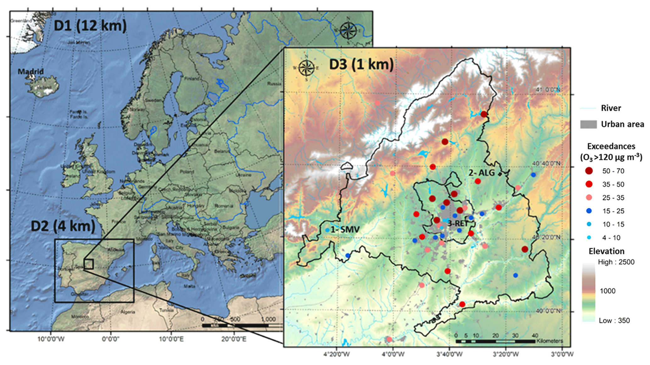
Figure 1 Modeling domains including the location of the air quality monitoring stations within the innermost domain and number of exceedances of the O₃ target value for protection of human health (MDA8 > 120 µg m⁻³) in 2016.

The region has a continental Mediterranean climate with an annual mean temperature of 14.6 °C and 367 mm of accumulated precipitation with a typical summer drought (https://www.madrid.org/iestadis/fijas/coyuntu/otros/cltempe.htm; last access: 10 May 2023). The Central Range (Sierra de Guadarrama), with maximum elevations of 2500 m above sea level (m a.s.l.), crosses the D3 modeling domain in the NE–SW direction and divides it into two main regions: the northern and southern plateaus of the Iberian Peninsula. The southern half of the domain, where the city of Madrid (with an average elevation of 657 m) is located, features the Tajo River basin. This topography configures a dominant wind circulation along the NE–SW direction and enhances anticyclonic stagnation conditions (Plaza et al., 1997; Querol et al., 2018) usually induced by the semi-permanent Azores High (García et al., 2002). O₃ formation typically peaks with high temperature and solar radiation under stagnation conditions (Querol et al., 2018; Reche et al., 2018; Garrido-Pérez et al., 2020) that often occur in summer.

2.3 Temporal domain

Model simulations were completed for July 2016 using a previous 3 d period as model spin-up. According to the Spanish Meteorological Agency (AEMET, 2017) it was an unusually warm month (with an average temperature of 25.5 °C) and the fourth hottest month of July since 1961 in the Iberian Peninsula. It was also a dry month, with 13 % less precipitation than the average of the month in the 1981–2010 reference period. Considering the meteorological trends in this region (Borge et al., 2019), it can be regarded as a representative summer period for modern weather conditions. More importantly, this period was selected because of an intensive experimental campaign carried out to characterize ozone episodes in Madrid and surroundings (Reche et al., 2018). This period was thoroughly analyzed by Querol et al. (2018), who identified two typical circulation patterns associated with venting and accumulation episodes. The latter are characterized by weak wind forcing (wind speed < 4–5 m s⁻¹), stable conditions, and air stagnation that favors O₃ local formation. Oppositely, stronger winds (> 7 m s⁻¹) promote advection and prevent the reaching of O₃ peaks under venting conditions.

During this period (2016), 26 out of the 42 air quality monitoring stations in the innermost (D3) modeling domain (Fig. 1) recorded exceedances of the concentration threshold related to the O₃ target value for the protection of human health (MDA8 > 120 µg m⁻³). The highest number of exceedances (up to 359 in the month, 47 % of total annual exceedances) were found around the Madrid metropolitan area, in the city outskirts. Of note, no exceedances of the MDA8 were recorded for downtown Madrid.

2.4 Emission sources for the apportionment analysis

Emissions for this modeling exercise result from the combination of the official national (MMA, 2018), regional (CM, 2021), and Madrid's city local inventory (AM, 2021). These inventories are compiled according to the EMEP/EEA standardized methodology (EEA, 2019) and are conveniently adapted, spatiotemporally resolved for modeling purposes (Borge et al., 2008b, 2018) and consistently combined for the different modeling domains (Borge et al., 2014).

Emissions from power generation and industrial activities (SNAP01, SNAP03, and SNAP04 groups according to the Selected Nomenclature for Air Pollution nomenclature) were merged due to their limited presence in this modeling domain. Since emissions from agriculture (SNAP10) in the region are mainly significant for VOCs from plants, they have been tagged alongside biogenic VOC (BVOC) emissions from vegetation (SNAP11) (labeled as “S10-S11” for SNAP10-11 in Fig. 12). Soil-NO_X emissions provided by MEGAN 2.1 (Yienger and Levy, 1995) are also included in this group, and their share to total NO_X emissions is around 4 % in this period (July 2016), consistent with MEGAN results reported on the European scale (Visser et al., 2019).

Consequently, eight emission sources (Table 1) were tagged for the source apportionment analysis of ambient O₃ in the region. The share of NO_X and VOC emissions of each of them for July 2016 is summarized in Fig. 2. The emission breakdown on an annual basis can be found elsewhere (Borge et al., 2022). Figure 2 shows that they account for the totality of emissions in the modeling domain and identifies road traffic (SNAP07) as the main source of NO_X (66 % of total emissions), followed by other mobile sources (SNAP08). Since emissions from the residential, commercial, and institutional sector (SNAP02) occur almost exclusively in winter, the contribution from this sector is relatively small (around 7 %) and is related to combustion units in agriculture and forestry. VOC emissions are dominated in this period by emissions from plants. The combined contribution of forests and agriculture represents 72 % of total VOCs. Solvent use (SNAP06) is the main anthropogenic source of this O₃ precursor with a total share of 22 % (nearly 80 % of anthropogenic VOC emissions).

Table 1 Tagged sectors for the O₃ source apportionment analysis.

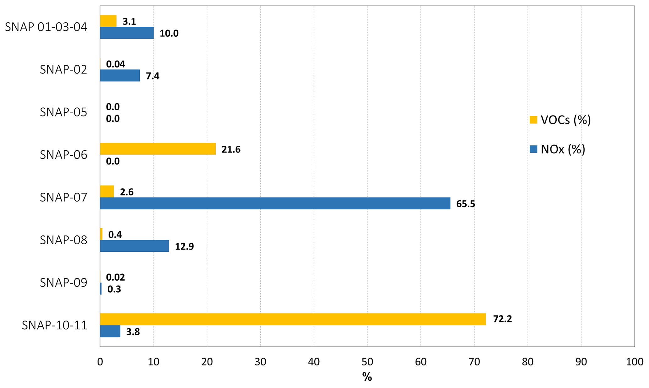
Figure 2 NO_X and VOC emissions of tagged sectors for July 2016 (percentage over total emissions in the modeling domain) for the source apportionment analysis.

In addition to the attribution of O₃ ambient levels to the emissions within the modeling domain, hereinafter referred to as local sources, the contribution of boundary conditions (BCs) and initial conditions (ICs) are estimated in this study. Considering the typical O₃ daily patterns and the variability of circulation patterns, the latter refers to the initial mixing ratios on a daily (24 h) basis, i.e., each day is run separately using the outputs from the previous day as ICs. This is different from most previous source apportionment studies that analyze shorter periods (Pay et al., 2019) or specific high concentration events (Lupaşcu et al., 2022; Zhang et al., 2022). While this may hinder the comparability of our results, this methodological option may be appropriate considering the temporal span of the period analyzed (a whole month), the typical diurnal cycle of O₃, and the goal of characterizing this attribution under specific meteorological conditions. This helps in understanding differences on O₃ source apportionment depending on regional circulation patterns (Zhang et al., 2023) and explicitly considering the influence of vertical transport of O₃ from residual layers from previous days that may lead to rapid increases in O₃ concentrations near the surface (Qu et al., 2023, and references therein). Therefore, this approach may be better suited to provide useful information for decision making, especially for the design of short-term action plans intended to control ozone peaks.

3 Results

The results are presented in four subsections. First, the main features of the simulated period and model performance are presented. Then, an overview of the source apportionment analysis carried out in the study area for the whole month is discussed. Next, this same analysis is performed for two specific days representative of different circulation patterns defined by Querol et al. (2018): advective pattern (13 July) and accumulation pattern (27 July). Additional information for 20 July and 6 July, identified by Querol et al. (2018) as advective and accumulation days, respectively, is provided in the Supplement. Finally, the temporal patterns of the O₃ apportionment are examined at the location of the air quality monitoring stations within the simulation domain. Aggregated results by station type are discussed in Sect. 3.4, while the results for different geographical areas relative to the location of Madrid city (quadrants) are presented in the Supplement.

3.1 Ozone levels during the study period and model evaluation

While this period was hotter and dryer than most of recent summers, July 2016 may be representative of typical summer conditions in the Madrid region and included a concatenation of characteristic local circulation patterns (Plaza et al., 1997) with direct implications on ground-level O₃ (Querol et al., 2018; Escudero et al., 2019). Figure 3 presents both observed and modeled concentration series at representative points (Fig. 1), and shows the venting and accumulation days identified in Querol et al. (2018). The time series demonstrate that O₃ levels are significantly lower under venting conditions, although significant differences are found depending on the location, which supports the need to use high-resolution modeling systems to analyze pollution dynamics in the Madrid region. On the other hand, accumulation patterns tend to produce higher concentrations (up to 175 µg m⁻³), especially during 27 July.

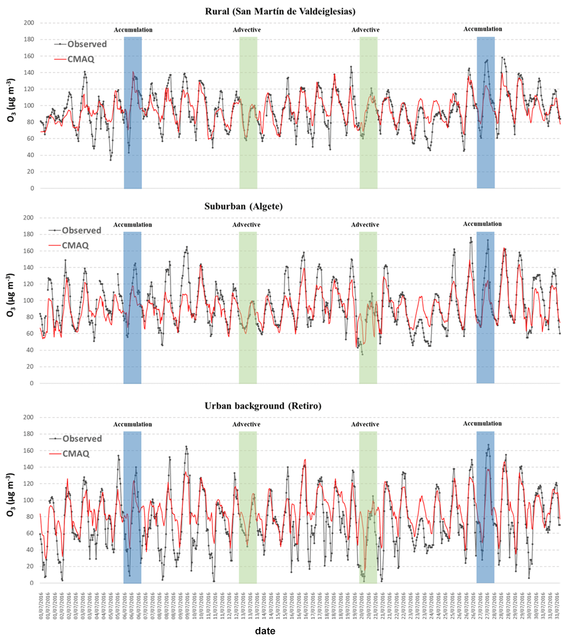
Figure 3 Observed and predicted concentration series for selected locations (1 – SMV: a rural location in the southwestern area of Madrid; 2 – ALG: a suburban location in the northeastern area of Madrid; and 3 – RET: an urban background site in Madrid's city center).

Table 2 Model performance statistics (dimensionless unless noted otherwise) by station type for ground-level O₃ concentration.​​​​​​​

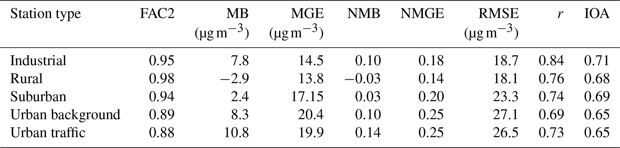
FAC2: fraction of predictions within a factor of 2; MB: mean bias; MGE: mean gross error; NMB: normalized mean bias, NMGE: normalized mean gross error; RMSE: root mean squared error; r: Pearson correlation coefficient; IOA: index of agreement.

It can be observed that the model is able to reproduce the temporal patterns, as confirmed by the high correlation coefficients (r) and index of agreement (IOA) shown in Table 2. The statistical evaluation demonstrates a reasonable model performance yielding better statistical results than recent simulation studies in this domain. Pay et al. (2019) reported an aggregated correlation coefficient of 0.66 and mean bias (MB) of 22.5 ug m⁻³ for the central region of the Iberian Peninsula. In this study, we obtained an average r value of 0.74 and an MB of 6.2 ug m⁻³. Of note, 95.2 % and 66.7 % of the r values for the locations of the 42 monitoring stations used in this study are larger than 0.6 and 0.7, respectively while the overall normalized mean bias (NMB) is only 9 %. The results for a series of common statistics (Borge et al., 2010) for each of the monitoring sites in our modeling domain can be found in Table S3. The model, however, may have some difficulties capturing the amplitude of observed O₃ series and fails to accurately reproduce concentration peaks on some days. This is evidenced by the relatively large error in comparison with the bias (23 % and 9 %, respectively, on average over the 42 monitoring stations in the modeling domain). In Table S4, we present a separate model performance assessment for accumulation and advective patterns showing that the main differences among them relate to errors, both mean gross error (MGE) and root mean squared error (RMSE), that are systematically higher for accumulation periods. This may be related to the limitations of the meteorological model in depicting atmospheric circulation during stagnation conditions suggested by Pay et al. (2019). Even when WRF was found to outperform other models for this particular episode (Escudero et al., 2019), the ability to reproduce wind direction and wind speed clearly deteriorates for accumulation periods, as shown in Table S5.

As expected, results are poorer for urban background and urban traffic locations, since the typical spatiotemporal representativeness of the measurements in such locations is not comparable with that of a mesoscale modeling system, even with 1 km² spatial resolution.

3.2 Spatial analysis of the source apportionment assessment

In this section, we discuss the contribution to ground-level O₃ of the tagged sources (Table 1) both for monthly average and high values (illustrated by the 90th percentile (P90)). O₃ apportionment focuses on anthropogenic sources since they have more interest from the point of view of possible abatement measures (Oliveira et al., 2023) and have a larger contribution than that of SNAP10-11 (below 4 % of total O₃ levels in this period). However, it is not a negligible apportionment since these groups account for 27 % (monthly mean) and 22 % (P90) of total O₃ averaged over the Madrid region when BCs and ICs are not considered (Fig. S1 in the Supplement). Non-anthropogenic emissions have been reported to play an important role in atmospheric photochemistry and they interact with man-made emissions, so they need to be considered in the process of designing policies to reduce tropospheric O₃ levels. Therefore, we discuss the potential role of emissions from agriculture and nature as well.

3.2.1 Non-anthropogenic sources

According to our results, the combined contribution of SNAP10-11 represents around 21 % and 28 % of that of local anthropogenic emissions to the monthly mean and P90. This is a similar share to that reported by Sartelet et al. (2012) at the European scale. As well as Collet et al. (2018), they argue that the influence of BVOC becomes stronger on VOC-limited areas which is consistent with our findings (Fig. S2) since the Madrid region is predominantly NO_X limited in summer, except for the metropolitan area of Madrid city and surroundings, which remain VOC limited all year-round (Jung et al., 2022, 2023). Pay et al. (2019) did not quantify explicitly the contribution of biogenic emissions to ozone in the Iberian Peninsula. However, the contribution of “other”, which included emissions from SNAP11 along with other sectors, was around 5 % in the center of the Iberian Peninsula, even though biogenic emissions represent a large fraction of total VOCs.

The contribution of BVOC to ozone levels in Europe reported by Tagaris et al. (2014), Karamchandani et al. (2017), and Zohdirad et al. (2022) are slightly larger (below 6 %) and are even more according to some source apportionment at the global scale for this latitude (Grewe et al., 2017; Butler et al., 2020). It should be noted that different experimental design and apportionment algorithms would lead to significant differences (Zhang et al., 2017; Borge et al., 2022) preventing the direct comparison of the results from different studies. In addition to the apportionment methodology itself, the results may differ depending on the emission inventory used, the modeling scale and resolution, temporal span, and sources tagging scheme. Nonetheless, the contribution of biogenic emissions found in our work is not remarkably different from that previously reported, especially for this same geographical area.

Previous studies suggested that relatively low contributions of biogenic VOCs to O₃ levels may relate to underestimations of isoprene levels (Lupaşcu et al., 2022), a very relevant species for O₃ chemistry (Dunker et al., 2016) that constitutes more than 25 % of global biogenic VOC emissions Guenther et al. (2012). Nonetheless, it is widely recognized that BVOC emission estimates involve large uncertainties (Poupkou et al., 2010; Wang et al., 2017; Zhang et al., 2017), and the MEGAN model used in this study has been found to overestimate isoprene emissions (Wang et al., 2017, and references therein). According to our inventory, isoprene represents 48 % of total BVOC. While isoprene ambient measurements are not made routinely, Querol et al. (2018) recorded an average level of isoprene around 0.2 ppb in Majadahonda, a suburban site ∼ 15 km away (in the W–NW direction) from downtown Madrid, between 5 July and 19 July 2016. That is in relatively good agreement with the results of CMAQ in our simulation, which predicted slightly less than 0.1 ppb for that location and period, as well as reproduced quite accurately the average daily pattern (see Fig. S3).

Arguably, the relatively low contribution of BVOC in our study and previous studies in this area (Valverde et al., 2016; Pay et al., 2019) may be a consequence of the underestimation of isoprene mixing ratios. However, that is compatible with the stronger influence of other anthropogenic VOC species reported elsewhere. Querol et al. (2018) estimated the total ozone formation potential (OFP) applying the maximum incremental reactivity (MIR) proposed by Carter (2009) to the VOC measurements made in their campaign for the same period and location as those in our study. Based on this methodology, they identified formaldehyde as the single most important compound (35.5 % of total OFP), while isoprene was ranked seventh with an OFP below 5 %. By family, primary BVOCs represented 6 % of total OFP on average during the experimental campaigns in this period. Similar studies elsewhere (e.g., Meng et al., 2022, in the Pearl River Delta region) have concluded as well that the ozone formation potential of BVOCs is lower than that of anthropogenic VOCs applying a similar reactivity scale (Carter and Atkinson, 1989). That may be consistent with the apparent insensitivity of O₃ to isoprene emissions reported in other studies (Simpson, 1995; Jiang et al., 2019; Ciccioli et al., 2023).

Of note, SNAP10-11 include NO_X emissions from soils (see Sect. 2.4). Although they represent less than 4 % of total NO_X emissions in the domain, they may be underestimated by MEGAN (Visser et al., 2019). According to other studies, for example, Weng et al. (2020), emissions from agricultural soils may be substantially higher and could pose a significant constraint in the control of O₃ levels (Lu et al., 2021). Methods to reduce the uncertainty in NO_X emissions estimates from soils as well as their role in O₃ control policies specifically for this region may be addressed in future research.

Other non-controllable sources include stratospheric ozone, also tagged in this study (ST in Fig. 12). This source informs about the influence of vertical injections on ground-level O₃ levels (Hsu et al., 2005) and the potential contribution reported in this region for specific extraordinary ozone levels (San José et al., 2005). Pay et al. (2019) hypothesize that stratosphere–troposphere exchange (STE) may have played a significant role towards the end of July 2016 in the Iberian Peninsula. According to our results, however, the direct transport of O₃ from the stratosphere in our modeling domain was negligible in this period, with 1 h maximum contributions below 0.4 ppb in the southwest end of the Madrid region (see Fig. S4). This contrasts with remarkably higher contributions reported in other areas of Europe (Lupaşcu et al., 2022) and those from global simulations for similar latitudes (Butler et al., 2018). It should be noted that here we account for O₃ STE exclusively within our innermost nested domain and part of the O₃ attributed to BCs may be related to contributions from the stratosphere in other regions.

3.2.2 Anthropogenic sources

Figure 4 shows the contribution to ground-level O₃ of the BCs and that of all local anthropogenic emissions combined for both monthly average and high values (illustrated by the 90th percentile (P90)). In both cases BCs are the largest contributor. This is consistent with previous studies that have identified boundary conditions as the dominant contribution to ground-level O₃, e.g., Pay et al. (2019) for the Iberian Peninsula, Collet et al. (2018) for the USA, or de la Paz et al. (2020) for Madrid specifically. However, the weight of each of the sources on both metrics is different. On average, 70 % of the mean O₃ levels in the Madrid region comes from BCs (Fig. 4a), while for P90, the contribution from BCs is considerably smaller, around 50 % (Fig. 4b).

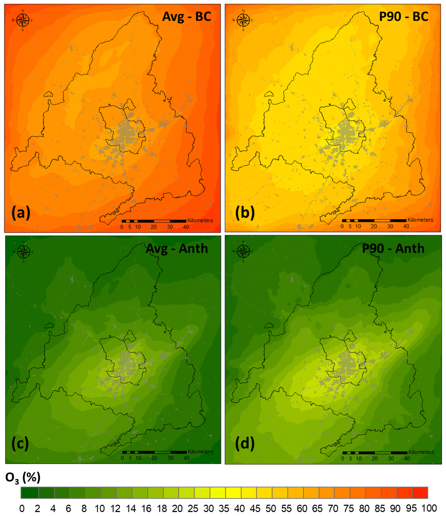
Figure 4 Contribution (%) of BCs to O₃ concentration: (a) monthly average and (b) 90th percentile. Contribution (%) of local anthropogenic emissions to (c) monthly average and (d) 90th percentile.

The maximum anthropogenic contribution for the monthly average (Fig. 4c) reaches 17 % (7.5 ppb in absolute terms), with a mean contribution of 8.7 % over the whole Madrid region (Fig. S1). Regarding P90 (Fig. 4d), the maximum contribution of local anthropogenic emissions is 28 % (in the center and southwest of the Madrid municipality), around 22 ppb in absolute terms. This corresponds to a spatially averaged contribution of 12.2 % over the Madrid region (Fig. S1), which corresponds to an absolute value around 11 ppb. Despite the general dominance of BCs on O₃ levels, these results point out that the relevance of local emissions (Fig. 2) is higher for O₃ peaks, a finding consistent with those of previous studies (Valverde et al., 2016; Qu et al., 2023).

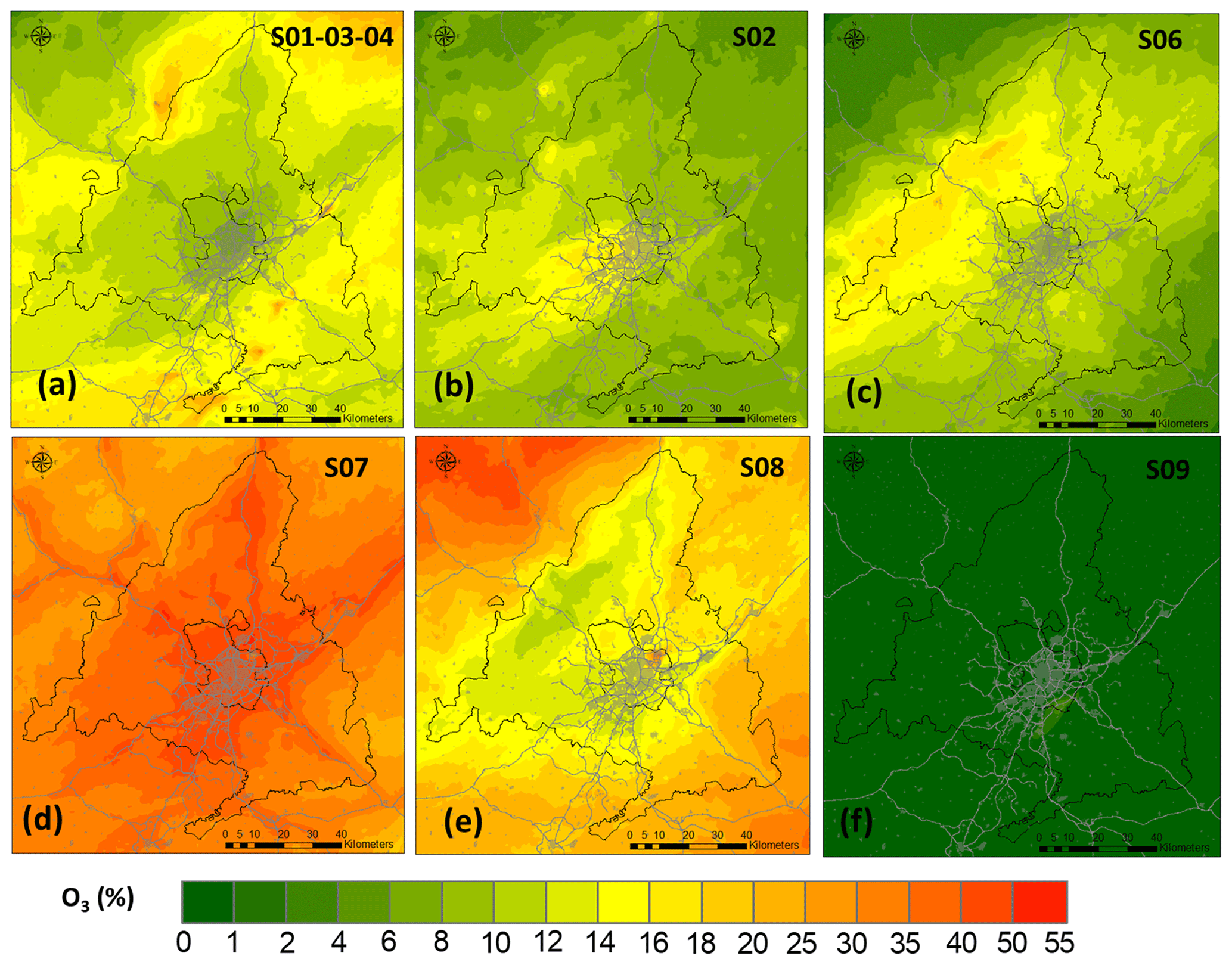
Figure 5 Percentage contribution to the 1 h O₃ 90th percentile of the main emitting sectors with respect to the total anthropogenic contribution.

Figure 5 shows the apportionment to P90 of each emission sector for local sources. Consistent with Valverde et al. (2016) and Pay et al. (2019), our results clearly identify road transport (SNAP 07) as the most influential sector, contributing 41 % to P90 on average over the Madrid region. The contribution of this sector (relative to local sources) reaches values up to 55 % in the proximity of the main communication routes (Fig. 5d). In absolute terms, this means an average contribution of 5 ppb and a maximum one of 11 ppb (Fig. S5). The next sector with the highest contribution relates to off-road mobile sources (SNAP08), with an average contribution in the Madrid region of 17 % (1.8 ppb) and a maximum of 8 ppb in the vicinity of the Adolfo Suárez Madrid–Barajas airport. This suggests that NO_X emissions play a more important role than VOC emissions in the photochemical production of ozone, in concurrence with previous source apportionment studies (Dunker et al., 2016; Butler et al., 2018; de la Paz et al., 2020). Nonetheless, the importance of controlling anthropogenic VOC emissions to prevent high-O₃ episodes has been noted in previous studies (Cao et al., 2022), even in regions with strong biogenic emissions (Coggon et al., 2021). In addition to the contribution of BVOC previously discussed, anthropogenic VOC had also an influence on O₃ levels during July 2016 in the Madrid region (see Fig. S2). While the spatially averaged attribution of SNAP06 to P90 is only 1.5 ppb with maximum contributions of 3 ppb at specific locations (southwest of Madrid as shown in Figs. S2 and S5), emissions from the use of solvents and other products can reach values up to 20 % of total anthropogenic contributions to O₃ P90 (Fig. 5c). This is comparable to the contribution of all industrial sources combined (SNAP01-03-04). This may be related to the high OFP of aromatics within SNAP06 VOC (Meng et al., 2022) and is consistent with the findings of Oliveira et al. (2023) that attributed 64 % of total OFP to the solvent sector (relative to that of total anthropogenic VOC) in densely urbanized areas such as Madrid. Coggon et al. (2021) also found that consumer and industrial products (included in SNAP06 group) are important precursors of ozone in urban areas, which typically present a VOC-sensitive regime. Nonetheless, they found that O₃ formation may take a few hours and the maximum contributions of VOC emitted in New York City occur a few tens of kilometers away, close to NO_X-limited areas. Our high-resolution analysis indicates that a similar process may take place in Madrid too. The rest of the sectors analyzed (SNAP05 and SNAP09) have negligible contributions (around 0.05 ppb on average over the Madrid region).

If the analysis is done on a daily basis, it is worth noting the significance of the initial conditions (ICs) as well, with a spatially averaged contribution of 19 % and 34 % to the monthly average and P90 O₃ levels, respectively (Fig. S1). However, the role of ICs is more relevant in analyzing how meteorological conditions may affect source apportionment. Of note, in this study “ICs” refers to O₃ from the previous 24 h period. Consequently, the effect of ICs on O₃ does not necessarily diminish throughout the month. Instead, we found that the influence of ICs relates mainly to regional circulation patterns. We elaborate on this in the following sections.

3.3 Source apportionment assessment under characteristic circulation patterns

The study of the influence of meteorology on the O₃ ambient levels is carried out by analyzing the results for specific days representative of the two circulation patterns. Querol et al. (2018) identified an advective pattern for 13 and 20 July and an accumulation pattern for 6 and 27 July. In this section, we examine the source apportionment for those days (days 13 and 27 in more detail) to test the hypothesis that local atmospheric conditions may induce a significant difference in O₃ attributions, as reported elsewhere (Zhang et al., 2023).

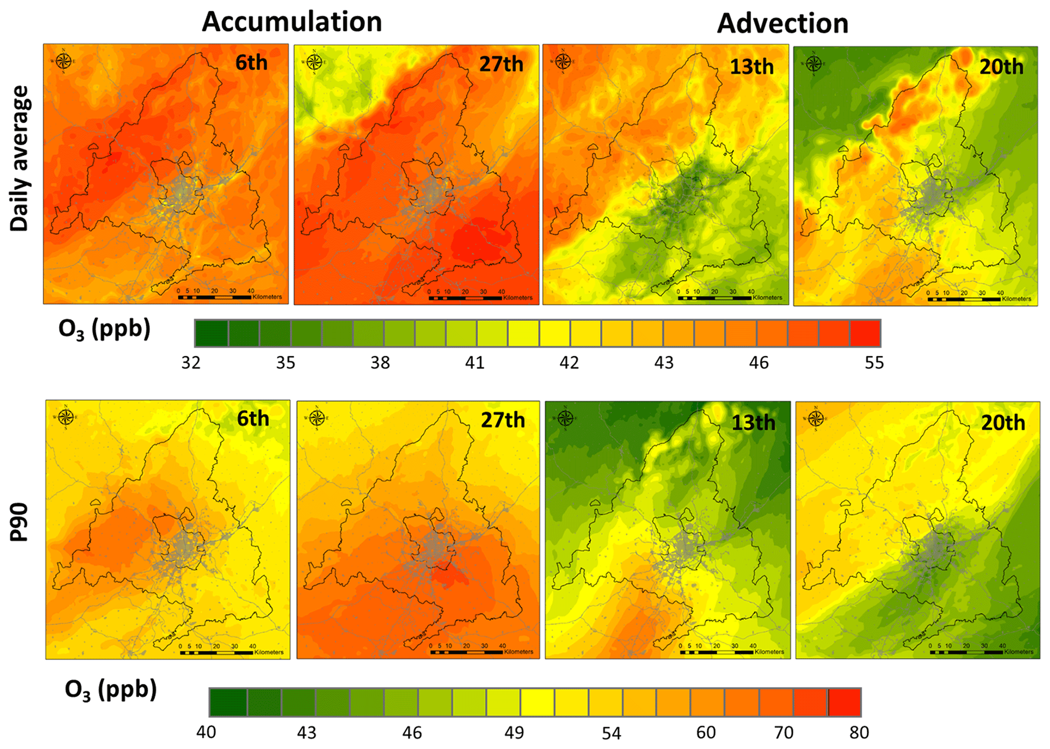
Figure 6 Daily mean (top) and 90th percentile (bottom) of O₃ levels (ppb) during accumulation (6 and 27 July 2016) and advective (13 and 20 July 2016) periods.

Figure 6 shows the daily average and the P90 of hourly O₃ levels during the accumulation and advective episodes. It is observed that during accumulation days (days 6 and 27), mixing ratios averaged over the Madrid region were 13 %–20 % higher than those of advective periods (days 13 and 20) and, although not shown, around 4 %–8 % higher than the monthly average. Regarding the maxima, the average P90 (third highest hourly mixing ratio for a given day) during the accumulation periods in the Madrid region may be 25 % higher than that of the ventilation periods.

3.3.1 Accumulation pattern

Consistent with previous studies that highlight the impact of meteorological conditions on O₃ (Nguyen et al., 2022), modeling results show that accumulation days are especially relevant regarding the potential impacts on health and vegetation, and a deeper analysis of pollution dynamics under those conditions is of interest. Figure 7 shows the hourly evolution (03:00, 09:00; 15:00, 21:00 UTC) of surface O₃ mixing ratios during the day 27 (day 6 is shown in Fig. S7), along with O₃, NO_X, and VOC vertical levels up to 5 km height for a NE–SW cross section, related to the dominant wind directions. (The same results for a perpendicular SE–NW cross section are shown in Fig. S8.)

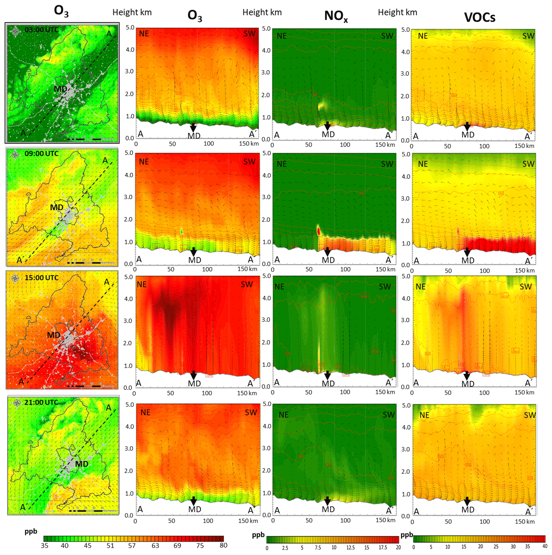
Figure 7 Accumulation period: evolution during 27 July 2016. From left to right: plan view and NE–SW cross section (up to 5 km height) O₃ mixing ratios (ppb), NO_X (ppb), and VOCs (ppb) at the 03:00, 09:00; 15:00, 21:00 UTC hours. MD: Madrid city.

A low O₃ mixing ratio surface layer (around 40 ppb) can be clearly seen for the early hours of the day (03:00 UTC, 05:00 LT). This relates to a shallow planetary boundary layer (PBL) (a few hundred meters high) and weak winds (1–2 m s⁻¹) from the NE. Around 06:00 UTC (08:00 LT), the main emitting sectors (such as road transport) begin to emit O₃ precursors (see Quaassdorff et al., 2016) for characteristic emission temporal profiles. The prevailing surface wind directs the urban plume towards the SW and the southern slope of the Sierra de Guadarrama (Fig. S6). Of note, the wind direction aloft is the opposite, in accordance with recirculation processes reported for this domain (Plaza et al., 1997). As the day progresses (09:00 UTC, 11:00 LT), the PBL height grows (up to 1.5 km) as radiation and temperature increase, mixing O₃ vertically. At the same time, the emissions of precursors (concentrated in Madrid city) lead to an increase in the local production of O₃ in the plume, more evidently in the rural areas (NO_X-limited regions) in the leeward side of the city. On the contrary, in the vicinity of high NO_X emission intensity areas, O₃ is consumed by NO through the reaction $\mathrm{NO}+{\mathrm{O}}_{\mathrm{3}}\to {\mathrm{NO}}_{\mathrm{2}}+{\mathrm{O}}_{\mathrm{2}}$, a titration effect documented in previous studies (Saiz-Lopez et at., 2017).

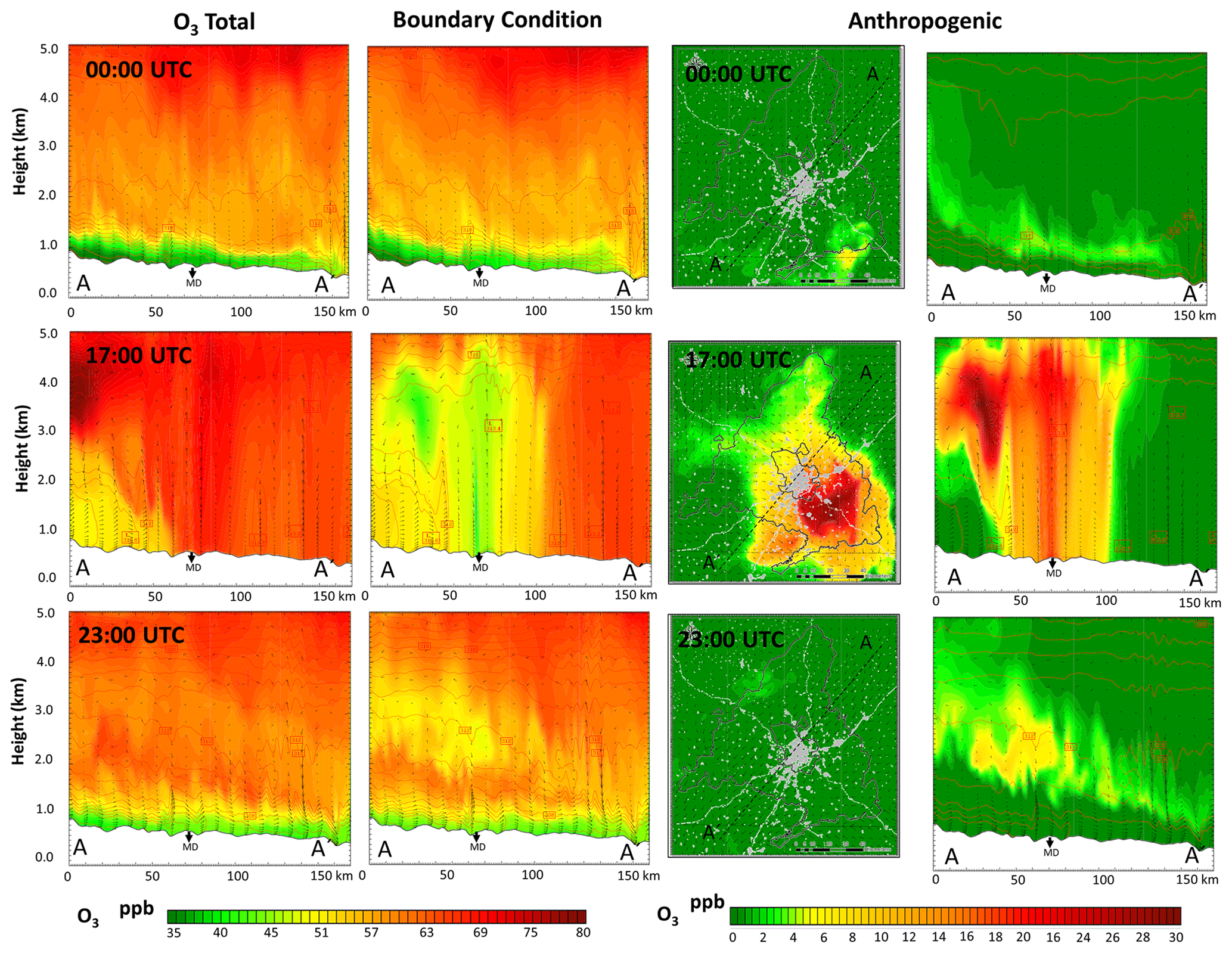
Figure 8 Hourly O₃ mixing ratio profiles (at 00:00, 17:00; 23:00 UTC) for the NE–SW cross section as well as the contribution of BCs and anthropogenic local emissions on 27 July 2016 (accumulation). MD: Madrid city.

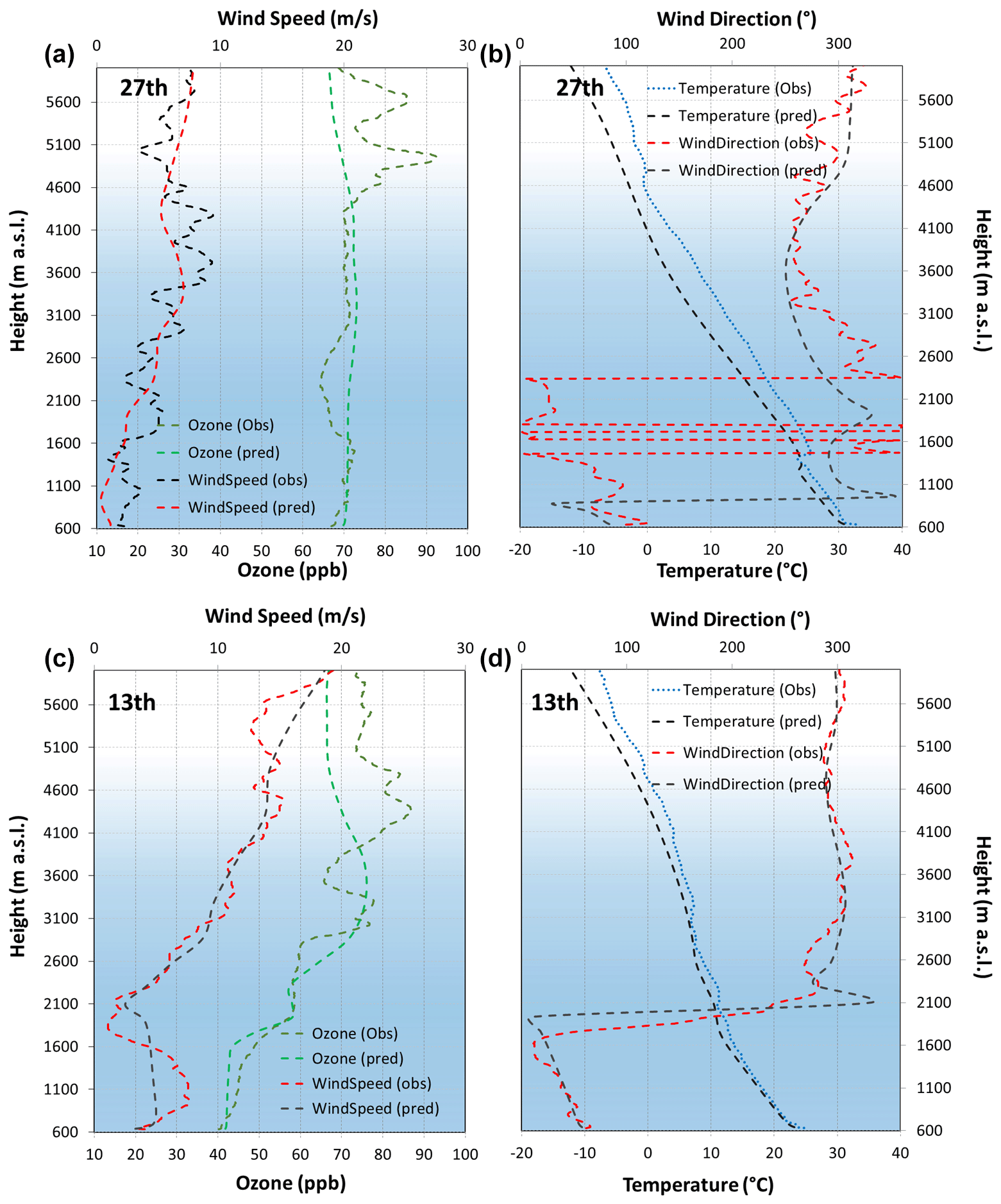
Figure 9 Vertical profiles (12:00 UTC) of O₃ mixing ratios, temperature, wind speed, and wind direction for 27 July (accumulation, up) and 13 July (advective, down).

Over the following midday hours (09:00–15:00 UTC, 11:00–17:00 LT) the PBL further develops and a vertical homogenization process occurs. There is a deep vertical mixing of newly formed ozone with O₃-enriched upper layers generated in previous days (Querol et al., 2018; Escudero et al., 2019). As illustrated in Fig. 8, there is a first O₃ reservoir located around 1500 m altitude (at 00:00 UTC, 02:00 LT) that relates mainly to local sources and contributes with 2–8 ppb, while higher O₃ reservoirs (around 4000 m a.s.l.) relate to BCs and have a considerably higher contribution (50–75 ppb). Around 15:00 UTC (17:00 LT) the PBL reaches 3000–4000 m in accumulation periods and O₃ levels up to 75–80 ppb are found (Fig. 7). This dynamic is compatible with the ozone sounding (https://woudc.org/data/explore.php; last access: 10 November 2022) included in Fig. 9, which shows a very constant O₃ value around 65–70 ppb from the surface to 4000 m a.s.l.

Later, around 17:00 UTC, the local O₃ production from anthropogenic local emissions released earlier is the maximum (Fig. 8), with ground-level contributions that can reach 30 ppb SE in the municipality of Madrid. However, the greatest contribution during these hours continues to be from the BCs (up to 50–60 ppb at surface level). From 21:00 UTC, the PBL has already decreased to a few hundred meters, the turbulence dwindles, the surface flow towards the SW is re-established, and the formation of enriched levels of precursors (Fig. 7) and ozone (Fig. 8) in the 1000–2000 m a.s.l. occurs again, in accordance with the regional recirculation processes reported in the literature for this area (Querol et al., 2018; Escudero et al., 2019).

3.3.2 Advective pattern

As an example of an advective pattern, Fig. 10 shows the plan view and the NE–SW cross section of O₃, NO_X, and VOC levels during 13 July. (Figure S9 shows the SE–NW cross section for day 13, and Figs. S10 and S11 represent the NE–SW cross section and the SE–NW cross section for day 20, respectively.) It can be seen that surface O₃ levels at 03:00 UTC are around 8 % lower than those of 27 July (accumulation) (in the Madrid region average of 39 and 42 ppb for advective and accumulation conditions, respectively) with maximum values along the Sierra de Guadarrama, where elevated terrain reaches layers rich in O₃ and precursors from the lower troposphere and from the residual layers formed the day before (Fig. S11). This occurs (also under accumulation conditions) when the PBL height is lower than the maximum height of the Sierra de Guadarrama. However, during advective periods, a stronger stratification of O₃ is observed during the early hours (03:00–09:00 UTC) due to the existence of more intense wind direction speed vertical gradients (relative to accumulation conditions), perfectly captured by the modeling system (Fig. 11).

Figure 10 Advective period: hourly evolution during 13 July 2016. From left to right: plan view and NE–SW cross section (up to 5 km height) O₃ mixing ratios (ppb), NO_X (ppb), and VOCs (ppb) at the 03:00, 09:00; 15:00, 21:00 UTC hours. MD: Madrid city.

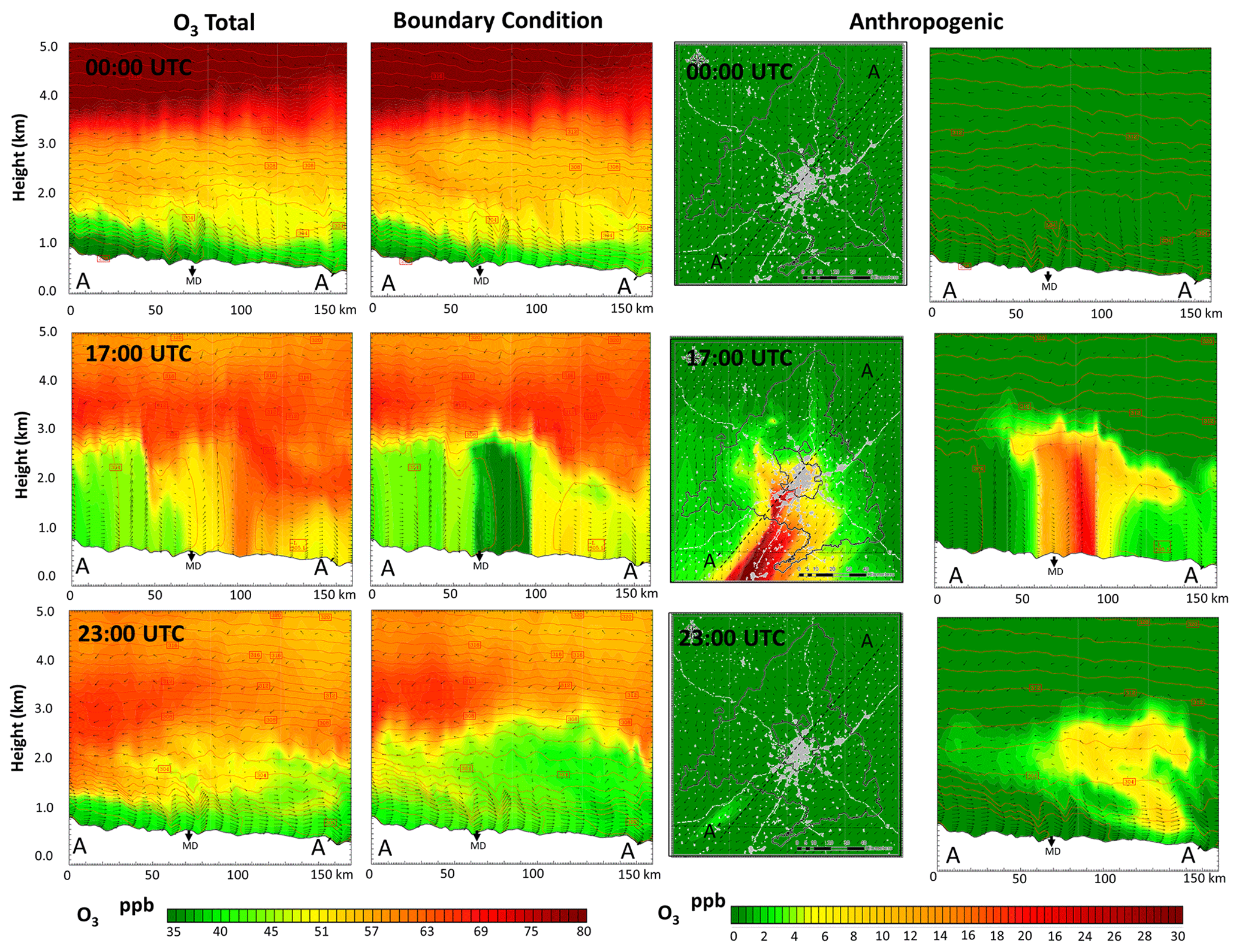
Figure 11 Hourly O₃ mixing ratios (at 00:00, 17:00; 23:00 UTC) for the NE–SW cross section as well as the contribution of BCs and anthropogenic local emissions on 13 July 2016 (advection). MD = Madrid city.

At 09:00 UTC, the local O₃ production downwind of the city is lower than during the accumulation periods (Fig. S12), not only quantitatively but also in terms of the total area affected. This can be explained by the weather conditions (promoting dispersion) and the corresponding lower surface levels of the main precursors (5–8 ppb NO_X and 15–20 ppb of VOCs on the day 13, compared with 10–15 ppb NO_X and 30–40 ppb of VOCs during accumulation on day 27). At 15:00 UTC (Fig. 10), the PBL height increases reaching 2500–2800 m altitude (compared with 4000 m on day 27). As the PBL grows, the vertical mixing dominates the wind-driven pollution displacement in the SW direction. Similarly to the dynamics described for accumulation conditions, this allows precursors and fresh O₃ to ascend and mix existing ozone in higher layers (Figs. 10 and 11). Nonetheless, the vertical mixing is lower during advective patterns, as observed in the ozone soundings (Fig. 9), with the consequent difficulty of the boundary layer to incorporate O₃ from higher strata (beyond 4000 m a.s.l.) in the central hours of the day. This results in lower O₃ mixing ratios at surface level under advective conditions, up to 60 ppb SW of Madrid city (Fig. 10). As for the relative importance of local sources, Fig. 11 shows that their contribution can reach nearly 30 ppb, similar to that under accumulation conditions. However, the area affected is clearly associated with the city plume and their contribution averaged over the region is smaller. In fact, our results point out that precursors advected can produce hourly peaks above 30 ppb outside the Madrid region.

3.4 Source apportionment assessment at the location of monitoring stations

A source apportionment assessment has also been carried out at the location of the air quality monitoring stations distributed throughout the simulation domain (Fig. 1) to inform on the contributions of different sources at those points where air quality is routinely monitored. Differences are found depending on the type of station (urban, suburban, or rural) and, consistent with the results discussed in the previous subsection, the type of circulation pattern (advective or accumulation). The results are summarized in Fig. 12. As previously discussed, it shows the contribution of all anthropogenic emission sources (S01-03-04 to S08), biogenic emissions (SNAP10-11) as well as boundary and initial conditions (BCs and ICs), and O₃ stratospheric transport (ST). Although 100 % of emitting sectors have been tagged, Fig. 12 shows as well the contribution from “others” (OTH). This contribution is typically negligible and relates to minor model interactions between sources and species not considered by the ISAM model. Details are fully explained in the documents provided with the model release (US EPA, 2022).

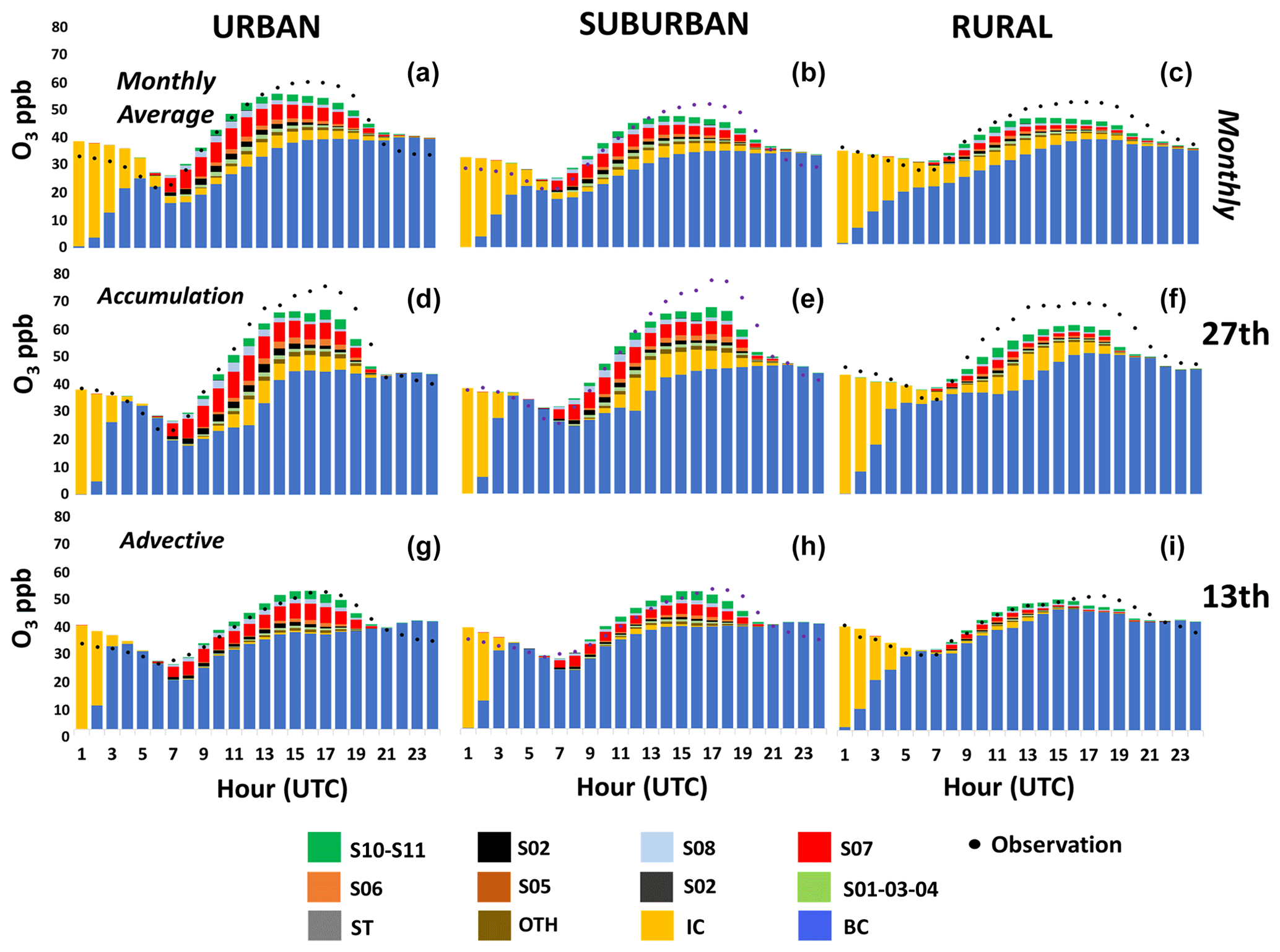
Figure 12 Hourly contribution to ground-level O₃ for the monthly average (a–c) and specifically for accumulation (27 July 2016) and advective (13 July 2016) days (d–f and g–i, respectively).

Urban and suburban monitoring stations have a similar aggregated behavior. During the first hours of the morning, the initial and boundary conditions make up the totality of O₃ levels until 06:00 UTC approximately. After that time, O₃ generated from precursors emitted by local sources appears, reaching contributions up to 15 and 12 ppb for urban and suburban locations (28 % and 22 % of the total ozone, respectively) around 12:00 UTC. The road transport (14 %–10 %) and the residential (2 %–4 %) sectors are those with the highest contributions. The signal of anthropogenic sources is lower in rural monitoring stations. On average, road traffic contributes a maximum of 5 % (5 ppb), the residential sector 2 % (2 ppb), and the use of solvents (VOC emissions) also around 2 % in rural locations.

The results in Fig. 12 demonstrate the persistent relevance of ICs at all locations, but especially in rural locations. Even though the initial conditions contribute to O₃ levels throughout the day, the maximum values are found in the first hours (00:00–05:00 UTC). As the day evolves, the influence of ICs progressively decreases until they disappear at 21:00 UTC approximately. However, clear differences are found depending on the circulation pattern as illustrated for 27 July (accumulation) and 13 July (advection). According to the model predictions, O₃ levels are greater during the accumulation period (and are reached slightly earlier), with maxima up to 68 ppb (17:00 UTC) in contrast with 52 ppb under advective conditions. Of note, the model reproduces observed O₃ temporal patterns quite consistently, but it misses the peak values during accumulation periods, as discussed in Sect. 3.1.

It can be highlighted that the influence of residual layers of the previous day, tracked through the IC tag and observed again during the central hours of the day, is very significant under accumulation conditions (IC contribution of up to 12 ppb, around 18 % of total O₃), while it is practically missing for advective days. This relates to the enhancement of O₃ levels from reservoirs aloft, discussed in Sect. 3.3.1, that does not occur under advective conditions. Of note, and consistent with the analysis in Sect. 3.3, we observe that the average contribution from local anthropogenic sources to O₃ peaks (around 16:00 LT) in urban locations in accumulation periods is higher than that of advective periods. That is true both for absolute levels (18 and 11 ppb, respectively) and relative contributions (32 % and 22 %, respectively). These results point out that the source apportionment under unfavorable circulation patterns significantly differs from that for average or advective conditions and, consistent with previous studies (Lupaşcu et al., 2022; Qu et al., 2023), demonstrate that the influence of local sources is larger for high O₃ levels under stagnation conditions.

Nonetheless, clear differences are found for individual stations depending on their location relative to the city center and prevailing winds. In the Supplement (Figs. S14–S16) a stratification of the same results by station type and geographical quadrant (Fig. S13), as well as distance to Madrid, is shown. For instance, urban locations within Madrid municipality in the NE direction for 27 July (accumulation) present much higher contributions from local sources than those of urban stations in the NW direction and further away from the metropolitan area (Fig. S15). This variability suggests that the outcome of local measures may differ throughout the region and should be modeled under specific meteorological conditions and assessed specifically for each location of interest.

4 Conclusions

A high-resolution chemical-transport model has been used to investigate O₃ dynamics for a typical summer month (July 2016) in the Madrid region. The model presents an acceptable performance and succeeds in reproducing the phenomena described in previous studies (Querol et al., 2018; Escudero et al., 2019), confirming that O₃ dynamics are conditioned by regional circulation patterns. Nonetheless, we found that model errors are larger for accumulation days and concentration peaks are underestimated. This may be related to an inadequate performance of the meteorological model under stagnation conditions. A novel implementation of CMAQ-ISAM (Shu et al., 2023) that attributes O₃-based reaction stoichiometry with all production and destruction reactions involved has been applied to perform a source apportionment of this non-linear, secondary pollutant under specific weather patterns. Our simulation shows that O₃ levels are dominated by non-local contributions (i.e., boundary conditions), representing around 70 % of mean values across the region. Ozone reservoirs from previous days (labeled as initial conditions in our methodology) in the mid troposphere are also important to build up high O₃ levels in accumulation episodes, representing the main difference with advective periods. The analysis, however, points out that precursors emitted by local sources play a more important role regarding the highest mixing ratio values, illustrated in this study by the 90th percentile. This suggests that the implementation of emission reduction strategies in the region may be more effective to control O₃ peaks than average values. This is particularly true under unfavorable, stagnation conditions associated with accumulation patterns when the highest O₃ values occur. According to our results, up to 35 % of total O₃ may originate from local sources, giving a theoretical maximum reduction potential of 1 h values of approximately 25 ppb under these conditions. Among local sources, road traffic is the main contributor, accounting for 55 % of local sources. Our results suggest that NO_X emissions play a more important role than VOC emissions in the photochemical production of ozone. Nonetheless, we found that the use of solvents and other products, a significant source of VOC emissions with high ozone formation potential, can explain up to 20 % of the O₃ originating from local anthropogenic emissions in some locations. At the same time, our results point out that the contribution of biogenic emissions is lower than that of anthropogenic sources (below 4 % of total O₃ levels in this period), although they are responsible for 42.4 % of total VOCs in the modeling domain. Emissions from other sectors play a minor role and O₃ transported from the stratosphere within the model domain is negligible.

We also found significant variations in source apportionment patterns across station types and locations. This implies that high-resolution simulations under specific meteorological conditions should be performed to anticipate the potential outcome on O₃ levels in different locations of the Madrid region.

Considering these results, future modeling efforts should be oriented to simulate the effect of specific measures, both locally and in cooperation with other administrations, to identify optimal emission abatement strategies. The modeling platform used in this study may be also helpful in assessing sensitivities to different factors, including photochemical regimes or NO_X and VOC speciation for specific sources. Furthermore, the role of biogenic NO_X and VOC emissions may be further studied to understand the implications of O₃ control strategies in the Madrid region.