The Antarctic stratospheric nitrogen hole: Southern Hemisphere and Antarctic springtime total nitrogen dioxide and total ozone variability as observed by Sentinel-5p TROPOMI

Denitrification within the stratospheric vortex is a crucial process for Antarctic ozone hole formation, resulting in an analogous stratospheric “nitrogen hole”. Sedimentation of large nitric acid trihydrate polar stratospheric cloud particles within the Antarctic polar stratospheric vortex that form during winter depletes the inner vortex of nitrogen oxides. Here, 2018–2021 daily TROPOspheric Monitoring Instrument (TROPOMI) measurements are used for the first time for a detailed characterization of this nitrogen hole. Nitrogen dioxide total columns exhibit strong spatiotemporal and seasonal variations associated with photochemistry as well as transport and mixing processes. Combined with total ozone column data two main regimes are identified: inner-vortex ozone- and nitrogen-dioxide-depleted air and outer-vortex air enhanced in ozone and nitrogen dioxide. Within the vortex total ozone and total stratospheric nitrogen dioxide are strongly correlated, which is much less evident outside of the vortex. Connecting the two main regimes is a third regime of coherent patterns in the total nitrogen dioxide column–total ozone column phase space – defined here as “mixing lines”. These mixing lines exist because of differences in three-dimensional variations of nitrogen dioxide and ozone, thereby providing information about vortex dynamics and cross-vortex edge mixing. On the other hand, interannual variability of nitrogen dioxide–total ozone characteristics is rather small except in 2019 when the vortex was unusually unstable. Overall, the results show that daily stratospheric nitrogen dioxide column satellite measurements provide an innovative means for characterizing polar stratospheric denitrification processes, vortex dynamics, and long-term monitoring of Antarctic ozone hole conditions.

1 Introduction

Stratospheric nitrogen plays a crucial role in catalytic polar stratospheric ozone depletion. That occurs when halogens – mostly chlorine but also some bromine – are massively released from stable reservoir species like ClONO₂, HOCl, and HCl (Solomon, 1990; Solomon and Keys, 1992; Dessler, 2000; von Clarmann, 2013). Extremely low stratospheric temperatures during polar winter and the development of the stratospheric polar vortex result in widespread formation of small particles containing nitrogen oxides – forming so-called polar stratospheric clouds (PSCs) – which slowly sediment. This process – called denitrification or denoxification – depletes nitrogen oxides in the polar stratospheric vortex (Farman et al., 1985; Solomon and Garcia, 1983; Salawitch et al., 1989; Fahey et al., 1990; Tabazadeh et al., 2000; Weimer et al., 2023). Strong zonal winds at the stratospheric polar vortex edge prevent resupply of nitrogen oxides from outside the vortex. The return of sunlight to the polar stratosphere during polar spring to the denitrified polar stratosphere leads to the formation of halogen radicals (Solomon, 1999​​​​​​​; Santee et al., 2008; Strahan et al., 2014). The lack of nitrogen oxides – combined with the presence of PSCs – allows the halogen radicals to catalytically destroy ozone. This process causes the rapid formation of the well-known Antarctic ozone hole (Hurwitz et al., 2015). Polar stratospheric ozone depletion ceases when either all ozone is destroyed or the stratosphere becomes warm enough and unfavorable for PSCs while being favorable again for stable halogen reservoir species like HCl (Müller et al., 2008; Strahan et al., 2019; Stone et al., 2021). The warming in turn is caused by increasing sunlight and absorption of that sunlight but sometimes also by increased planetary wave activity (de Laat and van Weele, 2011; Wargan et al., 2020; Smale et al., 2021).

The ozone-depleted Antarctic stratospheric vortex (“ozone hole”) is easily identified in, for example, satellite measurements of the total ozone column (TCO₃). It is characterized by a large gradient of ozone-rich outer-vortex air and O₃-depleted inner-vortex air. This gradient is not only present in O₃ but also in other trace gases like nitrogen oxides, as outlined and pioneered by John F. Noxon in the late 1970s (Noxon, 1978, 1979). This cliff-like large vortex-edge trace gas gradient (Schoeberl et a., 1992; Joseph and Legras, 2002; Waugh and Polvani, 2010) is therefore referred to as the “the Noxon cliff”. The presence of this cliff reflects air masses on either side of the cliff with very different chemical histories (Dirksen et al., 2011).

Studying Noxon cliff characteristics for a long time depended on numerical modeling (e.g., Solomon and Garcia, 1983; Toon et al., 1989; Garcia and Solomon, 1994; Struthers et al., 2004), ground-based observations (e.g., Gil and Cacho, 1992; Solomon et al., 1993; Kondo et al., 1994; Sanders et al., 1999; Struthers et al., 2004; Bortoli et al., 2005; Yela et al., 2005; Cook and Roscoe, 2009), and aircraft or balloon measurement campaigns over Antarctica (e.g., Goldman et al., 1978; Pommereau and Goutail, 1988; Fahey et al., 1989).

The advance of new innovative satellite instruments from the middle 1990s onwards, but especially after 2000, has enabled exploration of new approaches for monitoring the Antarctic Noxon cliff (Bodeker et al., 2002; Ricaud et al., 2005; Manney et al., 2005; Sato et al., 2009). The use of satellite observations for studying polar stratospheric nitrogen compounds and the Noxon cliff has been predominantly done with satellite limb observations (e.g., Callis et al., 1983; Mount et al., 1984; Rinsland et al., 1996; Haley et al., 2004; Funke et al., 2005; von Savigny et al., 2005; Butz et al., 2006; Davies et al., 2006; Kerzenmacher et al., 2008; Kühl et al., 2008; Kritten et al., 2010; Bourassa et al., 2011; Khosrawi et al., 2011; Sofieva et al., 2012; Belmonte Rivas et al., 2014; Khosrawi et al., 2017; Dubé et al., 2020; Strode et al., 2022; Russell et al., 1984). Note that many of these papers only touch upon the Noxon cliff; i.e., it is seen in the measurements and presented as an example of the observational capacity of a certain satellite and/or data product. Some results have been reported on the use of nitrogen dioxide (NO₂) total columns and/or stratospheric columns for nadir-looking satellites but without a focus on polar regions (Belmonte Rivas et al., 2014; Beirle et al., 2016). Note that a main interest in stratospheric or total NO₂ from nadir-viewing satellites is because of the need to remove the stratospheric component from total column amounts to arrive at the tropospheric NO₂ column (e.g., Hilboll et al., 2013).

There are a few research publications that touch upon satellite nadir total or stratospheric nitrogen dioxide (NO₂) observations over polar regions. Wenig et al. (2004) explore satellite nadir total stratospheric NO₂ (SNO₂) column measurements from the Global Ozone Monitoring Experiment (GOME). They identify the Noxon cliff in Arctic springtime observations in 1997 in relation to the Arctic stratospheric vortex, which persisted much longer than typical during that year. However, they do not explore the Antarctic region for similar purposes even though they mention multiple times that the Noxon cliff is present in both polar regions and that denitrification is larger over Antarctica relative to the Arctic. Richter et al. (2005) also explore GOME observations of total column O₃ (TCO₃), total NO₂ (TNO₂), and OClO over Antarctica during the early 2000s with a focus on the well-known September 2002 Antarctic vortex split​​​​​​​ (Ricaud et al., 2005; Richter et al., 2005; von Savigny et al., 2005; Yela et al., 2005). They observe strongly reduced inner-vortex SNO₂ during early Antarctic spring that largely vanished after the vortex split. However, no effort has been put into quantitatively correlating TNO₂ $/$ SNO₂ with TCO₃ and/or OClO. Adams et al. (2013) explore some Ozone Monitoring Instrument (OMI) TNO₂ data and TCO₃ data in their study of ground-based observations at the Eureka station in northern Canada in relation to the anomalous longevity of the 2011 Arctic stratospheric vortex. They observe enhanced NO₂ and O₃ when outer-vortex air passes over Eureka associated with photochemical NO₂ production and the stratospheric vortex preventing mixing of outer-vortex air with inner-vortex air, causing NO₂- and O₃-rich stratospheric air to accumulate in the region bordering the Antarctic stratospheric vortex. They also show the conjunction of NO₂- and O₃-depleted inner-vortex air in OMI data. Gordon et al. (2020) explore OMI TNO₂ and TCO₃ in relation to (upper-)stratospheric and mesospheric NO_x formation due to energetic particle precipitation (EEP) but do not explore OMI TNO₂ beyond that application. The Noxon cliff has also been identified in satellite nadir observations of nitrous acid (HNO₃) total columns from the European Infrared Atmospheric Sounding Interferometer (IASI) satellite (Wespes et al., 2009, 2022; Ronsmans et al., 2016) as removal of HNO₃ from the Antarctic stratosphere is the main denitrification process. Those studies showed that – not unexpectedly – Antarctic stratospheric vortex stability was important for inner-vortex HNO₃ and the strength of the Noxon cliff. However, in-depth analysis of the Noxon cliff in IASI HNO₃ observations is also still lacking. Note that strong cross-vortex gradients have also been observed in nadir-viewing satellite measurements of OClO (Kühl et al., 2006, 2008; Oetjen et al., 2011; Puķīte et al., 2021; Pinardi et al., 2022).

Satellite-observation-based exploration of the Noxon cliff and the denitrification process has thus almost exclusively been restricted to limb-sounding types of satellites. Insofar as can be assessed the use of satellite nadir NO₂ measurements for in-depth study of the Antarctic stratosphere and denitrification has been absent. Even exploitation of the IASI HNO₃ data for this purpose has remained limited – in part also because of the need to average IASI HNO₃ data to reach sufficient data accuracy.

The TROPOspheric Monitoring Instrument (TROPOMI) is the first of the next generation of hyperspectral UV–VIS satellite instruments. Designed and developed based on experience with satellite instruments like GOME, SCIAMACHY (SCanning Imaging Absorption spectroMeter for Atmospheric CHartographY), GOME, and GOME-2 it provides satellite observations of unprecedented spatial resolution and accuracy. Although developed for monitoring tropospheric pollution, total NO₂ column measurements from TROPOMI allow studying stratospheric NO₂ as well since the entire Southern Hemisphere south of approximately 45° S – and thus Antarctica – is devoid of large NO₂ sources. Antarctica is effectively unpopulated and, combined with a moratorium on industrial mining activities, emissions associated with combustion are largely missing. Without much vegetated land, soil NO_x emissions are small and although little is known about the occurrence of lightning near Antarctic the atmospheric conditions do not favor widespread frequent occurrence of lightning. NO_x production due to nitrate photolysis in the Antarctic snowpack is too small to yield tropospheric column amounts measurable by TROPOMI (France et al., 2011; Frey et al., 2013, 2015; Barbero et al., 2021). NO₂ emissions from the largest known single point source in Antarctic – the active volcano Mt. Erebus (Oppenheimer et al., 2005) – are likewise too small to affect NO_x columns on a continental scale. Hence, TNO₂ at high southern latitudes is dominated by SNO₂ columns and the two are thus more or less equivalent. This makes TROPOMI TNO₂ or SNO₂ – in particular combined with its much higher spatial resolution than OMI, GOME-2, and the Ozone Mapping and Profiler Suite (OMPS) – particularly suitable for exploring the Noxon cliff for NO₂ as well as the denitrification–denoxification process.

Furthermore, the current suite of satellites that can be used for stratospheric monitoring is aging and the number of such satellites is dwindling. This is a significant concern for the scientific community and their commitment to monitoring the ozone layer as part of the Montreal Protocol for Protection of the Ozone Layer. Recovery due to the phase-out of emissions of ozone-depleting substances is a slow process and full recovery is only expected in the second half of the 21st century. However, unusual stratospheric events can strongly affect the ozone layer thickness from year to year. Whether such year-to-year changes in stratospheric ozone are anomalous or the result of natural variability is crucial for confident statements on whether recovery is progressing as expected (or not). Satellite instruments measuring the stratospheric chemical composition other than ozone have been essential for understanding this year-to-year variability and thus meeting the commitment of the scientific community to monitoring the ozone layer in support of the Montreal Protocol (WMO, 2022). Given the aging suite of stratospheric monitoring satellites and their dwindling numbers, identifying new stratospheric monitoring applications is more than welcome for continued stratospheric monitoring, especially if these applications are based on satellite instruments that are planned to remain available for many decades into the future.

This paper presents the first steps towards assessing high-spatial-resolution daily TROPOMI TNO₂ and SNO₂ Southern Hemisphere middle- and high-latitude measurements, in particular their relationship with TCO₃. First, the TROPOMI SNO₂ measurements are evaluated by comparison with ground-based Southern Hemisphere and Antarctic SNO₂ column observations. Daily and multi-day TROPOMI TNO₂ measurements are then explored to characterize their spatiotemporal distribution and variability over and around Antarctica during local springtime. Subsequently daily TROPOMI SNO₂ column measurements are collocated with daily TCO₃ data. Similarities and differences in spatiotemporal distributions of both TROPOMI SNO₂ and TCO₃ are identified, analyzed, and discussed. The origins of the complex relation between TCO₃ and SNO₂ in and around the Antarctic stratospheric vortex are briefly hypothesized and recommendations are provided about how satellite data on SNO₂ columns could be further explored and used for studying stratospheric nitrogen.

2 Satellite data sources and data selection

2.1 TROPOMI stratospheric NO₂ data

The Sentinel-5 Precursor (S5P) satellite, launched on 13 October 2017 in an ascending sun-synchronous polar orbit with an Equator crossing at about 13:30 local time, carries the Tropospheric Monitoring Instrument (TROPOMI; Veefkind et al., 2012). This instrument provides measurements from four channels (UV, visible, NIR, and SWIR) of several atmospheric trace gases (such as NO₂, O₃, SO₂, HCHO, CH₄, CO) and of cloud and aerosol properties.

The TROPOMI NO₂ data retrieval is performed from the visible band (400–496 nm), with a spectral resolution and sampling of 0.54 and 0.20 nm, respectively, and a signal-to-noise ratio of around 1500. Individual ground pixels measure in the along-track direction 5.6 km (7.2 km prior to 6 August 2019) and in the across-track direction 3.6 km at the middle of the swath, which increases to about 14 km near the edges of the swath. The full swath is about 2600 km wide, which means that TROPOMI achieves global coverage each day, except for narrow strips between orbits of about 0.5° width at the Equator.

The NO₂ retrieval process (van Geffen et al., 2020, 2022a, b) uses the three-step approach introduced for OMI (Boersma et al., 2007, 2011). First differential optical absorption spectroscopy (DOAS) is applied to determine the slant column density, the total amount of NO₂ along the effective light path from the sun through the atmosphere to a satellite. A temperature correction is applied to correct for the temperature dependence of the NO₂ cross sections based on collocated temperature profiles from ECMWF (re)analysis data. Then information on the NO₂ vertical profile shape taken from a chemistry transport model–data assimilation system (for TROPOMI: TM5-MP – Transport Model version 5 – Massive Parallel; Williams et al., 2017) that assimilates the slant columns is used to determine the stratospheric vertical column density. The final step determines the tropospheric vertical column using appropriate air mass factors (AMFs). The total vertical column density can be determined either from the sum of the two sub-columns or directly from the retrieved slant column – which of these total columns is the appropriate one depends on the application, as described in the Product User Manual (PUM; Eskes et al., 2021b).

Since nearly all Antarctic NO₂ is located in the stratosphere, this study looks only at SNO₂, the precision of which is estimated to be approximately 2 × 10¹⁴ molec. cm⁻² (3.3 µmol m⁻²) in the data assimilation. The spatiotemporal variations in SNO₂ are also seen in TNO₂ and the geometric NO₂ column (i.e., the slant column divided by the geometric AMF, i.e., without any model information; see van Geffen et al., 2022a), but not in the tropospheric column. TROPOMI NO₂ data are reported in SI units, i.e., in mol m⁻², where the conversion factor to the more commonly used unit molec. cm⁻² is 6.022 × 10¹⁹ mol⁻¹.

The data used for this study​​​​​​​ come from the version v2.3.1 intermediate S5P-PAL reprocessing over the period 1 May 2018 up to 14 November 2021, followed by the operational v2.3.1 and v2.4.0 processing. The latter version change has little to no impact on the stratospheric NO₂ column and can therefore be ignored in this study. For some information on the different versions, see van Geffen et al. (2022a), the Product Readme File (PRF; Eskes et al., 2021a), and the latest PRF of the operational product (Eskes and Eichmann, 2022).

The stratospheric NO₂ column of all ground pixels with valid retrieval (qa_value > 0.50) of all 14 or 15 orbits of a given day, i.e., orbit files with a start date and time in the file name for that day (irrespective of the actual sensing start and end), is arithmetically averaged on a 0.8° × 0.4° grid (i.e., there are in total 450 by 450 grid cells globally). A qa_value > 0.5 excludes any TROPOMI observation with a solar zenith angle > 81.2. During the Antarctic summer this leads to some observations from the descending TROPOMI orbit over Antarctic being included in the daily average (TROPOMI orbits the sunlit part of the earth from south to north). No weighting in space, in time, or with measurement errors is applied. The daily gridded data are more convenient for various statistical analyses than using daily orbit data, for example for spatiotemporal averaging. We will return in Sect. 4 to the question of whether the gridding and averaging matter for the results presented here.

2.2 TROPOMI stratospheric and/or total NO₂ column validation

It is well established that nadir-viewing satellite measurements of TNO₂ are of good quality (Bortoli et al., 2013). An extensive first global validation of TROPOMI NO₂ can be found in Verhoelst et al. (2021). To highlight the quality of TROPOMI TNO₂ data over and around Antarctica we explore TROPOMI data collocated with ground-based stations from the SAOZ network. The data are conveniently provided and visualized at the TROPOMI validation facility and the on TROPOMI validation server (https://mpc-vdaf.tropomi.eu/index.php/nitrogen-dioxide, last access: December 2022,​​​​​​​ and https://mpc-vdaf-server.tropomi.eu/no2, last access: December 2022). Extensive evaluation and reports are provided by the validation facility and server as well as in quarterly validation reports (Lambert et al., 2023) where details about the SAOZ data can also be found. We selected five Southern Hemisphere surface stations for comparing SAOZ sunrise data with TROPOMI SNO₂ data from the TROPOMI offline data stream. These five stations are located inside and outside of the vortex and also sample the vortex edge (Table 1). To account for the often large difference in solar local time between the satellite (afternoon) and ground-based (twilight) observations, a diurnal cycle correction is applied based on model calculations. According to Compernolle et al. (2020) and Lambert et al. (2023),

the SAOZ measurements are adjusted to the TROPOMI overpass time using a model-based factor. This is calculated with the PSCBOX 1D stacked-box photochemical model (Errera and Fonteyn, 2001; Hendrick et al., 2004), initiated with daily fields from the SLIMCAT chemistry transport model (CTM); it is taken here to be 89.5°. The uncertainty related to this adjustment is in the order of 10 %. To reduce mismatch errors due to the significant horizontal smoothing differences between TROPOMI and SAOZ measurements, TROPOMI SNO₂ values (from ground pixels at high resolution) are averaged over the air mass footprint where ground-based zenith-sky measurements are sensitive.

The random error of SAOZ NO₂ total column measurements has been estimated at 4.7 % with a total accuracy of 5.9 % (Hendrick et al., 2011). See Verhoelst et al. (2021) as well as the TROPOMI validation server for more details.

Table 1 Comparison of Southern Hemisphere and Antarctic SAOZ sunrise measurements of SNO₂ (TNO₂) with TROPOMI SNO₂ observations. Correlation coefficients display the Pearson correlation coefficient (P) and the Spearman correlation coefficient (S). Fit coefficients are provided for the ordinary linear regression (OLR; top value) and the orthogonal distance regression (ODR; bottom value).

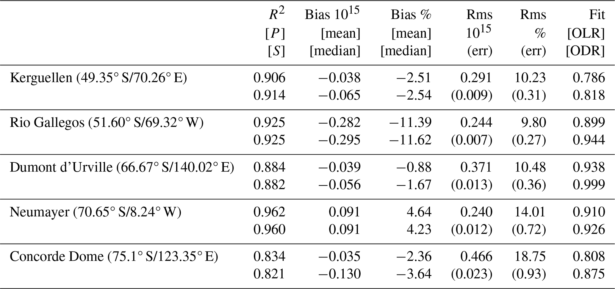
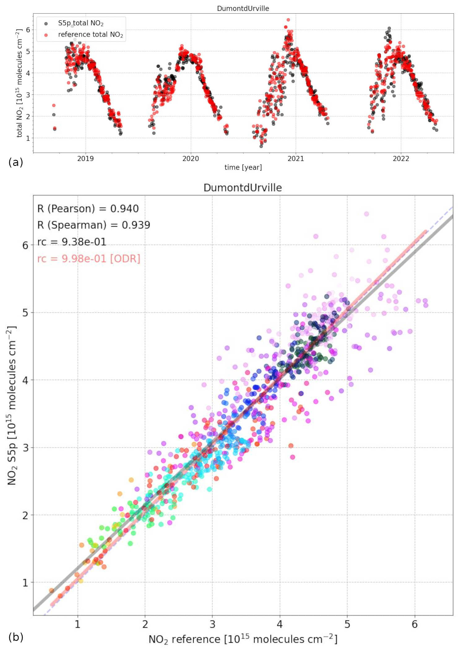
Figure 1 (a) Comparison of TROPOMI TNO₂ and SAOZ sunrise TNO₂ for the location of Dumont d'Urville. Data markers are semi-transparent to allow visually discriminating between overlapping SAOZ and TROPOMI data points. Note that for each SAOZ data point there is a corresponding TROPOMI data point. (b) Scatterplot of TROPOMI total NO₂ and SAOZ sunrise NO₂ as presented in Fig. 1a. Regression coefficients are for an ordinary linear regression (OLR; grey line) and the orthogonal distance regression (ODR; red line) with 1 : 1 line shown by the grey dashed line. Colors represent different times of the year (see Appendix Fig. A1 for the corresponding colored version of Fig. 1a).

Figure 1a shows a time series of the comparison of TROPOMI stratospheric NO₂ data with the SAOZ observations at the Antarctic site of Dumont d'Urville for the period 2018–2022. The Dumont d'Urville site is chosen as it is located sufficiently far north to provide good sampling of the seasonal stratospheric NO₂ cycle while also sampling both inner and outer Antarctic stratospheric-vortex air during local spring. Note that observations are missing during the middle of winter at Dumont d'Urville due to the polar night. Figure 1b shows the scatterplot of the same data.

Overall, the satellite measurements and ground-based measurements at Dumont d'Urville agree well (Table 1). The correlation coefficient is 0.88 (R²) with a bias of less than 2 % and root mean square differences of approximately 10 %. The regression coefficient equals 0.94 and almost 1.0 dependent on the regression method. The measurements at Dumont d'Urville during Antarctic springtime sample both inner- and outer-vortex air as evidenced by the rapid changes between large and small SNO₂ values during springtime. The validation results for Dumont d'Urville thus cover a wide range of atmospheric conditions. Results for the other four stations are rather similar (Table 1). Figures for the other four chosen validation sites can be found in the Appendix (Figs. A2 and A3) as well as on the TROPOMI validation server. The validation results for all stations can be summarized as follows.

• Correlations (R²) are always better than 0.80 and up to 0.96.

• Biases are of the order of a few percent (11 % for Rio Gallegos, Patagonia).

• Root mean square differences vary between 10 % and 20 %.

• Standard errors are smaller than 1 %.

• Regression values vary between 0.8 and 0.95.

• Results are fully consistent with Verhoelst et al. (2021).

• Results are fully consistent with Lambert et al. (2023).

Note that for Rio Gallegos the bias is larger than for the other four locations used here (ground-based total NO₂ columns larger than TROPOMI total NO₂ columns). One possible explanation could be that the SAOZ measurement location at Rio Gallegos is within 5 km from the edge of the buildup area of Rio Gallegos and 10 km from the city center. Lambert et al. (2023) found that for 42 polluted locations worldwide Pandora total NO₂ columns were on average approximately 18 % larger than corresponding TROPOMI total NO₂ columns, not unlike the 11 % bias for Rio Gallegos. For low pollution and clean locations the bias was smaller and reversed (TROPOMI total NO₂ columns approximately 6 % larger than Pandora total NO₂ columns). No large dependencies were found for the satellite solar zenith angle (SZA), the satellite cloud fraction, and satellite surface albedo. Given that Rio Gallegos is a city of approximately 80 000 inhabitants and its proximity to the SAOZ measurement site, it is not unlikely that Rio Gallegos SAOZ measurements could be contaminated by local air pollution under favorable wind conditions, although it is beyond the scope of this paper to investigate this in detail. Note that given the large seasonal cycle in total NO₂ columns an 11 % bias is still very acceptable.

Given that the typical seasonal cycle and differences between inner- and outer-vortex air vary by a factor of 2 to 5 and standard errors are a few percent or less combined with very high correlation coefficients and regression coefficients close to 1, single TROPOMI stratospheric NO₂ column measurements are of high quality and likely useful for in-depth exploration of spatiotemporal Antarctic stratospheric NO₂ variability.

2.3 Global ozone field data

In this study assimilated TROPOMI NO₂ column pixel data are used and gridded at a spatial resolution much coarser than the original TROPOMI resolution while also averaging in time due to multiple polar overpasses per day as the main interest in this first exploratory study is phenomena at continental scales. However, the TROPOMI NO₂ column pixel data are also already post-processed level-2 observations, i.e., TROPOMI NO₂ data derived from a data assimilation system and in that sense not pure level-2 pixel data anymore. Hence, it was decided to compare the TROPOMI NO₂ data with gridded assimilated TCO₃ data rather than TCO₃ data at orbit level. An obvious TCO₃ dataset to use would be the Multi-Sensor Reanalysis version 2 (MSR-2; van der A et al., 2010, 2015a), which provides a global reanalysis of TCO₃ combining multiple and sometimes overlapping satellite measurements using an advanced ground-data-based approach to minimize inter-satellite-instrument TCO₃ differences and biases. However, the MSR-2 TCO₃ dataset had not yet been extended in time to cover the entire period for which TROPOMI NO₂ data were available. Hence the KNMI operational daily global assimilated TCO₃ field is used here (Eskes et al., 2003; van der A et al., 2015a; https://www.temis.nl/protocols/O3global.php, last access: 6 December 2022), which is based on TCO₃ level-2 data products of the GOME-2 instruments aboard the MetOp satellites (Munro et al., 2006, 2016). This operational TCO₃ field is produced by KNMI for operational UV index predictions up to 9 d ahead in time. GOME-2-based TCO₃ analyses are thus always available in real time – unlike MSR-2, which is currently updated only once per year. From this operational TCO₃ dataset the global total ozone field at each longitude at local solar noon is used, which is close to the TROPOMI measurement time (Sect. 2.1) and which is available for every day of the year for the full globe. The local solar noon ozone field is, for example, used for the operational Tropospheric Emission Monitoring Internet Service (TEMIS) UV index and UV dose processing (van Geffen et al., 2017; Zempila et al., 2017). The local solar noon global TCO₃ field is given at a longitude–latitude grid of 1.5° × 1.0° and is re-gridded (bilinear interpolation) to a finer 0.8° × 0.4° to match the gridded NO₂ data. Note that differences between the KNMI operational daily global assimilated TCO₃ data and the MSR-2 TCO₃ data are small. GOME-2 has a 4 DU offset relative to ground observations (MSR-2 has none), but otherwise GOME-2 and MSR-2 have similar root mean square differences compared to ground observations (van der A et al., 2015a). Hence, for the purpose of this study both datasets would be interchangeable. The question of using assimilated TCO₃ data rather than collocated TROPOMI TCO₃ orbit data will be discussed in Sect. 4.

3 Data analysis and results

3.1 Spatiotemporal variability

Figure 2 shows maps of the spatial distribution of SNO₂ and TCO₃ at local solar noon on 1 November 2018 as an example of daily data. In both panels a black line displays the TCO₃ = 200 DU contour, a not uncommon reference value to mark the edge of the Antarctic ozone hole for the Southern Hemisphere polar vortex.

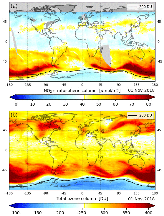
Figure 2 Maps of globally gridded TROPOMI-based stratospheric NO₂ (a) (in µmol m⁻²) and globally gridded local solar noon assimilated TCO₃ (b) (in Dobson Units or DU) on 1 November 2018. The location of the 200 DU ozone contour is indicated by a black line in both panels. Grey denotes areas without TROPOMI data.

SNO₂-depleted Antarctic inner-vortex air and enhancement of SNO₂ around the edge of the polar vortex are clearly visible. Figure 3 shows the same data as in Fig. 2 but for an Antarctic polar view and with a different color scale. There are clear similarities between the spatial patterns in SNO₂ and TCO₃. First of all, both show a significant reduction of values within the Antarctic stratospheric vortex. Secondly, values for both are strongly enhanced equatorward just outside of the vortex. Third, further equatorward of 45° S values of both start to decrease. And fourth, outside of the vortex values for both are reduced around 0° longitude and enhanced at the opposite side towards 180° longitude (wave-1 pattern).

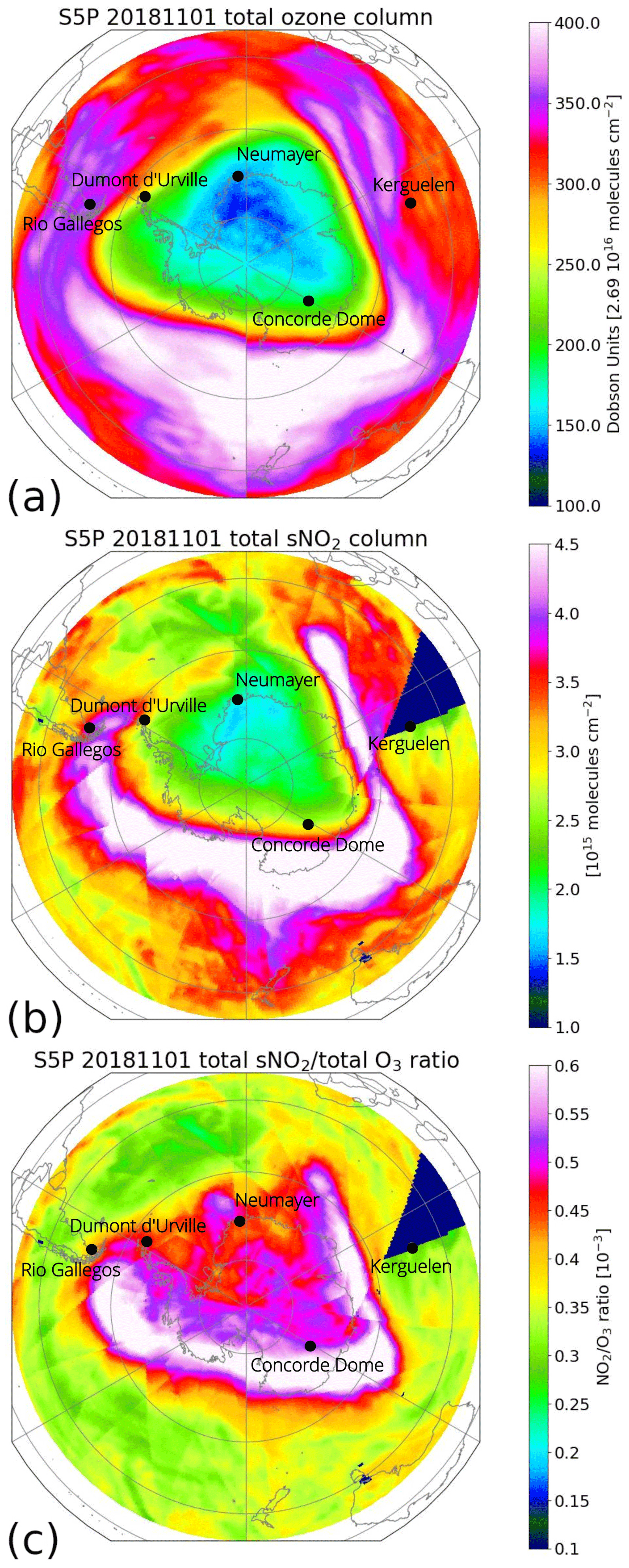
Figure 3 As Fig. 2 (1 November 2018) but from an Antarctic polar view and with a different color scale. Panel (c) shows the SNO₂ $/$ TCO₃ ratio of panels (a) and (b).

However, there are also clear differences. The SNO₂ $/$ TCO₃ ratio, for example, does not show a clear vortex edge (Noxon cliff) like in both separate products. Furthermore, the gradient from the vortex edge towards the Equator is smaller for TCO₃ than it is for SNO₂. These similarities and differences point to different processes governing their respective spatiotemporal variations: chemistry (sources and sinks) and stratospheric dynamics (source and sink regions and transport from sources to sinks).

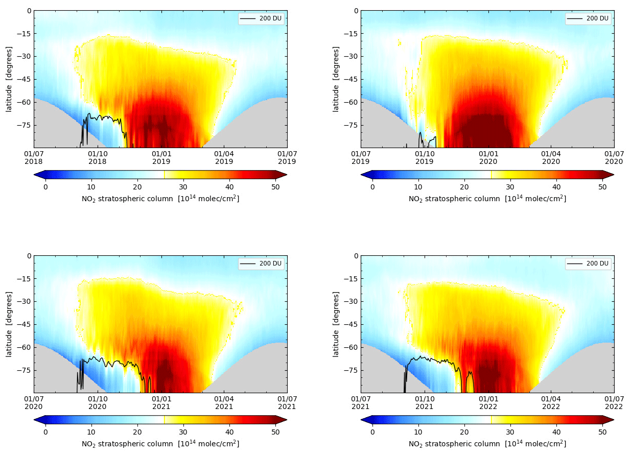
Figure 4 Maps of the Southern Hemisphere daily zonal average SNO₂ for four Southern Hemisphere summers (July–July) from 2018 to 2022. The location of the 200 DU ozone contour is indicated by a black line in all panels. Grey denotes areas and times within TROPOMI data.

Figure 4 shows the evolution of zonal averages of SNO₂ during the four Southern Hemisphere summers from 2018 to 2021, with the 200 DU ozone contour indicated by a black line. From these figures it is clear that springtime advection of SNO₂-enhanced stratospheric air into the Antarctic stratospheric vortex is limited during 2018, 2020, and 2021. The lack of such a well-defined SNO₂-depleted area in 2019 is related to the weak Antarctic stratospheric vortex during spring 2019, which led to weak ozone depletion (Safiedinne et al., 2020; Wargan et al., 2020; Stone et al., 2021) and according to the TROPOMI NO₂ data thus also led to less denitrification. This is consistent with results from IASI HNO₃ (Wespes et al., 2022).

3.2 Correlating SNO₂ and TCO₃: 2D phase diagram

Figure 5 displays TROPOMI TCO₃ and SNO₂ data for 1 November 2018 as a 2D histogram (phase diagram; Fig. 5a) revealing rather intricate patterns. For reasons explained below, the histogram was divided into three areas to be able to discriminate between the inner vortex (MASK-1), outer vortex (MASK-2), and vortex edge (MASK-3). For the area MASK-1 SNO₂ and TCO₃ show a well-defined linear relationship. The area is associated with the inner vortex and is characterized by small TCO₃ values. The area MASK-2 represents air outside of the vortex characterized by larger TCO₃ values and somewhat larger SNO₂ values than for the MASK-1 area. Also, there is not such a well-defined linear relation between TCO₃ and SNO₂ for the MASK-2 area as there is for the MASK-1 area. The relation between TCO₃ and SNO₂ for MASK-3 is much more intricate with what appear to be “coherent line structures” connecting the MASK-1 and MASK-2 areas. These “mixing lines” – for lack of a better expression – are found for both small and large TCO₃ and SNO₂ values. The largest SNO₂ values are found in the MASK-1 and MASK-3 areas, whereas the largest TCO₃ values are found in the MASK-2 and MASK-3 areas. Note that the logarithmic color scale enhances the focus on parts of the distribution that are less frequent. There are thus essentially two populations: inside the vortex and outside the vortex. A total of 16 % of the histogram bins contain two-thirds (∼ 67 %) of the data points and only approximately 10 % of the data qualify for MASK-3.

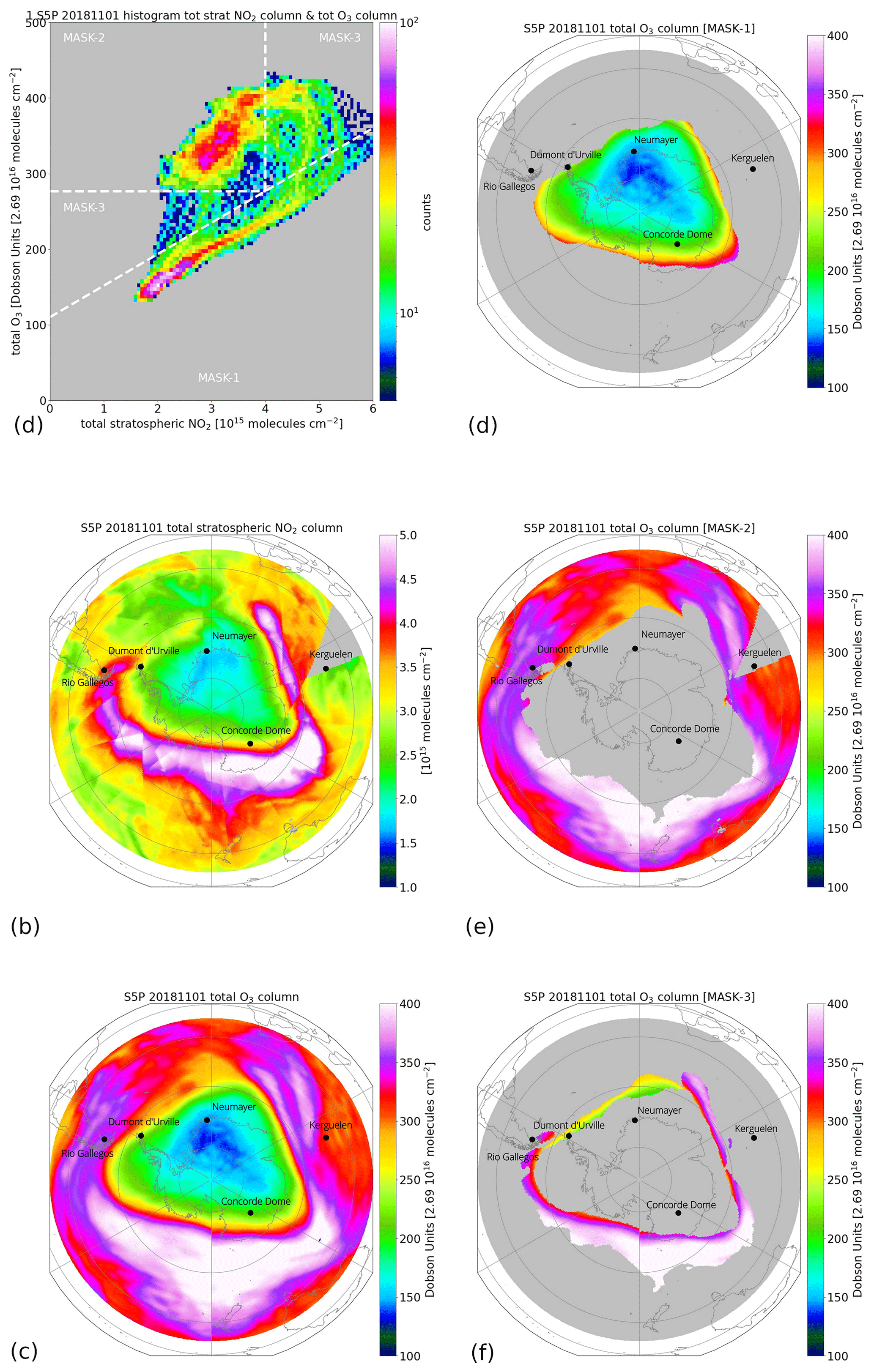
Figure 5 (a) 2D histogram (phase diagram) of TROPOMI SNO₂ vs. assimilated TCO₃ for 1 November 2018 and corresponding spatial distribution of SNO₂ (b) and TCO₃ (c) as in Fig. 3. The phase diagram is color-coded according to the logarithm of the number of counts. The phase diagram is a 100 × 100 pixel grid ranging between 0.0–6.0 × 10¹⁵ molec. cm⁻² SNO₂ and 0–500 DU TCO₃. (d–f) Spatial distribution of TCO₃ as in the lowest plot of the left column but filtered on the masking in the phase diagram in the upper left plot. (d) MASK-1, (e) MASK-2, (f) MASK-3.

3.3 Multi-day periods and multi-annual data

A key follow-up question is whether these results change significantly over time. Figure 6 shows phase diagrams similar to the one displayed in Fig. 5 but for days combined during multiple-day intervals (5, 10, 15, and 30 d) starting at 1 November 2018. Although this means that each panel covers a different time period, the results are nevertheless very consistent. The distinction of two clear concentrated populations and the mixing lines is present for each time period. The results also reveal a relation between TCO₃ and SNO₂ outside of the vortex, albeit with a much larger spread. The high correlation between TCO₃ and SNO₂ inside the vortex is also present during all periods. The distribution does shift towards larger SNO₂ values due to increasing SNO₂ as part of the natural springtime SNO₂ cycle. Similarly, although more difficult to distinguish in Fig. 6, outer-vortex TCO₃ values become slightly smaller due to the natural seasonal springtime non-catalytic photochemical destruction of stratospheric O₃. However, for inner-vortex air the TCO₃ distribution shifts towards larger TCO₃ values, reflecting the effects of dynamical mixing of extra-vortex O₃-rich (upper-)stratospheric air during late spring (de Laat and van Weele, 2011).

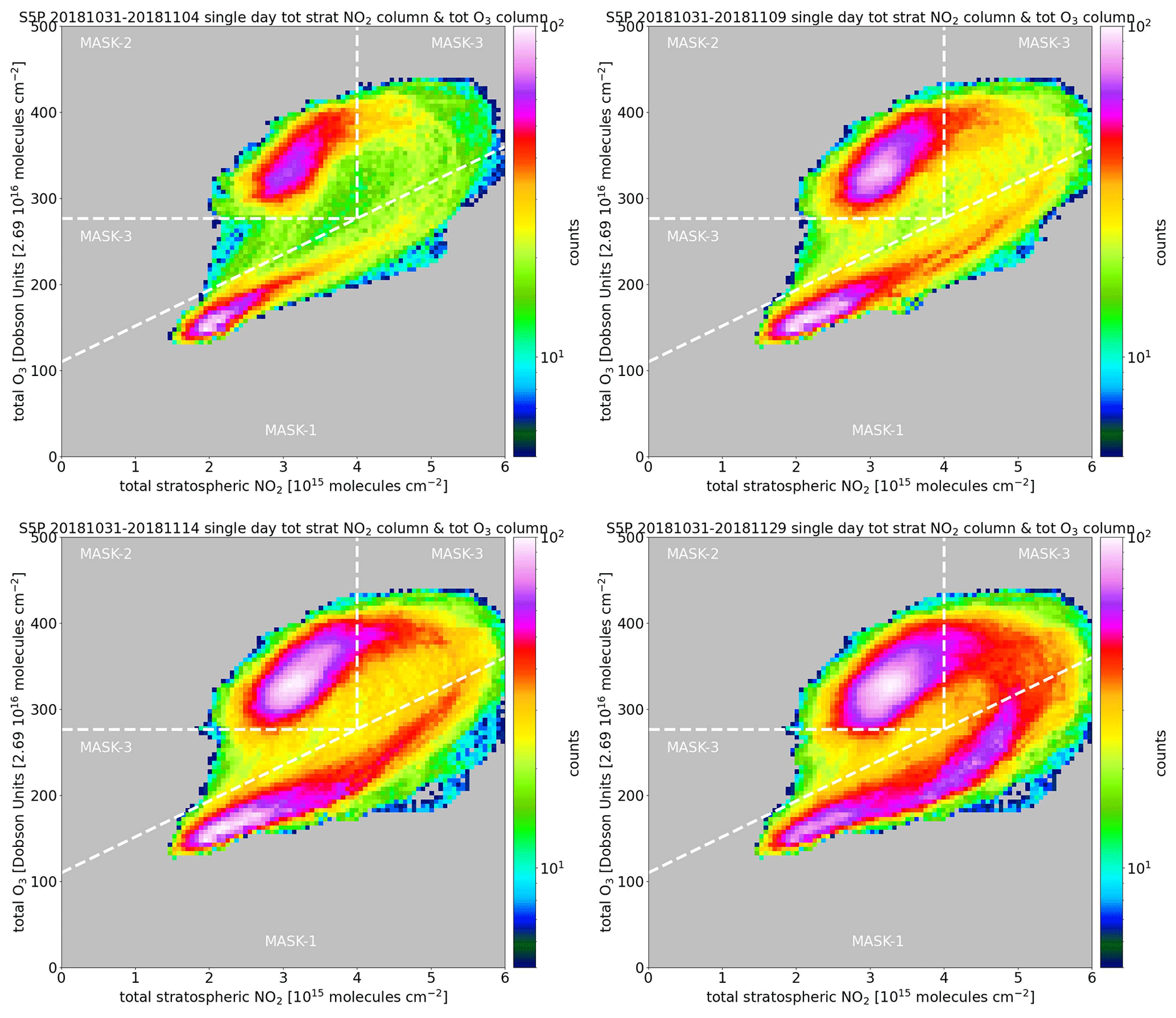
Figure 6 Phase diagrams of TROPOMI SNO₂ and assimilated GOME-2 TCO₃. Similar to the phase diagram in Fig. 5a but for daily gridded data combining either 5, 10, 15, or 30 d starting at 31 October 2018.

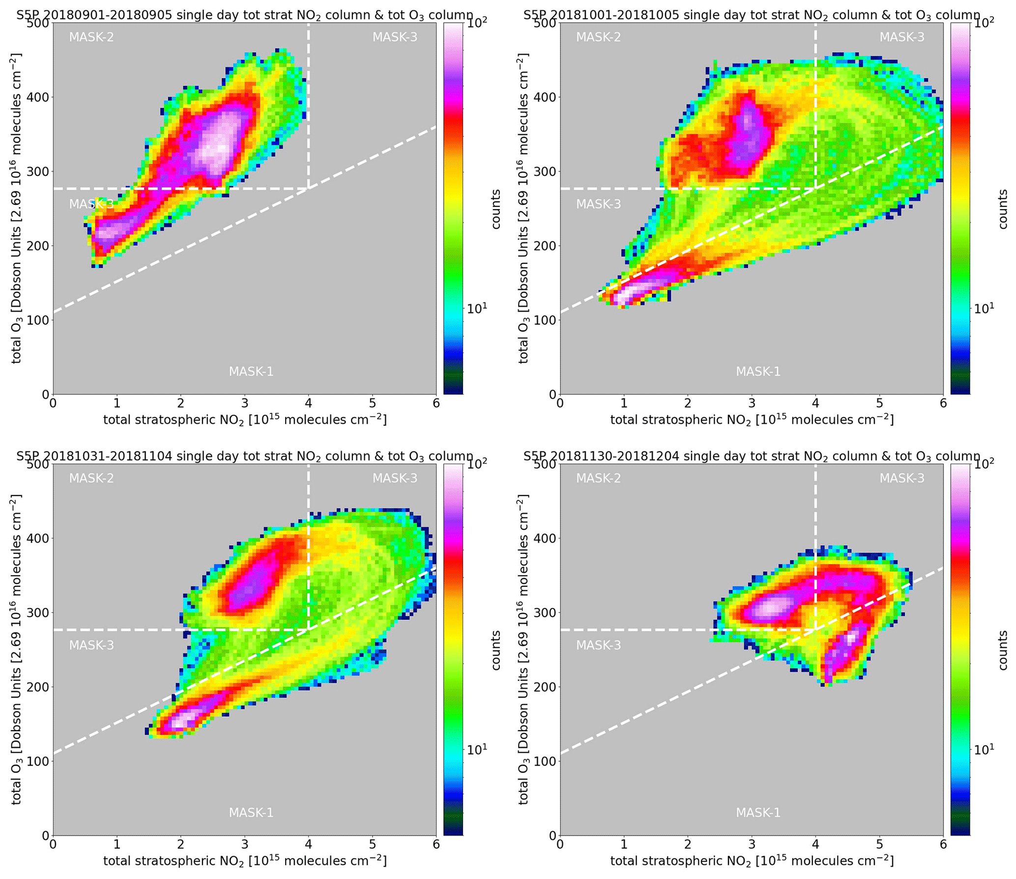
Figure 7 As Fig. 6 but for 5 d periods starting at 1 September, 1 October, 31 October, and 30 November 2018.

Figure 7 shows similar panels as in Figs. 5 and 6 but for 5 d periods starting at the first day of each month from September to December 2018. The results are much more variable than for the multi-day differences, highlighting the strong seasonality of Antarctic stratospheric inner-vortex TCO₃ and SNO₂. During early September O₃ depletion has yet to commence. There are already two separate populations discernible but TCO₃ values are still larger than 200 DU. SNO₂ values are generally small, especially within the Antarctic vortex due to the denitrification process. In early October 2018 the catalytic O₃ destruction has strongly reduced stratospheric O₃. There is a group of data points with small TCO₃ values and small SNO₂ values. The air outside of the vortex is still characterized by large TCO₃ values and still relatively small SNO₂ values but larger values than during early September 2018. The mixing lines are also clearly discernible, covering the entire phase space between the two main populations. The picture for early November 2018 is rather similar, although SNO₂ values have further increased due to the natural seasonal cycle in SNO₂. By early December 2018 the distribution is squeezed and values from both main populations are closer together. The vortex has largely disintegrated, although remnants can still be discerned in TCO₃ but interestingly enough not in SNO₂ (see animation in the Supplement). Remarkably the populations still cover the three previously defined areas MASK-1, MASK-2, and MASK-3. This indicates that TCO₃ $/$ SNO₂ ratios are rather useful for characterizing the origins and locations of stratospheric air masses.

Figure 8 As Fig. 6 but for 1–30 October of each year between 2018 and 2021.

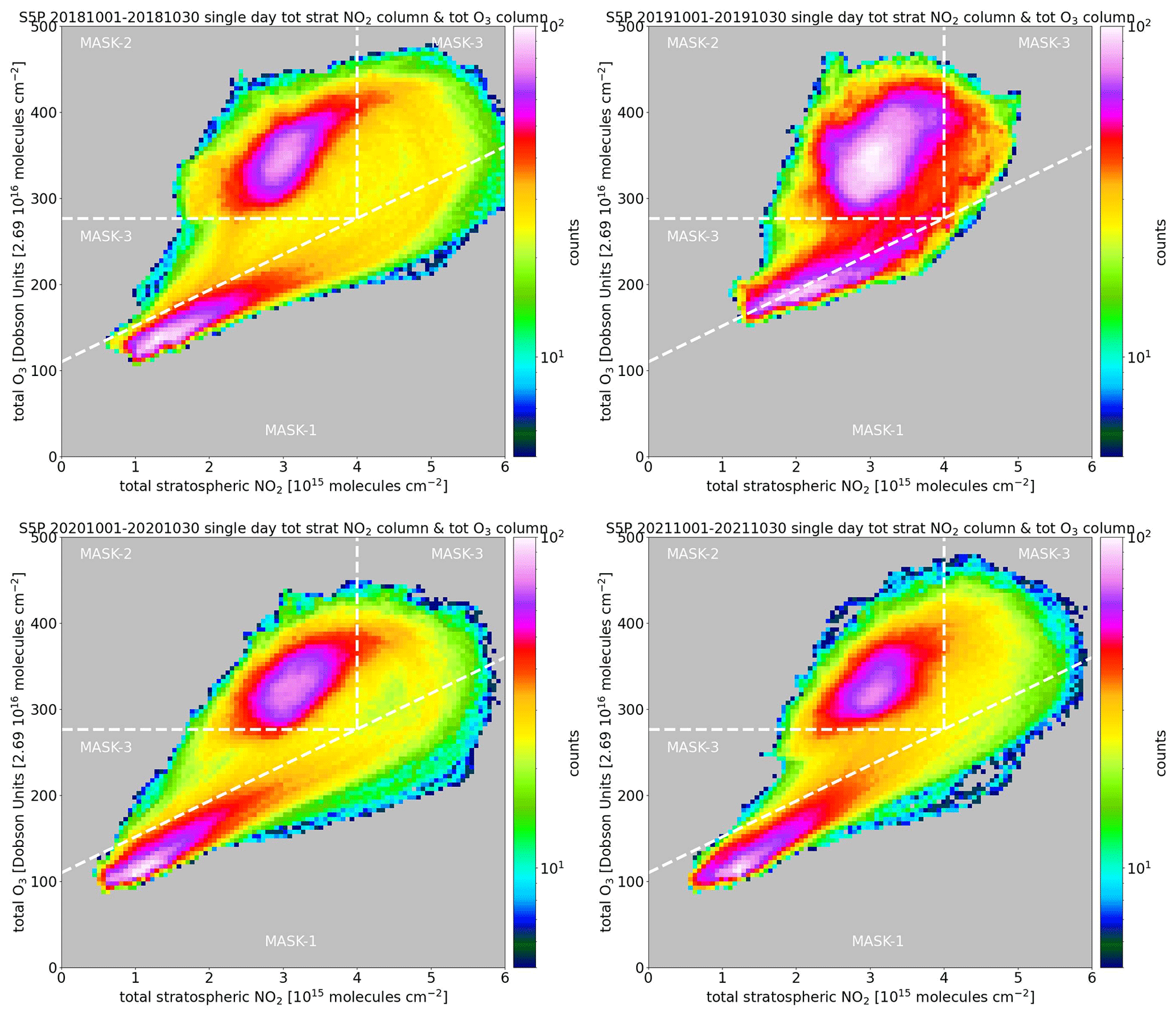
Figure 8 displays similar results as in Fig. 7 for early October but for all years from 2018 to 2021. The results for 2018, 2020, and 2021 are very similar, providing further support for the notion that the TCO₃ $/$ SNO₂ ratios can be used to characterize the origins and locations of stratospheric air masses. The results for 2019 are quite different, reflecting the unusually weak 2019 Antarctic stratospheric vortex. There are still two populations in 2019 but only weakly separated. TCO₃ and SNO₂ values inside the vortex are larger compared to the other years. Overall, the anomalous 2019 vortex has a clear imprint on the TCO₃ and SNO₂ distributions. Note that during early September 2019 the amount of SNO₂ depletion was still similar to those in 2018, 2020, and 2021 (not shown). The normal vortex pre-conditioning during austral winter 2019 was thus not unusual, which is consistent with published analyses of the 2019 Antarctic springtime vortex (Wargan et al., 2020; Smale et al., 2021; WMO, 2022). The faster 2019 increase in SNO₂ by early October compared to 2018, 2020, and 2021 indicates that dynamics and mixing with – or influx of – NO₂-rich extra-vortex air are the main cause. Otherwise the SNO₂ increase would have been slower and more in line with the other 3 years.

3.4 Qualitative explanation of phase diagram results

The consistency of patterns in the spatiotemporal variations in the TCO₃–SNO₂ distributions suggests some very basic underlying processes. For example, differences in the location of the TCO₃ cross-vortex gradient relative to the location of the Noxon cliff for SNO₂ should show up as patterns in the phase diagram. To provide a qualitative explanation of the observed patterns two simple series of longitudinal and latitudinal variations in TCO₃ and SNO₂ were created. For the first one, TCO₃ and SNO₂ vary as a sine wave along longitudes but with a different longitudinal phase (Fig. 9). For the second one, TCO₃ and SNO₂ increased from the poles to middle latitudes and then decreased toward the Equator to resemble the Noxon cliff but with a slightly different latitudinal change visually mimicking the observed TCO₃ and SNO₂ latitudinal gradients. Figure 9 shows the results for the relation between the two. For the phase-shifted sine wave functions, the results obviously show up as an oval. The latitudinal shifted results, however, follow a curve not qualitatively dissimilar from the observed mixing lines. These results thus support the observation that the cross-vortex TCO₃ gradient and SNO₂ Noxon cliffs do not occur at the same locations, which results in the emergence of mixing lines in the phase diagrams.

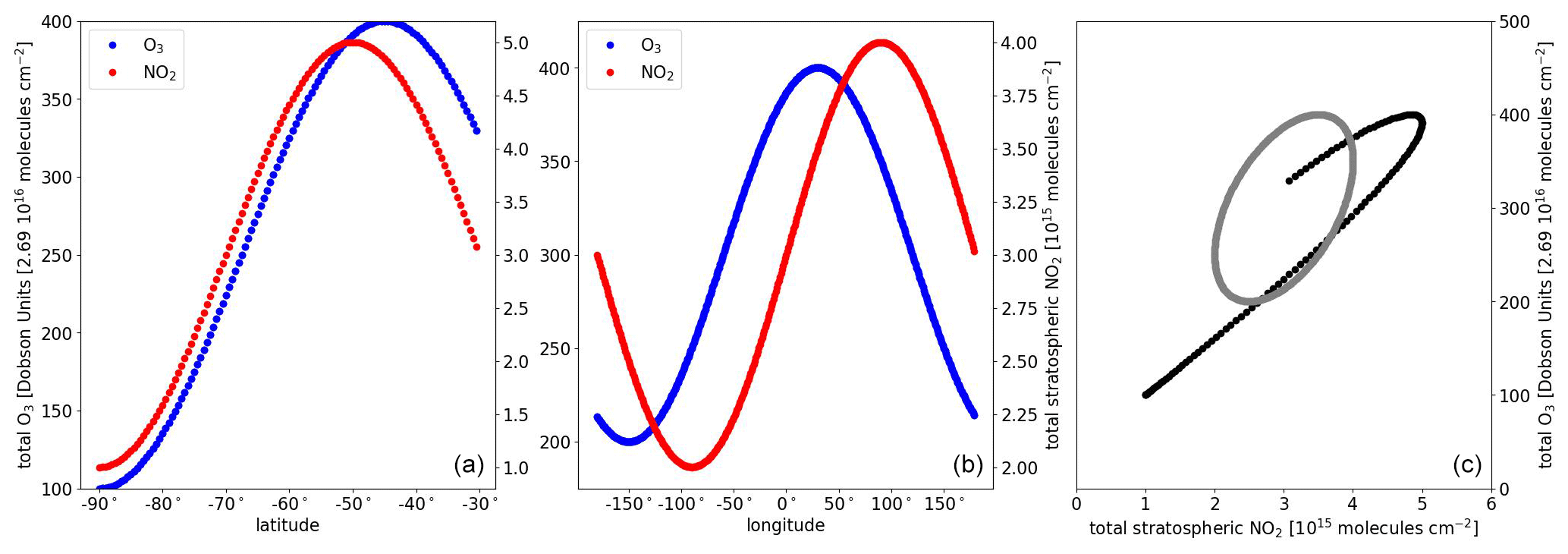
Figure 9 (a) Latitudinal SNO₂ and TCO₃ variations between 30 and 90° S. The functions for SNO₂ and TCO₃ are slightly shifted in the latitudinal direction, with SNO₂ peaking earlier and decreasing faster towards the Equator after the peak. The result of these two functions is indicated by the black line in panel (c). (c) Longitudinal data and phase diagram of a data series (sine wave) for SNO₂ (red) and TCO₃ (blue) with a longitudinal phase shift of 90°. The amplitude of the sine wave is chosen to represent observed values but otherwise just a scaling factor. The result for these two functions is indicated by the grey line in panel (c).

4 Discussion

The results presented here show that TROPOMI provides high-quality daily SNO₂ data for monitoring variations in SNO₂ both inside and outside the Antarctic stratospheric vortex. It allows for studying the nitrogen hole, the denitrification process, and the Noxon cliff – the sharp gradient in trace gas amounts along the vortex edge – as well as associated seasonal changes during Antarctic springtime and interannual variability. Furthermore, combining the SNO₂ data with high-quality TCO₃ data in phase diagrams reveals coherent patterns – mixing lines – linking the Antarctic stratospheric air inside and outside the vortex.

A clear discrepancy was found between the location of the SNO₂ Noxon cliff and the TCO₃ cross-vortex gradient. The few studies that provide information on the joint vertical distributions of NO₂ and O₃ suggest that the bulk of stratospheric NO₂ is found at higher altitudes than the bulk of stratospheric O₃ (Ridley et al., 1984; Lindenmaier et al., 2011). Differences in bulk heights, which mostly determine total column variability, link to differences in advection processes and might explain differences in the location of the NO₂ Noxon cliff and the cross-vortex TCO₃ gradient. Explorative studies using stratospheric chemistry models should likely help unravel these issues. This in turn may contribute to developing applications and metrics for stratospheric NO₂-column-based Antarctic ozone hole monitoring. In addition, the notion of different bulk heights is consistent with the notion that the break-up dates or final warming of the Antarctic stratospheric vortex occurs later for lower-stratospheric altitudes (higher pressure levels) (Butler and Domeisen, 2021; Lecouffe et al., 2022). For example, by late November 2018 there is still a well-defined area with reduced TCO₃ for which reduced SNO₂ has already vanished (see animation in the Supplement). A lower bulk height for TCO₃ compared to SNO₂ would mean that SNO₂ anomalies would vanish earlier, as observed.

Furthermore, a strong inner-vortex correlation between SNO₂ and TCO₃ was found, which was absent outside of the vortex. The SNO₂–TCO₃ phase diagrams display a clear dynamical cycle reflecting springtime changes in chemistry and dynamics. This cycle was consistently seen in multiple years (2018, 2020, and 2021) but was significantly different in 2019, a year with a strongly perturbed Antarctic springtime vortex. Qualitatively the coherent patterns in the phase diagrams can be explained by spatiotemporal differences in the phases of SNO₂ and TCO₃, i.e., where and when minima and maxima occur in SNO₂ and TCO₃. SNO₂ and TCO₃ are clearly not always in sync everywhere. This in part appears to be associated with the differences in Antarctic stratospheric denitrification and O₃ depletion. Denitrification is a wintertime process already starting by early winter and causing the Antarctic stratosphere to be significantly depleted of nitrogen by the time sunlight returns (and thus TROPOMI starts to provide inner-vortex observations). The O₃ destruction cycle, on the other hand, critically depends on the presence of sunlight. At the start of springtime O₃ depletion has yet to speed up. During the month of September the amount of sunshine and duration of sunshine rapidly increase, causing a rapid deepening of the Antarctic ozone hole. Hence, the denitrification and O₃ depletion cycles differ significantly in their timing. Similarly, the results also revealed an earlier disappearance of the NO₂ hole relative to the ozone hole, further supporting the notion that differences in chemistry and dynamics govern the differences in SNO₂ and TCO₃ behavior.

The observation of coherent spatial line structures (mixing lines) in relation to stratospheric transport and mixing – including stratosphere–troposphere exchange – is not new. The presence of layered trace gas structures in the stratosphere (laminae, filamentation, contour advection; Waugh and Plumb, 1994; Newman et al., 1996; Appenzeller and Holton, 1997; Orsolini and Grant, 2000; Koh and Legras, 2002) is closely associated with the stability of the stratosphere, the conservation of potential vorticity, and isentropic mixing (Waugh and Polvani, 2010). Stratospheric air masses often organize themselves in such long-lived laminae. For example, satellite observations of direct injection of volcanic material directly into the (lower) stratosphere have provided many examples of laminae development and filamentation because of the ability of satellites to observe sulfur dioxide and volcanic ash (Krotkov et al., 2021; de Leeuw et al., 2021; Khaykin et al., 2022). Satellite observations of aerosols from wildfires have started to be used for similar purposes for stratospheric smoke (Khaykin et al., 2020; Magaritz-Ronen and Raveh-Rubin, 2021). And complex relationships among (long-lived) stratospheric trace gases have been used for understanding stratospheric dynamics (e.g., Hoor et al., 2002; Plumb, 2007; Barré et al., 2012; Hoffmann et al., 2017; Krasauskas et al., 2021). How exactly these processes and concepts relate to the observed mixing lines would make a relevant topic of future research.

Furthermore, model simulations could be used to assess (1) whether model simulations show similar phase diagrams and, if so, (2) whether the model simulations contain clues for explaining the differences in spatiotemporal SNO₂ and TCO₃ behavior. The model simulations might also reveal caveats and missing processes in the model representation of stratospheric chemistry and Antarctic stratospheric vortex dynamics. In addition, the results can also be further explored towards a more thorough conceptual explanation of SNO₂ variability. Comparison with IASI HNO₃ total columns might help there as well, just like a comparison and evaluation of SNO₂ with satellite NO₂ profile measurements from, for example, the OSIRIS (Optical, Spectroscopic and Infrared Remote Imaging System), ACE-FTS (Atmospheric Chemistry Experiment – Fourier Transform Spectrometer), or MAESTRO (Measurements of Aerosol Extinction in the Stratosphere and Troposphere Retrieved by Occultation) satellite instruments. A comparison with IASI HNO₃ could, for example, be used to explore whether both are more in sync than SNO₂ is with TCO₃. Comparison with limb satellite NO₂ profile measurements in conjunction with O₃ profile measurements should provide indications of which altitudes mostly determine column observations of NO₂ and O₃. In addition, evaluation of results from a different dynamical framework of the equivalent latitude might help improve understanding of Antarctic stratospheric vortex-edge dynamics. This links to the important question of where and when vortex mixing takes place. It is well established that the Antarctic stratospheric vortex can be destabilized by increased extra-vortex wave activity. Direct observations of where and when that takes place are unclear but the combination of SNO₂ and TCO₃ (possibly extended with IASI HNO₃) might help identify mixing regions.

An additional question is whether satellites other than TROPOMI that also measure SNO₂ might help extend the SNO₂ Southern Hemisphere record further back in time. A dataset going back to 2003 already exists via the QA4ACV NO₂ data (Quality Assurance for Essential Climate Variables; Boersma et al., 2018). The combination of GOME (1995–2011), SCIAMACHY (2002–2012), OMI (2003–now), GOME-2 (2007–now), and OMPS (2012–now; Ozone Mapping and Profiler Suite) potentially allows for reconstructing an almost 30-year record of Southern Hemisphere midlatitude and Antarctic SNO₂. Such a record could be probed for finding hints and clues of (Antarctic) stratospheric ozone recovery, as TCO₃ is expected to change much faster due to decreasing O₃-depleting substances than SNO₂ – mostly due to emissions of N₂O and slowly increasing atmospheric N₂O concentrations (Struthers et al., 2004). Other processes relevant for Antarctic stratospheric NO₂ and O₃ are production of (upper-)stratospheric NO_x by energetic electron precipitation and by increased downwelling of upper-stratospheric air by the expected speeding up of the Brewer–Dobson circulation (Gordon et al., 2020; Maliniemi et al., 2021; Müller, 2021).

Furthermore, there are some other aspects for further exploration. The validation could be extended to more ground-based comparison and more detailed evaluations. It could be assessed whether it matters if TNO₂ is used (based on data assimilation) rather than SNO₂. The assimilation SNO₂ data are important for deriving tropospheric NO₂ but not necessarily the best estimate of TNO₂. Note that there is no reason to assume that SNO₂ and/or TCO₃ data quality issues will change the findings of this paper, but only in-depth analyses will provide support for that assumption. In addition, although the diurnal cycle in SNO₂ is relatively small compared to its seasonal cycle it nevertheless can affect satellite retrievals and validation results. Dubé et al. (2021) reported order-of-magnitude 10 %–20 % diurnal cycle effects for SAGE III/ISS solar occultation limb retrievals with the largest effects found at higher latitudes. Although their results are not one-on-one applicable to the results presented here they clearly indicate the need for properly assessing diurnal cycle effects on TROPOMI SNO₂ measurements and validation.

In this study gridded SNO₂ was used to allow easy comparison with other data as TROPOMI data quality is still improving and reprocessing of data is ongoing. A key question is whether results would differ for a TROPOMI pixel-level comparison of SNO₂ and TCO₃. A first brief assessment of using TROPOMI pixel-level comparison of SNO₂ and TCO₃ (see Appendix Fig. A4) yielded very similar results, indicating that results presented here are robust relative to using gridded data, pixel data, or even data from different satellites.

Finally, limited use of nadir-viewing satellite measurements of NO₂ for studying the Noxon cliff and the Antarctic stratospheric denitrification process is somewhat surprising. The potential for their use to explore polar stratospheric chemistry and dynamics is evident from Wenig et al. (2004), Richter et al. (2005), and Adams et al. (2013). Satellite measurements of NO₂ – and tropospheric NO₂ column measurements – have been widely used for approximately 2 decades now. Total stratospheric NO₂ columns play an important role in deriving tropospheric NO₂ columns, as the stratospheric part needs to be removed from the total part (Boersma et al., 2004, 2007, 2018). This is typically done by assimilating the satellite measurements of total NO₂ over clean regions into a numerical chemistry transport model to reconstruct the stratospheric column globally (Eskes et al., 2003; Boersma et al., 2004, 2007). The assimilation therefore allows determining the stratospheric column over polluted regions with sufficient accuracy and precision to subtract it from the total column to arrive at an accurate tropospheric column. This approach also requires sufficiently accurate measurements of stratospheric NO₂. Hence the quality of stratospheric NO₂ has for a long time been assessed for various satellites (e.g., Boersma et al., 2004; Dirksen et al., 2011; Valks et al., 2011; Verhoelst et al., 2021; Lambert et al., 2023). Nevertheless, despite the fact that nadir stratospheric NO₂ column TROPOMI measurements turn out to be of very good quality their intrinsic value for stratospheric research has remained largely unrecognized.

5 Conclusions

This paper presents a first assessment of the use of Sentinel-5p TROPOMI SNO₂ measurements for studying Southern Hemisphere middle-latitude and Antarctic stratospheric processes including the Antarctic ozone hole.

Comparison of gridded SNO₂ and assimilated TCO₃ via phase diagrams reveals intricate patterns. Three different regimes could be clearly identified: the inner vortex, the vortex edge, and the extra-vortex region. Each regime is associated with its own SNO₂ $/$ TCO₃ characteristics. The vortex edge was characterized by so-called “mixing lines” in SNO₂–TCO₃ phase diagrams. A certain misalignment of the SNO₂ Noxon cliff and cross-vortex TCO₃ gradient was found along the Antarctic stratospheric vortex, pointing to vortex-edge dynamics as the root case. A possible explanation could be differences in bulk heights of SNO₂ and TCO₃ so that their respective total columns reflect processes occurring at different heights.

Springtime SNO₂–TCO₃ variations and changes are robust throughout single-day to multi-day statistics. Throughout spring the SNO₂–TCO₃ distributions change significantly as a result of chemistry and vortex dynamics including mixing of air inside and outside the vortex. Regarding interannual variability the distributions are very similar for 2018, 2020, and 2021 but significantly different from 2019, which was a year with an anomalously weak Antarctic stratospheric vortex and only weak O₃ depletion.

Seasonal changes in the phase diagrams indicate that both total column data products are sensitive to different heights and thus different processes. In general the vortex remains visible longer in TCO₃ data than in SNO₂ data. SNO₂ is less sensitive to the lower stratosphere – where the stratospheric vortex remains intact longer – than SNO₂ so the nitrogen hole will disappear earlier than the ozone hole. Vertical tilting of the vortex edge combined with different vertical sensitivities likewise explains the presence of the third regime: that in the phase diagrams linking the inner-vortex regime with the outer-vortex regime.

This study only presents a first glimpse of the great potential of high-quality spatiotemporal satellite SNO₂ measurements for studying stratospheric chemistry and stratospheric dynamics as well as long-term changes in stratospheric composition extending the SNO₂ record back in time in combination with, for example, the MSR-2 total ozone reanalysis (van der A et al., 2015a). The ability to monitor stratospheric nitrogen is also more than welcome given that an important piece of stratospheric observational remote sensing capacity by way of the Microwave Limb Sounder (MLS) will end by 2025 or at the latest 2026 and no satellite missions are planned to fill the gap created by the end of the MLS mission.

Appendix A

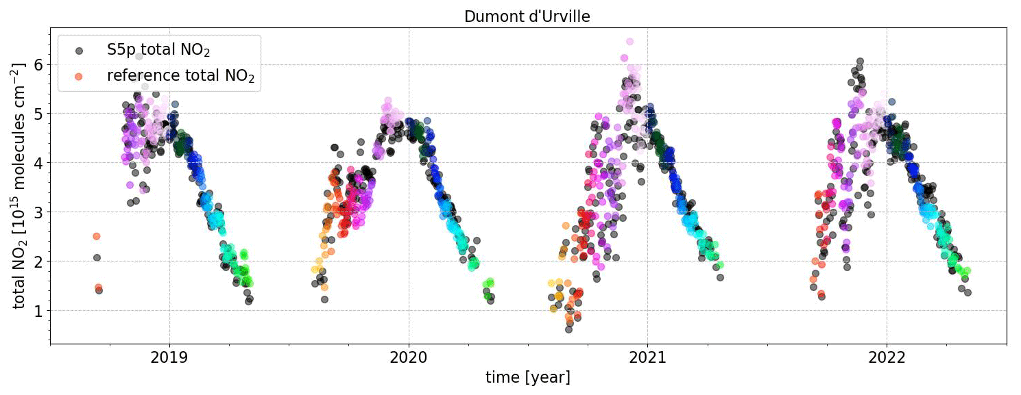
Figure A1 As Fig. 1a but color-coded according to time of the year (color coding also used in Fig. 1b).

Figure A2 As Fig. 1a but for the other surface measurement stations in Table 1.

Figure A3 As Fig. 1b but for the other surface measurement stations in Table 1.

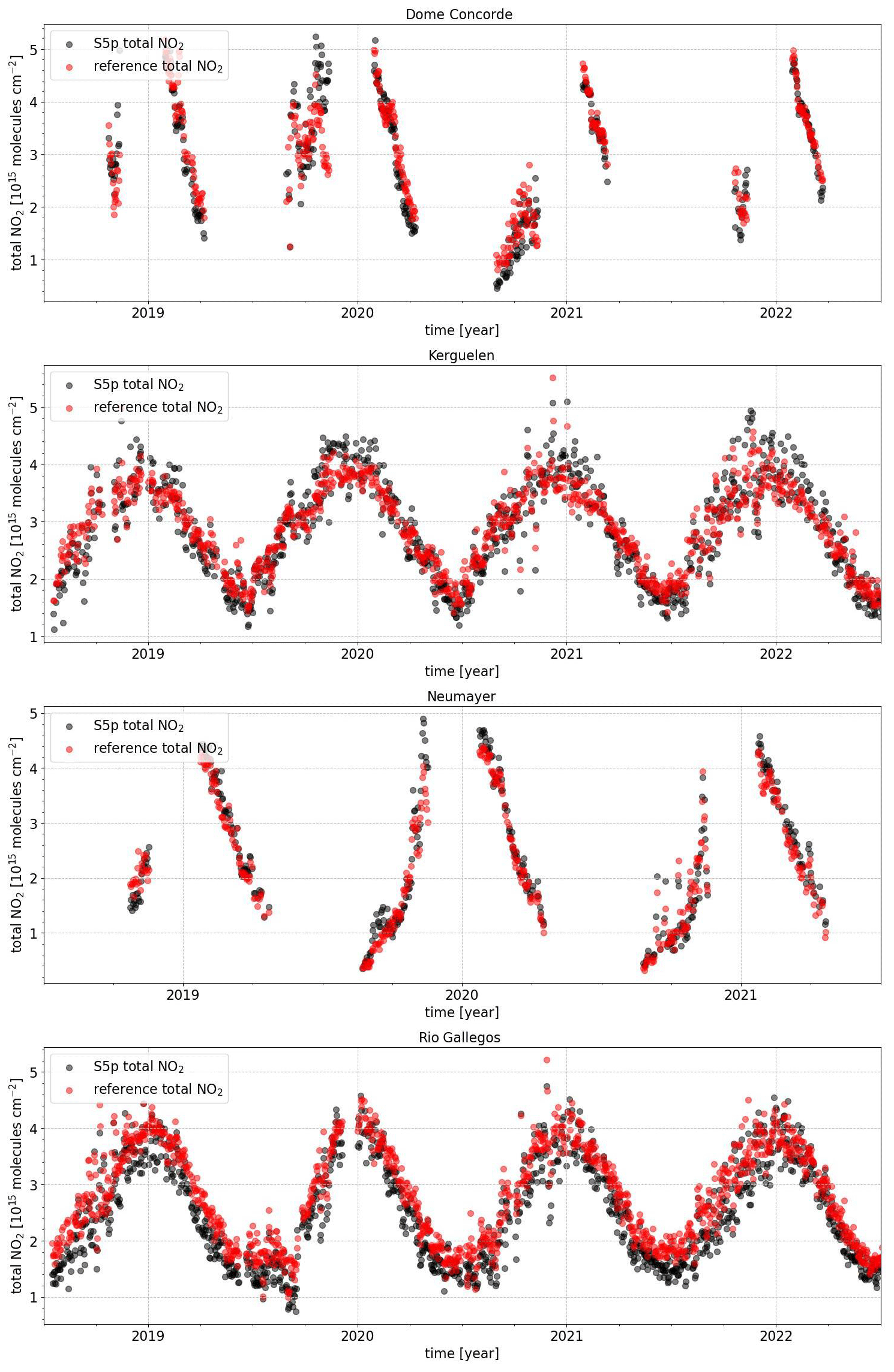
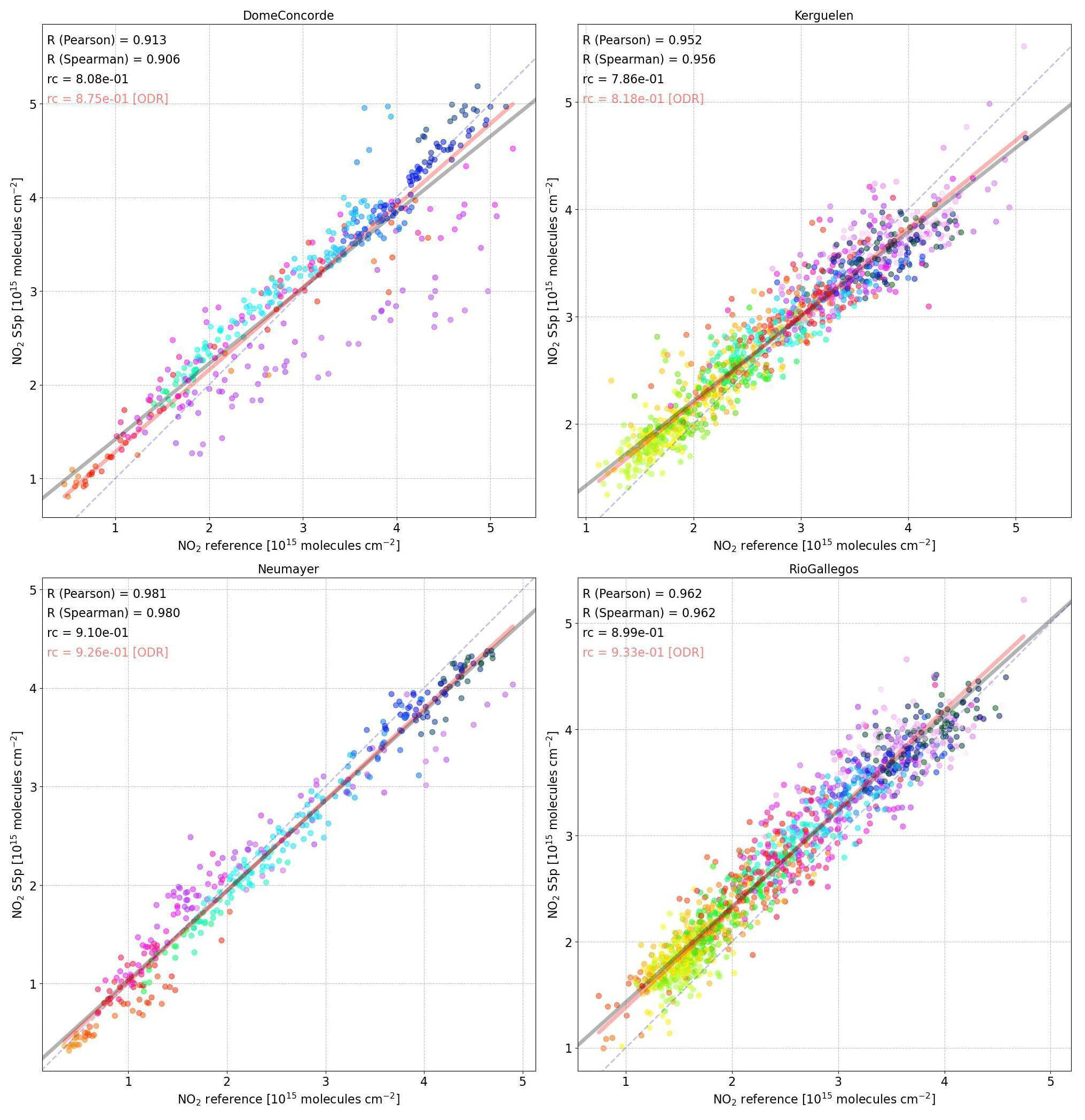
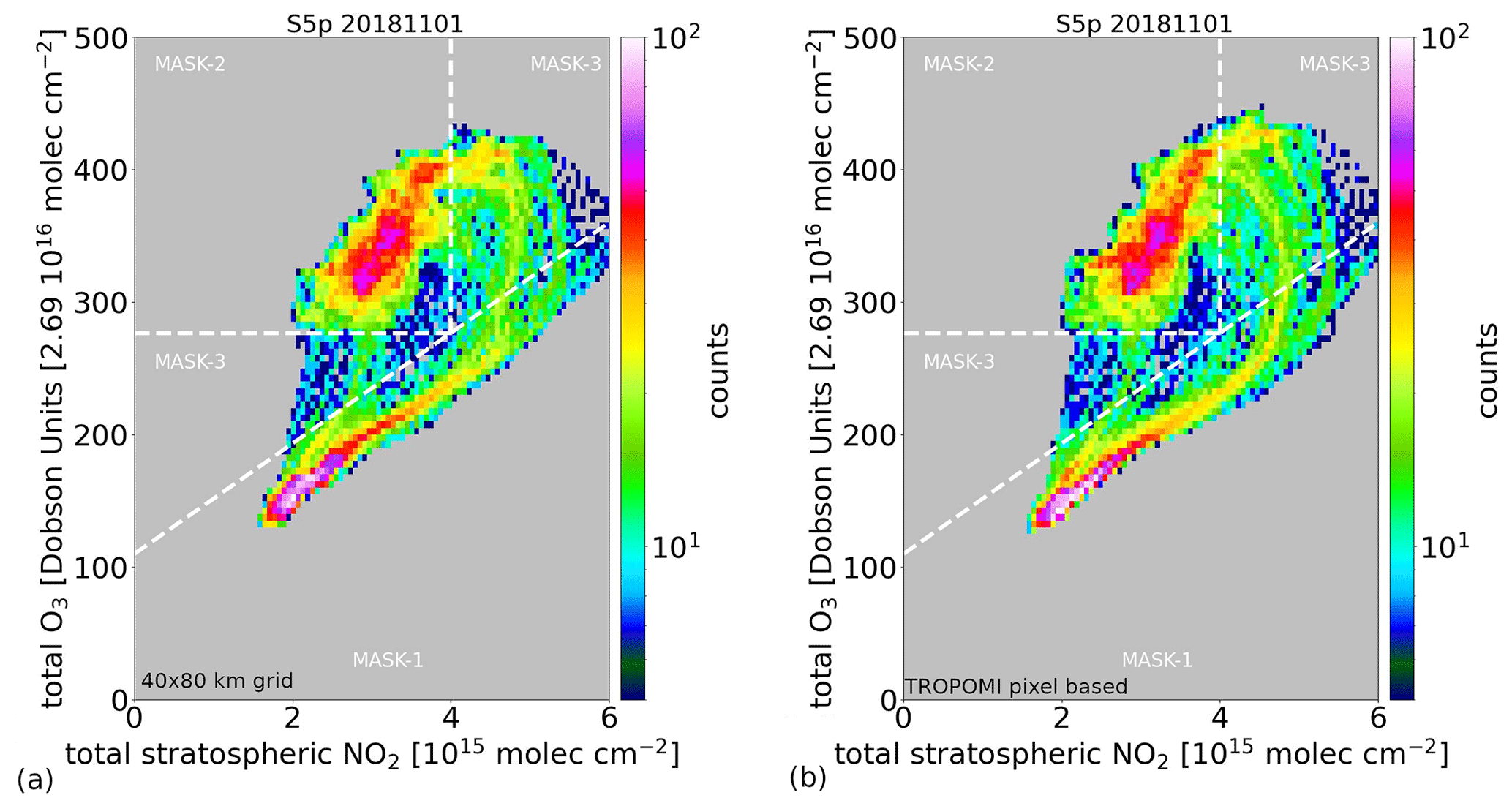
Figure A4 Comparison of 2D histograms of (a) TROPOMI SNO₂ data using the 40 × 80 km daily averages collocated with TCO₃ data (as Fig. 5a) and (b) TROPOMI SNO₂ pixel-level data collocated with TCO₃ data.