Effect of wind speed on marine aerosol optical properties over remote oceans with use of spaceborne lidar observations

Marine aerosol affects the global energy budget and regional weather. The production of marine aerosol is primarily driven by wind at the sea–air interface. Previous studies have explored the effects of wind on marine aerosol, mostly by examining the relationships between aerosol optical depth (AOD) and surface wind speed. In this paper, utilizing the synergy of aerosol and wind observations from Aeolus, the relationships between the marine aerosol optical properties at 355 nm and the instantaneous co-located wind speeds of remote oceans are investigated at two vertical layers (within and above the marine atmospheric boundary layer (MABL)). The results show that the enhancements of the extinction and backscatter coefficients caused by wind are larger within the MABL than above it. The correlation models between extinction and backscatter with wind speed were established using power-law functions. The slope variation points occur during extinction and backscatter coefficients increasing with wind speed, indicating that the wind-driven enhancement of marine aerosol involves two phases: a rapid-growth phase with high wind dependence, followed by a slower-growth phase after the slope variation points. We also compared the AOD–wind relationship acquired from Aeolus with CALIPSO-derived results from previous research. The variation in the lidar ratio with wind speed is examined, suggesting a possible “increasing–decreasing–increasing” trend of marine aerosol particle size as wind speed increases. This study enhances the comprehension of the correlation between marine aerosol optical properties and wind speed by providing vertical information and demonstrating that their relationships are more complex than a linear or exponential relation.

1 Introduction

According to the Intergovernmental Panel on Climate Change (IPCC) Fifth Assessment Report, the total emission of marine aerosol (including marine primary organic aerosol) produced from oceans is 1400–6800 Tg yr⁻¹, which is considered the largest natural aerosol input to the atmosphere globally (Boucher et al., 2013). Accurate estimations of marine aerosol production, evolution, and dissipation, as well as the knowledge of marine aerosol spatial and temporal distribution, are significant for studying the global energy budget, aerosol–cloud interactions and visibility changes (Latham and Smith, 1990; Murphy et al., 1998; O'Dowd et al., 1999; Haywood et al., 1999; de Leeuw et al., 2000; Kaufman et al., 2002; Smirnov et al., 2012). Radiative forcing caused by marine aerosol is a significant contributor to the global energy budget. It was reported that the average marine aerosol optical depth (AOD_mar) is approximately 0.15, while the volume concentration of cloud condensation nuclei from marine aerosol is around 60 cm⁻³ (Kaufman et al., 2002; Lewis and Schwartz, 2004). Therefore, marine aerosol has both direct and indirect impacts on radiative forcing by scattering and absorbing solar radiation and by modifying the microphysical properties of clouds, respectively (Murphy et al., 1998; Pierce and Adams, 2006). Knowledge of the impact of the magnitude of, and changes in, marine aerosol emissions on the shifts in climate and marine ecosystem processes is limited (IPCC, 2021).

Marine aerosol mainly includes primary sea spray particles and secondary aerosols produced by the oxidation of emitted precursors. Sea spray particles, composed of sea salt and primary organic aerosols, are produced by wind-induced wave breaking and the wind-driving direct mechanical disruption of wave crests (O'Dowd and de Leeuw, 2007; IPCC, 2021). Moreover, as a dynamical meteorological factor, wind speed also has vital influence on the transport, evolution, and dissipation of aerosols. Consequently, wind speed is a crucial factor which governs the production and life cycle of marine aerosol (Lewis and Schwartz, 2004). Exploring accurately the relationships between marine aerosol optical properties (aerosol optical depth (AOD), extinction coefficient (α), backscatter coefficient (β), etc.) and wind speed is significant for improving global aerosol transport models (Jaeglé et al., 2011; Madry et al., 2011; Fan and Toon, 2011), for enhancing satellite-retrieved AODs (Kahn et al., 2010; Kleidman et al., 2012), for atmospheric correction of ocean color (Zibordi et al., 2011), and for the study of biogeochemical cycles (Meskhidze and Nenes, 2010). Several efforts have been reported to investigate the relationship between the AOD or aerosol extinction coefficient over the ocean and wind speed. Utilizing either satellite-retrieved AODs (Glantz et al., 2009; Huang et al., 2010; Lehahn et al., 2010; O'Dowd et al., 2010; Grandey et al., 2011) or surface (coast, island, or ship)-based measurement AODs (Platt and Patterson, 1986; Villevalde et al., 1994; Smirnov et al., 1995; Wilson and Forgan, 2002; Smirnov et al., 2003; Shinozuka et al., 2004; Mulcahy et al., 2008; Lehahn et al., 2010; Adames et al., 2011; Sayer et al., 2012; Smirnov et al., 2012), most previous research focused on the AOD measured by passive instruments (mainly sun photometers). From these studies, various power-law or linear relationships have been established showing a positive correlation between AODs over the ocean and surface wind speed. However, passive instruments lack the ability to distinguish marine aerosol from other aerosols, to obtain vertical profiles of aerosols, and to retrieve aerosol optical properties in the absence of sunlight (except for lunar photometers) and under cloudy conditions (Kiliyanpilakkil and Meskhidze, 2011; Winker and Pelon, 2003). Active optical instruments for aerosol measurements, mainly lidar, were also used to reveal the relationship between AOD or the extinction coefficient of marine aerosol and wind speed. A shipborne depolarization lidar was occupied to acquire aerosol extinction coefficients over the East Sea of Korea near Busan and Pohang, associated with the wind measurement from an anemometer mounted on a mast, finding a positive linear relationship (R²=0.57) between extinction (532 nm) at 300 ± 50 m and wind speed at 20 m (Shin et al., 2014). However, this relationship was established using offshore data, and thus it can not be representative of the global ocean. The Cloud-Aerosol Lidar with Orthogonal Polarization (CALIOP) onboard the Cloud-Aerosol Lidar and Infrared Pathfinder Satellite Observation (CALIPSO) mission is capable of measuring the vertical distributions of global aerosol optical properties and identifying different aerosol types (including “clean marine”). Kiliyanpilakkil and Meskhidze (2011) selected CALIOP-retrieved pure AOD_mar below 2 km over the ocean utilizing the CALIOP aerosol subtype products and combined them with the surface wind speed provided by the Advanced Microwave Scanning Radiometer (AMSR-E) on board the Aqua satellite, acquiring a relatively complex increasing regression function, which will be presented and compared in Sect. 4.4.2. Furthermore, Prijith et al. (2014) also made use of CALIOP-retrieved AODs below 0.5 km over the ocean and the surface wind speed, obtaining nearly positive correlation linear relationships. Nevertheless, the assumed marine aerosol lidar ratio (LR_mar) (20 sr at 532 nm) was used in the AOD_mar retrieval process of CALIOP (Kiliyanpilakkil and Meskhidze, 2011), but the LR_mar can vary from 10 sr to around 40 sr at 532 nm (Groß et al., 2013, 2015; Bohlmann et al., 2018; Floutsi et al., 2023), which could generate deviations in the retrieval of AOD_mar. In summary, to explore accurately the relationship between marine aerosol optical properties and wind speed, it is essential to conduct global continuous observations and obtain the information of aerosol type identification, while vertical profiles of aerosols can provide extra spatial information for further analysis. Moreover, previous studies mostly focused on layer AOD_mar and ocean surface wind speed to explore the probable production of marine aerosol driven by surface wind. The relationship between the vertical optical properties of marine aerosol and the corresponding spatiotemporally synchronous wind speed, which represents the marine-atmospheric background state and may reveal the transport and evolution of marine aerosol vertically, remains to be investigated.

The Atmospheric Laser Doppler Instrument (ALADIN), the first-ever spaceborne direct detection wind lidar, which was launched into space in August 2018, was the unique payload installed on the Aeolus satellite mission of the European Space Agency (ESA) (Stoffelen et al., 2005; Reitebuch, 2012; Kanitz et al., 2019). As a direct detection high-spectral-resolution lidar, ALADIN was capable of providing the global aerosol optical property (e.g., α and β) profiles at 355 nm (Level-2A product), the horizontal-line-of-sight (HLOS) wind speed profiles (Level-2B product), and the wind vector profile from the European Centre for Medium-Range Weather Forecasts (ECMWF) model along the Aeolus track (Level-2C product) (Rennie et al., 2020). It should be emphasized that the aerosol and wind products are retrieved from the backscattered signal of the same laser light pulse emitted by ALADIN into the atmosphere, and hence the geolocation and time information of these products is completely consistent for each profile. The maximum detection height of these products is around 20 km and the vertical resolutions vary from 0.25 to 2 km (from bottom to top). Though regarded as a by-product, the particle optical property products have been demonstrated to provide valuable information about particles, especially on the detection and characterization of aerosol and cloud layers as well as on the lidar ratios (LRs) (Baars et al., 2021; Flament et al., 2021; Abril-Gago et al., 2022). Dai et al. (2022) conducted the first attempt on the combined application of the aerosol products (Level-2A products) and the wind vector products (Level-2C products) of ALADIN, observing an enormous dust transport event from the Sahara to the Americas in June 2020 and describing the transport quantitatively by calculating dust advection.

As mentioned above, Aeolus can provide global aerosol optical property profiles and wind speed profiles with high spatial and temporal resolution. Additionally, CALIOP can provide global aerosol type information. Hence, the combination of Aeolus–CALIOP products is capable of analyzing the relationship between marine aerosol optical properties (e.g., α, β, and LR) at 355 nm and wind speed globally and vertically. In this paper, utilizing the Aeolus Level-2A and Level-2C products together with the CALIOP aerosol subtype products, we (1) select ocean areas far from land and examine the dominance of marine aerosol over these areas using the CALIOP aerosol classification products; (2) attempt to acquire the pure marine aerosol optical properties (α, β, and LR) at 355 nm and the corresponding wind speeds from the Aeolus products, and to analyze the spatial distributions of these atmospheric state parameters at two separate vertical layers (0–1 km and 1–2 km, corresponding to the layers within and above the marine atmospheric boundary layer (MABL), respectively); and (3) investigate the relationship between the marine aerosol optical properties and the wind speeds vertically over the ocean. Generally, the highlights of this work mainly include (1) determining the spatiotemporally synchronous relationship between aerosol optical properties (α, β, and LR) and instantaneous wind speeds, which could indicate the background atmospheric states within and above the MABL over remote oceans, and (2) performing the analysis at two separate height layers above the ocean surface to explore the vertical differences in wind-driven marine aerosol evolution.

This paper is organized as follows: Sect. 2 introduces the spaceborne lidars and their specific products used in this study. Section 3 presents the methodology of study area selection, data pre-processing, and data analyses for relationship exploration between marine aerosol optical properties and wind speed. Section 4 presents the procedure of study area selection, then analyses and discusses marine aerosol optical properties, wind speed, and their relationship above three selected areas.

2 Spaceborne lidars and products

2.1 ALADIN

Since its launch in August 2018, ALADIN globally observed the profiles of the components of the wind vector along the laser's line of sight (LOS), and also the profiles of aerosol optical properties, for more than 4 years. Aeolus flew at a mean altitude of about 320 km in a sun-synchronous orbit with local Equator crossing times of about 06:00 and 18:00 LT, a daily quasi-global coverage (about 16 orbits per day), and an orbit repeat cycle of 1 week (111 orbits) (Reitebuch, 2012). Designed as a high-spectral-resolution lidar with a laser wavelength of 354.8 nm, ALADIN has the capability to simultaneously acquire wind profiles and particle optical properties with its two separate optical frequency discrimination channels named Rayleigh channel and Mie channel. Detailed descriptions of the instrument design and the measurement concept are introduced in, for example, Ansmann et al. (2007), Dabas et al. (2008), Flamant et al. (2008), Reitebuch (2012), Lux et al. (2020), and Flament et al. (2021).

Processed in different phases, the Aeolus data products are classified into several levels: Level 0 (instrument housekeeping data), Level 1B (engineering-corrected HLOS winds), Level 2A (aerosol and cloud layer optical properties), Level 2B (meteorologically representative HLOS winds) and Level 2C (Aeolus-assisted wind vectors) (Flamant et al., 2008; Tan et al., 2008; Rennie et al., 2020). It should be emphasized that Level-2C wind vectors are the output from the assimilation of the Aeolus Level-2B products in the ECMWF operational numerical weather prediction (NWP) model after 9 January 2020 (Rennie et al., 2021). In addition, the products of Aeolus are available in different baselines which correspond to different processor versions used to derive the products. The products were initially released as Baseline 07 and have been updated to Baseline 14 up to the time of this study (https://aeolus-ds.eo.esa.int/oads/access/; last access: 16 February 2023). As mentioned above, we use Level-2A and Level-2C products to study the relationship between marine aerosol optical properties and wind speed. Because Level-2C products can provide both components of the wind vector, we use Level-2C instead of Level-2B products from Aeolus. The time coverage of the Aeolus products used in this study is from 20 April 2020 to 4 July 2022. Thus, in terms of the Level-2A products used, the data processors are Baseline 11 (20 April 2020 to 26 May 2021), Baseline 12 (26 May 2021 to 6 December 2021), Baseline 13 (6 December 2021 to 29 March 2022), and Baseline 14 (29 March 2022 to 4 July 2022), while in terms of the Level-2C products, the data processors are Baseline 09 (20 April 2020 to 9 July 2020), Baseline 10 (9 July 2020 to 8 October 2020), Baseline 11 (8 October 2020 to 26 May 2021), Baseline 12 (26 May 2021 to 6 December 2021), Baseline 13 (6 December 2021 to 29 March 2022), and Baseline 14 (29 March 2022 to 4 July 2022), respectively (https://aeolus-ds.eo.esa.int/oads/access/; last access: 16 February 2023). The Level-2C NWP wind vector products from ECMWF used in this study are obtained after assimilation of the Level-2B observed HLOS wind products.

2.2 CALIOP

CALIOP, one of the payloads installed on CALIPSO, measured global vertical profiles of aerosol and cloud optical properties for more than 16 years starting in 2006. It can provide α at 532 and 1064 nm, β at 532 and 1064 nm, the depolarization ratio at 532 nm, vertical feature mask (VFM) products, and more. (Winker et al., 2009). The VFM products comprise the vertical information along each profile for cloud and aerosol identification, and further for the subtype classification of clouds and aerosols. For cloud and aerosol identification, the cloud–aerosol discrimination (CAD) algorithm was applied based on the layer-integrated volume depolarization ratio, layer-integrated total attenuated color ratio, and layer-averaged attenuated backscatter at 532 nm, as well as latitude and altitude (Liu et al., 2019). Aerosol subtypes are distinguished as “marine”, “dusty marine”, “dust”, “polluted dust”, “continental”, “polluted continental”, “elevated smoke”, and “others” via the joint analysis of the particulate depolarization ratio, integrated attenuated backscatter coefficient at 532 nm, layer top altitude, layer base altitude, and surface type (Kim et al., 2018). In this study, CALIOP Level (L2) VFM products are applied to confirm the dominance of the marine aerosol over the selected ocean areas. Different versions of the CALIOP L2 VFM product are used, namely 4.10 (20 April 2020 to 1 July 2020), 4.20 (1 July 2020 to 19 January 2022), and 3.41 (19 January 2022 to 4 July 2022).

3 Methodology

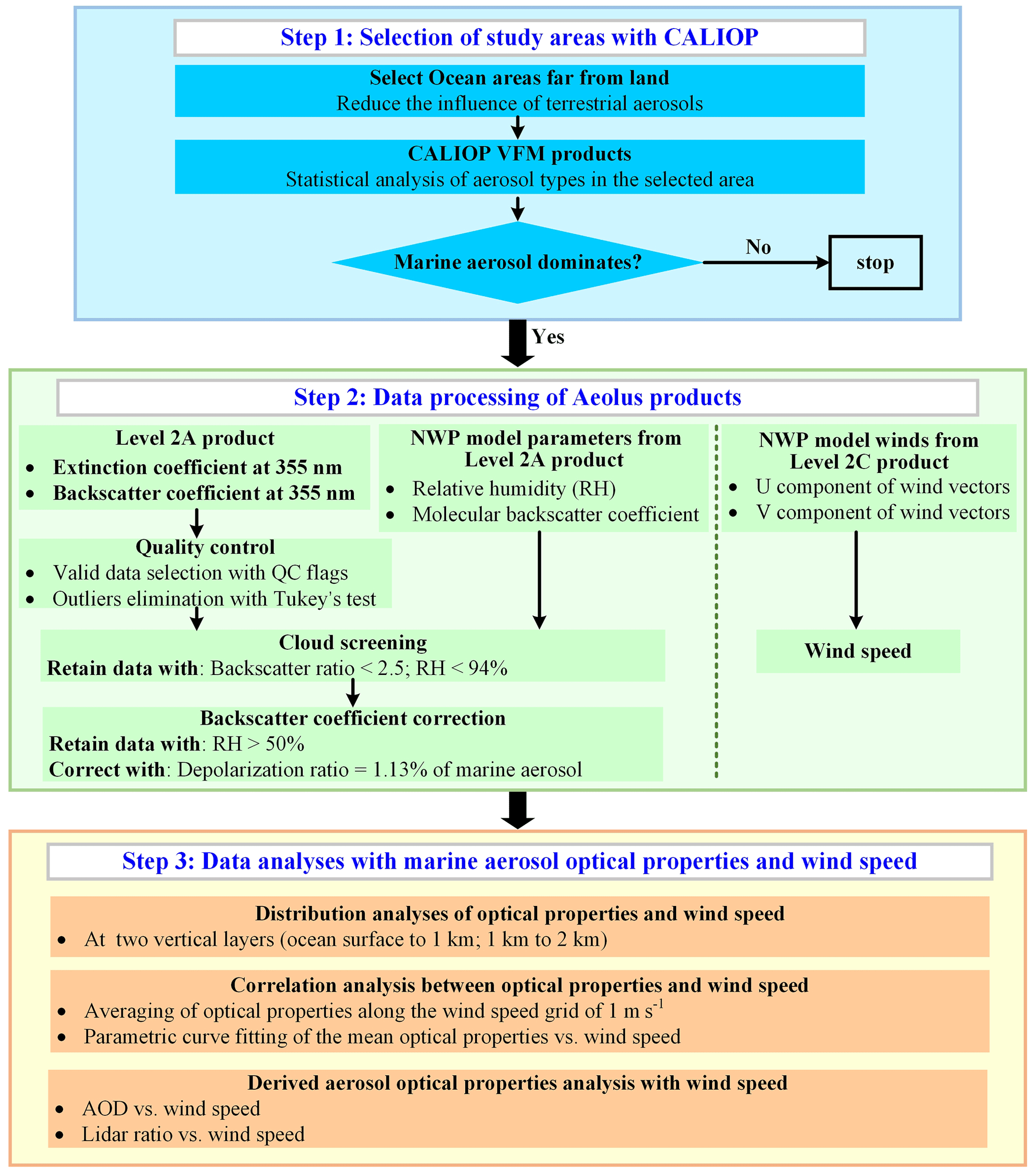
In general, the data processing and analysis procedure of this study can be summarized briefly in three parts, including the selection of the study areas, data pre-processing, and data analyses.

This work mainly focuses on marine aerosol, and hence the ocean areas for the study are supposed to be far away from land to reduce the influence of terrestrial aerosols, e.g., anthropogenic activities, dust, and biomass burning. In this work, we selected three ocean areas located in the North Pacific (NP), South Pacific (SP), and South Indian (SI) oceans, with the latitude and longitude ranges of 0–30° N and 150° E–150° W , 20–60° S and 100–150° W, as well as 20–60° S and 60–90° E, respectively, as shown in Fig. 1. Therefore, in this paper, we refer to these three remote ocean areas as “the NP area”, “the SP area”, and “the SI area”, respectively.

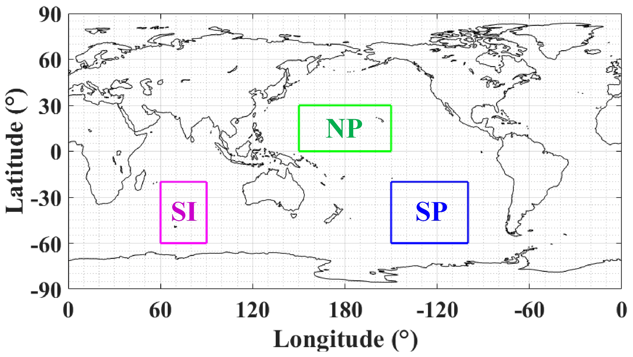
Figure 1 The selected ocean study areas.

The aerosol classification information from the CALIOP VFM products is utilized to statistically analyze the aerosol types of the selected areas. It is found that marine aerosol is mostly distributed in the altitude range of 0–2 km during VFM processing. Therefore, the statistical analysis of the aerosol types is conducted in the same altitude range. Marine aerosol is considered to dominate in the selected area if the percentage of the aerosol subtype “marine” is larger than 75 % while the percentage sum of “marine” and “dusty marine” is above 90 %; if so, then the study can be continued for this area.

The α at 355 nm and β at 355 nm retrieved by the standard correction algorithm (SCA) from the Aeolus Level-2A product are used in this study, as the SCA processing is capable of producing more stable α and β than the Mie channel algorithm (Flament et al., 2021). Furthermore, the mid-bin product (sca_optical_properties_mid_bins) of the SCA product is chosen because the mid-bin algorithm is more robust (Baars et al., 2021; Flament et al., 2021). To ensure high data quality for the study of the relationship between the optical properties and wind speed, a rigorous quality control has to be applied. In the aspect of quality control, negative α and β are excluded, and then the quality flags (“bin_1_clear” and “processing_qc_flag”) provided in the Level-2A product are applied to filter out invalid data (Trapon et al., 2022). Additionally, the outliers are labeled and eliminated by the boxplot analysis. Using the lower quartiles Q_L (25 % positions of the data) and the upper quartiles Q_U (75 % positions of the data), this method classifies the data below $Q_{\mathrm{L}}-\mathrm{3}\cdot \left(Q_{\mathrm{U}}-Q_{\mathrm{L}}\right)$ or above $Q_{\mathrm{L}}+\mathrm{3}\cdot \left(Q_{\mathrm{U}}-Q_{\mathrm{L}}\right)$ as outliers (Hoaglin et al., 1986). The Aeolus products do not differentiate between aerosol and cloud, which means that the particle optical properties of a single data bin may contain a mixture of both types of information. Aeolus-measured particulate β, combined with relative humidity (RH) and molecular β from the ECMWF NWP model provided in the Level-2A product, is utilized to screen the cloud layers. A cloud is considered quite likely to be present if the backscatter ratio (BR) (total backscatter coefficient divided by molecular backscatter coefficient) at 355 nm is larger than 2.5 or the RH is larger than 94 % (Flamant et al., 2020). Therefore, in this study, if the BR is larger than 2.5 or the RH is higher than 94 %, the corresponding data bin is considered to be cloud contaminated and is eliminated. With this cloud screening approach, in this study, 9 %, 35 %, and 40 % of the data in the altitude range of 0–2 km were eliminated for the NP area, the SP area, and the SI area, respectively. Due to the instrument design of ALADIN, it can only detect the co-polar backscattered light, leading to the lack of the depolarized portion of the β (Flamant et al., 2020). According to Groß et al. (2015), the depolarization ratio at 355 nm of marine aerosol (δ_mar,355 nm) is approximately 0.02 when the RH is larger than 50 %. Nevertheless, dried marine aerosol layers can significantly depolarize with the depolarization ratios varying from 0.02 to around 0.1, making the typical δ_mar,355 nm of humid marine aerosol (RH>50 %) unsuitable for dried aerosol (Haarig et al., 2017; Bohlmann et al., 2018). Consequently, to correct the marine aerosol backscatter coefficient with the typical δ_mar,355 nm of humid marine aerosol, the data with RH>50 % are retained (around 95 % of the data are retained), and thus with the typical δ_mar,355 nm the total marine aerosol backscatter coefficient β_mar can be calculated by Eq. (1):

$$\begin{array}{}\text{(1)}& {\mathit{\beta }}_{\text{mar}}=(\mathrm{1}+{\mathit{\delta }}_{\text{mar,355\hspace{0.17em}nm}})\cdot {\mathit{\beta }}_{\text{mar,Aeolus-co}},\end{array}$$

where β_{mar,Aeolus-co} is the original marine aerosol backscatter coefficient measured by ALADIN. It should be noted that all the aerosol β values from Aeolus identified as β_{mar,Aeolus-co} values and then utilized to calculate β_mar values by Eq. (1) are under the ideal assumption that marine aerosol is the only aerosol type in the study areas. Though the study areas are all located in remote oceans far away from land and are evaluated as “marine aerosol dominates” by CALIOP, there are a few terrestrial aerosols like dust, polluted dust, polluted continental, and smoke, with a total proportion of no more than 10 % (see Sect. 4.1 for details). For terrestrial aerosols, the depolarization ratios at 355 nm are 0.22–0.24 for dust, 0.16 for polluted dust, 0.01 for polluted continental, and 0.03 for smoke, among which those for dust and polluted dust are much larger than δ_mar,355 nm (Floutsi et al., 2023). Consequently, regarding all the aerosols as marine aerosol and correcting β_mar according to Eq. (1) leads to an obvious underestimation in the β for dust and polluted dust. Nevertheless, in view of the small proportions of dust (maximum 3.15 %) and polluted dust (maximum 0.79 %) above the study areas, and thanks to the statistical analyses of the data for a long period, the assumption that all aerosols are considered as marine aerosol does not critically impact the β_mar–wind speed relationship, although it should be noted that the actual β is a little bit larger than the β_mar.

As for the wind vector data, the Aeolus Level-2C product provides the u component (zonal components of the wind vector) and the v component (meridional components of the wind vector) from the ECMWF model after assimilation of the Level-2B observational wind product, in the same data bins of the Level-2A optical properties product. Hence, the wind speed (ws) can be calculated with these two components by Eq. (2):

$$\begin{array}{}\text{(2)}& \text{ws}=\sqrt{u^{\mathrm{2}}+v^{\mathrm{2}}}.\end{array}$$

With the reprocessed marine aerosol optical properties extinction coefficient α_mar and β_mar, and the corresponding wind speed, it is possible to explore the relationship between these parameters. At the beginning of the data analyses, α_mar, β_mar, and wind speed within the altitude range of 0–2 km are selected, where marine aerosol dominates according to the analysis of CALIOP VFM. Furthermore, the whole study height range is divided into two individual layers. Referring to the results of Luo et al. (2014, 2016) and Alexander and Protat (2019), the MABL height of remote oceans is summarized to be around 1 km. Moreover, calculated with ECMWF-provided boundary layer heights at the three study areas for the time period of 20 April 2020 to 26 May 2021, the mean values and the standard deviations are 787.47 ± 231.77 m at the NP area, 939.39 ± 360.20 m at the SP area, and 1005.29 ± 366.60 m at the SI area. Hence, the boundary height of the two vertical layers is set at 1 km, which is approximately the mean MABL height of remote oceans. Though the MABL heights are variable and therefore setting 1 km will lead to potential inaccuracies, the relatively low height resolution of Aeolus (0.25 km below 0.5 km, 0.5 km in the altitude of 0.5–2 km) limits the use of more precise height boundaries. The statistical results of the 0–1 km layers and the 1–2 km layers are considered generally representative of the atmospheric conditions within the MABL and above the MABL. In this paper, the lower layer with the altitude range of 0–1 km is called Layer_L and the higher layer with the altitude range of 1–2 km is called Layer_H. It is important to note that the lowest altitude bins of Aeolus observation products may contain the reflections from the surface or even be subsurface, and thus they are contaminated and not representative of the atmospheric wind speed and the aerosol optical properties (Wu et al., 2022). Regarding the ocean applications of spaceborne lidar observations, it is known that the lidar attenuated backscatter coefficients of the bin containing the ocean surface can be affected by the processes at the surface of the ocean, namely, stronger winds resulting in weaker backscattering (Josset et al., 2008). Labzovskii et al. (2023) indicated that Aeolus return signals are unlikely sensitive to ocean surface dynamical conditions (related to wind), which makes the analysis of marine aerosol optical properties in the MABL free from adverse effects stemming from the ocean surface. Nevertheless, during the data processing, it was discovered that all data (Level-2A particle optical properties and Level-2C wind vectors) below 0.25 km, which could be contaminated by reflections from the land or ocean surface, were screened out using Aeolus quality control flags, and then the lowest data bins were at around 0.25 km. This may indicate that the actual altitude range of marine aerosol optical properties in Layer_L is around 0.25–1 km. Although the data near the sea–air interface are missing, all available data avoid the contamination of the ground return signals and eliminate the risk of being affected by ocean surface dynamical conditions. Over the selected ocean areas, the spatial distributions of the α_mar, β_mar, and wind speed are acquired with the longitude–latitude grid of 5°×5° at two separate layers. Then the relationship analyses between the optical properties (α_mar and β_mar) and wind speed of these two layers are conducted by averaging the optical properties along wind speed grids (1 m s⁻¹) and by parametric curve fitting. For the average calculations, specifically, a grid with a resolution of 1 m s⁻¹ from 0 to 30 m s⁻¹ is defined and the mean values as well as the standard deviations along the grid are calculated for both layers above the study areas, respectively. It should be emphasized primarily that before calculating the averages of each wind speed grid, the outliers larger or less than the average ± 1 standard deviation are eliminated. About 70 %–80 % of α_mar and β_mar are retained after the elimination. The rather strict outlier removal is conducted here to reject the data that are not representative of marine aerosol (i.e., may be contaminated by clouds, thus becoming higher than the typical range). Hence, it can guarantee the data quality and the validity of the pure marine aerosol optical properties in the statistical analysis process. Moreover, the wind speed grid with data counts less than 100 is considered unrepresentative and the statistical result of this grid is discarded. As derived data of α_mar, β_mar, averaged AOD_mar, and LR_mar are obtained and discussed as well. The AOD_mar is acquired by integrating Aeolus-retrieved α_mar within 2 km of each single profile. The AOD_mar is calculated within the height of 2 km in order to compare it with the previous result of CALIOP, where the integration height is the same as that in this study. In Sect. 4.4.1, the averaged AOD_mar along the wind speed grid is obtained and then compared with the AOD_mar–wind speed relationships from a previous study. The LR_mar is derived via dividing α_mar by β_mar for each corresponding data bin. The spatial distribution of LR_mar is presented in Sect. 4.2, while the relationships between the variations in LR_mar along wind speed grids and the marine aerosol particle size are discussed in Sect. 4.4.2.

The procedures of the study methodology are summarized in a flowchart in Fig. 2.

Figure 2 Flowchart of the study methodology.

4 Results and discussion

4.1 Analysis of aerosol types

To verify the dominance of marine aerosol, as discussed in Sect. 3, the CALIOP VFM aerosol classification products are applied. The proportions of eight aerosol types (marine, dusty marine, dust, polluted dust, continental, polluted continental, smoke, and others) are counted in two vertical layers defined in Sect. 3 over the NP area, the SP area, and the SI area, respectively, as shown in the histograms in Fig. 3. The proportions of marine aerosol at Layer_L in these three separate areas are 87 %, 84 %, and 84 %, while the proportions at Layer_H are 84 %, 79 %, and 79 %, respectively, which are all larger than 75 %. Moreover, the sums of the percentage of marine aerosol and dusty marine aerosol are all above 90 % for both layers and for all study areas. Consequently, the selected areas NP, SP, and SI can be considered as the marine aerosol dominating areas. It should be noted that “dusty marine”, an aerosol subtype introduced for the first time in version 4.10 of the CALIOP VFM product, was not present in version 3.41 and was identified from part of the “polluted dust” of version 3.41 with the criteria of “surface type” and “layer base altitude”. The use of version 3.41 of the CALIOP VFM data for the period from 19 January 2022 to 4 July 2022 led to the underestimation of the “dusty marine” fraction and the total marine aerosol fraction. Even though, under the condition of underestimation, the percentage of total marine aerosol is larger than 90 %, which means that the real proportion of total marine aerosol is higher, the conclusion that marine aerosol dominates in the altitude range of 0–2 km above these three areas is still valid.

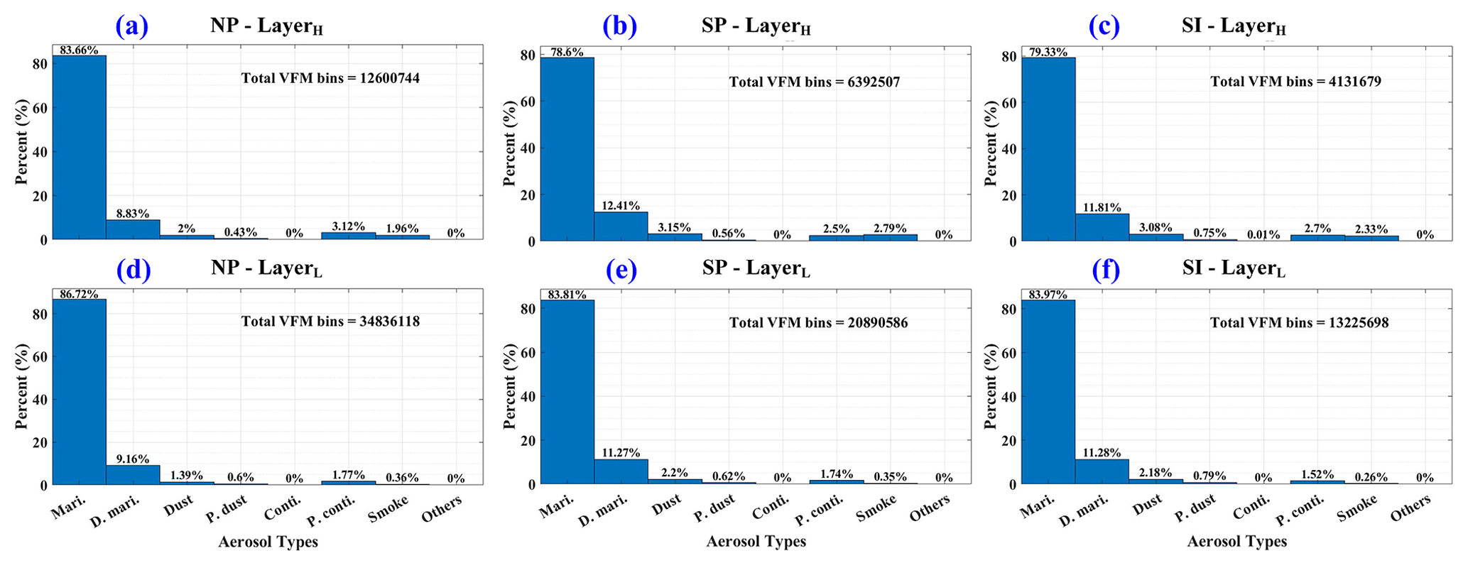
Figure 3 Statistical analyses of aerosol types over the NP area (a, d), the SP area (b, e), and the SI area (c, f) at two separate layers.

In this section, with the statistical analyses of aerosol types, the dominance of marine aerosol is confirmed in these three areas. It should be noted that among the areas, the NP area is mainly located at low latitudes or in the tropics, while the SP area and the SI area are located in mid-latitude regions.

4.2 Spatial distribution of wind speed and aerosol optical properties

With the Aeolus Level-2A product (particle optical properties) and Level-2C product (ECMWF model winds) from April 2020 to July 2022, calculated for each 5°×5° grid, the averaged wind speed, α_mar, β_mar, and LR_mar spatial distributions of Layer_H and Layer_L are acquired.

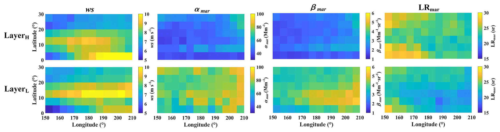
Figure 4 Wind speed (ws), marine aerosol extinction coefficient (α_mar), marine aerosol backscatter coefficient (β_mar), and marine aerosol lidar ratio (LR_mar) spatial distributions above the North Pacific (NP) area at Layer_H and Layer_L.

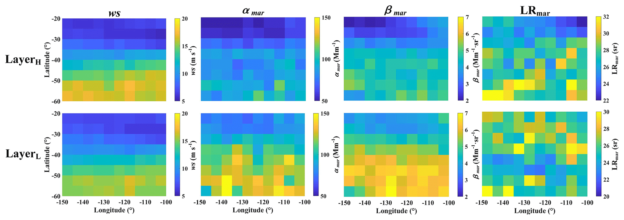
Figure 5 Wind speed (ws), marine aerosol extinction coefficient (α_mar), marine aerosol backscatter coefficient (β_mar), and marine aerosol lidar ratio (LR_mar) spatial distributions above the South Pacific (SP) area at Layer_H and Layer_L.

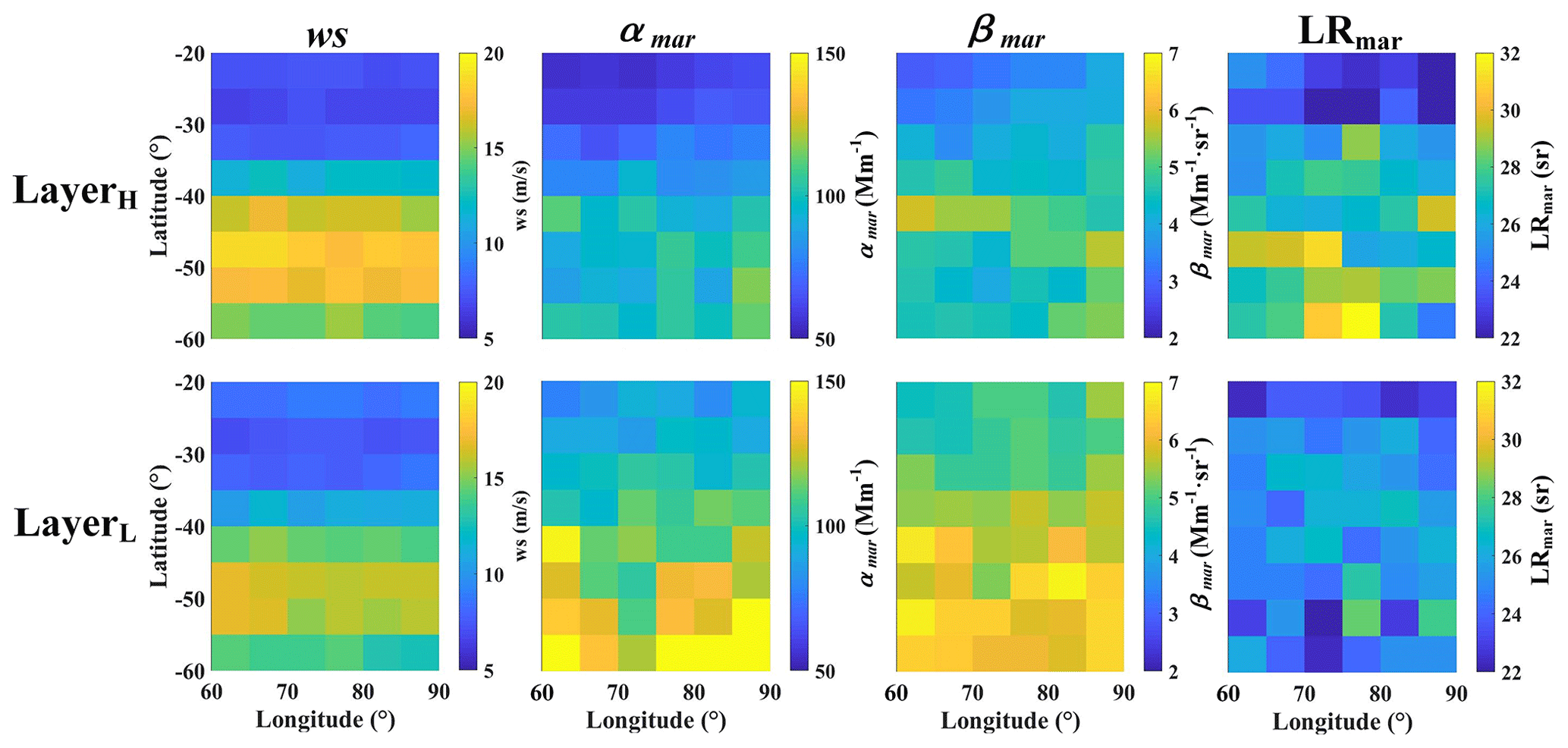
Figure 6 Wind speed (ws), marine aerosol extinction coefficient (α_mar), marine aerosol backscatter coefficient (β_mar), and lidar ratio (LR_mar) spatial distributions above the South Indian (SI) area at Layer_H and Layer_L.

Figures 4–6 present the averaged spatial distributions of atmospheric parameters at two layers above the NP area, the SP area, and the SI area. These figures describe the atmospheric background state of optical properties and wind speed within (Layer_L) and above (Layer_H) the MABL over the study areas. Primarily, the spatial variations in wind speed, α_mar, and β_mar are more apparent along the meridian than zonally, both at Layer_H and at Layer_L. In the aspect of Layer_L, there are separate distinct high wind speed regions or belts along the latitude in the three areas, which are the 5–20° N region of the NP area with the wind speed bins from approximately 8 m s⁻¹ to more than 10 m s⁻¹, the 40–60° S region of the SP area with the wind speed bins from more than 10 m s⁻¹ to approximately 17 m s⁻¹, and the 35–60° S region of the SI area with the wind speed bins from more than 10 m s⁻¹ to approximately 17 m s⁻¹ as well. Inspection of marine aerosol optical properties, α_mar, and β_mar in the high wind speed regions are obviously larger than in other regions. Hence, it can be inferred that, in the MABL, the wind speed and the marine aerosol optical properties tend to be positively correlated. Referring to Layer_H, shown in the upper four panels of Figs. 4–6, it can be seen that the spatial variation trends of wind speed, α_mar, and β_mar in the three areas are similar to those at Layer_L. The apparent high wind speed regions, where the wind speeds are up to around 8–10 m s⁻¹ in 5–20° N of the NP area, 15–18 m s⁻¹ in 40–60° S of the SP area, and 13–19 m s⁻¹ in 35–60° S of the SI area, also exist at Layer_H, while α_mar and β_mar are slightly enhanced in these regions which indicates that the wind speed may still have a weak positive influence on the marine aerosol optical properties at the higher atmospheric layer above the MABL. Some differences in the spatial distribution of wind speed, α_mar, and β_mar between the three areas can be discovered as well. As for the SP area and the SI area, wind speed, α_mar, and β_mar all mainly present increasing tendencies from north to south. In terms of the NP area, besides the obvious enhancements of wind speed, α_mar, and β_mar in the high wind speed belt, the gradual enhancements of these atmospheric parameters from west to east are presented in this area.

At both layers of the NP area and at Layer_L of the SP area, the LR_mar turns out lower in the relatively high wind speed regions, which illustrates a possible negative correlation between LR_mar and wind speed. The relationship between these two parameters is analyzed and discussed in detail in Sect. 4.4.2.

Additionally, the mean values and the standard deviations of these atmospheric parameters at Layer_H and Layer_L are calculated for each study area by averaging the spatial distributions of the 5°×5° grid, and are presented in Fig. 7. The averaged wind speed values are 8.1 ± 1.0, 11.1 ± 3.5, and 12.0 ± 3.5 m s⁻¹ at Layer_L, while 7.9 ± 1.1, 11.5 ± 4.2, and 12.5 ± 4.5 m s⁻¹ at Layer_H, above the NP area, the SP area, and the SI area, respectively. The averaged α_mar values are 76 ± 7, 107 ± 22, 113 ± 22 Mm⁻¹ at Layer_L, while 47 ± 7, 78 ± 16, 84 ± 18 Mm⁻¹ at Layer_H, above the NP area, the SP area, and the SI area, respectively. The averaged β_mar values are 4.1 ± 0.5, 5.3 ± 1.7, and 5.6 ± 0.7 ${\mathrm{Mm}}^{-\mathrm{1}}{\mathrm{sr}}^{-\mathrm{1}}$ at Layer_L, while 2.2 ± 0.4, 4.0 ± 0.9, and 4.4 ± 0.7 ${\mathrm{Mm}}^{-\mathrm{1}}{\mathrm{sr}}^{-\mathrm{1}}$ at Layer_H, above the NP area, the SP area, and the SI area, respectively. The averaged LR_mar values are 22.3 ± 1.6, 25.9 ± 1.8, and 25.0 ± 1.5 sr at Layer_L, while 24.5 ± 1.6, 27.3 ± 2.3, and 26.3 ± 2.7 sr at Layer_H, above the NP area, the SP area, and the SI area, respectively. It is reported that the typical ranges of α_mar and β_mar at 532 nm over remote ocean areas are around 60–80 Mm⁻¹ and around 1–5 ${\mathrm{Mm}}^{-\mathrm{1}}{\mathrm{sr}}^{-\mathrm{1}}$, respectively, as observed and retrieved by CALIOP (Prijith et al., 2014; Kiliyanpilakkil and Meskhidze, 2011). Applying the typical α_mar Ångström exponent from 532 to 355 nm of 0.7 ± 1.3 and the typical β_mar Ångström exponent from 532 to 355 nm of 0.8 ± 0.1 (Floutsi et al., 2023), the converted typical ranges of α_mar and β_mar at 355 nm can be calculated, which are around 47–180 Mm⁻¹ and around 1.3–7.2 ${\mathrm{Mm}}^{-\mathrm{1}}{\mathrm{sr}}^{-\mathrm{1}}$. Compared with the typical ranges of α_mar and β_mar at 355 nm, calculated from CALIOP-retrieved typical ranges of marine aerosol optical properties and the typical conversion coefficients, the Aeolus-retrieved α_mar and β_mar are considered reasonable. The mean values of wind speed, α_mar, and β_mar above the NP area are the lowest among the three areas, both at Layer_H and Layer_L, which may be because that area is located in the low latitude region of the Northern Hemisphere. The highest mean wind speed of the SI area corresponds to the highest α_mar and β_mar. The mean wind speeds of Layer_H are both larger than those of Layer_L in the SP area and in the SI area, while the phenomenon is opposite in the NP area. It is worth noting that in all the study areas, the averaged α_mar and β_mar at Layer_L are larger than those at Layer_H, illustrating that the majority of the aerosol from oceans is trapped in the MABL, while a fraction of the marine aerosol can be elevated above the MABL. In terms of the averaged LR_mar, the values at Layer_H are all higher than those at Layer_L, and all the values are within a reasonable range with reference to those reported by Bohlmann et al. (2018), Groß et al. (2011, 2015), and Floutsi et al. (2023).

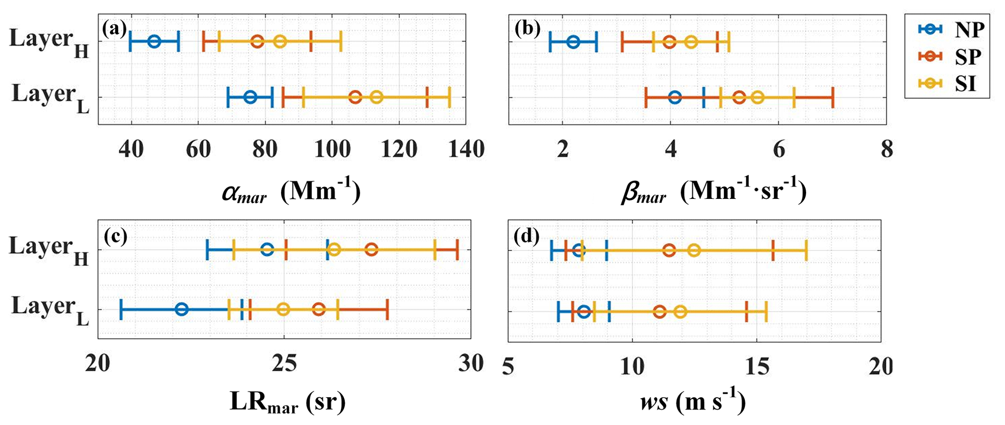
Figure 7 Mean values at Layer_H and Layer_L of (a) marine aerosol extinction coefficient (α_mar), (b) marine aerosol backscatter coefficient (β_mar), (c) marine aerosol lidar ratio (LR_mar), and (d) wind speed (ws) above the North Pacific (NP) area (blue standard deviation bars), the South Pacific (SP) area (red standard deviation bars), and the South Indian (SI) area (yellow standard deviation bars).

In conclusion, this section presents the atmospheric background state of optical properties and wind speed, as well as analyzes the spatial distributions of wind speed, α_mar, and β_mar jointly at Layer_H and Layer_L, above the NP area, the SP area, and the SI area, respectively. The α_mar and β_mar retrieved from Aeolus Level-2A products are in reasonable agreement with CALIOP, and the Aeolus-derived LR_mar values are also reasonable. It is found that, both at Layer_H and at Layer_L, spatially, the wind speed, α_mar, and β_mar show positive correlation, though the optical properties at Layer_L are greater than those at Layer_H indicating that both layers receive the input of the aerosol produced from the ocean by the wind but the majority of the marine aerosol is trapped in the MABL and only a small fraction can be elevated into the higher layer. In addition, as the three study areas are located in different regions, the spatial distributions of wind speed, α_mar, and β_mar are different.

4.3 Relationship between marine aerosol optical properties and wind speed

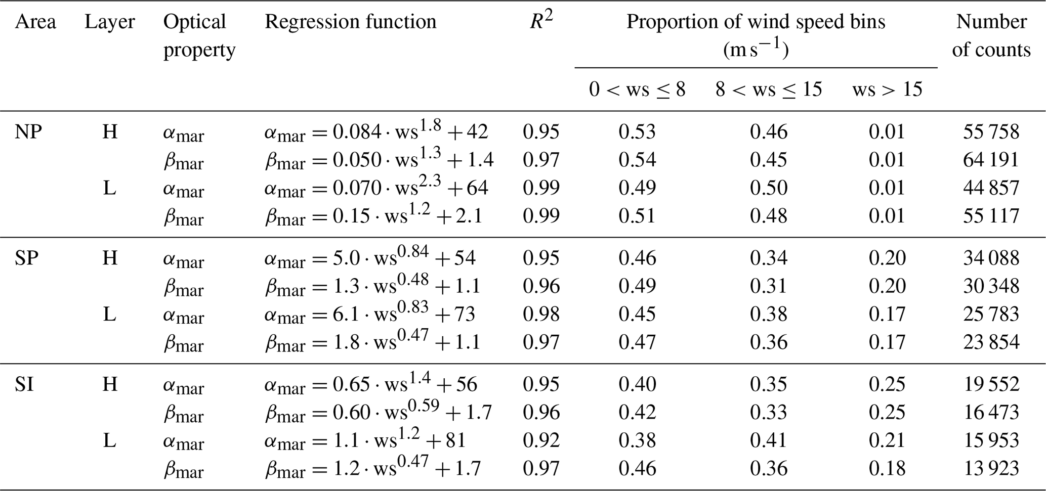
In order to determine the relationship between the marine aerosol optical properties and the corresponding wind speed, utilizing the method introduced in Sect. 3, the mean values and standard deviations (after outlier removal) of α_mar and β_mar, along with the wind speed grid at two layers above the NP area, the SP area, and the SI area, are shown in panels (a) and (b) of Figs. 8–10, respectively. The regression curves of the optical properties are presented in these figures as well. The power-law function is used for curve fitting to describe the trend of marine aerosol optical properties with wind speed. In addition, the data counts in each wind speed grid are shown as the histograms in panels (a) and (b) of Figs. 8–10. In order to illustrate the variation tendencies of α_mar and β_mar, the slopes of α_mar and β_mar with wind speed are also provided in panels (c) and (d) of Figs. 8–10. Table 1 summarizes the regression functions together with the corresponding R², and the proportions of the different wind speed bins together with the count sums, grouped by area, layer, and optical property.

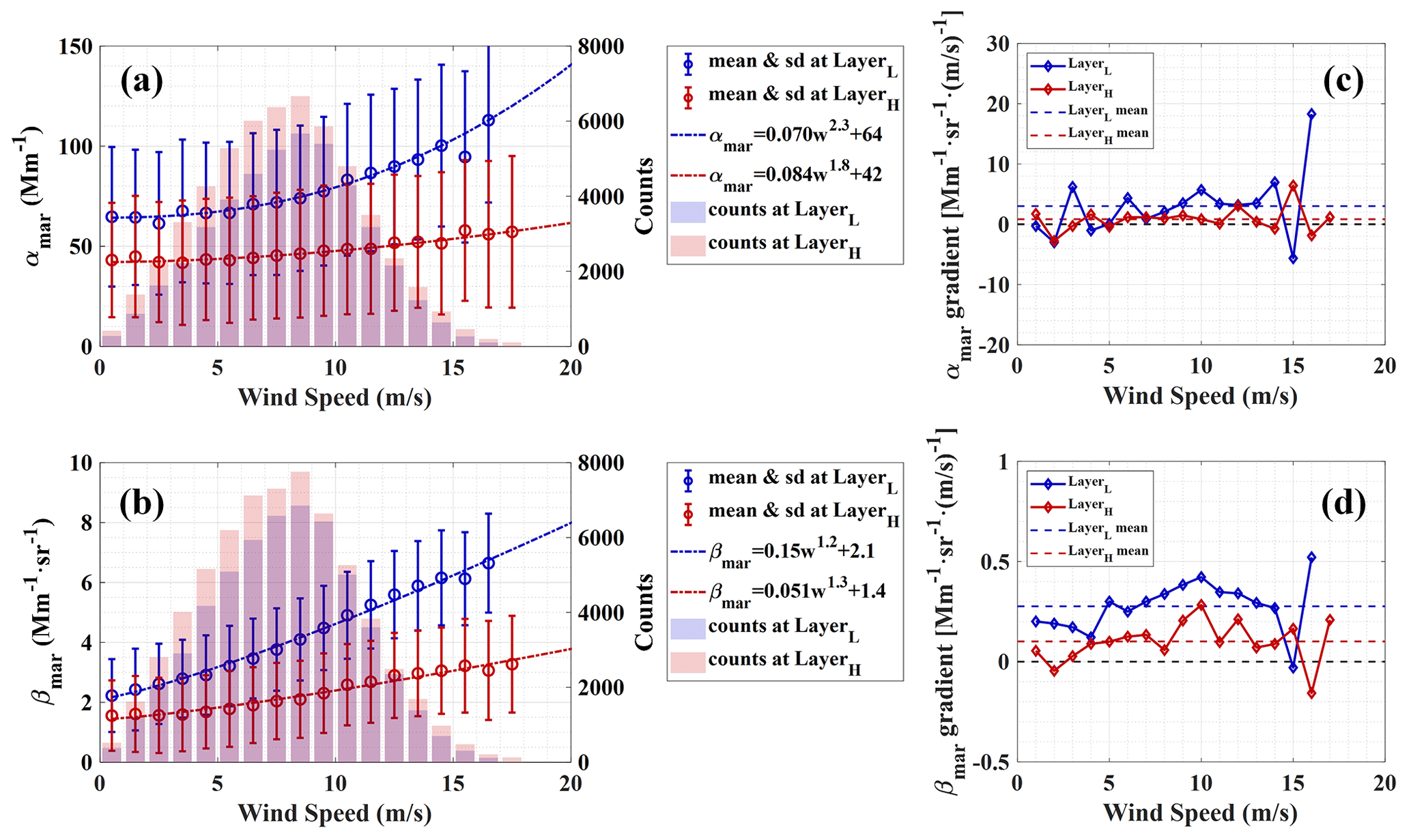
Figure 8 Relationship between marine aerosol optical properties ((a) for α_mar and (b) for β_mar) and wind speed above the NP area. The blue circles and error bars represent the means and standard deviations of the optical properties along wind speed grids at Layer_L, while the reds represent the same items at Layer_H. The dotted–dashed blue and red lines are the optical property average regression curves fitted along the wind speed grid at Layer_L and Layer_H, respectively. The blue and red histograms indicate the data counts of every wind speed grid at Layer_L and Layer_H, respectively. Panels (c) and (d) represent the slopes of α_mar and β_mar with wind speed at Layer_L (blue lines) and Layer_H (red lines), respectively, while the dashed blue lines and the dashed red lines show the mean values of the slopes at two layers.

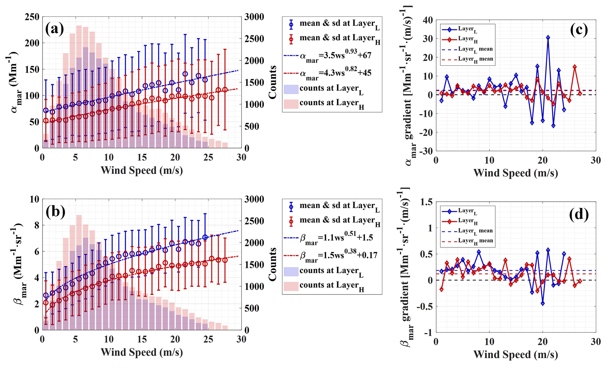
Figure 9 Relationship between marine aerosol optical properties and wind speed above the SP area. The items represent the same as those of Fig. 8.

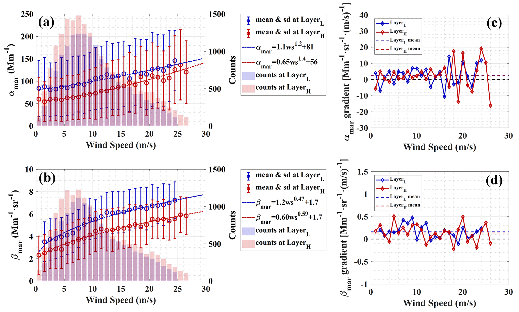
Figure 10 Relationship between marine aerosol optical properties and wind speed above the SI area. The items represent the same as those of Fig. 8.

Table 1 Regression functions of the averaged optical properties and the wind speed grids, together with the corresponding wind speed distributions, grouped by area and layer.

From the statistical results with wind speed grids and wind speed ranges, it can be found that most of the wind speeds are below 15 m s⁻¹ above the NP area, both at Layer_H and Layer_L, while the proportion of low wind speed ($\mathrm{0}<\text{ws}\le \mathrm{8}$ m s⁻¹) is slightly higher at Layer_H than at Layer_L. As for the SP area and the SI area, the proportions of high wind speed (ws>15 m s⁻¹) account for around one-fifth to one-quarter, respectively, and the proportion of low wind speed over the SP area is higher than that over the SI area. The wind speed distribution is more concentrated at Layer_L than at Layer_H above these two areas, in view of the lower proportion of low and high wind speeds and the higher proportion of medium wind speeds ($\mathrm{8}<\text{ws}\le \mathrm{15}$ m s⁻¹) at Layer_L.

Generally, in all cases shown in Figs. 8–10, the optical properties at Layer_L are all larger than those at Layer_H in the same wind speed grid, while with the variations in the marine aerosol optical properties along the wind speed grid it can be clearly observed that the tendency is increasing with the wind speed. Moreover, the regression curves are fitted pretty well as the R² are all above 0.90.

As Fig. 8a and b show, in the NP area, α_mar at Layer_L increases from 64 Mm⁻¹ at the 0–1 m s⁻¹ wind speed interval to 113 Mm⁻¹ at the 16–17 m s⁻¹ wind speed interval, while at Layer_H it increases from 42 Mm⁻¹ at the 0–1 m s⁻¹ wind speed interval to 57 Mm⁻¹ at the 17–18 m s⁻¹ wind speed interval; β_mar at Layer_L increases from 2.2 ${\mathrm{Mm}}^{-\mathrm{1}}{\mathrm{sr}}^{-\mathrm{1}}$ at the 0–1 m s⁻¹ wind speed interval to 6.6 ${\mathrm{Mm}}^{-\mathrm{1}}{\mathrm{sr}}^{-\mathrm{1}}$ at the 16–17 m s⁻¹ wind speed interval, while at Layer_H it increases from 1.6 ${\mathrm{Mm}}^{-\mathrm{1}}{\mathrm{sr}}^{-\mathrm{1}}$ at the 0–1 m s⁻¹ wind speed interval to 3.3 ${\mathrm{Mm}}^{-\mathrm{1}}{\mathrm{sr}}^{-\mathrm{1}}$ at the 17–18 m s⁻¹ wind speed interval. The increments of these two parameters at Layer_L are much larger than those at Layer_H. Moreover, the exponents of the regression functions are all greater than 1, indicating that the growth rates of the optical properties increase along the wind grid. Referring to Fig. 8c and d, the mean values of the slopes of α_mar and β_mar at Layer_L are higher than those at Layer_H. Furthermore, the slopes at Layer_L are mostly larger than those at Layer_H within the same wind speed interval, i.e., the optical properties at Layer_L will increase more rapidly with wind speed. It is worth noting that for the case where the wind speed is above 10 m s⁻¹, the slopes of β_mar show decreasing tendencies, whereas for the condition where the wind speed is lower than 10 m s⁻¹, the values of the β_mar slopes present increasing tendencies, indicating the better fitting by power-law functions at lower wind speeds. This phenomenon implies that there might be two distinct variation trends in β_mar above and below the wind speed of 10 m s⁻¹.

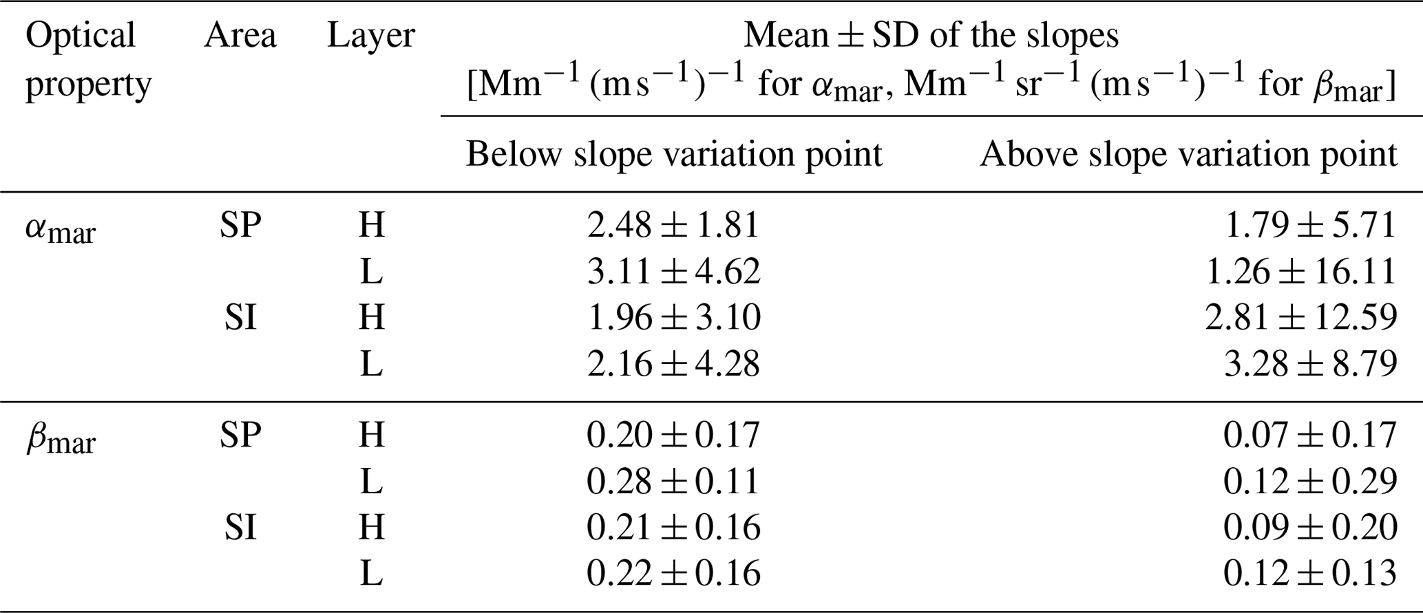
For the SP area and the SI area, the maximum wind speed can reach up to 28 m s⁻¹, while the variation in the optical properties along with wind speed is more complicated. In Fig. 9a, the α_mar values over the SP area show approximately linear growth tendencies with wind speed both at Layer_L and at Layer_H, with the exponents of the fitting functions of 0.93 and 0.82. The α_mar values increase from 72 and 52 Mm⁻¹ to 130 and 111 Mm⁻¹ for Layer_L and Layer_H, respectively. Figure 9b shows that the β_mar above the SP area increases from 2.7 and 2.1 ${\mathrm{Mm}}^{-\mathrm{1}}{\mathrm{sr}}^{-\mathrm{1}}$ to 7.0 and 5.3 ${\mathrm{Mm}}^{-\mathrm{1}}{\mathrm{sr}}^{-\mathrm{1}}$, with the exponents of the fitting functions of 0.51 and 0.38 for Layer_L and Layer_H. From Fig. 10a and b, it can be seen that the variations in α_mar and β_mar with wind speed in the SI area are similar to those in the SP area, except for that the exponents of the fitting functions of β_mar are larger than 1, i.e., 1.2 and 1.4 for Layer_L and Layer_H, respectively. In Layer_H of the SI area, α_mar at above 25 m s⁻¹ can reach up to 137 Mm⁻¹, much larger than that of around 110 Mm⁻¹ in the SP area. Panels (c) and (d) of Figs. 9 and 10 show the slopes of α_mar and β_mar with the wind speed above the SP area and the SI area. In these four panels, the dashed blue lines (mean values of the slopes at Layer_L) are all higher than the dashed red lines (mean values of the slopes at Layer_H), illustrating that the increments of α_mar and β_mar per unit of wind speed at Layer_L are larger than those at Layer_H, which implies that the input of marine aerosol driven by wind at Layer_L is stronger than at Layer_H. Focusing on Figs. 9c and 10c, it can be seen that, for both layers of the SP area and the SI area, the slopes of α_mar below 15 m s⁻¹ are almost all larger than 0, fluctuating slightly around the mean values, while the slopes of α_mar above 15 m s⁻¹ fluctuate drastically. This phenomenon may indicate that below 15 m s⁻¹, both layers continuously receive the input of marine aerosol driven by wind, but nevertheless, when the wind speed is higher than 15 m s⁻¹, the dependence of marine aerosol on wind becomes lower. As for the slopes of β_mar above the SP area and the SI area, from Figs. 9d and 10d, it is obvious that for both layers, the slopes of β_mar decrease above around 10 m s⁻¹. The corresponding variations in β_mar above the SP area and the SI area are shown in Figs. 9b and 10b, of which the β_mar values increase with higher slopes at the wind speed range of 0–10 m s⁻¹, while the slopes of increase become lower when the wind speed is above 10 m s⁻¹. This phenomenon might indicate that the increase in β_mar with wind speed includes two separate trends regarding 10 m s⁻¹ as the change point, consistent with the hypothesis raised in the analysis of the NP area. We name these two wind speeds (15 m s⁻¹ for α_mar and 10 m s⁻¹ for β_mar) “slope variation points” in this paper. Table 2 presents the averaged slopes (mean) and the corresponding standard deviations of α_mar and β_mar, below and above the slope variation points, for the two layers of the SP and SI areas. All the averaged slopes below the slope variation points are larger than those above the slope variation points, except for the α_mar in the SI area. The reason for the inverse results of α_mar in the SI area may be due to its rapid increase above 24 m s⁻¹. All standard deviations of β_mar above the slope variation points are greater than those below, indicating a more fluctuating growth phase above the slope variation points. These results could provide evidence for the statement that the wind-driven enhancement of marine aerosol includes two phases: a rapid-growth phase with high wind dependence and a slower-growth phase with higher fluctuations.

Table 2 Mean ± SD of the slopes below and above the slope variation point, grouped by area and layer.

Consequently, for all measurement cases, the marine aerosol optical properties at Layer_L are larger than those at Layer_H in any identical wind speed interval, indicating that the MABL may receive more marine aerosol produced and transported from the sea–air interface, while the higher layer above the MABL with the upper boundary of 2 km can also be affected by the marine aerosol, but to a lesser extent. The mean slope values of α_mar and β_mar at Layer_L are all larger than at Layer_H, which implies that the marine aerosol enhancements caused by the background wind are more intense at the MABL. It should be noted that the slopes change as α_mar and β_mar increase with wind speed. The slope variation point of α_mar (15 m s⁻¹) is greater than that of β_mar (10 m s⁻¹), and above it the enhancement rate becomes lower. This could illustrate that the impact of wind on marine aerosol enhancement includes two phases, one of which is a rapid-growth phase with a high dependence on wind and the other is a slower-growth phase with more fluctuations after the slope variation points.

4.4 Dependency of aerosol optical depth and lidar ratio on wind speed

4.4.1 Marine aerosol optical depth versus wind speed

As introduced in Sect. 1, almost all the previous studies on the relationship between marine aerosol optical properties and wind speed have focused on the AOD of marine aerosol. In this study, an attempt on the averaged 0–2 km AOD_mar of individual wind speed grid calculation has also been conducted to compare the AOD_mar–wind speed relationship from a previous study (Kiliyanpilakkil and Meskhidze, 2011). The AOD_mar of each single profile is acquired by integrating Aeolus-retrieved α_mar within 2 km. The wind speed profiles are also averaged over 2 km to match the AOD_mar data. Then the relationship between the AOD_mar and the wind speeds is obtained by averaging the AOD_mar in each wind speed interval (0–30 m s⁻¹, stepped by 1 m s⁻¹). The AOD_mar–wind speed relationship is also investigated using the products from the A-Train satellites (Kiliyanpilakkil and Meskhidze, 2011). “Clean marine” aerosol AOD at 532 nm above the ocean surface (up to 2 km) provided by CALIOP, and 10 m daily wind speed provided by AMSR-E, were used. It should be noted that the wind speed used in Kiliyanpilakkil and Meskhidze (2011) is the daily ocean surface wind speed, different from that used in this study, which is the instantaneous layer-averaged wind speed. Collecting the data for the period from 2006 to 2011 over 15 remote ocean regions worldwide, the regression curve is acquired with the averaged AOD_mar at 532 nm for each wind speed grid and the surface wind speed, which is up to 29 m s⁻¹, and the regression function is expressed as shown in Eq. (3):

$$\begin{array}{}\text{(3)}& {\text{AOD}}_{\text{mar,532}}={\displaystyle \frac{\mathrm{0.15}}{\mathrm{1}+\mathrm{6.7}\cdot e^{-\mathrm{0.17}\cdot U_{\mathrm{10}}}}},\end{array}$$

where U₁₀ represents the daily 10 m ocean surface wind speed.

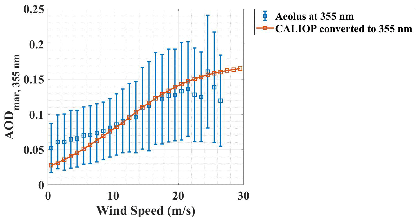
Figure 11 AOD_mar at 355 nm versus wind speed. The blue squares and the corresponding error bars represent the AOD_mar means and standard deviations along the wind speed grid of all three study areas in this study. The red squares and line represent AOD_mar at 355 nm along the wind speed grid converted from the regressive relationship between AOD_mar at 532 nm and the ocean surface wind speed reported by Kiliyanpilakkil and Meskhidze (2011).

As described above, the AOD_mar 'data source (from spaceborne lidar observations), the study areas (remote ocean regions globally), and the wind speed range (0–29 m s⁻¹) of the AOD_mar–wind speed relationship exploration in Kiliyanpilakkil and Meskhidze (2011) match well with those of this study. Hence, we select the AOD_mar–wind speed relationship established by Kiliyanpilakkil and Meskhidze (2011) for comparison. Additionally, due to the different wavelengths of AOD_mar used in this study (355 nm) and in Kiliyanpilakkil and Meskhidze (2011) (532 nm), the conversion of the AOD_mar at 532 nm to the AOD_mar at 355 nm is performed by applying the typical Ångström exponent of marine aerosol. It is reported that the Ångström exponent of marine aerosol is related to the surface wind speed, and a linear relationship has been established as given in Eq. (4) (Sayer et al., 2012):

$$\begin{array}{}\text{(4)}& A\left(\text{ws}\right)=\mathrm{0.69}-\mathrm{0.030}\cdot \text{ws},\end{array}$$

where A represents the Ångström exponent and ws represents the wind speed. Then the AOD_mar at 532 nm can be converted to the AOD_mar at 355 nm by Eq. (5):

$$\begin{array}{}\text{(5)}& \begin{array}{rl}{\displaystyle }{\text{AOD}}_{\text{mar,355\hspace{0.17em}nm}}\left(\text{ws}\right)& {\displaystyle }=\exp \left[A\left(\text{ws}\right)\cdot \ln {\displaystyle \frac{\mathrm{532}}{\mathrm{355}}}\right]\\ {\displaystyle }& {\displaystyle }\cdot {\text{AOD}}_{\text{mar,532\hspace{0.17em}nm}}\left(\text{ws}\right).\end{array}\end{array}$$

In Fig. 11, the averaged AOD_mar and corresponding standard deviations at 355 nm of all three study areas along the wind speed grid are represented by the blue squares and error bars, while the regression curve of AOD_mar at 355 nm versus wind speed converted from Eq. (3) is represented by the red squares and line. Although instantaneous layer-averaged wind speed and the daily ocean surface wind speed are used in this study and in Kiliyanpilakkil and Meskhidze (2011) individually, a similar trend of AOD_mar at 355 nm versus wind speed is obtained. It can be seen that AOD_mar increases with wind speed, and the slope of AOD_mar becomes higher along the wind speeds when the wind speed is below 15 m s⁻¹, while the variation in AOD_mar becomes slower above 15 m s⁻¹. The converted CALIOP AOD_mar values are lower than the Aeolus-retrieved AOD_mar values at 0–10 m s⁻¹. Nevertheless, the former are all in the standard deviation range of the latter, and thus the Aeolus-retrieved AOD_mar values and their variation along the wind speed are considered reasonable. The lower AOD_mar from CALIOP after wavelength conversion at low wind speed may arise from using a fixed LR_mar of 20 sr at 532 nm for CALIOP AOD_mar retrievals, while LR_mar can vary with a quite large range of 10–90 sr (Masonis et al., 2003). The possible uncertainties in the CALIOP-retrieved AOD_mar at 532 nm are discussed in detail in Kiliyanpilakkil and Meskhidze (2011). Furthermore, as discussed in Sect. 4.4.2 of this paper, the particle size of marine aerosol and LR_mar will vary with wind speed, so using the CALIOP AOD_mar retrieved with the fixed LR_mar may introduce additional error in exploring the relationship between AOD_mar and wind speed. Therefore, the use of Aeolus-retrieved AOD_mar, which is integrated by an independently retrieved extinction coefficient without the assumption of LR_mar, could make the AOD_mar–wind speed relationship more reliable.

4.4.2 Marine aerosol lidar ratio versus wind speed

As one of the intensive optical properties, LR_mar is independent of aerosol concentration. It is reported that LR_mar depends on particle size, and specifically, with the reduction in the coarse mode, the total LR turns out to increase (Masonis et al., 2003). The possible reason for this phenomenon is that as the particles become smaller, the extinction is enhanced by the increasing sideward scattering and the backscatter gets weaker due to the decrease in the scattering cross section (Haarig et al., 2017). The Aeolus Level-2A product provides the particle extinction-to-backscatter ratio calculated with the raw β, which lacks the depolarized part, as mentioned in Sect. 3. In this work, the corrected LR_mar is acquired by dividing the marine aerosol extinction by the marine aerosol depolarization-corrected backscatter. The calculation of the averaged LR_mar along wind speed grids has been performed by averaging the LR_mar values of each 1 m s⁻¹ wind speed bin, and the standard deviations are acquired as well. It should be noted that before the statistical calculations are carried out, the outliers are eliminated by the boxplot analysis method presented in Sect. 3.

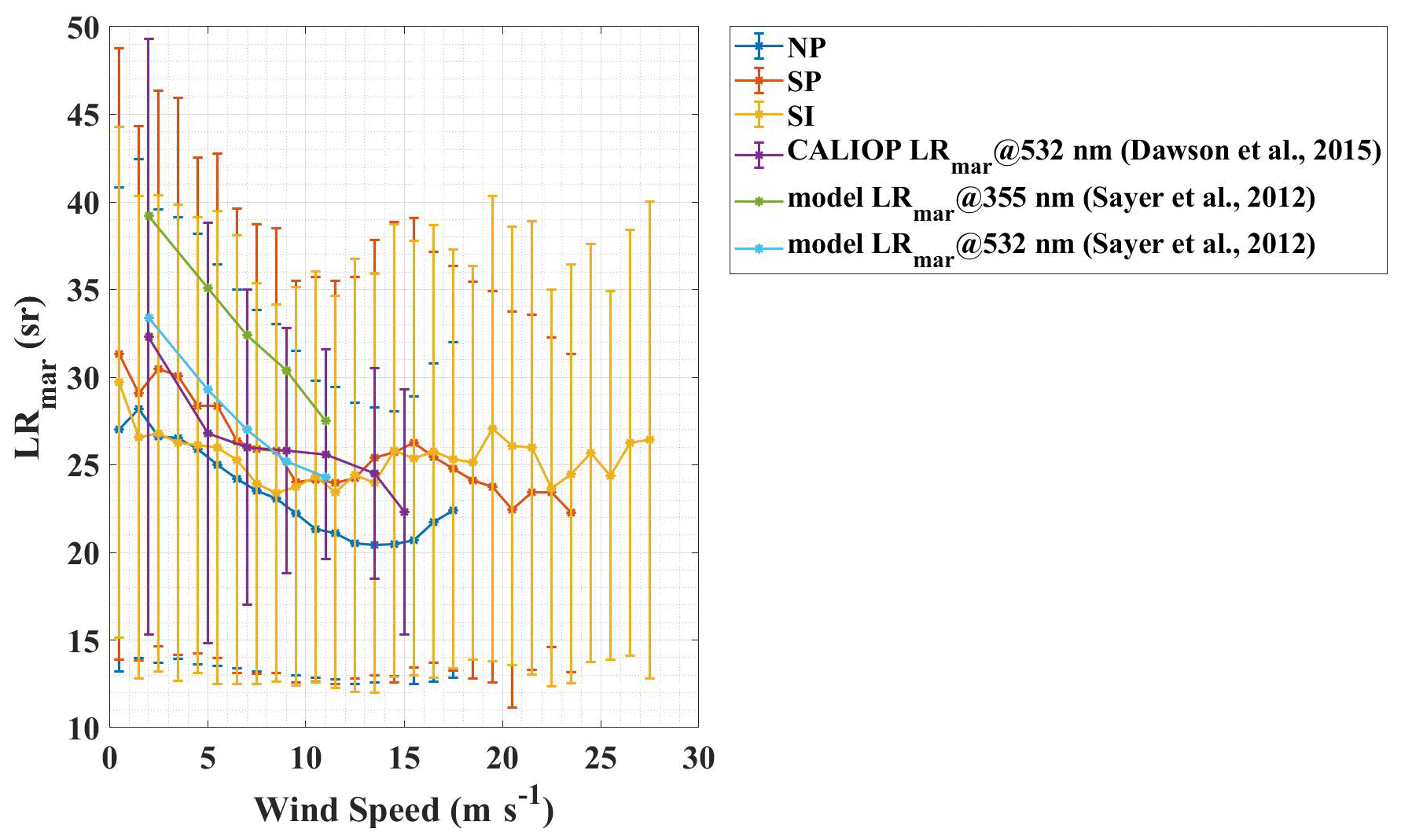
Figure 12 LR_mar versus wind speed. The dark blue curve, red curve, yellow curve, and the corresponding error bars represent the averaged LR_mar values and their standard deviations above the NP area, the SP area, and the SI area, respectively. The purple curve and the corresponding error bars represent the CALIOP-retrieved LR_mar at 532 nm (Dawson et al., 2015). The green curve and the light blue curve represent the modeled LR_mar at 355 and at 532 nm, respectively (Sayer et al., 2012).

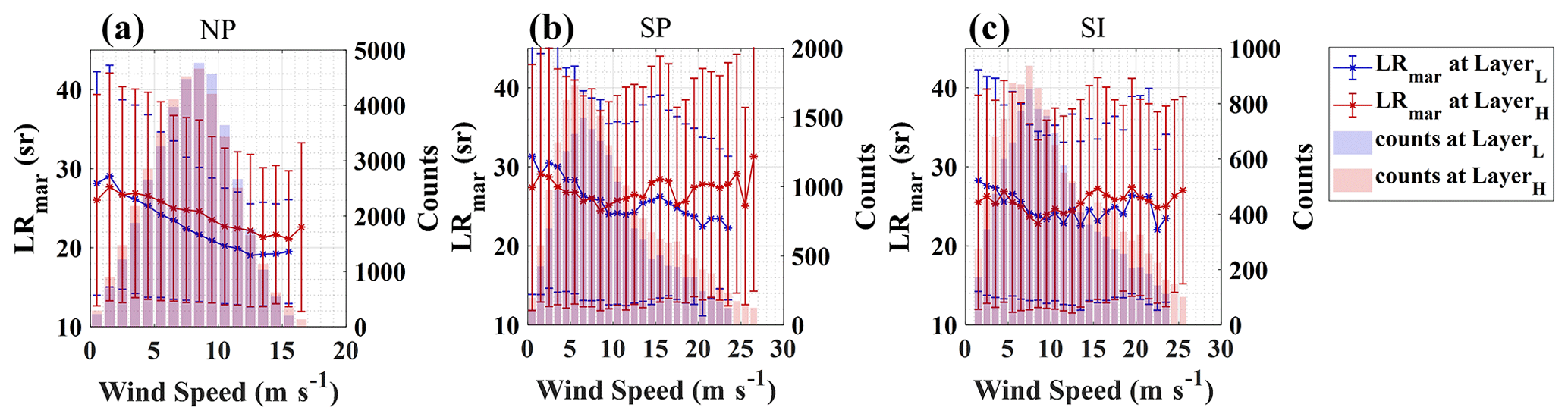
Figure 13 Averaged LR_mar versus wind speed, at Layer_L and Layer_H, in (a) the NP area, (b) the SP area and (c) the SI area, respectively.

In Fig. 12, 0–2 km averaged LR_mar variations along with the wind speed above the NP area, the SP area, and the SI area are represented as blue, red, and yellow curves, respectively. Generally, the clear downward trend of the LR_mar at relatively low wind speeds (0–14 m s⁻¹ of the NP area, 0–9 m s⁻¹ of the SP area, and 0–10 m s⁻¹ of the SI area) can be observed in all cases. The results reported in this paper are similar to those of previous studies, of which Dawson et al. (2015) and Sayer et al. (2012) investigated the relationship between LR_mar and wind speed utilizing measured LR_mar and modeled LR_mar, respectively. Combining the corrected CALIOP-retrieved LR_mar at 532 nm and 10 m ocean surface wind speed from AMSR-E, the negative correlation between LR_mar and wind speed is acquired with the wind speed bins from 0 m s⁻¹ up to > 15 m s⁻¹, shown as the purple curve in Fig. 12 (Dawson et al., 2015). The modeled LR_mar at 355 and at 532 nm also presents decreasing trends with the wind speed increases, presented as the green curve and the light blue curve in Fig. 12 (Sayer et al., 2012). These results seem to imply that the particle size of marine aerosol becomes larger as the wind speed increases for a low wind speed range. This phenomenon is explained by the shift in the volume size distribution of marine aerosol with wind speed: as wind speed increases, the fine mode volume size distribution of marine aerosol declines, while the coarse mode distribution becomes larger (Dawson et al., 2015; Smirnov et al., 2003; Sayer et al., 2012). The CALIOP LR_mar and the modeled LR_mar are all larger than the LR_mar of this study but are all in the standard deviation ranges. According to Groß et al. (2011, 2015), Bohlmann et al. (2018), and Floutsi et al. (2023), the pure LR_mar at 355 nm can vary from 10 to 40 sr, with an average of around 20 sr, and thus the averaged LR_mar values in this study are considered reasonable. In the medium wind speed range (14–18 m s⁻¹ of the NP area, 9–16 m s⁻¹ of the SP area, and 10–20 m s⁻¹ of the SI area), the LR_mar values show upward trends, implying that the marine aerosol particles might be broken down into smaller ones as the wind speed increases. At the very high wind speeds above the SP area (> 16 m s⁻¹) and the SI area (> 20 m s⁻¹), LR_mar again decreases with wind speed, which indicates that the particle size of marine aerosol becomes larger at these wind speed conditions.

Figure 13 shows the LR_mar variations at Layer_L and Layer_H along the wind speed grid in three study areas. Some divergences in the LR_mar variations between the layers can be detected. As for the NP area, the variation in LR_mar at Layer_L is from 29 sr at 1–2 m s⁻¹ to 19 sr at 12–13 m s⁻¹, larger than that at Layer_H which is from 28 sr at 1–2 m s⁻¹ to 21 sr at 15–16 m s⁻¹. Regarding the SP area and the SI area, the downward trend of LR_mar in the high wind speed condition as mentioned above is not apparent at Layer_H. Moreover, at Layer_H, LR_mar can reach up to 27–28 sr at 15–25 m s⁻¹, close to that at 0–5 m s⁻¹, implying that the marine aerosol particle sizes at low and high wind speeds are similar.

Generally, the LR_mar dependence on wind speed shows a downward trend at relatively low wind speed, then an upward trend at medium wind speed, and finally a downward trend again at very high wind speed (if present), which implies that the marine aerosol particle size initially increases with wind speed, then might be broken down into smaller sizes by the enhanced wind speed, and finally becomes larger again. Several differences in the LR_mar variations with wind speed appear between the three study areas and the two vertical layers, which may be due to the different meteorological and environmental conditions of the areas and layers.

5 Summary and conclusion

By utilizing particle optical property data (Level-2A products) and wind vector data (Level-2C products) provided by ALADIN onboard the Aeolus satellite, the correlations between marine aerosol optical properties at 355 nm and the instantaneous co-located wind speed over remote ocean areas were investigated at two separate vertical atmospheric layers (0–1 and 1–2 km, corresponding to the heights within and above the marine atmospheric boundary layer (MABL)), revealing the effect of wind speed on marine aerosol within and above the MABL over remote oceans.

Several data processing procedures were conducted to obtain pure marine aerosol data from Aeolus observations. First, three study areas located in remote oceans were selected. These areas were named the North Pacific (NP) area, the South Pacific (SP) area, and the South Indian (SI) area, respectively. The dominance of marine aerosol in these areas was then examined using the aerosol classification data provided by the VFM products of CALIOP. The proportions of marine aerosol in these areas are all larger than 79 %, while the percentage sums of marine aerosol and dusty marine aerosol are all above 90 %. Following quality control, cloud screening was performed using specific criteria (relative humidity and backscatter ratio). of the data, 9 %, 35 %, and 40 % were identified as cloud contaminated in the altitude range of 0–2 km and were subsequently eliminated for the NP area, the SP area, and the SI area, respectively. Finally, the backscatter correction was applied to the Aeolus Level-2A product. These procedures allowed us to obtain reliable, cloud-free marine aerosol optical properties and the corresponding wind speeds.

The correlations between the marine aerosol extinction coefficient (α_mar) and backscatter coefficient (β_mar) at 355 nm, as well as the wind speed, were analyzed at two separate layers for the three study areas, respectively. It was found that the Aeolus observations can provide evidence of the fact that both the layers within and above the MABL receive marine aerosol input produced and transported from the sea–air interface. Moreover, the marine aerosol load in the MABL is stronger than that at the higher layer. The enhancement of α_mar and β_mar caused by wind is more intense at the MABL. This may be due to the proximity of the MABL to the sea–air interface, making it more susceptible to such effects. Furthermore, the slope variation points (15 m s⁻¹ for α_mar and 10 m s⁻¹ for β_mar) were found during α_mar and β_mar to increase with the wind speed. Above these slope variation points, the growth rates become lower. This phenomenon implies that the wind-driven enhancement of marine aerosol includes two phases, one of which is a rapid-growth phase with a high dependence on wind and the other is a slower-growth phase with higher fluctuations after the slope variation points. The α_mar–wind speed curves and the β_mar–wind speed curves were fitted by power-law functions and the corresponding R² were all higher than 0.9 for both layers and for all study areas. In addition, the relationship between AOD_mar at 355 nm and wind speed shows a quite consistent tendency with the regression function found in a previous study (Kiliyanpilakkil and Meskhidze, 2011) that compared CALIOP-retrieved AOD_mar and 10 m surface wind speed. The marine aerosol lidar ratio (LR_mar) and its particle size have a negative relationship. From the examination of the correlation between LR_mar and wind speed, it can be inferred that as the wind speed increases, the particle size of marine aerosol appears to become larger in the relatively low wind speed range, then could be broken up into smaller particles by wind at higher wind speeds, and ultimately turns out in a larger state again at very high wind speeds. As α_mar and β_mar are affected by both particle concentration and size, this reminds us that the increase in α_mar and β_mar with wind speed may not only be due to the enhancement of particulate quantity produced from the sea–air interface, but may also be impacted by the variation in size.

The regression models of α_mar–wind speed and β_mar–wind speed at two vertical layers above the three study areas are inconsistent, while the meteorological and environmental parameters, apart from the wind, differ across various regions. The production, entrainment, transport, and removal of marine aerosol above the ocean are not only dominated by the wind but also impacted by other meteorological and environmental factors, e.g., atmospheric stability, sea and air temperature, relative humidity, and others. This implies that in order to obtain more precise α_mar and β_mar models, in addition to wind speed, the abovementioned factors should be included in the establishment of the models.

This study demonstrates the ability of Aeolus to quantify interactions between aerosols and wind speeds in poorly observed ocean regions through a synergy of aerosol and wind observations based on its unique setup. The analyses of these interactions deepen our understanding of the effect of wind speed on marine aerosol optical properties over remote oceans by providing vertical information and demonstrating that their relationships are more complex than a linear or exponential relation. For the upcoming launch of EarthCARE (Earth Cloud Aerosol and Radiation Explorer) and the future planned Aeolus-2 and other vertical profile observation lidar satellites, aerosol and wind parameters with higher vertical resolution will become available. These parameters, including lidar ratios and depolarization ratios, will be helpful for the comprehension of the relationships between marine aerosol and wind speed.