Utility of Geostationary Lightning Mapper-derived lightning NO emission estimates in air quality modeling studies

Lightning is one of the primary natural sources of nitric oxide (NO), and the influence of lightning-induced NO (LNO) emission on air quality has been investigated in the past few decades. In the current study an LNO emissions model, which derives LNO emission estimates from satellite-observed lightning optical energy, is introduced. The estimated LNO emission is employed in an air quality modeling system to investigate the potential influence of LNO on tropospheric ozone. Results show that lightning produced 0.174 Tg N of nitrogen oxides (NO_x = NO + NO₂) over the contiguous US (CONUS) domain between June and September 2019, which accounts for 11.4 % of the total NO_x emission. In August 2019, LNO emission increased ozone concentration within the troposphere by an average of 1 %–2 % (or 0.3–1.5 ppbv), depending on the altitude; the enhancement is maximum at ∼ 4 km above ground level and minimum near the surface. The southeastern US has the most significant ground-level ozone increase, with up to 1 ppbv (or 2 % of the mean observed value) difference for the maximum daily 8 h average (MDA8) ozone. These numbers are near the lower bound of the uncertainty range given in previous studies. The decreasing trend in anthropogenic NO_x emissions over the past 2 decades increases the relative contribution of LNO emissions to total NO_x emissions, suggesting that the LNO production rate used in this study may need to be increased. Corrections for the sensor flash detection efficiency may also be helpful. Moreover, the episodic impact of LNO on tropospheric ozone can be considerable. Performing backward trajectory analyses revealed two main reasons for significant ozone increases: long-distance chemical transport and lightning activity in the upwind direction shortly before the event.

1 Introduction

The air quality community is concerned about nitrogen oxides (NO_x), a group of highly reactive gases – nitric oxide (NO) and nitrogen dioxide (NO₂) – with NO₂ being regulated by the US Environmental Protection Agency (USEPA) as one of the criteria air pollutants. One reason is that, in the presence of sunlight and water vapor, NO_x can react with volatile organic compounds (VOCs) to produce ozone (O₃), a secondary air pollutant that has adverse health effects on susceptible individuals (Chen et al., 2007; Post et al., 2012; Caiazzo et al., 2013; USEPA, 2015, 2021) and is harmful to the environment (Van Dingenen et al., 2009; Fuhrer et al., 2016; Dinan et al., 2021). After decades of efforts to reduce anthropogenic NO_x emissions in the US (Simon et al., 2015), the relative importance of naturally emitted NO_x to air quality is expected to increase (Kang et al., 2019a). Lightning, an electrical discharge phenomenon caused by charge separation and accumulation during a thunderstorm (Verma et al., 2021), is an important natural source of NO (Pour-Biazar and McNider, 1995). The intense heating and subsequent rapid cooling of air that occur due to a lightning discharge convert stable nitrogen (N₂) and oxygen (O₂) into NO (Bond et al., 2001). It was estimated that lightning-induced NO (LNO) emission accounts for 10 %–15 % of the global NO_x budget (Schumann and Huntrieser, 2007) and more than 80 % of the upper-tropospheric NO_x in summer (Cooper et al., 2009).

Because NO production from lightning is sensitive to various factors, such as peak current, channel length, strokes per flash, air density, and energy dissipation rate (Cooper et al., 2009; Koshak et al., 2014a, 2015; Murray, 2016), the amount of NO produced from lightning is still highly uncertain, even though considerable research efforts have been devoted to quantifying the amount of NO produced by lightning flashes, including theoretical calculations (e.g., Chameides et al., 1977), laboratory experiments (e.g., Peyrous and Lapeyre, 1982), cloud-scale chemical transport model simulations (e.g., Ott et al., 2010), ground-based observations (e.g., Wada et al., 2019), and satellite-based column measurements (e.g., Bucsela et al., 2010; Pickering et al., 2016). A comprehensive literature review by Schumann and Huntrieser (2007) reported that the best estimate of the LNO production rate is 15 × 10²⁵ molecules of NO per flash with uncertainty factors ranging from 0.13 to 2.7, which is equivalent to 250 (32.5–675) mol of NO production per flash. A subsequent review by Murray (2016) updated the uncertainty range to be 17–700 mol of NO production per flash.

With the availability of lightning flash data from the National Lightning Detection Network (NLDN) (Orville et al., 2002, 2011), a reputable ground-based lightning detection network that has a high (∼ 90 %–95 %) cloud-to-ground (CG) flash detection efficiency (DE) over the contiguous US (CONUS), various models and schemes have been developed to estimate LNO emission and investigate its impact on ozone prediction in regional chemical transport models (Kaynak et al., 2008; Smith and Mueller, 2010; Allen et al., 2012; Koshak et al., 2014a; Wang et al., 2015; Kang and Pickering, 2018; Kang et al., 2019a, b, 2020). For instance, Allen et al. (2012) introduced an LNO parameterization scheme, which utilizes monthly NLDN (mNLDN) flash data, into the Community Multiscale Air Quality (CMAQ) model (Byun and Schere, 2006; Appel et al., 2021). The mNLDN scheme assumes that total column LNO emission is proportional to model-predicted convective precipitation (CP) with local adjustment so that the monthly average CP-based flash rate in each model grid cell matches the NLDN-based monthly mean total flash rate. The total column LNO emission is then distributed vertically based on a preliminary version of the segment altitude distributions derived by Koshak et al. (2014a) using North Alabama Lightning Mapping Array (NALMA) data (Goodman et al., 2005). Kang et al. (2019a) simplified the mNLDN scheme in CMAQ by using only gridded hourly NLDN (hNLDN) flash data to ingest LNO emission into model grid cells directly. However, since the hNLDN scheme is not dependent on the model-predicted CP field, discrepancies between the time and location of the released LNO emission and convective activity, as well as other convectively transported ozone precursors, may exist. In addition, Kang et al. (2019a) also introduced a parameter scheme (pNLDN) that is based on linear and log-linear regression parameters derived from multi-year NLDN lightning flash data and the model-predicted CP field, which can be used when lightning observations are not available (such as air quality forecasts and future climate studies).

Further, satellite-based lightning observations can also be used to estimate LNO production (e.g., Bucsela et al., 2010; Pickering et al., 2016; Koshak et al., 2014b; Koshak, 2017). Koshak et al. (2014b) and Koshak (2017) proposed an approach that derives LNO emission estimates independent of model fields using satellite lightning imager flash-optical-energy data (e.g., as from the Tropical Rainfall Measuring Mission, TRMM, Lightning Imaging Sensor, LIS (Cecil et al., 2014), and geostationary lightning mappers (see below), respectively). It is referred to as the β method since it relies on computing a scalar denoted as β that converts the satellite-detected flash optical energy (typically hundreds of femtojoules as measured from geostationary platforms) to an estimate of the total lightning flash energy (typically gigajoules), and consequently to LNO. However, because TRMM–LIS is a low-Earth-orbiting satellite, it cannot record the entire life cycle of a thunderstorm (Bucsela et al., 2010). As a result, using TRMM–LIS data cannot explicitly characterize the diurnal variation in LNO emission over a specific region. This limitation can be overcome by using observations from the Geostationary Operational Environmental Satellite R-series (GOES-R) Geostationary Lightning Mapper (GLM), which has a similar instrument design and data processing algorithm to TRMM–LIS (Goodman et al., 2013; Schmit et al., 2017). GLM is the first operational lightning mapper in the geostationary orbit and continuously monitors lightning activity over the Americas and adjacent ocean regions. It collects lightning optical pulses at 777.4 nm (i.e., the center of a prominent oxygen emission triplet in the lightning spectra) with a nadir staring, high-speed charge-coupled device (CCD) array.

Our recent paper, Wu et al. (2023), introduced an offline LNO emission model that utilizes GOES-16 and GOES-17 GLM (hereinafter referred to as GLM-16 and GLM-17) lightning observations to prepare LNO emission input for regional air quality modeling systems by implementing the β method introduced in Koshak et al. (2014b) and Koshak (2017). As a follow-up study, this paper applies the GLM-estimated LNO emission in air quality model simulations to study how it would affect ozone simulation. One caveat is that the LNO emission model does not constrain the time and location of LNO production using the model cloud field. Therefore, desynchronization between model clouds and LNO emission adds uncertainty. This issue will be addressed in our future study by assimilating GOES cloud observations (White et al., 2018, 2022) to improve model cloud placement. Another way to resolve such desynchronization is to conduct lightning data assimilation (Heath et al., 2016; Kang et al., 2022a) in the upstream meteorological simulation with the same lightning flash data. The rest of this paper is organized as follows: Sect. 2 provides descriptions of the Wu et al. (2023) GLM-based LNO emission model, Sect. 3 states how air quality simulations are conducted, Sect. 4 presents simulation results and discusses the potential impact of LNO emission on ozone prediction, and Sect. 5 summarizes the key findings and lists future work.

2 GLM-based LNO emission model

2.1 Column total LNO production

The LNO emission model described in Wu et al. (2023) first estimates column total LNO production from the GLM Level 2 data product, which is currently distributed via the National Oceanic and Atmospheric Administration (NOAA) Comprehensive Large Array-data Stewardship System (CLASS) (https://www.class.noaa.gov, last access: 28 August 2022). The GLM Level 2 data product contains the time, geographic location, areal coverage, and radiant energy information of three lightning elements – event (pixel-level lightning registered by GLM over a 2 ms integration window), group (one or more simultaneous events detected in adjacent pixels), and flash (a set of sequential groups occurring within 330 ms and 16.5 km). Since the temporal resolution of the product is much higher than needed by air quality modeling systems, only flash-level data are processed to improve computational efficiency. Previous assessments (Marchand et al., 2019; Bateman and Mach, 2020; Bateman et al., 2021; Blakeslee et al., 2020; Murphy and Said, 2020; Zhang and Cummins, 2020; Rutledge et al., 2020) estimated that GLM flash-level DE is greater than 70 % on average, which varies with storm type and is generally higher at night than during the day. However, a few studies (e.g., Murphy and Said, 2020; Bateman and Mach, 2020; Blakeslee et al., 2020) pointed out that GLM flash DE is significantly depleted on the edge of the sensor field of view (e.g., over the northwestern US for GLM-16). The recent study by Wu et al. (2023) showed that significantly more (fewer) NLDN-detected CG flashes could be matched to GLM-16 flashes than GLM-17 flashes east (west) of 106.2^∘ W. Therefore, to reduce the uncertainty caused by diminished GLM flash DE, GLM-16 flashes east of 106.2^∘ W and GLM-17 flashes west of 106.2^∘ W are selected, merged, aggregated into hourly values, and gridded onto pre-defined model grid cells before subsequent calculations.

With the core assumption that the GLM-detected flash optical energy is proportional to the total flash energy (i.e., the total stored electrostatic flash energy typically measured in gigajoules and that is released as acoustical and electromagnetic energy in the discharge), the amount of NO (in moles) produced by flash k (P_k) is estimated by Koshak et al. (2014b) and Koshak (2017) as

$$\begin{array}{}\text{(1)}& P_k={\displaystyle \frac{Y}{{\mathit{\beta }}_k{N}_{\mathrm{A}}}}{Q}_k,\end{array}$$

where β_k is the fraction of the total lightning-released optical energy detected by GLM for flash k, N_A (6.022 × 10²³ molecules per mole) is Avogadro's number, Y (∼ 10¹⁷ molecules per Joule) is the thermochemical yield of NO (Borucki and Chameides, 1984), and Q_k is the GLM-detected optical energy (in Joules) from flash k (provided by GLM flash-optical-energy data). The only variable needed for obtaining the value of P_k is the dimensionless scaling factor β_k, which is sensitive to various lightning and cloud scattering properties and GLM sensor characteristics (Koshak et al., 2014b; Wu et al., 2023). To make this method feasible, it is assumed that many (but not all) of these factors average out for a large number of GLM flashes and numerous types of thundercloud structures over diverse geographical areas. Assuming that the particular β_k in Eq. (1) can be replaced by a fixed (mean) value β, then Eq. (1) can be re-written as

$$\begin{array}{}\text{(2)}& P_k={\displaystyle \frac{Y}{\mathit{\beta }{N}_{\mathrm{A}}}}{Q}_k.\end{array}$$

It is important to note that this equation provides a variable flash-to-flash estimate of LNO production (hence the k subscript in the production variable P_k). Only the value β is chosen as fixed. Now, to obtain a representative value of β, multiple years of GLM flash-optical-energy data are needed, and Eq. (2) is rewritten as

$$\begin{array}{}\text{(3)}& \mathit{\beta }={\displaystyle \frac{Y}{N_{\mathrm{A}}}}{\displaystyle \frac{{\sum }_{k=\mathrm{1}}^N{Q}_k}{{\sum }_{k=\mathrm{1}}^N{P}_k}}={\displaystyle \frac{Y}{N_{\mathrm{A}}}}{\displaystyle \frac{{\sum }_{k=\mathrm{1}}^N{Q}_k}{N\stackrel{\mathrm{‾}}{P}}},\end{array}$$

where N is the total number of GLM flashes within an extended period (over the entire observational domain), and $\stackrel{\mathrm{‾}}{P}$ is the average amount of NO produced by lightning flashes. In recent air quality modeling studies, 250 to 500 mol per flash is typically used for $\stackrel{\mathrm{‾}}{P}$ (Allen et al., 2010; Ott et al., 2010; Koshak et al., 2014b; Koshak, 2017; Wang et al., 2015; Zhu et al., 2019; Kang et al., 2019a, b, 2020). For this study, the LNO emission model assumes that a lightning flash would produce 250 mol of NO on average, a commonly cited LNO production rate in the literature (Schumann and Huntrieser, 2007). Processing almost 3 years (February 2019–December 2021) of GLM data within the CONUS yields an estimate of 1.5336 × 10⁻²² for β. Once β is known, NO production by each lightning flash is estimated using Eq. (2), and total column LNO emission can be determined.

The derivation of the column total LNO production has several sources of uncertainty. First, the fixed value of β varies linearly with the assumed globally averaged LNO production rate ($\stackrel{\mathrm{‾}}{P}$); i.e., this method constrains the geographic distribution of LNO emission but not its globally averaged magnitude. The value $\stackrel{\mathrm{‾}}{P}=\mathrm{250}$ mol per flash globally, which is currently used by the GLM-based LNO emission model as a constraint, is highly uncertain (Schumann and Huntrieser, 2007; Murray, 2016). Many factors can affect the value of $\stackrel{\mathrm{‾}}{P}$. For example, NO production is sensitive to various lightning characteristics, such as peak current, channel length, strokes per flash, air density, and energy dissipation rate (Cooper et al., 2009; Koshak et al., 2014a, 2015; Murray, 2016). A lightning discharge with a longer channel length or a higher peak current produces more NO. In the latter case, a higher peak current normally implies more area under the stroke current waveform i(t) and therefore more net energy in the discharge, and this is explicitly true for the return stroke current models for i(t). Many studies have shown that one CG flash might produce up to 10 times more NO than an intra-cloud (IC) flash (Koshak et al., 2014a; Carey et al., 2016; Lapierre et al., 2020) as CG flashes typically have stronger peak currents and longer channel lengths as well as more channel at lower altitude, where the thermochemical yield is larger, and they extend to a larger area than IC flashes (Rakov and Uman, 2003; Koshak et al., 2009, 2014a; Koshak, 2010; Mecikalski and Carey, 2018). Therefore, even though the β method utilizes flash-specific GLM-observed flash optical energy to compute LNO production on a per flash basis nicely, the value of $\stackrel{\mathrm{‾}}{P}$ is still assumed/biased, meaning it will introduce uncertainty to the LNO emission estimates. Second, not all lightning flashes are detected by GLM. Recent studies indicated that GLM flash DE is correlated with the type, geometric size, optical energy, duration of the flash, cloud optical depth, seasons, time of day, and sensor viewing geometry (e.g., Blakeslee et al., 2020; Murphy and Said, 2020; Rutledge et al., 2020; Zhang and Cummins, 2020). For example, less energetic and shorter IC flashes are less likely to be detected than CG flashes. GLM flash DE is found to be relatively lower over the Great Plains (Allen et al., 2021; Wu et al., 2023), which is possibly due to anomalous polarity storms being more common in this region and thus having more low-altitude and/or short-duration flashes (Zhang and Cummins, 2020). As a result, NO production from any missed flashes would not be counted. Third, since β is an average based on multi-year GLM flash-optical-energy data, it can be further refined as more GLM data become available. Despite all of the factors mentioned in this paragraph, an advantage of the β method is that all these uncertainties are accounted for by a single scalar (β), allowing potential improvements in future studies.

2.2 Vertical distribution of LNO emission

Generally, air quality modeling systems require three-dimensional gridded emissions as input. Since GLM lightning observations are only two-dimensional, extra information is needed to distribute the derived column total LNO emission vertically. This is accomplished by adapting monthly LNO production profiles created by the Lightning Nitrogen Oxides Model (LNOM) (Koshak, 2010; Koshak et al., 2009, 2014a) and using the climatological IC/CG ratios from Boccippio et al. (2001). It should be noted however that the IC-to-CG ratio is only used for the vertical distribution of the estimated column LNO by the GLM-based emissions model and does not adjust the emissions. The LNOM is a flash-based model that fuses laboratory results (Wang et al., 1998), theoretical results (Cooray et al., 2009), and additional simplifying assumptions discussed in Koshak et al. (2014a) with Lightning Mapping Array (LMA) (Goodman et al., 2005) and NLDN lightning observations. The LNO emission model vertically distributes LNO emission using pre-generated monthly LNOM profiles for CG and IC flashes archived at the National Aeronautics and Space Administration (NASA) Global Hydrology Resource Center (GHRC) (https://ghrc.nsstc.nasa.gov/uso/ds_docs/lnom/lnom_dataset.html, last access: 4 August 2022). To account for the different contributions of CG and IC flashes to the overall vertical profile, the climatological geographic distribution of daily IC-to-CG ratio (denoted by the Z ratio) developed by Boccippio et al. (2001) with updates from Medici et al. (2017) is applied in conjunction with the LNOM profiles to vertically distribute the total column LNO estimates. Readers are referred to Wu et al. (2023) for more details on how the LNOM profiles and the IC-to-CG ratio were applied when distributing LNO emission in the vertical direction. As demonstrated in Fig. S1 in the Supplement, the LNO emission model produces monthly LNO emission profiles with a backward C shape, which is consistent with the LNOM profiles (Koshak et al., 2014a; Wu et al., 2023). Note that using the archived LNOM profiles and the climatological IC-to-CG ratio introduces another layer of uncertainty to the derived three-dimensional LNO emission. The LNOM profiles were constructed around the NALMA and therefore are more representative of northern Alabama than other regions of the CONUS. Meanwhile, the Z ratio map was generated using multi-year satellite and ground-based lightning observations, but lightning activity varies appreciably from year to year.

3 WRF–SMOKE–CMAQ model configuration

Air quality simulations were conducted by the modeling system containing the Weather Research and Forecasting (WRF) (Skamarock et al., 2021), the Sparse Matrix Operator Kernel Emissions (SMOKE) (https://www.cmascenter.org/smoke, last access: 31 August 2022), and the CMAQ (Byun and Schere, 2006; Appel et al., 2021). The simulation period covers the months of June to September 2019, with a 10 d spin-up period in May. Model configurations were similar to our 2016 air quality modeling study (Cheng et al., 2022), with some necessary adjustments for tropospheric dynamics options based on our sensitivity tests for the 2019 study period. Readers are referred to Tables S1 and S2 in the Supplement for model configurations used in Cheng et al. (2022) as opposed to those of this study.

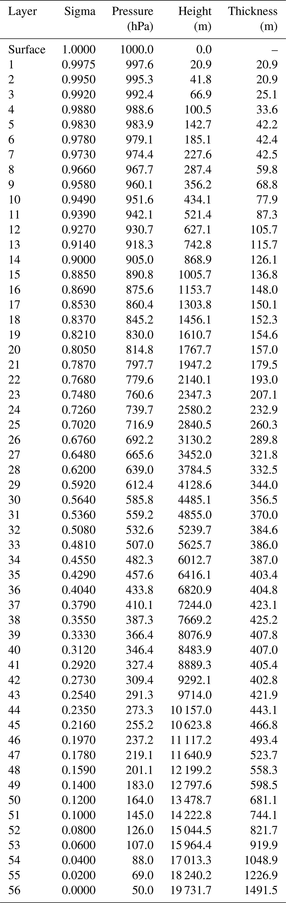
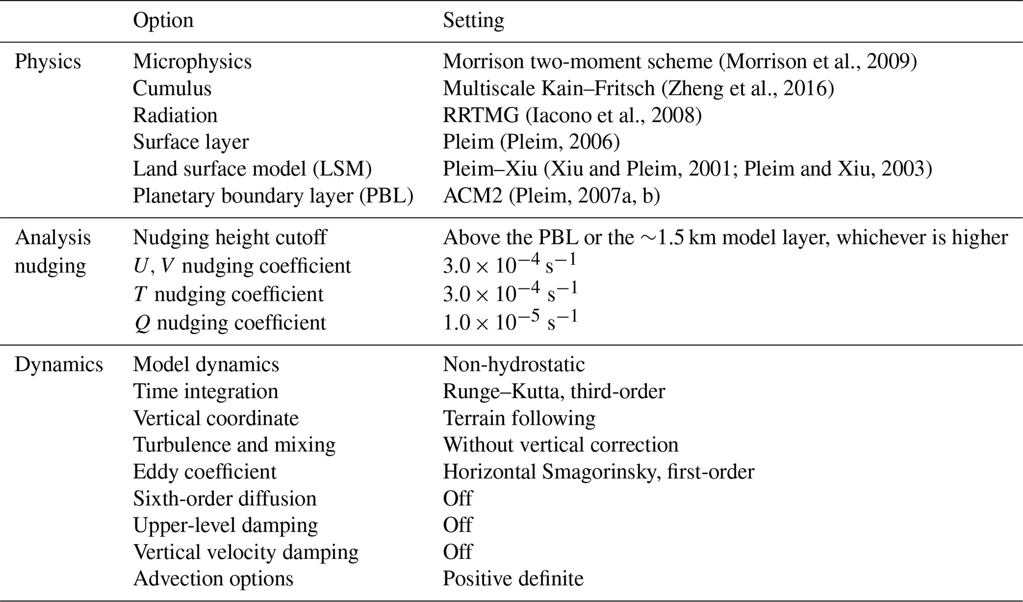
WRF version 4.3.1 (https://github.com/wrf-model/WRF/releases/v4.3.1, last access: 31 August 2022) was used to provide meteorological inputs on a 12 km domain with 471 × 311 grid cells covering the CONUS (Fig. 1). The atmosphere was divided into 56 vertical layers with varying thicknesses extending from the surface to 50 hPa, wherein 18 model layers are arranged below 1.5 km, and the lowest (surface) layer has an approximately 10 m midpoint (Table 1). WRF simulations were broken into overlapping 5.5 d run segments: the first 12 h of each run segment was discarded because it was primarily for initializing model fields; the remaining 5 d was used as input for emission processing and air quality simulations. This was done to reduce the meteorological drift while keeping the air quality simulation continuous. WRF initial and lateral boundary conditions were prepared using the North American Mesoscale Forecast System (NAM) analysis and 3-hourly forecast (https://www.ncei.noaa.gov/products/weather-climate-models/north-american-mesoscale, last access: 31 August 2022). The main physics, analysis nudging, and dynamics options used in the WRF simulation are summarized in Table 2. Note that the analysis nudging was only performed above the planetary boundary layer (PBL) height (or ∼ 1.5 km, whichever is higher) to preserve the nocturnal low-level jet (LLJ), a crucial PBL phenomenon for long-range transport of air pollutants at night (Odman et al., 2019). Also, upper-level and vertical velocity damping were turned off to minimize the impact of numerical filters on stratospheric ozone intrusion. Previous studies have suggested that stratospheric ozone intrusion accounts for approximately 10 % of the tropospheric ozone budget (Fusco and Logan, 2003; Liang et al., 2009; Kuang et al., 2012).

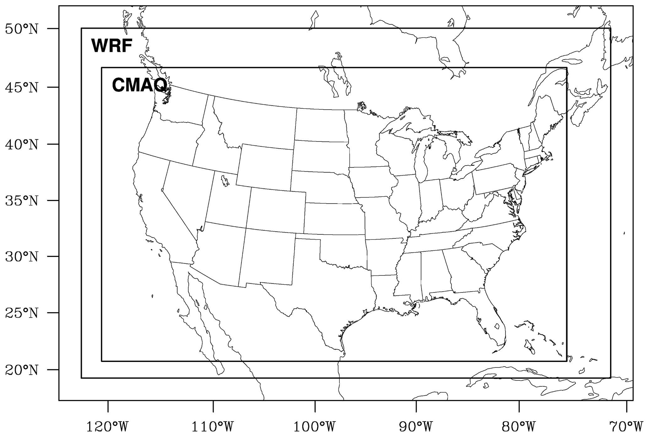
Figure 1 WRF and CMAQ model domain.

Table 1 Model vertical layers and their approximate geopotential height.

Table 2 WRF physics, analysis nudging, and dynamics options.

SMOKE version 4.7 (https://github.com/CEMPD/SMOKE/releases/SMOKEv47_Oct2019, last access: 6 September 2022) was used to prepare gridded, speciated, hourly anthropogenic emissions for subsequent CMAQ simulations. Because the collaborative 2019 emission modeling platform (EMP) (https://www.epa.gov/air-emissions-modeling/2019-emissions-modeling-platform, last access: 6 September 2022) was under development at the beginning of this study, the 2016v1 EMP (https://www.epa.gov/air-emissions-modeling/2016v1-platform, last access: 6 September 2022) was used as the base-year inventory and projected to 2019. Note that no growth factor was set for this future-year emission processing. More accurate anthropogenic emissions are expected after the release of the 2019 EMP. Point source emissions were processed in in-line modes. Biogenic emissions were generated in-line in CMAQ using BEIS version 3.6.1 (Bash et al., 2016).

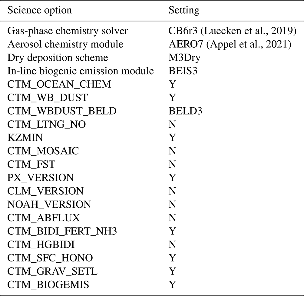
CMAQ version 5.3.3 (https://github.com/USEPA/CMAQ/releases/CMAQv5.3.3_17Aug2021, last access: 6 September 2022) was used to perform two air quality simulations on the USEPA 12US2 grid, a 12 km horizontal grid spacing with 396 × 246 grid cells covering the CONUS (Fig. 1). One is the control simulation (labeled as CNTRL), which was configured with the third revision of the Carbon Bond version 6 (CB6r3) chemical mechanism (Luecken et al., 2019) and the AERO7 aerosol module (Appel et al., 2021). Other science options are listed in Table 3. Note that none of the three CMAQ in-line LNO emission schemes (mNLDN, hNLDN, and pNLDN) was applied in the CNTRL simulation. The other is the lightning simulation (labeled as LGTNO), which added the GLM-based three-dimensional LNO emission on top of the CNTRL. Chemical initial and boundary condition input files were extracted and speciated from the Community Atmosphere Model with Chemistry (CAM-chem; Buchholz et al., 2019; Emmons et al., 2020) outputs (https://www.acom.ucar.edu/cam-chem/cam-chem.shtml, last access: 6 September 2022).

Table 3 CMAQ science options.

4 Results and discussions

4.1 Contribution of LNO to total NO_x emissions

The amount of NO_x emission from lightning, anthropogenic, and soil sources over the entire model domain was first quantified, including grid cells over Mexico, Canada, and ocean areas. As shown in Table 4, lightning flashes produced about 12.43 × 10⁹ mol NO (or equivalently 0.174 Tg N, 1 Tg = 10¹² g) from June through September 2019. The percentage contribution of LNO to total NO_x emissions is 12 %–13 % in the summer months (i.e., June, July, and August), 8 % in September, and an average of 11.4 % during the study period. These numbers are within the uncertainty range given in previous studies (Bond et al., 2001; Zhang et al., 2003; Schumann and Huntrieser, 2007; Murray, 2016; Kang and Pickering, 2018; Kang et al., 2019a) but are closer to the lower end of the range. For instance, using 5 years (1995–1999) of NLDN data, Bond et al. (2001) estimated that lightning activity produced approximately 0.323 Tg N over the CONUS in the 4-month period from June to September, which is nearly 2 times the number estimated in this study (0.174 Tg N). This difference can be attributed to the LNO production rate assumption: Bond et al. (2001) used an average production rate of ∼ 400 mol per flash (6.7 × 10²⁶ and 6.7 × 10²⁵ NO molecules per CG and IC flash, respectively; 29 % of flashes are CG), but an average production rate $\stackrel{\mathrm{‾}}{P}$ of 250 mol NO per flash was assumed in this study. Despite the difference in the amount of LNO emission, the contribution of the lightning source to the NO_x budget obtained in this study is consistent with what was indicated by Bond et al. (2001). Their results showed that lightning accounts for 11 %–14 % of total NO_x emissions in the summer months and 5 % in September, similar to the percentages summarized in Table 4. However, considering the decreasing trend of anthropogenic NO_x emissions across the CONUS in the past 2 decades, the contribution of LNO emission should be larger during the study period than given in Bond et al. (2001). In fact, recent estimates by Kang and Pickering (2018) confirmed a higher LNO contribution to total NO_x emissions, with about 20 % for the summer months of 2011 and 10 % for September 2011. This suggests that LNO emission could be underestimated in this study or overestimated in their study.

Table 4 Total monthly LNO, anthropogenic NO_x, and soil NO emissions of the model domain.

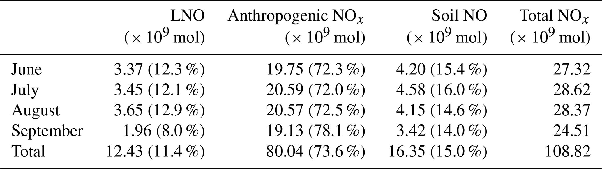
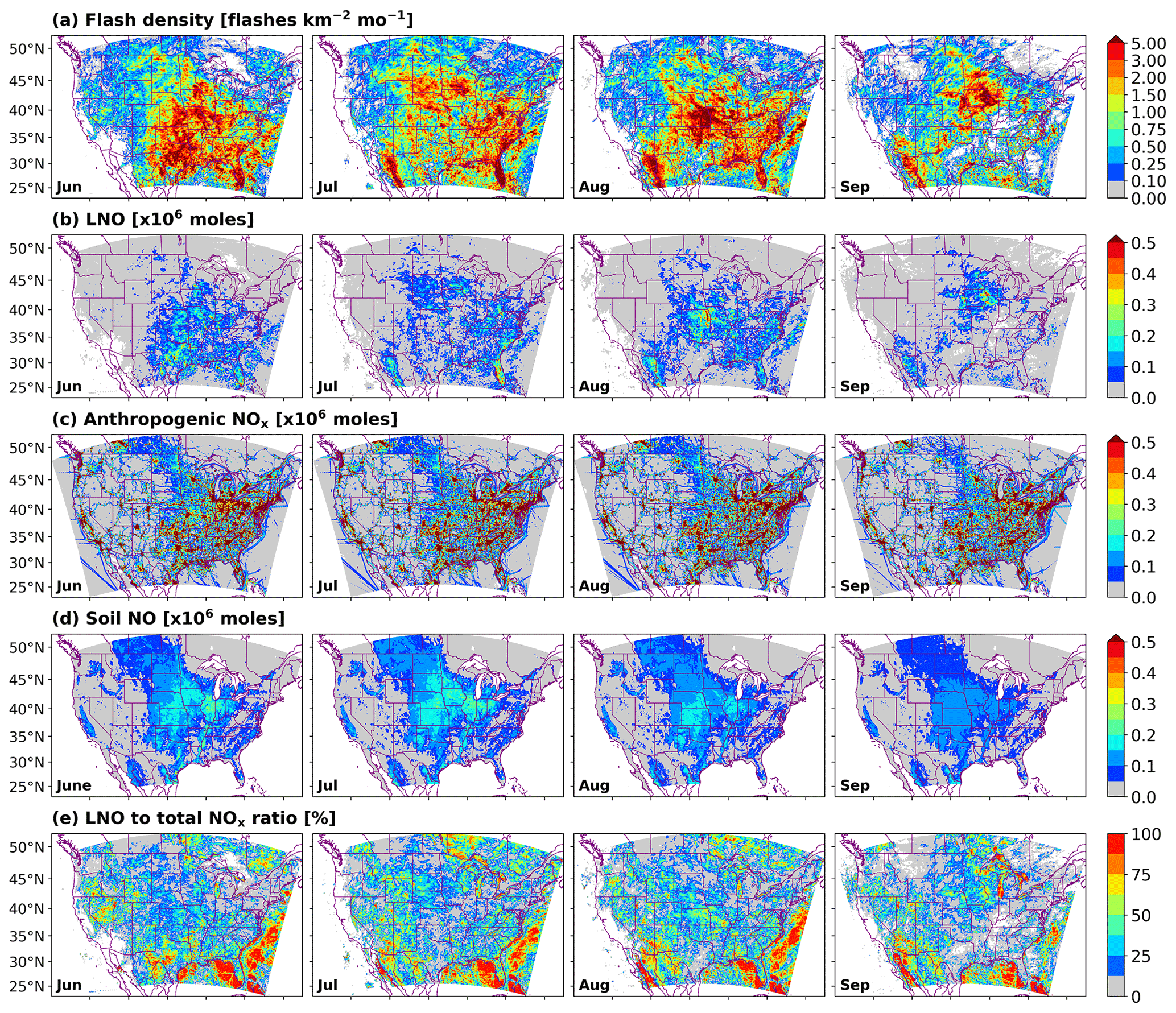
Figure 2 Spatial distribution of monthly flash density and NO_x emissions from lightning, anthropogenic, and soil sources for June through September 2019. (a) Total flashes per square kilometer per month; monthly total NO_x emissions (in millions of moles) from (b) lightning, (c) anthropogenic, and (d) soil sources per model grid cell (12 km × 12 km, or 144 km²); (e) the ratio of LNO to total NO_x emissions.

The spatial distribution of monthly flash density derived from GLM data is presented in Fig. 2. In the summer months, consistently high flash density was observed in the southeastern US, especially in Florida, along the Gulf Coast, and the East Coast. A significant number of lightning strikes also occurred in other regions, including the southern, central, and midwestern US and northwestern Mexico (to the south of Arizona and New Mexico), where the temporal variability in lightning activity was much higher. In September, the frequency of lightning decreased dramatically in the southeastern US, while Iowa and adjacent states experienced a large number of lightning events. Similar spatial patterns of flash density were presented in a previous long-term lightning climatology study by Holle et al. (2016). Note that they reported lower flash density values than in this study. This is because Holle et al. (2016) only used CG flashes to compute monthly flash density, while GLM observed both CG and IC flashes.

Figure 2 also presents the spatial distribution of monthly total NO_x emissions from lightning, anthropogenic, and soil sources. Similar to flash density, the amount of NO emitted from the lightning source varies significantly with time and location. LNO emission is generally greater in the southeastern, southern, central, and midwestern US and northwestern Mexico. Monthly LNO emission in these regions can reach 0.5 × 10⁶ mol per model grid cell (12 km × 12 km) or higher. However, this is lower than those reported by several recent studies, including Kang and Pickering (2018) and Kang et al. (2019a, b, 2020), which used a greater LNO production rate (350 mol per flash) compared to the mean value used in this study (i.e., $\stackrel{\mathrm{‾}}{P}=\mathrm{250}$ mol per flash). On the other hand, the magnitude and the spatial distribution of anthropogenic and soil NO emissions are consistent with our 2016 air quality modeling study (Cheng et al., 2022) and Kang and Pickering (2018). In addition, the contribution of lightning to total NO_x emissions is more significant in the western US and over the water, where anthropogenic NO_x emission is limited.

4.2 Impact of LNO emission on ground-level ozone and NO_x concentrations

To demonstrate the impact of LNO emission on ground-level air quality, mean differences in ground-level ozone, NO_x, and NO_y mixing ratios between two model runs were compared for the entire simulation period (Fig. 3). Ground-level ozone increase was about 0.5 ppbv (1.5 %) in the southeastern US, where lightning activity is intense (Fig. 2a). However, the most significant ground-level ozone enhancement (∼ 1.0 ppbv or 3 %) was captured in New Mexico, Arizona, and northwestern Mexico. This is likely because LNO emission accounted for up to 75 % of total NO_x emission in this area, much higher than in the southeastern US (Fig. 2e). Unlike ozone, ground-level NO_x concentration slightly decreased in the eastern US. The reason is that NO_x is not chemically conserved (NO_x is converted into NO_z species when producing ozone). In contrast, the summation of all reactive nitrogen species, NO_y, is conserved if only gas-phase reactions are considered, and surface loss is ignored. Therefore, adding LNO emission into the LGTNO simulation increased ground-level NO_y mixing ratios, which showed a similar spatial pattern to ozone.

Figure 3 Spatial distribution of mean differences in ground-level ozone, NO_x, and NO_y mixing ratios between the LGTNO and the CNTRL simulations for 1 June 2019 through 30 September 2019. (a) Ozone difference, (b) ozone percentage change, (c) NO_x difference, (d) NO_x percentage change, (e) NO_y difference, and (f) NO_y percentage change.

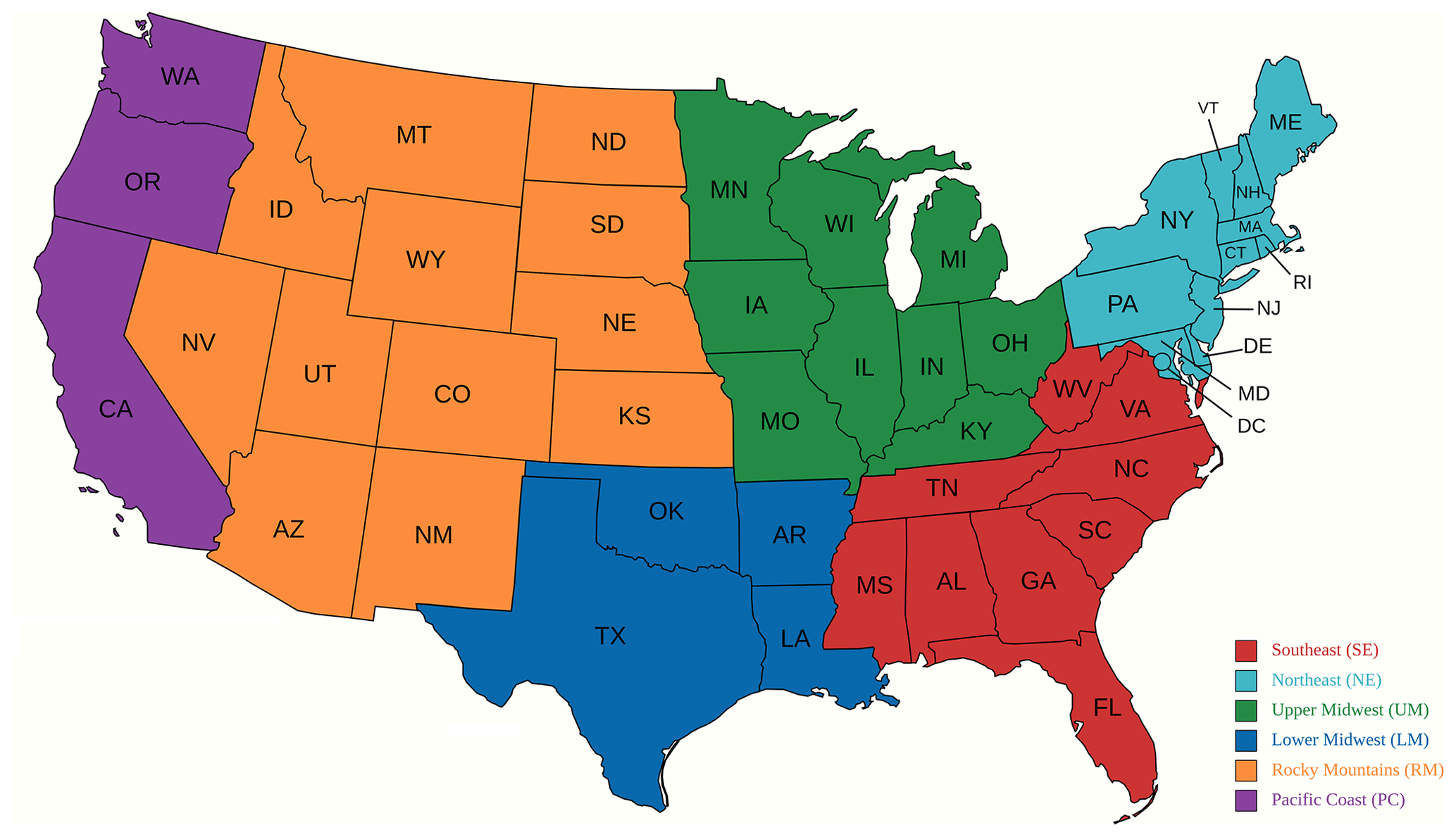
Figure 4 Geographical regions for statistical analysis.

Model-predicted ground-level ozone and NO_x concentrations were also compared to observations from the USEPA Air Quality System (AQS; https://www.epa.gov/aqs, last access: 24 November 2022). The commonly used evaluation metrics, including mean bias (MB), normalized mean bias (NMB), centered root mean square error (cRMSE), normalized mean error (NME), and correlation coefficient (R), were computed using the Atmospheric Model Evaluation Tool (AMET; Appel et al., 2011). The USEPA provides AMET-ready observation data from multiple networks, including the AQS, for the years 2000 through 2020 via the Community Modeling and Analysis System (CMAS) Center Data Warehouse (https://www.epa.gov/cmaq/atmospheric-model-evaluation-tool, last access: 10 August 2022), which greatly simplified the statistical analysis workflow of this study. Because lightning exhibits a substantial spatial and temporal variation (Kang and Pickering, 2018), the analysis was compiled for the entire model domain and different geographic regions shown in Fig. 4. The analysis regions follow Kang et al. (2019b) so that regional statistics obtained in this study can be compared to their results.

Table 5 Ground-level MDA8 ozone statistics over the model domain and geographic regions for August 2019. Bold numbers indicate better performance for each case. See Fig. 4 for the interpretation of geographical regions.

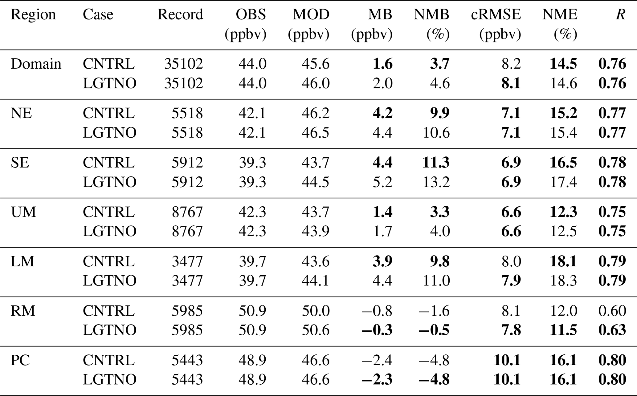
Table 6 Ground-level daily mean NO_x statistics over the model domain and geographic regions for August 2019. Bold numbers indicate better performance for each case. See Fig. 4 for the interpretation of geographical regions.

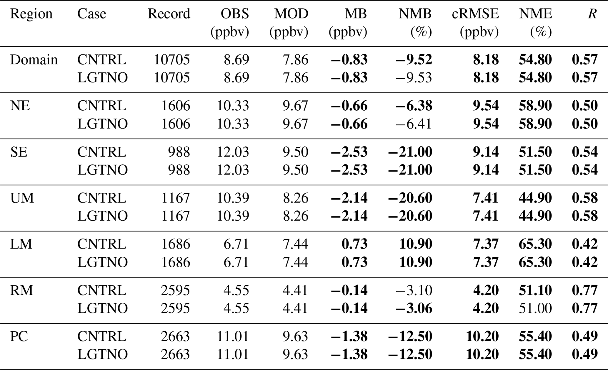
Tables 5 and 6 present statistics of maximum daily 8 h average (MDA8) ozone and daily mean NO_x for August 2019, respectively, when the percentage contribution of LNO emission to total NO_x emissions was the greatest among the simulation periods (Table 4). One caveat is that the statistical behavior discussed below may differ for other months because the predictive skill varies by month. Details on model performance for June, July, and September 2019 are provided in the Supplement (see Tables S3–S8). Generally speaking, the impact of LNO emission on ground-level ozone and NO_x was insignificant when averaged on a monthly scale. The difference in monthly mean concentrations was below 1 ppbv (or 2 % of the mean observed value) for MDA8 ozone and nearly negligible for daily mean NO_x. This is because most of the NO emission from lightning activity happens in the middle and upper troposphere. Only a small portion of LNO emission is released near the surface. Some recent studies (e.g., Kang et al., 2019b, 2020) also indicated that the average impact of LNO emission on ozone and NO_x is small at the ground level.

As shown in Table 5, the CNTRL simulation had slightly better MDA8 ozone statistics than the LGTNO for August 2019 in the northeast (NE), southeast (SE), upper Midwest (UM), and lower Midwest (LM), where the model overpredicted ground-level ozone concentrations. The situation was reversed in the Rocky Mountains (RM) and Pacific Coast (PC): ground-level ozone was underestimated in these regions, and statistics of the LGTNO simulation were slightly improved. This behavior indicates that the extra NO_x produced by lightning promotes ozone formation (unless the environment is VOC-limited, which may be the case in urban areas), increasing ozone biases when overpredicted and reducing when underpredicted. In addition, because lightning activity was prevalent in the SE and RM, changes in the mean bias and error were most significant in these two regions (Fig. 2). Table 6 demonstrates that ground-level NO_x mixing ratios were underestimated in most regions. Changes to the mean ground-level NO_x bias and error due to LNO emission at AQS sites were on the order of 0.1 ppbv (or 0.1 % after normalization), and the correlation was nearly unaffected. Despite this, NO_x statistics were marginally degraded in the NE, SE, and LM and improved in the RM, consistent with the performance of ground-level MDA8 ozone.

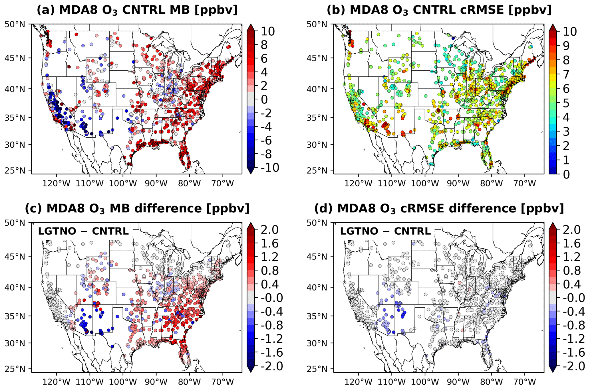
Figure 5 Spatial distribution of ground-level MDA8 ozone statistics for August 2019. (a) Mean bias of the CNTRL, (b) centered RMSE of the CNTRL, (c) absolute mean bias difference between the LGTNO and the CNTRL, (d) centered RMSE difference between the LGTNO and the CNTRL. In (c) and (d), negative and positive values represent improved and degraded statistics when including lightning NO emission, respectively.

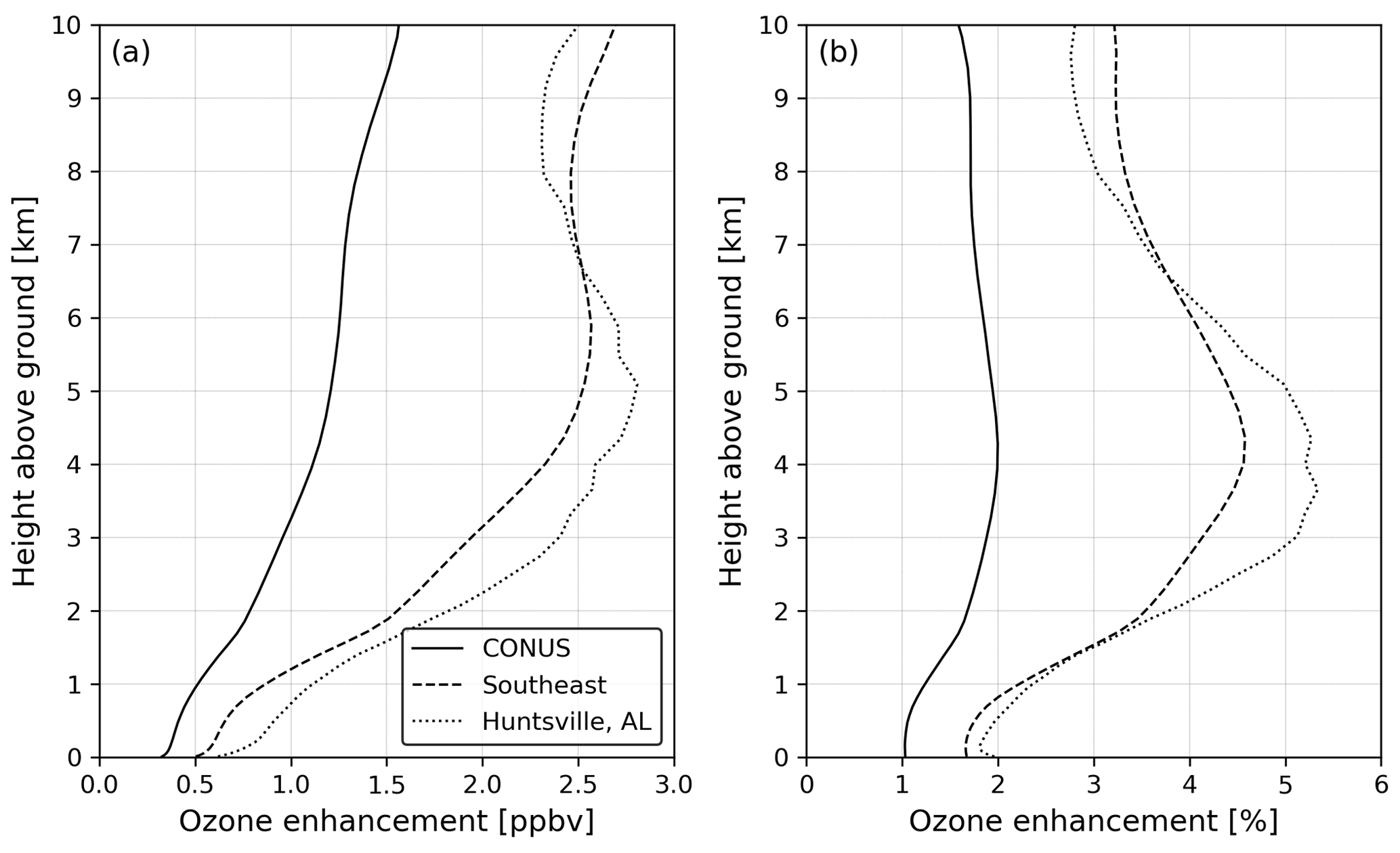
Figure 6 Vertical distribution of average ozone enhancement due to lightning NO_x emission during August 2019 for the CONUS domain; the southeastern US (arbitrarily selected as 25–40^∘ N, 75–95^∘ W for computation); and Huntsville, AL. (a) Ozone enhancement in ppbv, (b) ozone enhancement in percent.

Figure 5 presents the impact of LNO emission on ground-level MDA8 ozone at each AQS site during August 2019. For completeness, ground-level MDA8 ozone statistics during June, July, and September 2019 are provided in the Supplement (see Figs. S2–S4). In the CNTRL simulation, ground-level ozone tended to be overpredicted in the eastern US and underpredicted in the western US. Adding LNO emission to the simulation noticeably affected ozone statistics in the SE and RM. Also, since ground-level ozone was negatively biased in the RM and positively biased in the SE, the LGTNO simulation improved the prediction of ozone concentrations in the RM (especially in Arizona and New Mexico) but degraded in the SE. However, the difference between the absolute MB of the two simulations was below 2 ppbv, while the difference could reach up to 4 ppbv when the hNLDN scheme was used (Kang et al., 2019b). As mentioned earlier, this study used a lower (average) LNO production rate (i.e., $\stackrel{\mathrm{‾}}{P}=\mathrm{250}$ mol per flash) than Kang et al. (2019b), which is likely why a lower impact of LNO on ground-level air quality was obtained in this study. Since the LNO production rate is still highly uncertain, a more accurate estimate of the LNO emission will require a proper constraint on the tropospheric NO₂ column, which can be addressed in future studies using NO₂ observations from the NASA Tropospheric Emissions: Monitoring of Pollution (TEMPO; Zoogman et al., 2017).

4.3 Ozone enhancement in the tropospheric column

Because a large portion of the LNO emission takes place in the free troposphere rather than near the surface (Pickering et al., 1998; Ott et al., 2010; Koshak et al., 2014a; Wang et al., 2015; Kang et al., 2019a, b; Wu et al., 2023), which results in ozone production with a longer residence time, it is expected that ozone enhancement due to LNO emission is more significant in the middle and upper troposphere than at the ground level. To investigate how the LNO emission affects ozone concentrations in the tropospheric column, vertical distributions of monthly mean ozone enhancement below 10 km above ground level (a.g.l.) were constructed for different regions, including the entire domain; the southeastern US (arbitrarily selected as 25–40^∘ N, 75–95^∘ W for computation); and Huntsville, AL. The result for August 2019 is presented in Fig. 6 and discussed below, whereas the results for the other months are provided in the Supplement (see Figs. S5–S7) to indicate the variation for different months. In August 2019, when averaged for the entire domain, LNO increased ozone concentration throughout the troposphere, with a maximum percentage enhancement of 2 % (or 1.1 ppbv) at ∼ 4 km a.g.l., which was about twice the percentage at the ground level (1 %, or 0.3 ppbv). The impact of LNO emission on tropospheric ozone was more significant in the southeastern US, where the average ozone enhancement at 4 km was 4.5 % (or 2.3 ppbv). At Huntsville, AL, a 5.3 % (or ∼ 2.6 ppbv) ozone increase was simulated at ∼ 3.6 km. However, these numbers are generally lower than in previous studies in which higher LNO production rates were implemented (e.g., Wang et al., 2015; Kang et al., 2019b).

Although average ozone enhancement due to LNO emission appears to be small, the impact of LNO can be much greater in certain instances. This is because the frequency and intensity of lightning vary significantly with time and location. Shortly after a significant lightning event, ozone concentration in the downwind direction could rise substantially. The Huntsville, AL, area was investigated to demonstrate the details of such scenarios.

The Rocket-city O₃ Quality Evaluation in the Troposphere (RO₃QET) lidar (Kuang et al., 2011, 2013), one of the eight systems of the Tropospheric Ozone Lidar Network (TOLNet; https://tolnet.larc.nasa.gov/, last access: 17 January 2023), is located on the campus of the University of Alabama in Huntsville. The RO₃QET is an ozone differential absorption lidar (DIAL) that operates at 289 and 299 nm wavelengths. It can provide continuous observations of ozone profiles below ∼ 10 km at a typical temporal resolution of 10 min with an uncertainty of less than 10 % (Kuang et al., 2011, 2013).

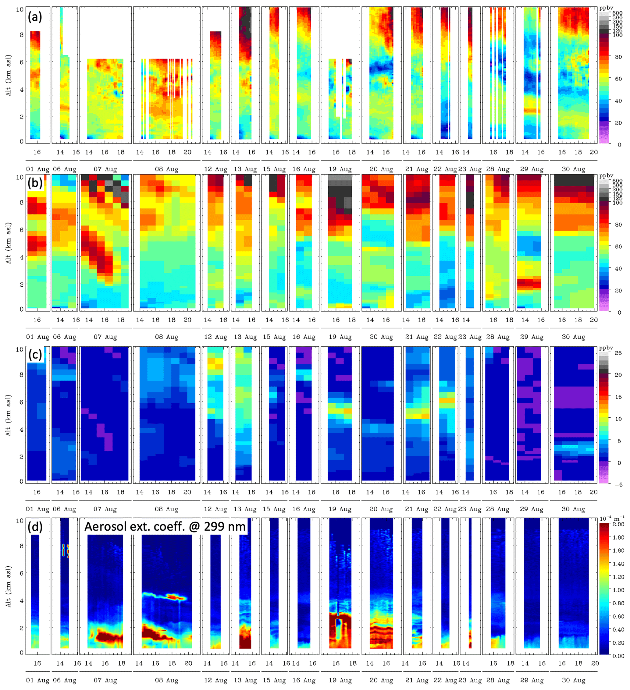
Figure 7 Time–height cross-sections of lidar-measured and model-simulated ozone mixing ratio at Huntsville, AL. (a) Lidar-measured ozone profiles, (b) simulated ozone mixing ratio by the CNTRL model run, (c) ozone difference between the LGTNO and the CNTRL, (d) lidar-observed aerosol extinction coefficient at 299 nm. All available lidar data in August 2019 and the corresponding model predictions are presented.

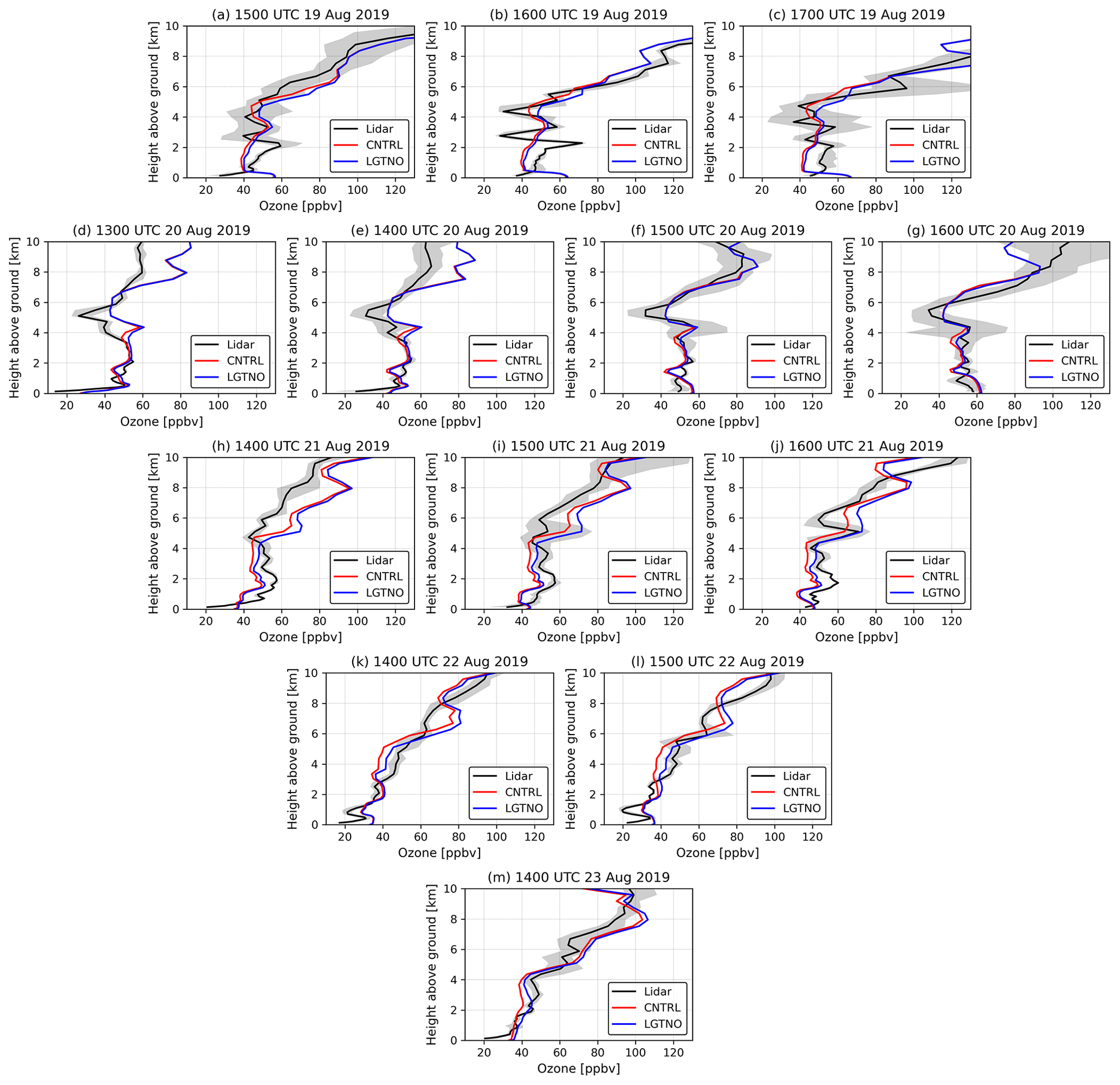
Figure 8 Hourly mean lidar-measured and model-simulated ozone profiles at Huntsville, AL, for all lidar observation periods between 19 and 23 August 2019. Black lines represent lidar observations after being averaged hourly and vertically to match the model resolution. Shaded regions indicate ranges of lidar measurements within each hour for each model layer. The red and blue lines represent model predictions of the CNTRL and the LGTNO, respectively.

By examining all available lidar measurements during the 2019 study period, it was realized that better temporal coverage was available in August. A model-to-lidar comparison was performed for all lidar operational periods in August 2019, and the results are presented in Fig. 7. One caveat is that optically thick aerosol layers were present on some days. Previous studies (e.g., Kuang et al., 2011, 2013, 2017) pointed out that heavy aerosol loading can strongly reduce lidar signal-to-noise ratios, resulting in degraded ozone retrievals. Therefore, caution should be taken when interpreting the results of the model-to-lidar comparison in such situations. Since lidar has a high vertical and temporal resolution, it can capture ozone gradients that the model may miss. Despite this, the pattern of model-simulated ozone concentrations was consistent with lidar measurements on most days, suggesting that model outputs can adequately represent the state of the atmosphere. During the investigated period, LNO emission caused significant (∼ 10 ppbv or more) ozone enhancements in the middle and upper troposphere on 12, 13, 19, 21, and 22 August 2019.

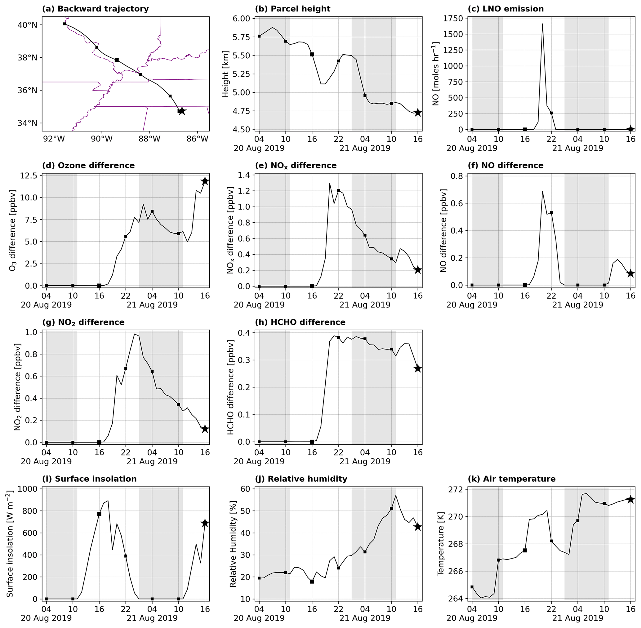
Figure 9 Backward trajectory analysis of the air mass that arrived at 34.724^∘ N, 86.645^∘ W (Huntsville, AL) at ∼ 4.7 km above ground level at 16:00 UTC on 21 August 2019. (a) Latitude and longitude, (b) parcel height, (c) hourly LNO emission, (d) ozone difference (between the LGTNO and the CNTRL), (e) NO_x difference, (f) NO difference, (g) NO₂ difference, (h) HCHO difference, (i) surface insolation, (j) relative humidity, and (k) air temperature along the trajectory. The squares indicate 6 h intervals along the trajectory. The star indicates the ending point of the trajectory. Shaded regions in the time series plots indicate local nighttime hours.

After taking a closer look at the difference between model-simulated and lidar-observed ozone mixing ratios, the 19–23 August 2019 period was chosen for further investigation. Figure 8 presents resolution-matched ozone profiles during this period. Lidar measurements were processed vertically to obtain averaged values for each model layer. Also, for each hour during which the lidar made multiple measurements, all 10 min lidar-measured ozone profiles within the hour were averaged. One may notice that model results did not always agree with the lidar observations. This is likely because model simulations were off by 1 h or so in time (or one grid cell or two in space). For example, at 13:00 UTC on 20 August 2019, the model did a fair job in the lower atmosphere and around 6 km but overpredicted ozone near 4–5.5 km and above ∼ 7 km. In the next few hours, lidar observations indicated a 10–25 ppbv ozone increase in the middle and upper troposphere, but the model did not show a significant temporal variation. As a result, model-simulated ozone agreed with lidar at 15:00 and 16:00 UTC, suggesting model predictions represented an air mass approximately 2 h ahead of the observation.

Among the hours presented in Fig. 8, the most significant tropospheric ozone enhancement due to LNO occurred at 16:00 UTC on 21 August 2019, with an increase of 11.8 ppbv at ∼ 4.7 km. To trace the source of this enhancement, NOAA's Hybrid Single-Particle Lagrangian Integrated Trajectory (HYSPLIT) model (Stein et al., 2015; https://www.ready.noaa.gov/HYSPLIT.php, last access: 19 January 2023) was executed to perform backward trajectory analysis. As shown in Fig. 9a and c, some lightning activity was observed near the boundary of Illinois and Kentucky at ∼ 20:00 UTC on 20 August 2019. The emitted LNO is mixed with the surrounding air when traveling southeastward. This results in increased ozone production in the air mass during daylight hours. As the ozone-enhanced (and NO_x-enhanced) plume reached the Huntsville area after 20 h transport, ozone concentration increased by more than 10 ppbv in the middle troposphere.

During the 2019 study period, the only field campaign providing ozone measurements was the Fire Influence on Regional to Global Environments and Air Quality (FIREX-AQ; https://www-air.larc.nasa.gov/missions/firex-aq/, last access: 23 January 2023). NASA Langley airborne High Spectral Resolution Lidar (HSRL; https://airbornescience.nasa.gov/instrument/HSRL, last access: 29 January 2023), carried by the NASA DC-8 instrument payload, actively remotely senses ozone and other species in the zenith and nadir directions along the flight path. A preliminary analysis indicated that, during the deployment days, lightning activity with more than 10 ppbv ozone enhancement was identified on 21, 23, and 26 August 2019 (see Figs. S8–S10 in the Supplement). In particular, Fig. S8 shows up to 15 ppbv ozone enhancements due to LNO on 21 August.

Since the significant lightning events are limited to a relatively small area within a short time period, ozone enhancement caused by LNO emission is also limited in time and space. This means that such enhancements can be significant but may not be evident when averaged over a much larger region and/or longer time. Thus, here we examine the maximum model-simulated tropospheric ozone enhancement caused by LNO emission. As demonstrated by Fig. 10, within the whole model domain, several regions showed ∼ 40 ppbv difference in ozone mixing ratio during the study period, most of which were over water bodies. The maximum ozone enhancement over the continental US was ∼ 38.6 ppbv, which occurred at 21:00 UTC on 29 June 2019 at 29.970^∘ N, 94.586^∘ W (located between Houston, TX, and Beaumont, TX). Performing backward trajectory analysis suggested that this significant ozone difference had two sources: (1) long-distance chemical transport and (2) lightning activity close to the event. Interestingly, this case was associated with the outflow boundary ahead of a southwestwardly moving mesoscale storm (https://www.wpc.ncep.noaa.gov/dailywxmap/index_20190629.html, last access: 25 January 2023).

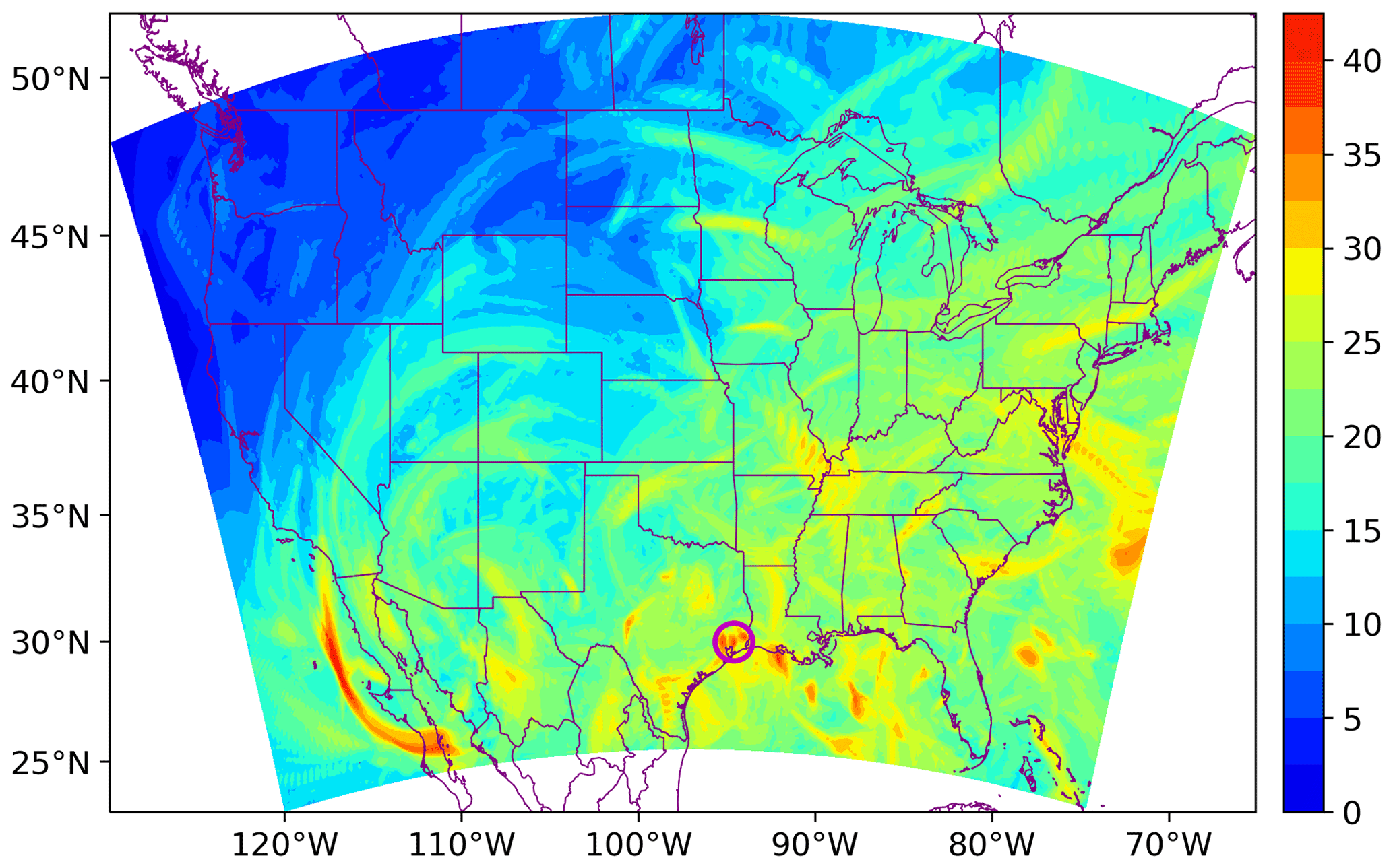
Figure 10 Spatial distribution of maximum ozone enhancement (entire simulation and all grid cells) within the troposphere due to LNO emission. The case of interest showing a ∼ 38.6 ppbv ozone increase occurred at 21:00 UTC on 29 June 2019 at 29.970^∘ N, 94.586^∘ W (located between Houston, TX, and Beaumont, TX, highlighted by the magenta circle) at ∼ 5.9 km above ground level.

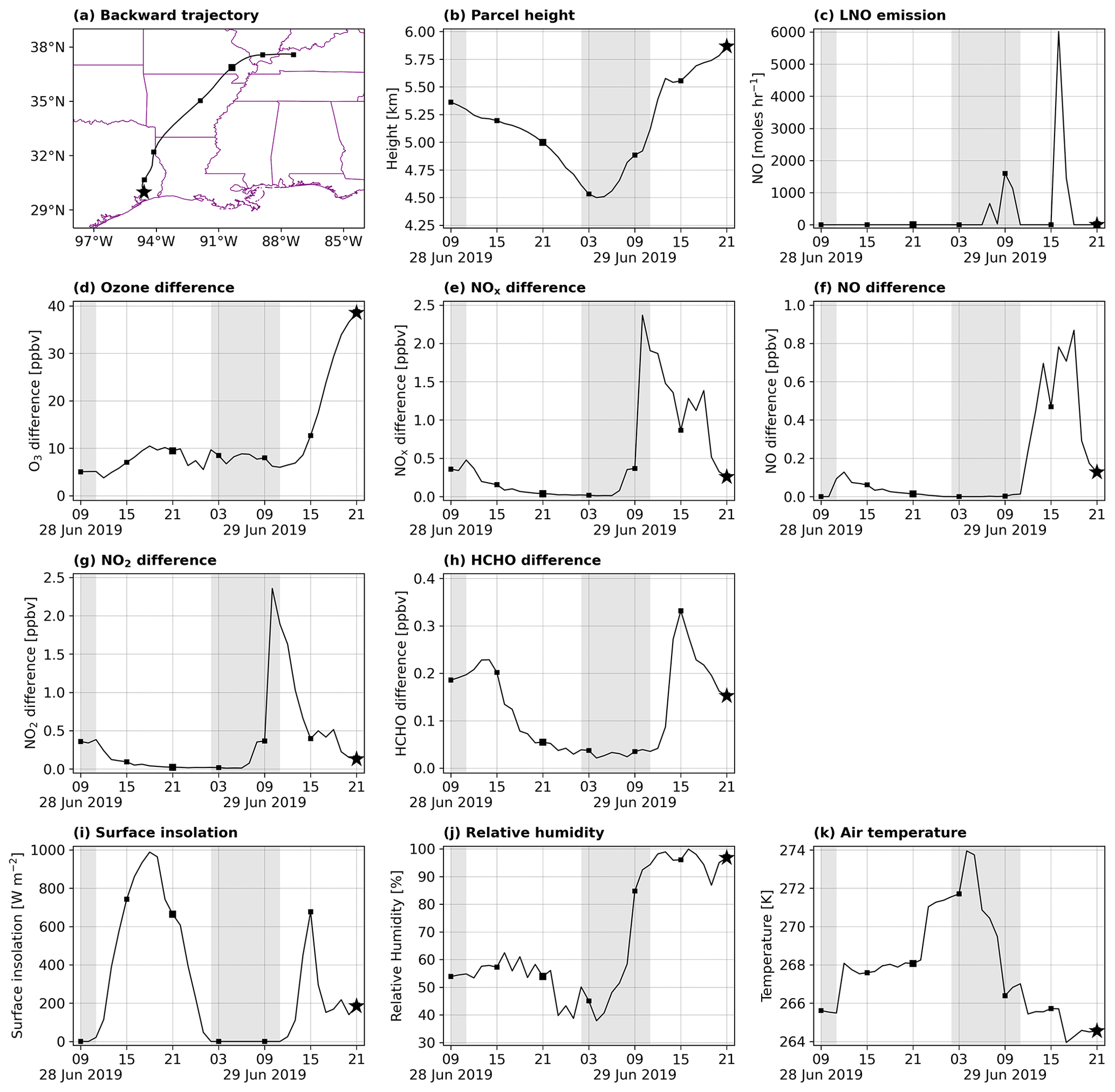
Figure 11 Backward trajectory analysis of the air mass that arrived at 29.970^∘ N, 94.586^∘ W (located between Houston, TX, and Beaumont, TX) at ∼ 5.9 km above ground level at 21:00 UTC on 29 June 2019. (a) Latitude and longitude, (b) parcel height, (c) hourly LNO emission, (d) ozone difference (between the LGTNO and the CNTRL), (e) NO_x difference, (f) NO difference, (g) NO₂ difference, (h) HCHO difference, (i) surface insolation, (j) relative humidity, and (k) air temperature along the trajectory. The squares indicate 6 h intervals along the trajectory. The star indicates the ending point of the trajectory. Shaded regions in the time series plots indicate local nighttime hours.

As illustrated by Fig. 11d, prior to 03:00 UTC on 29 August 2019 (22:00 CDT on 28 August 2019, local time) background ozone and NO_x in the upwind direction were higher in the LGTNO than in the CNTRL. This is perhaps due to the prior LNO emissions in the LGTNO simulation that causes approximately 5–10 ppbv of the ozone difference. The air mass altitude increases as it moves toward Houston, TX, and fresh LNO after this time (Fig. 11c) leads to another ∼ 30 ppbv ozone increase (Fig. 11d) by the time it is above Houston. Figure 10c indicates LNO emission over southwestern Arkansas and northwestern Louisiana after midnight and in southeastern Texas in the morning. The time series in Fig. 11 indicates that NO was first produced by lightning at night. Then, since there was no sunlight, the emitted NO was almost instantly oxidized by ozone and converted to NO₂. This is evident from the sharp NO₂ increase in Fig. 11g and the corresponding ozone reduction in Fig. 11d. Ozone concentration starts to increase shortly after sunrise, due to photochemistry and boundary layer mixing. Photochemical activity and the injection of additional LNO along the trajectory leads to a significant ozone increase (38.6 ppbv more than the CNTRL). In addition, surface insolation drops dramatically at the time of LNO emission during the day, suggesting that the model correctly produced clouds at locations where lightning flashes were observed.

An interesting feature in this trajectory is the chemical evolution of the air mass with respect to its location and the role of atmospheric dynamics (Parrish et al., 2012). Figure 11h shows a rapid increase in formaldehyde after sunrise up to 15:00 UTC. This increase is positively correlated with NO and negatively correlated with NO₂, indicating the presence of adequate VOC and a very active photochemistry. The elevation of the air mass is more than 5 km during this period. Thus, the VOC must have been transported from near-surface pollution in the Houston area. After 15:00 UTC, HCHO starts to decrease, while ozone continues to increase. The timing of the decrease coincides with the injection of fresh lightning NO. This is typical behavior of a NO_x-limited air mass. From the time series in Fig. 11, it can be deduced that prior to 15:00 UTC, as the clouds are forming, vertical transport of boundary layer air to higher altitudes increases VOC and creates a NO_x-limited chemical environment. This is evident by the decrease in NO_x, increase in HCHO, increase in relative humidity, and relatively lower surface insolation. However, after 15:00 UTC, with the injection of fresh LNO in this NO_x-limited air mass, rapid ozone production transpires. The rapid ozone production is being helped by the fact that at this time the air mass is higher up in the clouds and perhaps exposed to relatively higher actinic flux (Ryu et al., 2017).

5 Conclusions

This study is our first attempt to employ the LNO emission estimates derived from GLM spaceborne lightning observations in air quality model simulations. Our results showed that, for the CONUS domain, lightning activity released approximately 0.174 Tg N of NO into the atmosphere between June and September 2019, accounting for 11.4 % of the total NO_x budget over this area. Performing two CMAQ simulations revealed that adding the GLM-based LNO emission increased ozone concentration within the troposphere (below 10 km a.g.l.) in August 2019 by a domain-wide average of 1 %–2 % (or 0.3–1.5 ppbv), with the maximum enhancement at ∼ 4 km a.g.l. and the minimum near the surface. The strength and frequency of lightning events are unevenly distributed across the CONUS, and so is the impact of LNO emission on ozone concentration. Due to relatively more lightning and biogenic VOC in the southeastern US, this region exhibited the most significant difference in ground-level ozone, with up to 1 ppbv (or 2 % of the mean observed value) increase for MDA8 ozone. However, although the numbers above generally fall within the uncertainty range given in previous studies, many are closer to the lower bound. This is partially due to using a smaller average LNO production rate (i.e., $\stackrel{\mathrm{‾}}{P}=\mathrm{250}$ mol NO per flash) in the estimation of β in this study compared to other recent studies (Kang et al., 2019a, 2020). It is important to note that although this work assumes a fixed value of the average LNO production rate per flash, the β method employed still assigns distinct LNO production values to each flash in general, based directly on the variable/unique GLM flash-optical-energy observations. It is also important to note that we have not corrected for GLM flash detection efficiency (DE) which varies significantly; i.e., roughly 20 %–95 % across CONUS for both GLM-16 and GLM-17 (Katrina Virts and William Koshak, personal communications, 2023, based on their Bayesian DE analyses). Not correcting for the DE contributes to underestimation of LNO emissions (and its impact on ozone). Studies are currently in progress to finalize the GLM-16/GLM-17 and GLM-18 DE estimates for applications in future air chemistry studies.

While the average influence of LNO on tropospheric ozone over the entire study period was small, the local impact on a shorter timescale could be considerable. The LGTNO simulation at Huntsville, AL, agreed with the hourly averaged ozone lidar observations in general, despite some discrepancies due to the different temporal resolutions. The results of backward trajectory analyses illustrated that long-range chemical transport and upwind lightning activity are the two major contributing factors for significant ozone enhancement. A case study was presented, exhibiting a tropospheric ozone enhancement of 38.6 ppbv over Houston, TX. Trajectory analysis demonstrated that during the formation of storms, boundary layer air that is rich in VOC can be transported to higher altitudes and diluted to create a NO_x-limited environment. In such an environment, the addition of fresh NO from lightning can lead to significant ozone production. Furthermore, storms provide a mechanism for the transport of higher-tropospheric LNO to the surface and the transport of boundary layer air to higher altitudes.

In future studies, potential improvements are expected after making proper adjustments. As indicated, the average LNO emission rate in this study is on the lower end of the estimates and could be increased for the follow-up studies. A more accurate LNO production rate can be obtained by constraining tropospheric NO_x columns based on geostationary (e.g., TEMPO) satellite observations. Also, implementing cloud/lightning data assimilation techniques can reduce the temporal and spatial discrepancy between model-simulated clouds and GLM-captured lightning flashes. Moreover, as this study focuses mainly on the impact of GLM-derived LNO emission on ozone-related gas-phase photochemistry, it would be interesting to investigate how the LNO emission affects particulate matter, particularly wet and dry depositions of aerosol nitrates (NO${}_{\mathrm{3}}^{-}$), which is another often-studied area in the literature (e.g., Kang et al., 2022b).