Measurement report: Assessing the impacts of emission uncertainty on aerosol optical properties and radiative forcing from biomass burning in peninsular Southeast Asia

Despite significant advancements in improving the dataset for biomass burning (BB) emissions over the past few decades, uncertainties persist in BB aerosol emissions, impeding the accurate assessment of simulated aerosol optical properties (AOPs) and direct radiative forcing (DRF) during wildfire events in global and regional models. This study assessed AOPs (including aerosol optical depth (AOD), aerosol absorption optical depth (AAOD), and aerosol extinction coefficients (AECs)) and DRF using eight independent BB emission inventories applied to the Weather Research and Forecasting model coupled with Chemistry (WRF-Chem) during the BB period (March 2019) in peninsular Southeast Asia (PSEA), where the eight BB emission inventories were the Global Fire Emissions Database version 4.1s (GFED), Fire INventory from NCAR version 1.5 (FINN1.5), the Fire Inventory from NCAR version 2.5 MOS (MODIS fire detections; FINN2.5 MOS), the Fire Inventory from NCAR version 2.5 MOSVIS (MODIS + VIIRS fire detections; FINN2.5 MOSVIS), Global Fire Assimilation System version 1.2s (GFAS), Fire Energetics and Emissions Research version 1.0 (FEER), Quick Fire Emissions Dataset version 2.5 release 1 (QFED), and Integrated Monitoring and Modelling System for Wildland FIRES project version 2.0 (IS4FIRES), respectively. The results show that in the PSEA region, organic carbon (OC) emissions in the eight BB emission inventories differ by a factor of about 9 (0.295–2.533 Tg M⁻¹), with 1.09 ± 0.83 Tg M⁻¹ and a coefficient of variation (CV) of 76 %. High-concentration OC emissions occurred primarily in savanna and agricultural fires. The OC emissions from the GFED and GFAS are significantly lower than the other inventories. The OC emissions in FINN2.5 MOSVIS are approximately twice as high as those in FINN1.5. Sensitivity analysis of AOD simulated by WRF-Chem to different BB emission datasets indicated that the FINN scenarios (v1.5 and 2.5) significantly overestimate AOD compared to observation (VIIRS), while the other inventories underestimate AOD in the high-AOD (HAOD; AOD > 1) regions range from 15–22.5^∘ N, 97–110^∘ E. Among the eight schemes, IS4FIRES and FINN1.5 performed better in terms of AOD simulation consistency and bias in the HAOD region when compared to AERONET sites. The AAOD in WRF-Chem during the PSEA wildfire period was assessed, using satellite observations (TROPOMI) and AERONET data, and it was found that the AAOD simulated with different BB schemes did not perform as well as the AOD. The significant overestimation of AAOD by FINN (v1.5 and 2.5), FEER, and IS4FIRES schemes in the HAOD region, with the largest overestimation for FINN2.5 MOSVIS. FINN1.5 schemes performed better in representing AAOD at AERONET sites within the HAOD region. The simulated AOD and AAOD from FINN2.5 MOSVIS always show the best correlation with the observations. AECs simulated by WRF-Chem with all the eight BB schemes trends were consistent with CALIPSO in the vertical direction (0.5 to 4 km), demonstrating the efficacy of the smoke plume rise model used in WRF-Chem to simulate smoke plume heights. However, the FINN (v1.5 and 2.5) schemes overestimated AECs, while the other schemes underestimated it. In the HAOD region, BB aerosols exhibited a daytime shortwave radiative forcing of −32.60 ± 24.50 W m⁻² at the surface, positive forcing (1.70 ± 1.40 W m⁻²) in the atmosphere, and negative forcing (−30.89 ± 23.6 W m⁻²) at the top of the atmosphere. Based on the analysis, FINN1.5 and IS4FIRES are recommended for accurately assessing the impact of BB on air quality and climate in the PSEA region.

1 Introduction

Peninsular Southeast Asia (PSEA), including Vietnam, Thailand, Myanmar, Cambodia, and Laos, is one of the major biomass burning (BB) emission source areas in the world (Yadav et al., 2017). Due to widespread forest fires and agro-residue burning, extensive BB activities occur over PSEA, especially during the dry season (BB usually peaks in March) (Reddington et al., 2021) and release large amounts of aerosols and trace gases (including organic carbon (OC), black carbon (BC), particulate matter (PM), nitrogen oxides (NO_x), and volatile organic compounds (VOCs)) into the air, thus leading to significant impacts on atmospheric composition, radiative budget, and human health (Reid et al., 2013). Therefore, it is crucial to understand the BB emission inventories, as well as the behavior of aerosols, and accurately model their properties to assess their impact on air quality and climate change in the PSEA region.

Numerous studies have been conducted to assess the effects of BB emissions on aerosol optical properties (AOPs), such as aerosol optical depth (AOD), absorbing aerosol optical depth (AAOD), and aerosol extinction coefficient (AEC), as well as direct radiative forcing (DRF) in the PSEA region (Zhu et al., 2017; Lin et al., 2014; Dong and Fu, 2015b). However, most of these studies have relied on only one single BB emission inventory, without comparing different inventories, leading to large uncertainties in assessing the impact of BB aerosols. Due to the challenges in directly measuring BB emissions, various global fire emission inventories have been developed, based on satellite observations, in the past decades (Ichoku and Ellison, 2014; Wiedinmyer et al., 2023; Wiedinmyer et al., 2011). These inventories use different empirical methods and underlying data to represent gas and aerosol emissions from fires, resulting in inherent uncertainties (Carter et al., 2020).

These uncertainties arising from different BB emissions often manifest as regional variations and inconsistencies with observations when integrated into models (Liu et al., 2020). Addressing these uncertainties is crucial for refining climate models and providing more accurate projections of future climate change. For example, Pan et al. (2020) compared six BB aerosol emission datasets from 2008 globally, as well as from 14 regions, and the total global emissions from these BB emission datasets differed by a factor of 3.8. Sensitivity analysis of AOD simulated by Goddard Earth Observing System with Chemistry (GEOS-Chem) to different BB emission datasets during the peak BB period in each region and at most AERONET (AErosol RObotic NETwork) sites in each region found that the Quick Fire Emissions Dataset version 2.4 (QFED2.4) produced the highest AOD values, closest to observations, followed closely by Fire Energetics and Emissions Research version 1.0 (FEER1.0). In the North American region, GEOS-Chem, incorporating four different BB emission inventories and remote-sensing data analysis during wildfire periods, indicated a 4–7-fold difference in BB aerosol emissions. Simulations driven by Global Fire Emissions Database version 4s (GFED4s) and Global Fire Assimilation System version 1.2 (GFAS1.2) provide better agreement with surface measurements of organic aerosol and BC mass concentrations, BC observations at higher altitudes, and Moderate Resolution Imaging Spectroradiometer (MODIS) observations of AOD (Carter et al., 2020). To explore the uncertainty of BB emissions in the tropics, GFED V3, Fire INventory from NCAR version 1 (FINN1.0), and GFAS1 were used to evaluate Global Model of Aerosol Processes (GLOMAP) model simulations of AOD in South America, Africa, and Southeast Asia, showing that the model underestimates AOD for all emission datasets (Reddington et al., 2016). In the northern sub-Saharan Africa BB region, Zhang et al. (2014) found a 12-fold difference in estimates of total smoke emissions and an even larger difference (up to 33-fold) in Weather Research and Forecasting model coupled with Chemistry (WRF-Chem)-simulated smoke-related variables and radiative effects. Wiedinmyer et al. (2023) have shown that the seasonal cycle (averaged over 2012–2019) of CO emissions from BB in various regions of the world and the latest version of FINN v2.5 (MODIS + VIIRS) has an emission peak in March, primarily driven by emissions from the PSEA. However, this peak is absent in GFED and is less pronounced in other emission inventories (FINN1.5, FEER, GFAS, and QFED). Despite substantial research efforts, accurately representing BB aerosols in models remains a challenge. In summary, compared to the differences between global BB emission inventories, regional differences may be larger, especially in the PSEA region, where the satellite inversions of BB contain a large fraction of uncertainty due to high-cloud cover (Dong and Fu, 2015a). Significant differences exist in AOPs and radiative forcing simulated by different emission inventories in the BB high-emission region within a single model (Carter et al., 2020; Zhang et al., 2014). To reduce uncertainties, it is necessary to compare the differences between commonly used BB emission inventories and evaluate the model simulations of AOPs and radiative effects for the PSEA region.

The World Meteorological Organization's report highlights that the early part of 2019 corresponds to the El Niño phase of the El Niño–Southern Oscillation (ENSO) cycle (from April to May, the temperature of waters beneath the surface of the tropical Pacific has notably declined) (World Meteorological Organization, 2019), during which meteorological conditions are more favorable for the occurrence and propagation of BB (Cochrane, 2009). Additionally, Yin (2020) discovered that over the past 18 years (2001–2018), the PSEA region predominantly experienced the peak of BB activity in March each year. Fan et al. (2023) and Duc et al. (2021) confirmed that the PSEA suffered severe air quality impacts during the BB in March 2019. Therefore, centered on the period of March 2019, this study aims to analyze how emission uncertainties or differences from different BB inventories affect the spatial and temporal distribution of aerosols and their radiative effects in the PSEA region. Section 2 describes the model configuration, experimental design, and data sources. Section 3 presents a comparison of eight emission inventories in March 2019 and the results of simulating AOPs and DRF. A discussion is provided in Sect. 4, and the study concludes with a summary in Sect. 5.

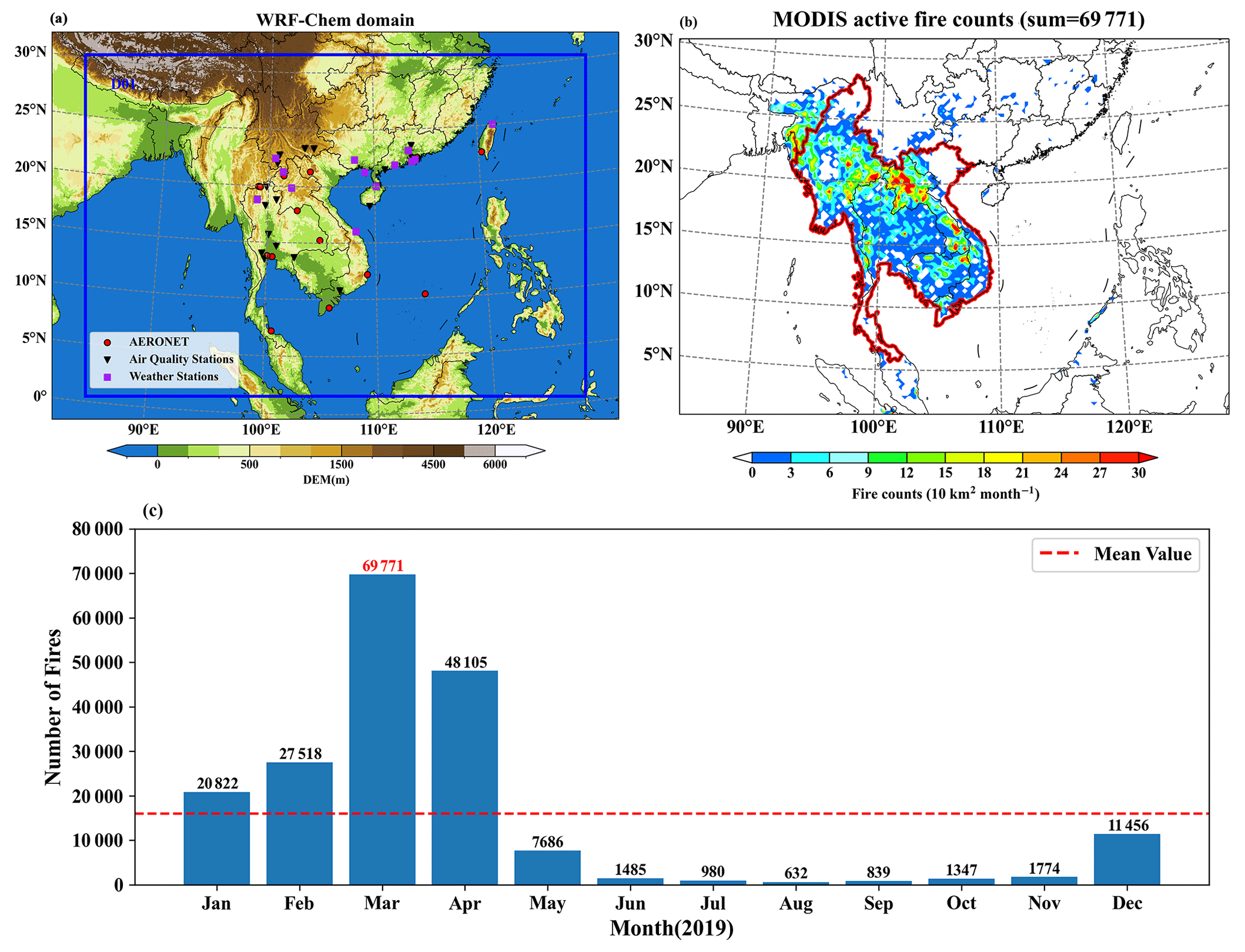
Figure 1 (a) WRF-Chem simulation domain (D01; blue line), topography based on the digital elevation model (DEM), and observation stations, where the red dots are AERONET stations, the black triangles are air quality stations, and the purple rectangles are meteorological stations. (b) Spatial distribution characteristics of fire points in PSEA (red line; including Vietnam, Thailand, Myanmar, Cambodia, and Laos) from MODIS satellite retrieval in March 2019. (c) Total fire counts in the PSEA region from January to December 2019 (MODIS). Publisher's remark: please note that Figs. 1a and b, 3, 5, 6, 9, 10, and 13 contain disputed territories.

2 Data and methods

2.1 Model description and configuration

2.1.1 WRF-Chem

The simulations were conducted using version 3.9.1.1 of the WRF-Chem online coupled meteorology and chemistry model (Grell et al., 2005). Figure 1 depicts the simulation domain, which is outlined in blue (Fig. 1a). It shows that the MODIS active fire instances during March 2019 were primarily consolidated in Laos, Cambodia, and northern Thailand, as well as in eastern and western Myanmar (Fig. 1b). Importantly, with a total of 69 771 fire counts, March 2019 saw the highest monthly peak of fires for that year (Fig. 1c). The simulation period is from 26 February to 31 March 2019, where the initial 3 d of the model simulation were used as a spin-up period. The model consisted of 27 vertical layers and one nested horizontal resolution of 27 km × 27 km. The selected physical configurations included the Morrison double-moment microphysics scheme (Morrison et al., 2005), the rapid radiation transfer model (RRTMG) longwave and shortwave radiation schemes (Iacono et al., 2008), the Mellor–Yamada–Janjić (MYJ) planetary boundary layer scheme (Mellor and Yamada, 1982; Janjiæ, 1990), the Eta-similarity surface layer scheme (Monin and Obukhov, 1954), the Noah land surface model land surface scheme (Niu et al., 2011), and the Grell 3D cumulus parameterization scheme (Grell and Dévényi, 2002). The Model for Ozone and Related chemical Tracers (MOZART) trace gas chemistry with the Model for Simulating Aerosol Interactions and Chemistry (MOSAIC; with four bins) aerosol scheme with the kinetic preprocessor (KPP) library is used in the model (Emmons et al., 2010). In this study, MOSAIC uses a sectional approach to represent aerosol size distributions with four discrete size bins with glyoxal uptake into aqueous aerosols to form secondary organic aerosol (SOA) in the PSEA region by WRF-Chem; this is capable of simulating all major aerosol components, including nitrates (${\mathrm{NO}}_{\mathrm{3}}^{-}$), sulfates (${\mathrm{SO}}_{\mathrm{4}}^{-\mathrm{2}}$), ammonium (${\mathrm{NH}}_{\mathrm{4}}^{+}$), BC, primary organic aerosols, and other inorganic aerosols through a thermodynamic approach, with high efficiency and accuracy for use in air quality and regional and/or global aerosol modeling (Zhang et al., 2018). The aerosol–radiation interaction (ARI) scheme of WRF-Chem includes the traditional aerosol direct and semi-direct effects (Baró et al., 2016). Mallet et al. (2020) and Palacios-Peña et al. (2018) found that model incorporation of ARI can effectively replicate smoke aerosol simulations, so the ARI scheme was selected for this paper. The Community Atmosphere Model with Chemistry (CAM-chem) simulation outputs (Emmons et al., 2020; Buchholz et al., 2019) are used as chemical lateral boundary and initial conditions for WRF-Chem (https://rda.ucar.edu/datasets/ds313.7/, last access: 11 May 2023). The product simulated by CAM-chem has a horizontal resolution of 0.9^∘ by 1.25^∘ and 56 vertical levels in the vertical direction. Meteorological initial and boundary conditions were obtained from the National Centers for Environmental Prediction (NCEP) final analysis data, with a 1^∘ × 1^∘ horizontal resolution.

WRF-Chem employs Mie theory to perform calculations of AOPs, using MOSAIC size distributions and the complex refractive indices associated with each MOSAIC chemical constituent. Specifically, it simulates AOPs (such as AEC, single-scattering albedo (SSA), and asymmetry factor for scattering) distributed in the following four different bands: 300, 400, 600, and 1000 nm. This study used the Ångström power law (Ångström, 1929; Martýnez-Lozano et al., 1998) to derive the model at 550 nm for AOD, and the detailed calculation procedure follows Kumar et al. (2014) and Saide et al. (2013). In addition, the aerosol direct radiative feedback was coupled with the RRTMG for both shortwave (SW) and longwave (LW) radiation, as implemented by Zhao et al. (2010). A detailed description of the computation of AOPs and DRF in WRF-Chem has been given by Fast et al. (2006), Zhao et al. (2011), and Lin et al. (2014).

2.1.2 Anthropogenic and biogenic emissions

The latest version of the global anthropogenic emission inventory, the monthly Emissions Database for Global Atmospheric Research (EDGAR) v5.0, was published on 17 February 2022 (Mogno and Marvin, 2022). It provides global air pollutant emissions for the year 2015 at a resolution of 0.1^∘ × 0.1^∘. These emissions were speciated for the MOZART chemical mechanism and can be accessed at https://zenodo.org/record/6130621 (last access: 11 May 2023). Biogenic emissions were calculated online within the model, using the Model of Emissions of Gases and Aerosols from Nature (MEGAN) inventory developed by Guenther et al. (2012).

Table 1 Comprehensive comparison of eight BB emission inventories globally in terms of different methodological details and species, where a bottom-up approach to construct emission inventories is found in GFED v4.1s, FINN v1.5, FINN v2.5 MOS, and FINN v2.5 MOSVIS, while others make use of a top-down approach.

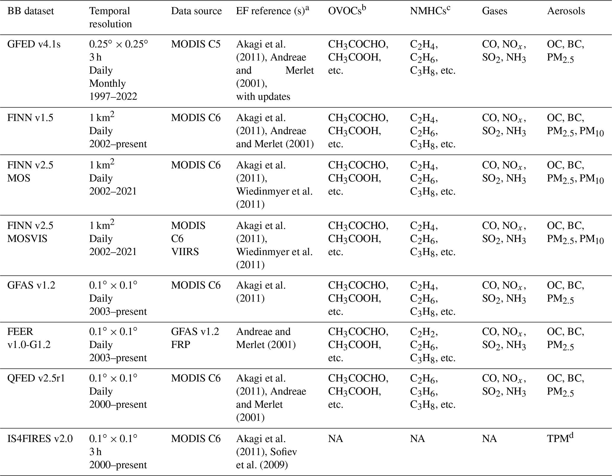
^a The main references for emission factors (EFs) used in the BB emission database. ^b Oxygenated volatile organic compounds (OVOCs) contain C, H, and O. Examples include alcohols, aldehydes, ketones, and organic acids. ^c Non-methane hydrocarbons (NMHCs) are defined as organic compounds, excluding methane (CH₄), that contain only C and H. ^d The total particle matter (TPM) considers three different particle sizes (0.17, 1.1, and 3 µm). Note that OVOCs and NMHCs together account for nearly all the gas-phase non-methane volatile organic compounds (NMVOCs) emitted by fires (Akagi et al., 2011). NA stands for not available.

2.2 BB emission inventories

There are two primary approaches to estimating BB emission inventories, namely “bottom-up” and “top-down” methods (Archer-Nicholls et al., 2015). The bottom-up approach involves estimating emissions per species by multiplying emission factors (EFs) with estimates of the biomass burned (Yevich and Logan, 2003). The latter, the top-down approach, bypasses the largely uncertain fuel consumption estimation step by estimating emission fluxes directly from fire radiative power (FRP) (Ichoku and Ellison, 2014). The top-down approach commonly utilizes AOD retrieved from satellite remote sensing to constrain aerosol emissions from wildfires (Huneeus et al., 2012). This study evaluates the performance of the WRF-Chem using eight different BB emission inventories to simulate wildfires in the PSEA region during March 2019. These emission inventories include the Global Fire Emissions Database version 4.1s (GFED), Fire INventory from NCAR version 1.5 (FINN1.5), the Fire Inventory from NCAR version 2.5 MOS (MODIS fire detections; FINN2.5 MOS), the Fire Inventory from NCAR version 2.5 MOSVIS (MODIS + VIIRS fire detections; FINN2.5 MOSVIS), Global Fire Assimilation System version 1.2s (GFAS), Fire Energetics and Emissions Research version 1.0 (FEER), Quick Fire Emissions Dataset version 2.5 release 1 (QFED), and Integrated Monitoring and Modelling System for Wildland FIRES project version 2.0 (IS4FIRES). Table 1 provides a detailed comparison of their spatial and temporal resolution, the main references for the EFs, the satellite data sources, non-methane hydrocarbons (NMHCs), oxygen volatile organic compounds (OVOCs), gases (CO, NO_X, SO₂, and NH₃), and aerosols in the inventory. NMHCs refer to organic compounds containing only C and H, besides methane (CH₄), such as alkanes, alkenes, and alkynes. OVOCs contain C, H, and O compounds (e.g., alcohols, aldehydes, and ketones). NMHCs and OVOCs combined constitute nearly all of the non-methane volatile organic compounds (NMVOCs) emitted by wildfires (Akagi et al., 2011).

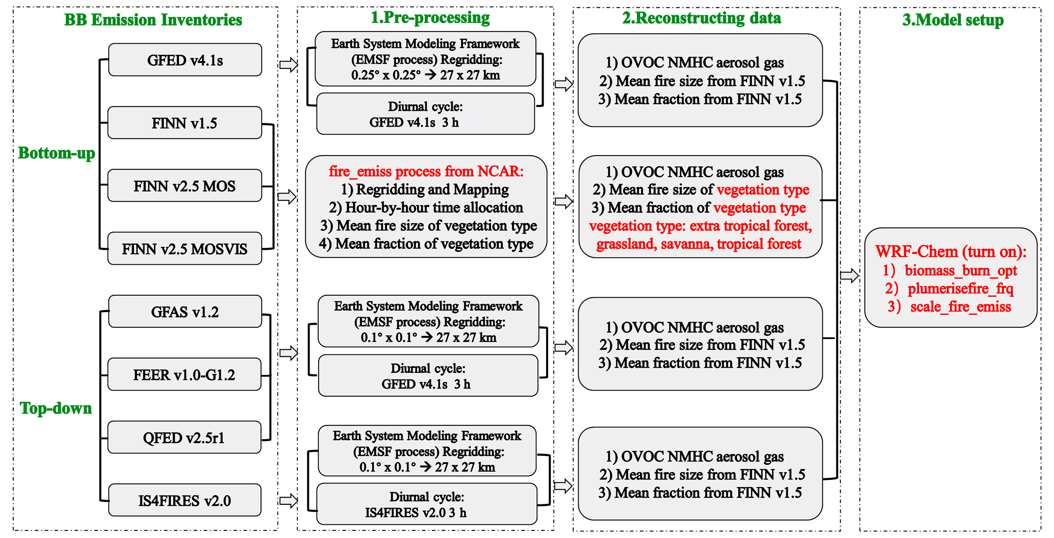
Figure 2 The flowchart illustrates the three processes of pre-processing, reconstructing data, and model setup to put the eight BB emission inventories into the WRF-Chem simulation of AOPs and DRFs during the March 2019 wildfires in the PSEA region. Pre-processing consisted of regridding and time allocation, where the FINN scenario was processed using the fire_emiss program from NCAR, while the grids generated by the other scenarios based on the FINN 1.5 scenario were spatially allocated using the Earth System Modeling Framework (EMSF) program. GFED, GFAS, FEER, and QFED have the same time allocations as GFED, and the remainder use self-contained time allocations. The reconstructing data have three components, namely emissions (OVOCs, NMHCs, aerosol, and gas) composed by the MOZART–MOSAIC mechanism, fire size, and vegetation proportions (extratropical forest, grassland, savanna, and tropical forest). Compared to the FINN schemes, the missing compounds and aerosols from the other schemes were added based on the methodology of Jose et al. (2017) and Andreae and Merlet (2001; 2019). Eight BB emission inventories used the fire sizes provided by the FINN 1.5 scheme, as well as the vegetation proportions. The model setup turned on BB simulations including the smoke plume rise.

2.2.1 GFED (v4.1s)

The GFED4.1s datasets provide the area burned, dry matter (DM), and EFs from global fires. It has a spatial resolution of 0.25^∘∘0.25^∘ and can be accessed at https://daac.ornl.gov/get_data/ (last access: 11 May 2023). This dataset includes fractional contributions from different fire types and offers daily or 3 h data to scale monthly emissions to a higher temporal resolution. GFED4.1s is an enhanced version of the GFED4 dataset, incorporating small fire inputs to enhance the accuracy and completeness of emission estimates (Randerson et al., 2017). It covers the period from June 1997 to 2022 and includes a wide range of emission species such as carbon (C), DM, carbon dioxide (CO₂), carbon monoxide (CO), methane (CH₄), hydrogen (H₂), nitrous oxide (N₂O), NO_x, NMHCs, OVOCs, OC, BC, PM less than 2.5 µm in diameter (PM_2.5), total PM (TPM), and sulfur dioxide (SO₂). The raw GFED emission data (0.25^∘ × 0.25^∘) were first regridded to the required spatial resolution for the WRF-Chem domains using the Earth System Modeling Framework (EMSF) program in Fig. 2, followed by supplementing the GFED emission species (Table S1 in the Supplement) to meet the MOZART–MOSAIC scheme, based on the study by Akagi et al. (2011) and Heil and Bouarar (2020). The construction of the final emission inventory included incorporating the mean fraction and fire size of the four vegetation types (grassland, extratropical forest, savanna, and tropical forest) from FINN1.5. This incorporation enables WRF-Chem to calculate the smoke plume rise (Freitas et al., 2007, 2010).

2.2.2 FINN (v1.5 and v2.5 MOS and v2.5 MOSVIS)

The emissions estimation of FINN (v1.5 and 2.5) is based on the framework described by Wiedinmyer et al. (2011, 2023), which utilizes the following two types of satellite observations: (1) MODIS fire detections and (2) active fire detections from both MODIS and the Visible Infrared Imaging Radiometer Suite (VIIRS). It provides global daily estimates of BB emissions for important gases and aerosols, along with comprehensive specifications of total VOC emissions for three commonly used chemical mechanisms (MOZART-T1, SAPRC99, and GEOS-Chem) in regional and global chemical transport models (https://www.acom.ucar.edu/Data/fire/, last access: 11 May 2023). Since its release, FINN has been widely utilized by researchers to assess air quality during wildfire events (Lin et al., 2014; Vongruang et al., 2017; Pan et al., 2020). The latest version, FINN v2.5, was introduced in 2022 and incorporates an updated algorithm for determining fire size by aggregating adjacent fire detections. Compared to FINN1.5, FINN2.5 incorporates significant improvements in input data and processing methods for detecting fire activity, characterizing annual land use/land cover and vegetation density, estimating burned area, and applying fuel loads across different global regions (Wiedinmyer et al., 2023). In this study, FINN1.5 and FINN2.5 MOS (MODIS-only fire detections) and FINN2.5 MOSVIS (MODIS + VIIRS fire detections) were used. Detailed information on emission species and factors can be found in Tables S2 and S3.

2.2.3 GFAS (v1.2)

GFAS provides data outputs that encompass spatially gridded FRP, DM burning, and BB emissions for numerous chemical, greenhouse gas, and aerosol species (Andela et al., 2013). These data are globally available from 2003 to the present, with a regular latitude and longitude grid resolution of 0.1^∘ × 0.1^∘ (https://ads.atmosphere.copernicus.eu/cdsapp#!/dataset/cams-global-fire-emissions-gfas, last access: 11 May 2023). The latest version, GFAS 1.2, includes injection height daily data (mean altitude of maximum injection and altitude of plume top), which are obtained from the plume rise model and IS4FIRES. To ensure BB data quality, quality control procedures were applied to the MODIS data. In Fig. 2, it is illustrated that GFAS 1.2 data put into the WRF-Chem process, where the missing emission species (Table S4) required for the MOZART–MOSAIC scheme are added by the Jose et al. (2017), Andreae and Merlet (2001), and Andreae (2019) methods. Additionally, the mean fraction and fire size of the four vegetation types were obtained from FINN1.5, and the 3 h time allocation from GFED4.1s was utilized for the GFAS scheme.

2.2.4 FEER (v1.0-G1.2)

In 2005, a new algorithm was developed by Ichoku and Kaufman (2005) to calculate BB emissions directly from FRP measurements (https://feer.gsfc.nasa.gov/data/emissions/, last access: 11 May 2023). This approach aimed to overcome the delays and uncertainties associated with other variables previously used. Subsequently, their work resulted in the release of the FEER Ce v1.0 product, a global BB inventory with a resolution of 0.1^∘ × 0.1^∘. In this study, the FEERv1.0-G1.2 product utilizes the GFASv1.2 FRP dataset to provide daily data from 2003 to the present at a spatial resolution of 0.1^∘ × 0.1^∘. It includes species such as CO, SO₂, NH₃, NO₂, OC, BC, PM_2.5, and NMHCs, among others. Notably, the GFASv1.2 dataset has also been incorporated to ensure compatibility with the MOZART–MOSAIC scheme, as depicted in Table S5.

2.2.5 QFED (v2.5r1)

QFED emissions are estimated using the FRP method and draw on the cloud correction technique developed in the GFAS. However, QFED employs a more sophisticated approach for non-observed land areas, such as those obscured by clouds (Koster et al., 2015). Fire locations and FRPs are derived from MODIS Level 2 fire products (MOD14 and MYD14) and MODIS geolocation products (MOD03 and MYD03). QFEDv2.5r1, covering the period from 2000 to 2023, provides daily average emissions at a horizontal spatial resolution of 0.1^∘ × 0.1^∘, encompassing information on OC, BC, SO₂, CO, PM_2.5, and other species. It can be accessed from https://portal.nccs.nasa.gov/datashare/iesa/aerosol/emissions/QFED/v2.5r1/ (last access: 11 May 2023). Figure 2 shows the detailed process of QFEDv2.5r1 to ensure consistency with the MOZART–MOSAIC program. Table S5 illustrates the addition of missing data.

2.2.6 IS4FIRES (v2.0)

IS4FIRES is based on a reanalysis of FRP data obtained from MODIS on the Aqua and Terra satellites. The dataset covers the period from 2000 to the present (Sofiev et al., 2009). IS4FIRESv2 emissions are global, with a spatial resolution of 0.1^∘ × 0.1^∘, provided every 3 h and represented in five stacked vertical layers (http://silam.fmi.fi/thredds/catalog/i4f20emis-arch/catalog.html, last access: 11 May 2023) (Soares et al., 2015). It distinguishes between seven vegetation classes, including boreal, temperate, tropical forests, residual crops, grasses, shrubs, and peat. The linear relationship between FRP and PM is based on the IS4FIRESv1 EF but scaled to vegetation class types using the BB EF described in Akagi et al. (2011). Additional IS4FIRES emission species according to Jose et al. (2017), Andreae and Merlet (2001), Andreae (2019), Baró et al. (2021), and Wiedinmyer et al. (2011) meet the WRF-Chem-selected MOZART–MOSAIC scheme (Table S5). It is noteworthy that its time allocation is processed using the self-contained 3 h (Fig. 2).

2.3 Observations and reanalysis data

2.3.1 Satellite observations

Remote sensing satellite observation is widely utilized to evaluate AOPs, as it offers several advantages (Palacios-Peña et al., 2018), including non-interference with observed samples, sensitivity to various properties, particularly AOPs relevant to wildfires, and the ability to provide different types of data products such as points, columns, or profiles (Reid et al., 2013). To assess the AOD of European wildfires simulated by WRF-Chem, Palacios-Peña et al. (2018) compared products from different satellite inversions of AOD and selected the best product for model evaluation. Following a similar research approach, we chose the following satellite products: MODIS, VIIRS, and Himawari-8. In addition, satellites with Cloud-Aerosol Lidar and Infrared Pathfinder Satellite Observations (CALIPSO) were selected to evaluate AEC simulated by WRF-Chem with BB emissions. Detailed descriptions of various satellite parameters and algorithms can be found in a previous study (Ma et al., 2021).

For a comprehensive understanding of absorbing aerosols emitted by global and/or regional wildfires, the TROPOspheric Monitoring Instrument (TROPOMI) on the Sentinel-5 Precursor (S5P) satellite, launched on 13 October 2017, was employed to assess AAOD (Torres et al., 2020; Filonchyk et al., 2022). TROPOMI is a high spectral resolution spectrometer that covers the ultraviolet (UV) to shortwave infrared regions in eight spectral windows, offering enhanced capabilities for atmospheric monitoring compared to Ozone Monitoring Instrument (OMI) satellites (Veefkind et al., 2012). Operating in a push-broom configuration, TROPOMI provides a wide swath width of approximately 2600 km over the Earth's surface. The instrument boasts higher spatial resolution, wider observation range, increased sensitivity and accuracy, more measurement parameters, and higher temporal resolution, making it an advanced tool for atmospheric monitoring. The TROPOMI aerosol algorithm (TropOMAER), employed for atmospheric observations, uses observations at two near-UV wavelengths to calculate the UV aerosol index (UVAI) and retrieve total column AAOD and SSA (Torres et al., 2020). The AOD retrieved using TropOMAER inversion on land exhibits a root mean square error (RMSE) comparable to the OMI retrieval (maximum 0.1 or 30 %). The RMSE of AOD over water may be 2 times larger, while the RMSE of AAOD is estimated to be approximately 0.01 (Torres et al., 2020). For this study, the TropOMAER L2 product (https://search.earthdata.nasa.gov/, last access: 11 May 2023) with a spatial resolution of 7.5 km × 3 km was selected. The WRF-Chem simulated AAOD at 500 nm was derived based on the method proposed by Hu et al. (2016), utilizing SSA (500 nm) from TROPOMI and Eq. (1), where λ represents the wavelength. The uncertainty in SSA is approximately 0.03 (Dubovik and King, 2000).

$$\begin{array}{}\text{(1)}& \mathrm{AAOD}\left(\mathit{\lambda }\right)=[\mathrm{1}-\mathrm{SSA}(\mathit{\lambda }\left)\right]\times \mathrm{AOD}\left(\mathit{\lambda }\right)\end{array}$$

2.3.2 In situ observations

To assess the effect of AOPs during wildfires, Baro et al. (2017) and Lin et al. (2014) first validated the meteorological field and pollutants simulated by WRF-Chem. Therefore, in this study, the FINN 1.5 scheme (the most common scheme used by WRF-Chem) was selected for validation of the model output for meteorological parameters and pollutants. The selected meteorological parameters include 2 m temperature (T2), 2 m relative humidity (RH2), and 10 m wind speed (WS10). These data were obtained from a data-sharing website (https://rp5.ru/, last access: 11 May 2023), and their global weather station identifications can be found in Table S6. The PM_2.5 data used to assess the stability of the model were collected from multiple publicly available website datasets from China (https://quotsoft.net/air/, last access: 11 May 2023), Thailand (http://air4thai.pcd.go.th/webV3/#/History, last access: 11 May 2023), and global public datasets (https://aqicn.org/data-platform/covid19/, last access: 11 May 2023), and their locations are shown in Table S7.

The AERONET (AErosol RObotic NETwork) project is a collaboration between NASA and PHOTONS (PHOtométrie pour le Traitement Opérationnel de Normalisation Satellitaire; Univ. of Lille 1, CNES, and CNRS-INSU), which establishes a collaborative network involving ground-based remotely sensed aerosol networks. This project has been in existence for over 25 years and provides a long-term, continuous, and easily accessible public-domain database for aerosol research, including the optical, microphysical, and radiometric properties of aerosols. AOD and AAOD measurements from AERONET are based on multiple wavelength bands, including visible and near-infrared spectra. Common band ranges include 340, 380, 440, 500, 675, and 870 nm. AOD and AAOD data are classified into the following three levels, based on data quality: level 1.0 (unscreened), level 1.5 (cloud shielding and quality control), and level 2.0 (quality assurance). For this study, data at level 2.0 were used, indicating that the data underwent cloud screening and quality assurance following the detailed procedures outlined by Smirnov et al. (2000). In the absence of cloud contamination, the uncertainty in AOD was estimated to be 0.01 to 0.02, depending on wavelength. AAOD was calculated using Eq. (1).

2.3.3 ERA5 reanalysis data

The European Centre for Medium-Range Weather Forecasts (ECMWF) Reanalysis v5 (ERA5) dataset is a global meteorological reanalysis dataset developed and maintained by the ECMWF (Hersbach et al., 2018). The ERA5 dataset is based on global observational data, satellite remote sensing data, and numerical model forecast data. It uses advanced data assimilation techniques to fuse data from these different sources to produce consistent and high-quality global meteorological reanalysis data. Hourly data are available from 1979 up to the current time, and ERA5 data have a spatial resolution of 0.25^∘ × 0.25^∘ (about 25 km) at the horizontal level. In this paper, the effect of ERA5 950 hPa wind on BB aerosols is analyzed.

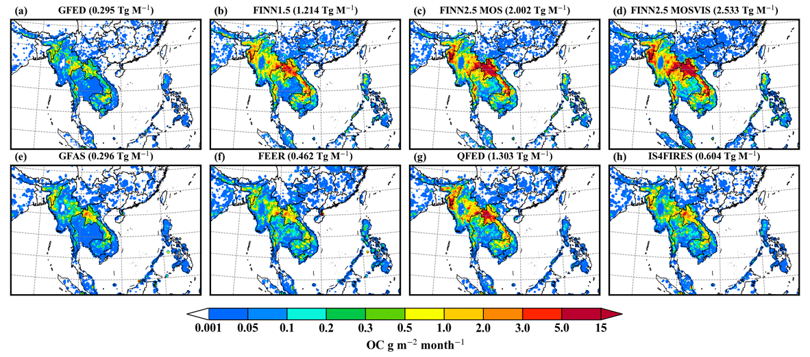
Figure 3 The spatial distribution of eight BB emission inventories of OC in the study region for (a–h) GFED, FINN1.5, FINN2.5 MOS, FINN2.5 MOSVIS, GFAS, FEER, QFED, IS4FIRES, and the total OC emissions in the PSEA region during March 2019.

2.4 Methodology

In order to assess AOD, AAOD, AEC, and DRF using WRF-Chem with different BB inventories, apart from the FINN schemes, other emission inventories are regridded and time-allocated, as shown in Fig. 2. Subsequently, species are supplemented according to the gas-phase chemistry and aerosol scheme (MOZART–MOSAIC) employed by WRF-Chem. It is worth noting that all scenarios utilized fire size and vegetation type proportion data from FINN1.5 to calculate smoke plume rise. The performance of WRF-Chem model simulations against measurements is evaluated using statistical metrics (Wu et al., 2019) including the mean bias (MB), RMSE, correlation coefficient (R), and the index of agreement (IOA) in Table S8. This research further investigated DRF over PSEA during the study period. Zhao et al. (2013) and Lin et al. (2014) were referenced for the treatment of BB aerosol radiative forcing, as shown in the following equations.

$$\begin{array}{}\text{(2)}& \mathrm{DRF}=\left(F_i^{\downarrow }-F_i^{\uparrow }\right)-\left(F_{\text{no-fire}}^{\downarrow }-F_{\text{no-fire}}^{\uparrow }\right),\end{array}$$

where F^↑ and F^↓ indicate the aerosol upward radiation flux and the aerosol downward radiation flux, respectively. i indicates that WRF-chem is added to the different BB emission inventories, and “no-fire” denotes a scenario without BB inventory applied.

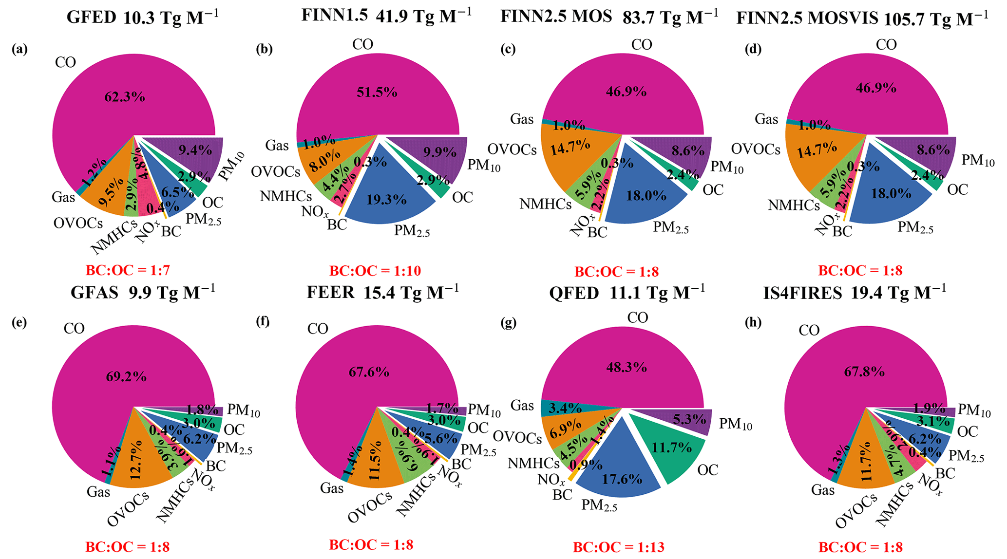
Figure 4 Total emissions and percentage composition of different substances in the eight BB emission inventories (after processing in Fig. 2; i.e., the missing BB data have been supplemented) over PSEA in the WRF-Chem model, which indicates the proportion of BC and OC, where “gas” represents the combination of SO₂ and NH₃. OVOCs contain C, H, and O compounds (ethanol (C₂H₅OH), formaldehyde (CH₂O), acetaldehyde (CH₃CHO), acetone (CH₃COCH₃), methanol (CH₃OH), methyl ethyl ketone (MEK), pentanedial (C₅H₆O₂), acetic acid (CH₃COOH), cresol (C₆H₄(CH₃)(OH)), glyceraldehyde (GLYALD), methylglyoxal (MGLY), glyoxal (GLY), acetol (CH₃COCH₂OH), methacrolein (MACR), methyl vinyl ketone (MVK)). NMHCs refer to organic compounds containing only C and H, besides methane (CH₄), including pentane (C₅H₁₂), butadiene (C₄H₈), ethylene (C₂H₄), ethane (C₂H₆), propane (C₃H₈), propylene (C₃H₆), toluene (C₆H₅(CH₃)), lumped monoterpenes, such as α-pinene (C₁₀H₁₆), and isoprene (C₅H₈). NMHCs and OVOCs combined constitute nearly all of the non-methane volatile organic compounds (NMVOCs) emitted by wildfires. PM_2.5 is the PM_2.5 fraction excluding OC and BC. PM₁₀ is the PM_10–2.5 fraction.

3 Result

3.1 Intercomparison of eight BB inventories

Several studies have utilized OC as a measurable metric to compare variations among multiple BB inventories (Reddington et al., 2016; Carter et al., 2020). This is because OC is a major component in smoke particles from fresh BB, with mass fractions ranging from 37 % to 67 %, depending on the fuel type (Pan et al., 2020). Figure 3 presents the spatial distribution characteristics of OC for the eight BB datasets in the study region, along with the total OC emissions in the PSEA region during March 2019. The highest OC emissions across all datasets are observed in the northern regions of Laos, Cambodia, and Thailand, as well as in eastern and western Myanmar and southern Bangladesh. Lower emissions are observed in the central regions of Myanmar and Thailand, northern Vietnam, and southern regions of China. Similar spatial distribution characteristics of OC emissions in the PSEA region during March have also been reported by Pan et al. (2020) and Reddington et al. (2021). These emissions mainly originate from shrubland, evergreen broadleaf, mixed shrubland/grassland, and dryland cropland, as classified by the WRF-Chem land use data in the PSEA (Fig. S1 in the Supplement). The eight BB emissions, ranked based on their total OC emissions (PSEA) in descending order, are FINN2.5 MOSVIS (2.533 Tg M⁻¹), FINN2.5 MOS (2.002 Tg M⁻¹), QFED (1.303 Tg M⁻¹), FINN1.5 (1.214 Tg M⁻¹), IS4FIRES (0.604 Tg M⁻¹), FEER (0.462 Tg M⁻¹), GFAS (0.296 Tg M⁻¹), and GFED (0.295 Tg M⁻¹). The highest OC emission in the dataset is exhibited by FINN2.5 MOSVIS, which can be attributed to the use of updated burned area data and the inclusion of fire information from VIIRS and which captured a larger number of small-scale fires (Wiedinmyer et al., 2023). The lowest OC emissions are provided by GFED, which may have underestimated DM and agricultural fire EF (OC; EF = 2.3 g kg⁻¹), and GFAS, which only underestimated DM. The overall mean and standard deviation of OC for different BB emission inventories in the PSEA region was 1.09 ± 0.83 Tg M⁻¹, with a coefficient of variation (CV) of 76 % (CV is defined as the ratio of the standard deviation to the mean of all inventories).

Figure 4 illustrates the total emissions of the eight emission inventories in the PSEA region during March 2019 added to the WRF-Chem after processing (Fig. 2). It also presents the percentage composition of CO, OVOCs, NMHCs, NO_X, gas (SO₂ and NH₃), PM_2.5, PM₁₀, BC, and OC. The total BB emissions (aerosol and gas) are ranked as FINN2.5 MOSVIS (105.7 Tg M⁻¹), FINN2.5 MOS (83.7 Tg M⁻¹), FINN1.5 (41.9 Tg M⁻¹), IS4FIRES (19.4 Tg M⁻¹), FEER (15.4 Tg M⁻¹), QFED (11.1 Tg M⁻¹), GFED (10.3 Tg M⁻¹), and GFAS (9.9 Tg M⁻¹). Although the total QFED emissions are low, the aerosol emissions (OC, BC, PM_2.5, and PM₁₀) are not; they are just smaller than the FINN schemes. The PSEA aerosol emissions from FINN2.5 are higher than those predicted for FINN1.5 and approximately twice as high as the latter, consistent with the findings of Wiedinmyer et al. (2023). Among them, the highest and lowest emissions of OC+BC are observed in FINN2.5 MOSVIS (2.82 Tg M⁻¹) and GFAS (0.32 Tg M⁻¹), respectively. Since the FINN schemes employ the EFs from Akagi et al. (2011) and subsequent updates, the proportions of each species are relatively similar. In summary, FINN schemes (v1.5 and 2.5) have relatively high total aerosol emissions compared to the other schemes, and the top-down scenario (GFAS, FEER, QFED, and IS4FIRES) does not have high total emissions, despite being constrained by the AOD. To evaluate the spatiotemporal distribution characteristics of absorbing aerosols from BB emissions, particularly the BC to OC ratio was also displayed in Fig. 4. Except for QFED, which exhibits a lower ratio of approximately 0.08 ($\mathrm{1}/\mathrm{13}$), the ratios for the other BB datasets are greater than or equal to 0.1 ($\mathrm{1}/\mathrm{10}$). Ferrada et al. (2022) found that QFED emission inventories compared to other inventories (GFED4.1s, FINN1.5, and GFAS1.2) increased BC and OC emissions by up to 5 times in different ecological regions. In addition, differences in emission EFs in Southeast Asia may result in a $\mathrm{BC}/\mathrm{OC}$ equal to approximately 0.08.

3.2 Model validation

To assess the AOPs and DRF simulated by the WRF-Chem adding different BB emissions, the stability of the model is verified by comparing the simulated meteorological fields and PM_2.5 concentrations with observations at monitoring stations using the WRF-Chem with the FINN1.5 scheme. The statistical results in Table S6 demonstrate good agreement (IOA ≥ 0.6) between the simulated T2, RH2, and WS10 and the data from 13 stations. However, at some stations, the wind speed RMSE exceeds 2 m s⁻¹, which may be attributed to unresolved topographic features in the surface drag parameterization (Saide et al., 2016). The bias between observations and simulations for RH2 can be partially explained by the influence of different surface and boundary layer parameterizations on the simulated near-surface water vapor fluxes (Chen et al., 2019). During the wildfire period of March 2019, the daily average observed PM_2.5 concentrations of 23 cities at the surface were compared with the model results for the FINN1.5 case in Fig. S2, where the statistical indicators are shown in Table S7. WRF-Chem was able to simulate PM_2.5 concentrations in urban sites located in the BB high-emission region of northern Laos (Mueang Chiang Rai in northern Thailand and Jinghong in China), consistent with to the observed data (R of 0.64 and 0.75, respectively), where the model was able to reproduce the pollution peaks (IOA of 0.74 and 0.82, respectively). In a previous study by Vongruang et al. (2017), the WRF-CMAQ (Community Multiscale Air Quality Model) model was used to simulate PM_2.5 in the PSEA region by incorporating BB emissions (GFAS v1.1 or FINN1.5) and comparing them with observed stations. The average IOA value was 0.51 (with the optimal IOA being 0.69). In this study, all 23 stations had IOA values greater than 0.51 (with over 52 % exceeding 0.69), indicating that the model can consistently reproduce the spatial and temporal distribution characteristics of pollutants in the PSEA region. Although the WRF-Chem model could reasonably capture the spatiotemporal characteristics of PM_2.5 concentrations observed in most cities (IOA > 0.54), the influence of anthropogenic emission inventories and BB vertical transport may lead to biases in some areas (e.g., Hong Kong).

3.3 AOD

3.3.1 Satellites vs. AERONET AOD

The linear regression results between AOD daily averages from different satellite sensors and AERONET data are shown in Fig. S3. Overall, during the wildfire event in the PSEA region, the DB algorithm of VIIRS demonstrated the best skill, as indicated by optimal R² and RMSE values. Su et al. (2022) found that VIIRS DB also exhibited the highest accuracy and stability when analyzing long-term multiple satellite inversions of AOD aerosol datasets in Asia. This is because the VIIRS DB incorporates upgraded surface and aerosol models specifically designed for Asian regions, which have not been applied to the MODIS DB (Sayer et al., 2019). Therefore, to evaluate the representation of AOD in the WRF-Chem experiments for the PSEA wildfires in March 2019, the AOD at 550 nm provided by VIIRS DB (along with AERONET observations) was chosen to determine biases and errors in the conducted experiments.

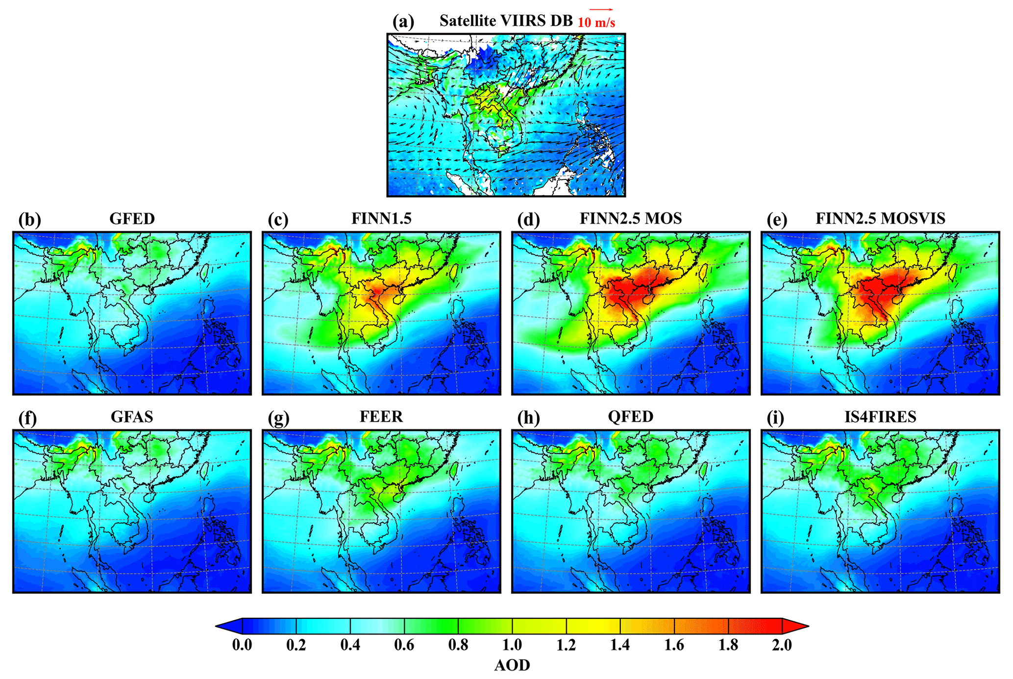
Figure 5 The daily mean AOD retrieved by the VIIRS satellite (a) transiting the PSEA region and the AOD simulated by WRF-Chem with eight corresponding BB emission inventories (b–i: GFED, FINN1.5, FINN2.5 MOS, FINN2.5 MOSVIS, GFAS, FEER, QFED, and IS4FIRES) in the PSEA region during March 2019, with 950 hPa wind (vectors; m s⁻¹) based on ERA5 data from March 2019.

Figure 6 Spatial distribution of MB, RMSE, and R between AOD from the VIIRS satellite vs. AOD simulated by WRF-Chem with eight BB emission inventories (GFED, FINN1.5, FINN2.5 MOS, FINN2.5 MOSVIS, GFAS, FEER, QFED, and IS4FIRES) in PSEA during March 2019, where panels (a-1–8) are the MB for the comparison of the eight BB scenarios, panels (b-1–8) are the RMSE for the comparison of the eight BB scenarios, and panels (c-1–8) are the R for the comparison of the eight BB scenarios.

3.3.2 WRF-Chem vs. VIIRS AOD

To assess the agreement between the simulated AOD from WRF-Chem and the observed AOD, we utilized the extracted data (WRF-Chem) based on VIIRS satellite transit time and compared the daily average values with AERONET observations. Figure 5 illustrates the daily average AOD at 550 nm from the VIIRS and wind (scaled in 10 m s⁻¹) at 900 hPa (Fig. 5a), along with the corresponding AOD from the WRF-Chem simulation over the PSEA region during March 2019, considering different BB scenarios (Fig. 5b-i). The high AOD (HAOD; AOD > 1.0) derived from VIIRS retrievals is primarily concentrated in Laos, Thailand, and Vietnam (15–22.5^∘ N, 97–110^∘ E). Additionally, the Beibu Gulf and coastal cities in southern China also exhibit high-AOD values (AOD > 0.6), which may be attributed to the long-range BB transport of tropical westerly and southwesterly winds depicted in Fig. 5a. The FINN (v1.5 and 2.5), FEER, QFED, and IS4FIRES schemes demonstrate the ability to reproduce high-aerosol concentrations in areas with elevated AOD values, as observed by VIIRS satellites. These simulations align with the spatial distribution of monthly mean AOD during the wildfire period in the PSEA simulations conducted by Dong and Fu (2015a). However, the GFED and GFAS schemes fail to capture the high-AOD areas in the PSEA region, likely due to the BB low-emission inventories of the input model (Pan et al., 2020).

Table 2 Evaluation of WRF-Chem AOD and AAOD vs. satellites in the HAOD (15–22.5^∘ N, 97–110^∘ E) region during March 2019.

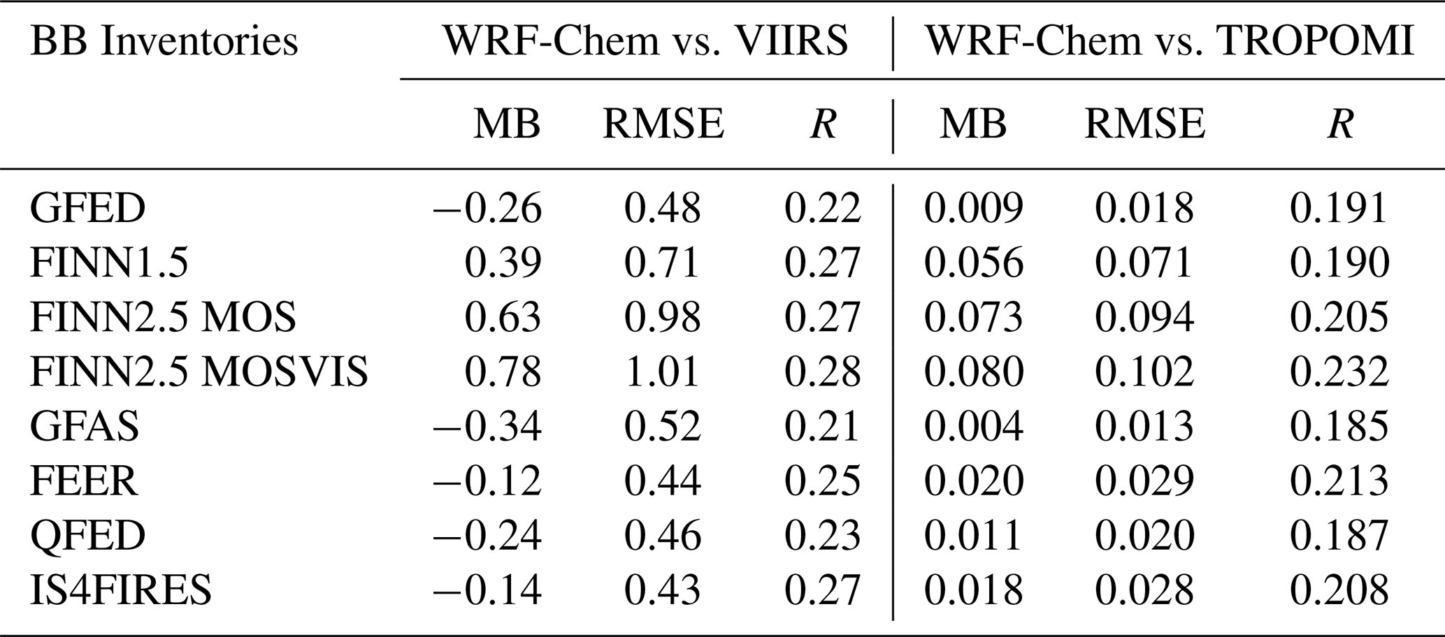
Figure 6a-1–8 displays the estimated MB between the model, with eight BB scenarios and VIIRS daily mean AOD. The FINN schemes (v1.5 and 2.5) noticeably overestimate AOD in the HAOD region, while the GFED, GFAS, FEER, and IS4FIRES schemes underestimate AOD. Moreover, the FINN schemes also exhibit AOD overestimation in the Beibu Gulf, South China Sea, Bay of Bengal, and Andaman Sea. As the FINN schemes have the largest aerosol emissions compared to other BB emissions (Fig. 4), it may lead to an overestimation of AOD in the HAOD region. All schemes exhibit varying degrees of overestimation for a significant portion of southern China. Table 2 provides statistics on the MB of AOD between satellite-retrieved and WRF-Chem AOD in the HAOD region. The AOD simulated by FINN schemes is significantly overestimated, whereas the rest of the schemes exhibit underestimation. Although FEER (−0.12) and IS4FIRE (−0.14) underestimate the simulated AOD, their performance is considerably better than other BB emission inventories. As highlighted by Palacios-Pena et al. (2017) and Crippa et al. (2019), the MB between simulated and observed AOD can be attributed to estimation errors in BB uncertainty and aerosol dry mass and are specifically related to the certain mass of small particles or too much moisture associated with the aerosol. The RMSE estimation (Fig. 6b-1–8) reveals noticeable uncertainty in the FINN schemes when compared to other schemes in the HAOD and southern China, while the performance of the remaining schemes in simulating AOD in Laos and northern Thailand is unsatisfactory. The RMSE statistics in Table 2 show that the AOD simulated by the FINN2.5 schemes (MOS and MOSVIS) has greater uncertainty in the HAOD region compared to FINN1.5, and the RMSE of the other schemes is generally comparable. Figure 6c-1–8 depicts the temporal R between simulated AOD and observations, with high values of R (> 0.6) concentrated in Laos and northern Thailand, Myanmar, the Bay of Bengal, the Andaman Sea, and the South China Sea. The FINN2.5 MOSVIS scheme exhibits the highest R compared to other schemes in the HAOD region (Table 2), potentially due to the updated acquisition time (local time) and increased VIIRS data, leading to improved R with the observed data.

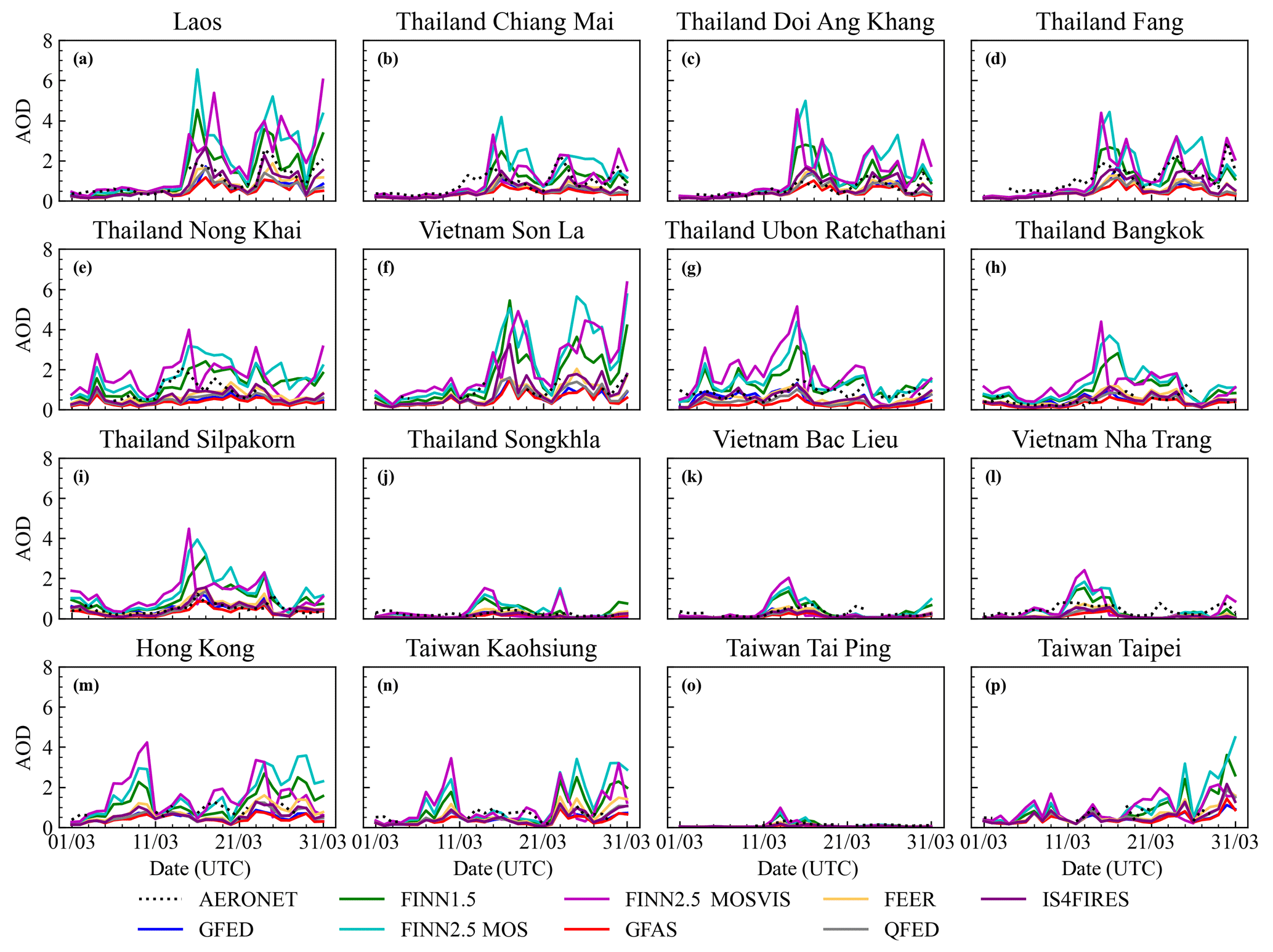
Figure 7 Time series of daily average AOD (550 nm) simulated by WRF-Chem including eight BB emissions in March 2019 compared to 16 AERONET sites (a–p). These stations are divided into three categories, where the first category of stations is located within the HAOD range of satellite inversion (15–22.5^∘ N, 97–110^∘ E; a–g). The second type consists of observational sites located in adjacent high-AOD regions (AHAOD; h–l). The third type encompasses observational sites situated within the downwind areas (DAs; m–p). The legend line characterizes different BB simulation scenarios.

Table 3 WRF-Chem AOD at 550 nm vs. AERONET in HAOD, AHAOD, and DA during the wildfire period, where HAOD includes Laos, Chiang Mai, Doi Ang Khang, Fang, Nong Khai, Son La, and Ubon Ratchathani stations.

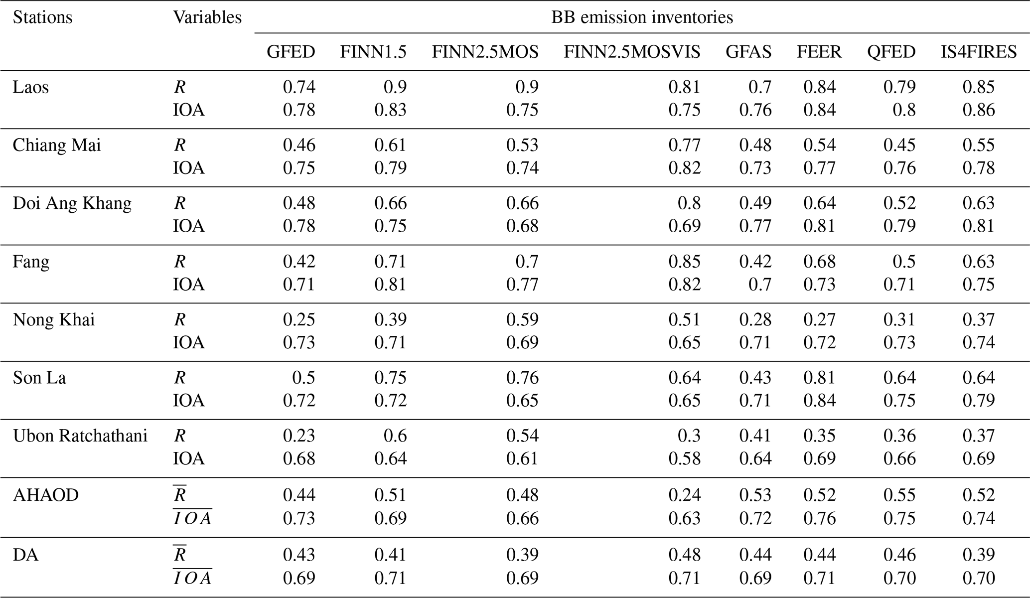
Note: AHAOD and DA only contain the corresponding site mean R and IOA.

3.3.3 WRF-Chem vs. AERONET AOD

Figure 7 illustrates the time series of AOD at 550 nm, measured at the 16 AERONET sites marked in Fig. 1, in comparison to simulated AOD from WRF-Chem with different BB emissions. These 16 sites are categorized into three major classes, namely the satellite inversion of HAOD regions (15–22.5^∘ N, 97–110^∘ E; Fig. 7a–g), the adjacent HAOD area (AHAOD; Fig. 7h–l), and the downwind area (DA; Fig. 7m–p), allowing for further analysis of AOD variations during wildfire events. In the HAOD stations (Laos, Chiang Mai, Fang, Nong Khai, Son La, and Ubon Ratchathani), high aerosol loading was captured by all schemes and AERONET sites on 15, 23, and 30 March, respectively. Among the sites, the Laos station performed the best in terms of simulated and observed AOD mean R and IOA for all BB scenarios, with R and IOA values of 0.82 and 0.80, respectively (Table 3). To compare the performance of the multi-BB emission scenario model for the AOD simulation, a Taylor diagram was constructed (Fig. 8). The Taylor diagram demonstrates that, in the HAOD regions, the FINN schemes (v1.5 and 2.5) exhibit a higher overall R when compared to other schemes when simulating AOD against observations. Furthermore, the FINN2.5 schemes show a slightly better correlation than FINN1.5. Among the eight schemes, the IS4FIRES and FINN1.5 schemes simulated AOD performed better in terms of consistency and deviation from the observed comparison in the HAOD region (Fig. 8a). In the AHAOD stations, peaks of AOD simulated by WRF-Chem were also found on three dates (15, 23, and 30 March), but these peaks were lower than the HAOD in Fig. 7. Despite the FINN2.5 MOSVIS scheme showing the best correlation between simulated AOD and observations in the HAOD regions compared to other schemes, its performance in AHAOD regions was unsatisfactory (Table 3). Poorly performing stations in the AHAOD regions included Bangkok, Silpakorn, and Songkhla, which are located between 0^∘ and 22.5^∘ N (Fig. 7). This discrepancy may be attributed to the assumptions made by the FINN2.5 MOSVIS scheme for fire detection in the equatorial region to achieve daily global coverage (Wiedinmyer et al., 2023) and the overestimation of AOD values by WRF-Chem, which can be explained by the presence of excess aerosol dry mass (Chapman et al., 2009). In the DA regions, such as Hong Kong and Taiwan, high concentrations of aerosols were simulated and observed after 23 March in Fig. 7. Previously, others studied the same event using models and ground measurements and reported a contribution of BB of about 56 % to local AOD and 26 %–62 % to DA.

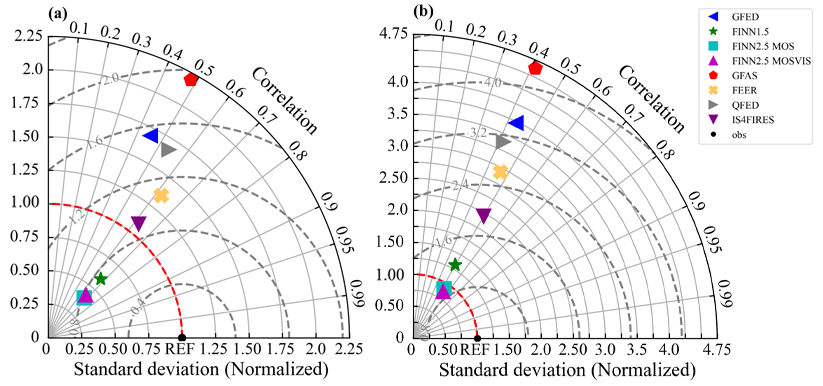
Figure 8 Taylor diagrams of (a) AERONET vs. WRF-Chem AOD at 550 nm and (b) AERONET vs. WRF-Chem AAOD at 500 nm in the HAOD region (15–22.5^∘ N, 97–110^∘ E) during the wildfire period.

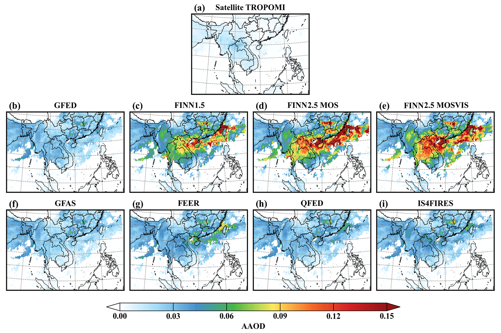
Figure 9 Spatial distribution of AAOD between Sentinel-5 TROPOMI satellite (a) vs. AAOD simulated by WRF-Chem with eight BB emission inventories (b–i) during wildfire period in PSEA.

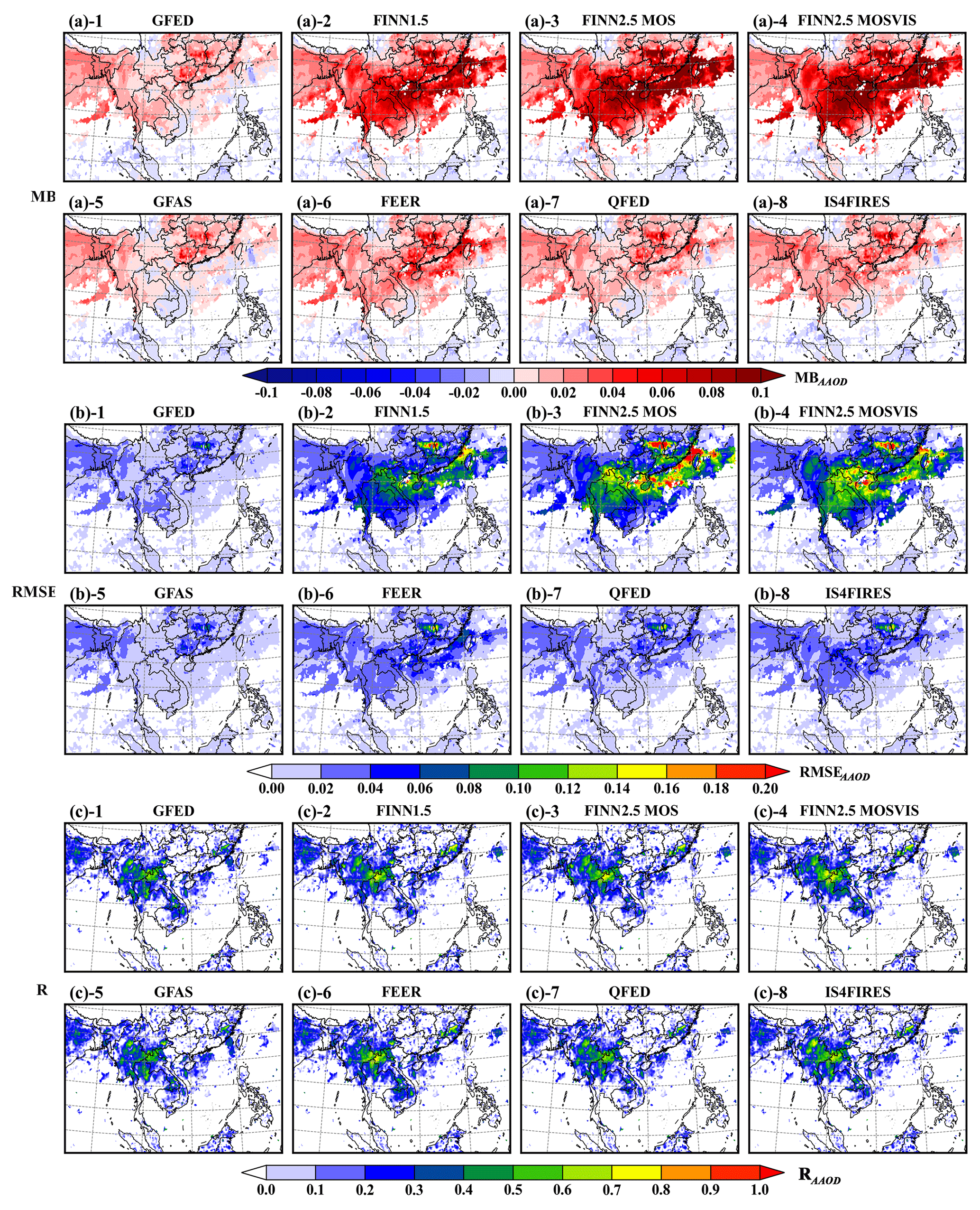
Figure 10 Spatial distribution of MB, RMSE, and R between AAOD from TROPOMI satellite vs. AAOD simulated by WRF-Chem with eight BB emission inventories (GFED, FINN1.5, FINN2.5 MOS, FINN2.5 MOSVIS, GFAS, FEER, QFED, and IS4FIRES) in PSEA during March 2019, where panels (a-1–8) are the MB for the comparison of the eight BB scenarios, panels (b-1–8) are the RMSE for the comparison of the eight BB scenarios, and panels (c-1–8) are the R for the comparison of the eight BB scenarios.

3.4 AAOD

3.4.1 WRF-Chem vs. TROPOMI AAOD

Wildfire releases significant amounts of absorbing aerosols such as OC and BC, which can absorb solar radiation and increase the radiation absorption capacity of the atmosphere, thereby affecting the Earth's radiation balance. Therefore, it is crucial to evaluate the model's ability to simulate absorbing aerosols using AAOD results obtained from satellite observations. To reduce the discrepancies caused by missing data in the inversion of different observations, the WRF-Chem simulations are matched with the observed data. Figure 9 shows the spatial distribution of daily mean AAOD at 500 nm retrieved by TROPOMI (Fig. 9a) and simulated by WRF-Chem with eight BB emissions (Fig. 9b–j) during March 2019 in the PSEA region. The high AAOD (AAOD > 0.03) from TROPOMI is mainly concentrated in northern Laos, northern Vietnam, northern Thailand, and eastern Vietnam, which is similar to the spatial distribution characteristics of HAOD provided by VIIRS. Kang et al. (2017) also found similar AAOD distribution patterns when studying the spatial and temporal characteristics of absorbing aerosols in Southeast Asia from 2005 to 2016. The WRF-Chem simulations with different BB emissions exhibit high-AAOD values not only in the aforementioned regions but also in southern China and the South China Sea (Fig. 9). Figure 10 shows the spatial distribution characteristics of MB (Fig. 10a), RMSE (Fig. 10b), and R (Fig. 10c) for the comparison of TROPOMI-inverted AAOD with WRF-Chem-simulated AAOD using different BB scenarios. The FINN, FEER, and IS4FIRES schemes all overestimate AAOD in the HAOD region (15–22.5^∘ N, 97–110^∘ E), when compared to the TROPOMI inversion, with FINN2.5 showing the most significant overestimation (Fig. 10a-1–8). Table 2 further confirms these overestimations with statistics of 0.056, 0.073, 0.08, 0.02, and 0.018, respectively. The overestimation may arise from underestimating AAOD in TROPOMI, as well as overestimating absorbing aerosols in the BB inventory and uncertainties in the representation of absorbing aerosols by WRF-Chem, including aerosol size distribution, chemical composition, aging processes, vertical and horizontal transport (including injection heights for fire emissions), and errors in dry/wet removal from the atmosphere. Figure 10b-1–8 and Table 2 demonstrate that the FINN schemes exhibit greater uncertainties in simulating AAOD in the HAOD region compared to other schemes. Comparing the R between satellite-retrieved AAOD and simulated AAOD, values of R > 0.6 are primarily concentrated in northern Laos, northern Thailand, and Myanmar. Particularly, the FINN2.5 MOSVIS scheme, due to the incorporation of improved local time and inclusion of small fires from VIIRS, exhibits the best correlation with the simulated AAOD relative to satellite retrievals (Table 2).

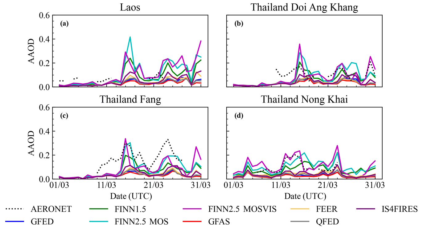
Figure 11 Comparisons of time series between daily mean AAOD at 500 nm measurements provided by four AERONET sites within the HAOD range and AAOD simulated by the nearest corresponding AERONET site using WRF-Chem and adding different BB inventories, where the satellite inversions of both AOD > 1 and AAOD > 0.03 (range 15–22.5^∘ N, 97–110^∘ E) are called HAOD. The legend line is the same as in Fig. 7.

3.4.2 WRF-Chem vs. AERONET AAOD

To reduce the uncertainty caused by missing AERONET data, quality control has been applied to the AERONET site data (samples > 10 d). In the HAOD region within the range of 15–22.5^∘ N, 97–110^∘ E, where both the satellite-retrieved AOD and AAOD exceed the thresholds of 1 and 0.03 (BB high-emission area), respectively. Figure 11 presents a comparison of the time series between AAOD measurements from four AERONET sites within the HAOD region and AAOD simulated by the nearest corresponding AERONET site using WRF-Chem with different BB inventories. Similar to peaks of AOD, AAOD from the Doi Ang Khang site also exhibits peaks on 15, 23, and 30 March. Although most schemes can capture the high-AAOD loading, the performances of the GFED, GFAS, and QFED schemes are unsatisfactory (Table S9). This could be attributed to lower concentrations of absorbing aerosols or inaccurate spatial distribution in the BB emission inventories (Reddington et al., 2016). The Fang site shows the best mean R and IOA among the eight BB scenarios simulating AAOD compared with AERONET, with R and IOA values of 0.69 (Table S9). The Taylor diagram indicates that the FINN schemes perform better than others in representing AAOD in Fig. 8b, which may be the FINN schemes for unique calculating the biomass burned area and EFs that are more suitable for the HAOD region (Wiedinmyer et al., 2011, 2023). When comparing simulated AAOD with observations for the FINN2.5 MOSVIS scheme, both the R and IOA perform better than other schemes at all sites. The improved performance of the FINN2.5 MOSVIS scheme in simulating AAOD during wildfires in the PSEA region can be attributed to the following two factors: the inclusion of smaller fires using VIIRS 375 m fire detection data and updated information on time and burned area.

3.5 AEC

Although AOD and AAOD provide useful information about atmospheric aerosol loading, there is limited information available regarding the vertical distribution of aerosols. Palacios-Peña et al. (2018) found that the uncertainty in the vertical distribution of aerosols during wildfires in Europe affects AOPs. The CALIPSO, with its unique capability to actively retrieve vertical aerosol spatial distribution, offers an opportunity to assess the simulation of aerosol vertical optical properties by WRF-Chem during wildfire events. Figure 12 displays the aerosol vertical extinction profiles at 532 nm retrieved by CALIPSO in the HAOD region during March 2019, along with the aerosol extinction profiles (550 nm) simulated by various BB schemes, where model data are matched with CALIPSO overpass times. AEC retrieval by CALIPSO is greater than 0.2 within the range of 0.5 km to 4 km above ground level, possibly due to the uplifted aerosols from wildfires. WRF-Chem utilizes the smoke plume rise model, with the upper and lower limits of heat flux determined for each land type, to calculate the minimum and maximum plume heights, and the emitted pollutants are distributed across each vertical layer within the injection height (Grell et al., 2011). From 0.5 to 4 km, the trends of the AEC changes in the eight BB schemes are consistent with CALIPSO, indicating that the employed smoke plume rise model in WRF-Chem can reproduce the minimum and maximum plume heights. However, all the FINN schemes overestimate AEC compared to CALIPSO from 0.5 to 4 km, while the other schemes underestimate it. The aerosol concentration in the BB emission inventories may play a decisive role, leading to differences in the AEC (Reddington et al., 2019). Figure S4 illustrates the frequency distribution of six aerosol types at an altitude of 8 km over the PSEA region in March 2019. Within the higher altitudes of 5–7 km, the presence of dust, polluted dust, and smoke aerosols is evident, with the dust aerosols originating from the upper-level westerlies in the Indian subcontinent region. Within this altitude range, the simulated AEC gradually approaches zero with increasing altitude. However, the AEC retrieved by CALIPSO exhibits three peaks, which may be attributed to uncertainties in the calculation model for BB injection heights and the influence of external dust transport.

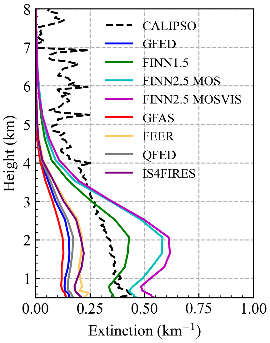
Figure 12 Vertical distributions of monthly mean aerosol extinction (550 nm) from WRF-Chem with different BB inventories and the corresponding CALIPSO retrieval (532 nm) in HAOD (15–22.5^∘ N, 97–110^∘ E). The dotted black line indicates CALIPSO, and the remaining lines are the same as in Fig. 7.

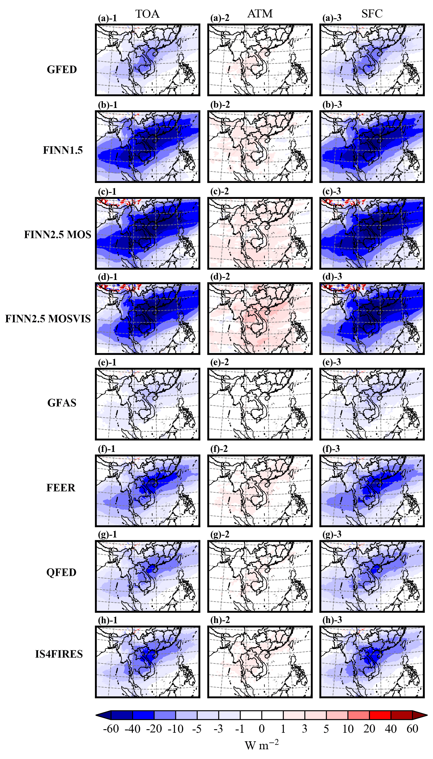
Figure 13 The average difference in clear-sky SW radiation fluxes (daytime) simulated with and without BB emissions (GFED, FINN1.5, FINN2.5 MOS, FINN2.5 MOSVIS, GFAS, FEER, QFED, IS4FIRES) over the PSEA in March 2019 at the top of the atmosphere (TOA), ground surface (SFC), and in the atmosphere (ATM), where panels (a–h) represent eight emission inventories.

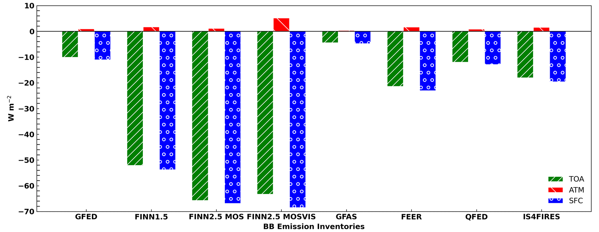
Figure 14 The average difference in clear-sky SW radiation fluxes (daytime) simulated with and without BB emissions in the HAOD (15–22.5^∘ N, 97–110^∘ E) region during March 2019.

3.6 DRF

Considering the significant impact of BB aerosols on radiation, this study investigates the radiative perturbation of SW radiation caused by BB aerosols under clear-sky conditions at the top of the atmosphere (TOA), surface (SFC), and in the atmosphere (ATM). The focus is on the DRF of BB aerosols during the daytime, as Ge et al. (2014) found that local convergence in the smoke source region caused by smoke during the daytime transmits more smoke particles on the above surface. Figure 13 illustrates the spatial distribution of the daytime average SW radiative perturbation caused by BB aerosols during March 2019 in the PSEA region at the TOA, ATM, and SFC. It is evident that BB aerosol DRF exists not only in the PSEA region but also in other regions such as southern China, Hong Kong, and Taiwan. The spatial distribution of SW radiative perturbation by BB aerosols aligns with the simulated distribution of AOD, with the highest values observed in the HAOD region (15–22.5^∘ N, 97–110^∘ E). Lin et al. (2014) have confirmed that BB aerosols, mainly BC and OC, play significant roles in the radiative budget. On one hand, the solar absorption by BC in the atmosphere increases the rate of radiative heating, leading to a significant decrease in solar radiation reaching the surface. On the other hand, OC enhances the reflected solar radiation at the TOA, resulting in a cooling effect due to reduced incidental solar radiation in the atmosphere and surface. The SW radiative perturbation of BB in TOA is negative, with a cooling effect in the model domain for eight scenarios, except for areas with high surface albedo such as Himalayan glaciers. Figure 14 shows that during the wildfire period in the HAOD region, the eight schemes exhibit DRF of −30.89 ± 23.6 W m⁻² at TOA. The SW radiative perturbation of BB aerosol at TOA depends largely on the SW absorption rate of BB aerosol. The FINN schemes (v1.5 and 2.5) exhibit a significantly stronger cooling effect compared to other schemes, possibly due to higher BC concentrations in BB emissions compared to other inventories. At the ATM, the absorption by BB aerosols leads to a positive radiative forcing, causing atmospheric warming, particularly in the HAOD region. In the HAOD region, the eight schemes exhibit a BB aerosol SW DRF of 1.70 ± 1.40 W m⁻² in the ATM (Fig. 14). WRF-Chem can simulate the heating effect of BB aerosols in the ATM regardless of the $\mathrm{BC}/\mathrm{OC}$ ratio used in the emission inventory (1:8, 1:9, or 1:13). At the SFC, the cooling effect is due to the scattering of non-absorbing atmospheric aerosols and absorbing aerosols that increase the radiative heating rate, resulting in a significant reduction in the solar radiation reaching the surface. The eight schemes simulate the DRF of −32.60 ± 24.50 W m⁻² at SFC in the daytime, with FINN2.5 MOSVIS reaching a maximum of approximately 70 W m⁻² (Fig. 10), which is comparable to the level of the PSEA region studied previously by Lin et al. (2014) and Ge et al. (2014).

4 Discussion

Biases in the simulated AOPs (AOD, AAOD, and AEC) over tropical BB have been attributed to a variety of factors (Reddington et al., 2016), including (1) uncertainties in BB emission fluxes and (2) errors in modeling the atmospheric distribution and properties of BB aerosols. These deviations in optical properties further affect the DRF, leading to uncertainties in the assessment of climate change.

4.1 BB emission fluxes

Uncertainties associated with the derivation of emission fluxes arise from errors in the satellite detection of active fire or burned areas (e.g., cloud and smoke obscuration of the surface, satellite spatial resolution and detection limitations, and satellite exceedance times), as well as uncertainties in EF and fuel consumption estimates (Carter et al., 2020; Wiedinmyer et al., 2023). Eight BB inventories were inverted from MODIS data, but there were significant gaps between the bandwidths of MODIS in the equatorial region, as well as difficulties in detecting fires located under thick clouds, and a reduction in fire detection sensitivity at the scan edge sensitivity, leading to an underestimation of total regional BB emissions (Wang et al., 2018). In this paper, the FINN2.5 dataset (BB emission fluxes and AOPs) is consistently higher than the other datasets, with FINN2.5 MOSVIS being the highest overall. FINN2.5 includes improved burned-area calculations, uses year-specific land cover and vegetation datasets, updates fuel loads and EFs, and can use multiple fire detection satellite inputs (e.g., MODIS and VIIRS), which may account for the improved BB emission fluxes. In the PSEA region, during wildfire events, the BB emissions from FINNv2.5 are consistently higher than the emissions provided by FINNv1.5, approximately twice as much as the latter, even when considering only MODIS fire detections. The increase in emissions is primarily attributed to the new treatment of burned areas (Wiedinmyer et al., 2023). Despite updates to input data, parameters, and processing methods, the FINN2.5 scheme tends to overestimate AOPs compared to observations. This overestimation may arise from inaccurate ecosystem identification (e.g., tropical forests instead of shrublands or areas with fewer trees) and fuel load allocation (Pan et al., 2020). Furthermore, in tropical regions, the FINN scheme employs the smoothing of fire detection to mitigate the impact of clouds, which could lead to an overestimate of BB emissions (Wiedinmyer et al., 2011, 2023). QFED provides relatively higher OC concentrations but lower total BB emissions, and the primary driving factors behind these differences are the assumed fuel types and related EFs. Therefore, it is inappropriate to consider OC as the sole criterion for evaluating BB emission fluxes when comparing multiple BB emission inventories. Although the aerosol concentrations provided by QFED are larger than those of IS4FIRES and FEER, the simulated AOPs and DRF of this scheme are lower than those of the latter, which may be due to the influence of secondary pollutant emission precursors (NO₂, NH₃, etc.). Previous studies have often used an expansion of aerosols (BC + OC) in the BB emission inventories by a factor of 3–6 to assess the AOPs (Reddington et al., 2016; Marlier et al., 2013), and the simulation results from the QFED scheme above reveal that there may be significant uncertainties in this expanded aerosol (BC+OC) approach. Although GFED4.1s improves the detection of small fires, the agricultural EF = 2.3 g kg⁻¹ is lower than in other emission inventories, which could result in an underestimation of AOPs simulated by WRF-Chem with the GFED scheme. Yin (2020) found that BB in the PSEA region from 2001 to 2018 was predominantly driven by agro-residue burning and shrubland fires, while the GFED4.1s underestimation of DM for both fires and the mismatch in vegetation types may have contributed to the underestimation of BB emission fluxes (Reddington et al., 2016). In general, FRP-based estimation methods, such as GFAS, FEER, QFED, and IS4FIRES, allow for a more direct estimation of fuel consumption from fire-release energy without the uncertainty associated with the estimation. However, in the PSEA region, when the FRP from MODIS inversion is observed at a nominal spatial resolution of 1 km at its nadir, it risks missing a large number of smaller fires, as well as missing fires that are obscured by clouds (Dong and Fu, 2015a), which may lead to an underestimation of the simulated AOPs. Furthermore, the representation of aerosols in the BB emission inventories is insufficient, including chemical components, the size distribution of aerosols, aging processes, hygroscopic growth, vertical and horizontal transport (including the injection height of fire emissions), and the oxidation state (Reddington et al., 2016), which can all lead to modeling biases in AOPs. Importantly, these attributes also have an impact on aerosols in cloud and radiative forcing.

4.2 Modeling uncertainty and calculation bias

There may be uncertainties in the gas-phase chemistry and aerosol scheme selected to characterize BB aerosols in the model (e.g., growth of aerosol hygroscopicity, scale distributions, aging processes, and wet and dry deposition), which may lead to inaccurate simulation results (Palacios-Peña et al., 2018; Reddington et al., 2016). Sensitivity experiments using the global aerosol model reveal that calculations of hygroscopicity growth are most sensitive in simulating AOD (Reddington et al., 2016). The contribution of SOA formed through the oxidation of VOCs in BB plumes is also a significant source of uncertainty (Jathar et al., 2014). In this study, we employed the meteorological chemistry and aerosol scheme, namely MOZART-MOSAIC_4bin_aqueous, which includes aqueous-phase chemistry and SOA, but this mechanism may lead to an overestimation/underestimation of AOPs in the model. The smoke plume rise model developed by Freitas et al. (2010) was used to vertically represent smoke plumes. Although all schemes capture the vertical profiles of BB aerosol extinction from 0.5 to 4 km altitude, some deviations still exist. Previous research has indicated that assuming all fire emissions injected at the top of the plume could be a worse assumption than prescribing surface-based emissions, which may lead to deviations in simulated AOPs (Mallia et al., 2018). The AEC is not characterized in all BB scenario simulations for 4–8 km, which may also lead to an underestimation of AOD or AAOD, and this high-level perturbation of AEC may come from the influence of external dust aerosols; so, the model emission inventory should consider the effect of dust emissions. Despite the influence of sea salt aerosols in the near-surface region of PSEA (Fig. S4), the contribution of sea salt aerosol to AOD is notably small, approximately 2 % (Zeng et al., 2023). Additionally, Dong and Fu (2015b) observed that the model, during the period from 2006 to 2010, accurately simulated BB AOD without incorporating sea salt emissions over the PSEA region. Consequently, our model does not consider sea salt emission inventories. Other studies have also found that uncertainties in anthropogenic emission inventories can also lead to simulation errors in AOPs and DRF during wildfires in the PSEA region (Dong and Fu, 2015b). Although we used the latest version of the EDGAR 2015 data, there may be some underestimation of such emission inventories due to a large number of incoming factories in the PSEA region (Yang, 2016). Additionally, the inclusion of ARI and aerosol–cloud interactions (ACIs) in the WRF-Chem model has been found to effectively improve the simulation of AOPs in European wildfire simulations (Palacios-Peña et al., 2019), whereas this study only incorporates ARI. ACIs are concerned with aerosols altering the albedo and lifetime of clouds (Baró et al., 2016). Failure to account for ACIs may result in models that do not accurately simulate cloud droplet numbers and sizes, lifetimes, and radiative balances, with implications for climate and atmospheric AOPs (Gao et al., 2022). There is some uncertainty in the AOD from the VIIRS satellite inversion and in the SSA and AAOD from the TROPOMI inversion due to cloud cover effects in the PSEA region, which may also lead to biased assessments. In addition, the closest proximity method used in the gridding process of BB emission inventories can also lead to some calculation errors.

5 Summary and conclusion

This study conducted sensitivity analyses to simulate AOPs and DRF in the PSEA region using eight commonly global BB emission inventories (GFED, FINN1.5, FINN2.5 MOS, FINN2.5 MOSVIS, GFAS, FEER, QFED, and IS4FIRES) and the WRF-Chem model. The main findings can be summarized below.

Regarding BB emissions in the PSEA region, high OC emissions in all datasets (BB) are mainly concentrated in the northern parts of Laos, Cambodia, Thailand, and in eastern Myanmar, with a difference in emissions of about a factor of 9 (0.295–2.533 Tg M⁻¹), an overall mean and standard deviation of 1.09 ± 0.83 Tg M⁻¹, and a CV of 76 %, respectively. Those high BB emissions are primarily from savanna and agricultural fires. OC emissions in GFED and GFAS are significantly lower than in the other inventories. This is attributed to lower DM and agricultural fire EFs in GFED, while DM is underestimated in GFAS. The OC in FINN2.5 MOSVIS is about twice as high as that in FINN1.5, which is explained by the difference in DM rather than EFs. Total aerosol emissions are relatively high in the FINN scenarios (v1.5 and 2.5) compared to the other scenarios. Although the top-down' emission inventories (GFAS, FEER, QFED, and IS4FIRES) are constrained by the AOD from MODIS, the total aerosol emission flux is still insufficient.

The AOD from VIIRS (DB algorithm) demonstrates the best ability to retrieve the AOD compared to AERONET data. An evaluation of the AOPs in the PSEA region during March 2019 reveals different performances between observations (VIIRS, TROPOMI, and AERONET) and BB emission inventories. When comparing the AOD simulated by WRF-Chem with the observed AOD from VIIRS, the FINN1.5, FEER, QFED, and IS4FIRES schemes show a better ability to reproduce high-aerosol concentrations in the HAOD region, while the GFED and GFAS schemes show limitations in characterizing these regions. The FINN (v1.5 and 2.5) schemes tend to overestimate AOD in the region, while other schemes underestimate AOD. The comparison with AERONET data further highlights the performance of different BB emission scenarios, with the FINN1.5 and IS4FIRES scenarios generally showing better agreement with observations. For an AAOD comparison, it was found that the WRF-Chem simulations with different BB scenarios were less capable of simulating AAOD than AOD. The unsatisfactory performance of the GFED, GFAS, and QFED schemes may be due to low concentrations of absorbing aerosols or inaccuracies in the spatial distribution of BB emissions. Among the evaluated BB scenarios, the FINN1.5 schemes generally performed better in representing AAOD. In particular, the FINN2.5 MOSVIS scheme, due to the incorporation of improved local time and inclusion of small fires from VIIRS, exhibits the best R with the simulated AOD and AAOD relative to observations. CALIPSO observations versus AEC simulated by WRF-Chem suggest that the smoke plume rise model can reproduce the minimum and maximum smoke plume heights of wildfire aerosols. However, the FINN (v1.5 and 2.5) schemes tend to overestimate the AEC compared to CALIPSO, while the other scenarios underestimate it. Regarding the DRF, the spatial distribution of the SW radiative disturbances due to BB aerosols closely follows the pattern of the AOD. The FINN (v1.5 and 2.5) schemes exhibit a stronger cooling effect at TOA, which may be due to the higher BC concentration in its emissions. In the HAOD region, BB aerosols exhibited a daytime SW radiative forcing of −32.60 ± 24.50 W m⁻² at the SFC, positive forcing (1.70 ± 1.40 W m⁻²) in the ATM, and negative forcing (−30.89 ± 23.6 W m⁻²) at the TOA. Overall, the FINN scenarios (especially FINN2.5) result in an overestimation of the AOPs in the PSEA region due to an overestimation of DM rather than EFs, which in turn may lead to an overestimation of the DRF. Although the FINN2.5 MOSVIS scenario presents an overestimation of AOPs, the R is the best. Although the top-down emission inventory (GFAS, FEER, QFED, and IS4FIRES) is constrained by the AOD from MODIS, the total aerosol emission flux is still insufficient, which leads to an underestimation of the AOPs modeled by WRF-Chem in the PSEA region. In addition, uncertainties in anthropogenic emissions, dust emissions, and vertical distribution of aerosol concentrations may be attributed to differences from simulations versus observations during the wildfire period in the PSEA region.

Additional evaluations of satellite-based fire emission inventories, particularly in large BB source regions (PSEA), would contribute to a deeper understanding of the uncertainties associated with fire emissions. In the PSEA region, greater attention should be given to the impacts of small fires, cloud cover, different ecosystem types, and EFs during various burning stages and ecosystem types on the inversion of BB emission inventories. To further explore the subsequent effects of BB emissions (e.g., AOPs and radiative forcing), additional investigation of fire aerosol aging and treatment uncertainties (e.g., injection height, mixing state, and SOA formation) is needed. Our study demonstrates that the uncertainty in BB emission inventories is an important factor influencing the WRF-Chem simulation of air quality and climate during wildfires, although the limitations of the model itself should not be overlooked. In the future, we will conduct additional sensitivity experiments and utilize more observational data to further validate the aforementioned uncertainties.

Appendix A: Abbreviations and acronyms

AAOD	Absorbing aerosol optical depth
AEC	Aerosol extinction coefficient
AHAOD	Adjacent HAOD area
AOD	Aerosol optical depth
AOPs	Aerosol optical properties
ATM	In the atmosphere
BB	Biomass burning
BC	Black carbon
CALIPSO	Cloud-Aerosol Lidar and InfraredPathfinder Satellite Observations
CAM-chem	Community Atmosphere Model withChemistry
DA	Downwind area
DRF	Direct radiative forcing
DM	Dry matter
EDGAR	Emissions Database for GlobalAtmospheric Research
EFs	Emission factors
FEER	Fire Energetics and Emissions Research
FINN	Fire INventory from NCAR
FRP	Fire radiative power
GEOS-Chem	Goddard Earth Observing Systemwith Chemistry
GFAS	Global Fire Assimilation System
GFED	Global Fire Emissions Database
HAOD	High AOD
IS4FIRES	Integrated Monitoring and ModellingSystem for Wildland FIRES project
LW	Longwave
MEGAN	Model of Emissions of Gases andAerosols from Nature
MODIS	Moderate Resolution ImagingSpectroradiometer
MOSAIC	Model for Simulating AerosolInteractions and Chemistry
MOZART	Model for Ozone and Relatedchemical Tracers
NMHCs	Non-methane hydrocarbons
NMVOCs	Non-methane volatile organiccompounds
OC	Organic carbon
OVOCs	Oxygenated volatile organiccompounds
PSEA	Peninsular Southeast Asia
PM	Particulate matter
QFED	Quick Fire Emissions Dataset
RH2	2 m relative humidity
SFC	At the surface

SOA	Secondary organic aerosol
SSA	Single scattering albedo
SW	Shortwave
T2	2 m temperature
TOA	The top of the atmosphere
TPM	Total particle matter
VIIRS	Visible Infrared Imaging RadiometerSuite
WS10	10 m wind speed