Individual coal mine methane emissions constrained by eddy covariance measurements: low bias and missing sources

China's Shanxi Province accounts for 12 % of global coal output and therefore is responsible for a very large fraction of the total global methane (CH₄) emissions, as well as being a large source of uncertainty due to the lack of in situ and field measurements. This work introduces the first comprehensive attempt to compute the coal mine methane (CMM) emissions throughout Shanxi, using a mixture of bottom-up and top-down approaches. First, public and private data from 636 individual coal mines in Shanxi Province were analyzed following the IPCC Tier 2 approach, using three to five sets of observed emission factors and rank information based on methods issued by the National Coal Mine Safety Administration and the National Energy Administration, to compile a range of bottom-up CMM on a mine-by-mine basis. An eddy covariance tower is set up near the output flue of a well-characterized high-rank coal mine in Changzhi and used to produce an average observed CH₄ flux over two 2-month-long periods (Winter 2021 and Autumn 2022). The observed half-hourly CH₄ flux variability is found to be roughly stable over the entire observed time and is subsequently used to produce a set of scaling factors (ratio correction) to update the preliminary bottom-up coal mine methane emissions to account for both bias and high-frequency temporal variability. The resulting emissions dataset has been compared against commonly used global CMM datasets including EDGAR and GFEI v2, and there are three unique scientific conclusions. First, their total CH₄ emissions over Shanxi lie between this work's 50th percentile and 70th percentile range, meaning they are slightly high. Second, both datasets have a very large amount of emissions which occur where there are no coal mines and no CH₄-emitting industry, indicating that there are significant spatial disparities, with the overlapped portion of CMM emissions where mines exist consistently close to the 30th percentile of this work's emissions, meaning they underestimate CMM in general on a mine-by-mine basis. Third, some of the mines have average emissions values which are more than the 90th percentile of the computed mine-by-mine emissions, while many are far below the 10th percentile, showing that there is a significant issue with the sampling not capturing the observed temporal variability. It is hoped that this mine-by-mine and high-frequency approximation of CMM emissions can both improve top-down observation campaigns and provide quantitative support and identification of mitigation opportunities.

1 Introduction

Methane (CH₄) is the second-most-significant long-lived greenhouse gas (GHG) in terms of net global radiative forcing after carbon dioxide (CO₂), with a radiative forcing of 0.54 ± 0.11 W m⁻², about a quarter of the value for CO₂ (Forster, 2021). Due to its relatively shorter atmospheric lifetime, efforts to control methane emissions will lead to a more rapid reduction in the current increase in global radiative forcing and help provide more time for solutions that address CO₂ and ultra long-lived GHGs (Nisbet et al., 2020). The major sources that contribute to global CH₄ emissions include fossil fuel extraction (coal, oil, and gas), leakage (piping, transport, and at the end user's side), rice paddies, swamps, peatlands, rubbish decay, and animal husbandry, with anthropogenic sources compromising roughly 50 %–65 % of the total (Schwietzke et al., 2016).

For these reasons, developing an accurate, precise, and comprehensive inventory of methane emissions is fundamental to addressing climate change (United States Environmental Protection Agency, 2023; The Global Emissions Initiative, 2023; European et al., 2021; Saunois et al., 2020). Coal mining has been determined to be the fourth largest source of anthropogenic methane emissions, with global coal mine methane (CMM) emissions estimates ranging from 29–61 Tg yr⁻¹ (Saunois et al., 2020). According to Hmiel et al. (2020), anthropogenic fossil CH₄ emissions now account for about 30 % of the global CH₄ source and nearly half of anthropogenic emissions. Based on these results, an improved understanding of the emissions of anthropogenic fossil CH₄ emissions, in particular CMM emissions, will prove critical to the overall goal of emission reductions and climate mitigation (Christensen et al., 2019; Perez-Dominguez et al., 2021; Ou et al., 2021).

One of the current approaches for determining emissions is based on bottom-up aggregation, where observations, laboratory experiments, or process-based models of emissions are made over a finite number of locations, which are subsequently scaled up to larger spatial and/or temporal scales. These measurements can include specific sources natural wetlands, cropland, and anthropogenic sources. The extracted values are sometimes of related substances, not the species directly wanted, in which case various different scaling factors are applied to link the concentrations or emissions to each other. Such inventories used in global models are typically constructed from estimates of economic, industrial, residential, transport, power, and other anthropogenic activities combined with emissions factors (Bond et al., 2004; European et al., 2021; Crippa et al., 2021a; Oreggioni et al., 2021).

Presently, CMM emissions are produced according to procedures agreed upon under the United Nations Framework Convention on Climate Change (UNFCCC). First, national GHG inventories are produced following one or more of three different tier-based approaches (IPCC, 2019). The Tier 1 approach requires that countries choose from a global average range of emission factors and use country-specific activity data to calculate total emissions, resulting in high levels of uncertainty and large representation error (a factor of 2 or more). The Tier 2 approach uses country- or basin-specific emission factors that represent the average values over the coal mines considered, resulting in emissions with moderate amounts of error (at least 50 %–75 %), including representation errors associated with variance in coal mine size, operations, and CH₄ geology (William Irving, 2000; Hiller et al., 2014; Maasakkers et al., 2016; Peng et al., 2016; Sheng et al., 2017; Hoesly et al., 2018; Mcduffie et al., 2020; Scarpelli et al., 2020, 2022; Deng et al., 2022; Sadavarte et al., 2022; Singh et al., 2022). Presently, most countries produce coal mine CH₄ inventories following one of these two approaches. The Tier 3 approach requires both local measurements and facility-level data, with the results expected to be more representative in terms of spatial location and inventory categories, as well as likely having both higher accuracy and precision. However, due to the size of the resources required, as well as the lack of availability of such facility-level data in most cases, few inventories are currently compiled using this approach (Allen et al., 2013; Miller et al., 2013; Chen et al., 2017).

Brandt et al. (2014) reviewed 20 years of literature and found that emissions inventories across all scales consistently underestimate observed CH₄ emissions fluxes. To compensate for these discrepancies, there is some work which has proposed a hybrid approach that falls somewhere between Tiers 2 and 3. This approach specifically adapts mine-specific or basin-specific emission factors based on a small set of observations and then extends these values over their entire study area (Ju et al., 2016; Wang et al., 2013). However, these works are few and far between, and there is no consistent study bounding the uncertainty of these approaches.

Another approach to estimating emissions is the so-called top-down approach, which involves using in situ atmospheric observations from individual measurements, observation networks, and satellites, etc., in connection with atmospheric transport models, climate models, and even simplified box models which attempt to simulate the transport and in situ chemical and physical processing. These results are inverted or maximally optimized, deriving an inference of the emissions and some range of uncertainty, which depends on both the observations themselves and the model used (Ehhalt, 1974; Blake et al., 1982; Buchwitz et al., 2005; Chen and Prinn, 2006; Krings et al., 2013; Turner et al., 2015; Varon et al., 2020; Kostinek et al., 2021; Sadavarte et al., 2021; Sanchez-Garcia et al., 2022). The approach generally takes one of two different forms: the first, where a small number of long-term, high-frequency surface flux measurements in space are used to invert the emissions based on a combination of atmospheric variability and atmospheric transport (Andrews et al., 2014), and the second, where remotely sensed columns from satellite or aircraft are analyzed and used to compute the change in the observed variability spatially over a singe or set of a few well-defined point sources (Duren et al., 2019; Frankenberg et al., 2016).

The second set of approaches may allow individual point sources to be inverted with a high degree of certainty but also must be analyzed carefully and the results treated with extreme caution (Varon et al., 2020). First, they need to carefully account for clouds, aerosols, and other undesirable co-contaminants which are present in the field of view when the observations are made (Gifford, 1968; Wolfe et al., 2002; Mears and Wentz, 2005; Delwart et al., 2008; Marland, 2008). Second, they require independent validation, which is site specific (Cressot et al., 2014; Wecht et al., 2012). Third, their overpass frequency is generally not as high as surface measurements, and therefore they may not be sufficiently representative of the actual distribution of emissions in space and time (Vaughn et al., 2018).

While there has been a considerable amount of work using observations in situ to approximation the emissions with respect to short-lived species including NO_x (Li et al., 2023), CO (Shan et al., 2019; Feng et al., 2020; Lin et al., 2020), and BC (Bond et al., 2004; Cohen and Wang, 2014), such work with respect to CH₄ from coal mines is only much more recent. An overview of results at the global scale using top-down approaches has constrained the global fossil fuel emissions of CH₄ falling within the range of 81–131 Tg yr⁻¹ (Zhang et al., 2013; Arad et al., 2014; Fiehn et al., 2020; Varon et al., 2020; Hendel et al., 2021; Kostinek et al., 2021; Krautwurst et al., 2021; Sadavarte et al., 2021; Luther et al., 2022; Swolkien et al., 2022). On the regional scale, the estimation of methane emissions is far less precise, in terms of both magnitude and uncertainty range, especially so at higher temporal frequency (Oberschelp et al., 2019; Lu et al., 2023). Due to the large magnitude of the uncertainties and the lack of precision at high temporal and spatial resolution, works which calculate observed trends frequently can not even agree on the magnitude of the sign of the trend, with some studies finding an increase in CMM emissions (Jackson et al., 2020; Stavert et al., 2022), and others show a decline in CMM emissions (Gao et al., 2021). Direct comparisons between top-down and bottom-up emissions datasets are also quite substantial in terms of magnitude, space, time, and emissions type/sector, leading to ongoing active academic debate (Allen, 2016).

This study proposes a new tailored approach which is based on the strengths of both bottom-up and top-down approaches. First, this work develops a bottom-up set of emissions values on a mine-by-mine basis using different technology and uncertainty parameters over the coal-rich Shanxi Province. Second, this work uses eddy covariance observations of actual CH₄ fluxes at high temporal resolution over many months from a single site located within a coal mining company near the exit ventilation shaft. This work then develops a ratio correction factor between the computed and observed coal mine emissions at this mine and then applies this set of ratio corrections to every individual mine, considering the uncertainty and probability distributions of both the observations and each individual mine's technical emissions distribution. This work specifically focuses on Shanxi Province due to two facts: first, it accounts for 12 % of global mining output and therefore is a significant source of CMM CH₄, and second, there is relatively open and high-quality data available at the mine-by-mine level. This work aims to produce an emissions dataset on a mine-by-mine basis that is inclusive of the variable geography, surface versus underground mining approaches, and both active and abandoned mine status. A comprehensive dataset of estimates of CMM emissions on a mine-by-mine, type-by-type, and day-by-day basis is derived, including robust uncertainty analysis.

Figure 1 Overview of the methods used in this work.

2 Data and methods

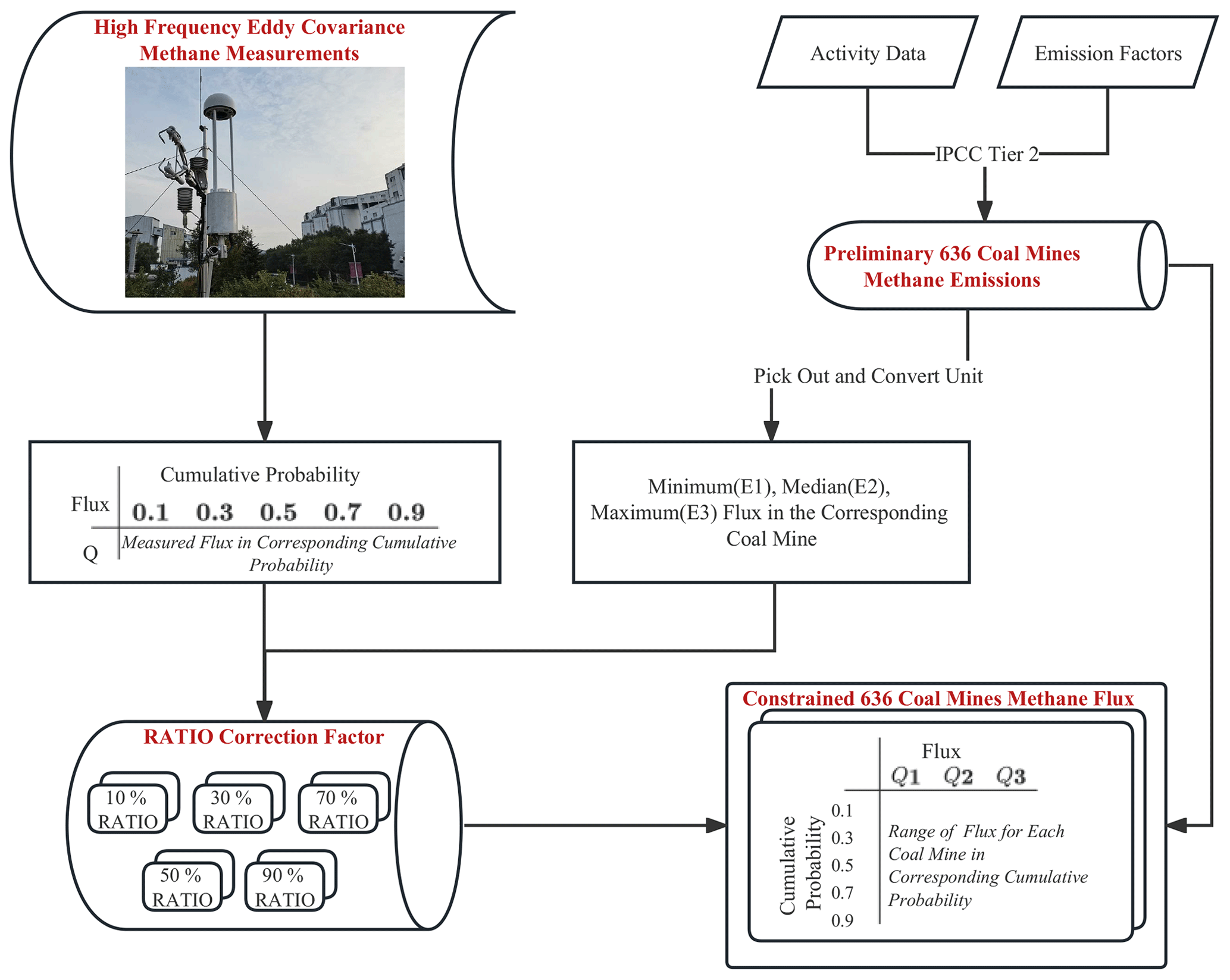
An overview of the methods used in this work is provided in Fig. 1. Measurements of activity data and rank (a qualitative measure of the air flow coming out from the mine) on a mine-by-mine basis are gathered. Different sets of emissions are computed using an approach based on bottom-up technology and geology on a mine-by-mine basis. Simultaneously, 55 d of continuous measurements, taken over two separate periods in 2021 and 2022, using a high-frequency eddy covariance flux tower, is conducted over different seasons of the year at one of the coal mines in the region, which was specifically selected due to its high-quality data and being of typical rank. High-frequency statistics from the flux observations are used to both scale the uncertainty range and compute the bias of the average annual CMM emissions from the mine. There is an explicit consideration of the uncertainties from both the bottom-up and top-down emissions approaches. These correction factors are then applied to the other 635 mines in Shanxi. Emissions in terms of average conditions, temporal variation, and extreme events are quantified. Comparisons are done with other existing bottom-up approaches in terms of space and time, revealing errors and biases in terms of the locations and magnitudes of known, misidentified, and previously missing sources.

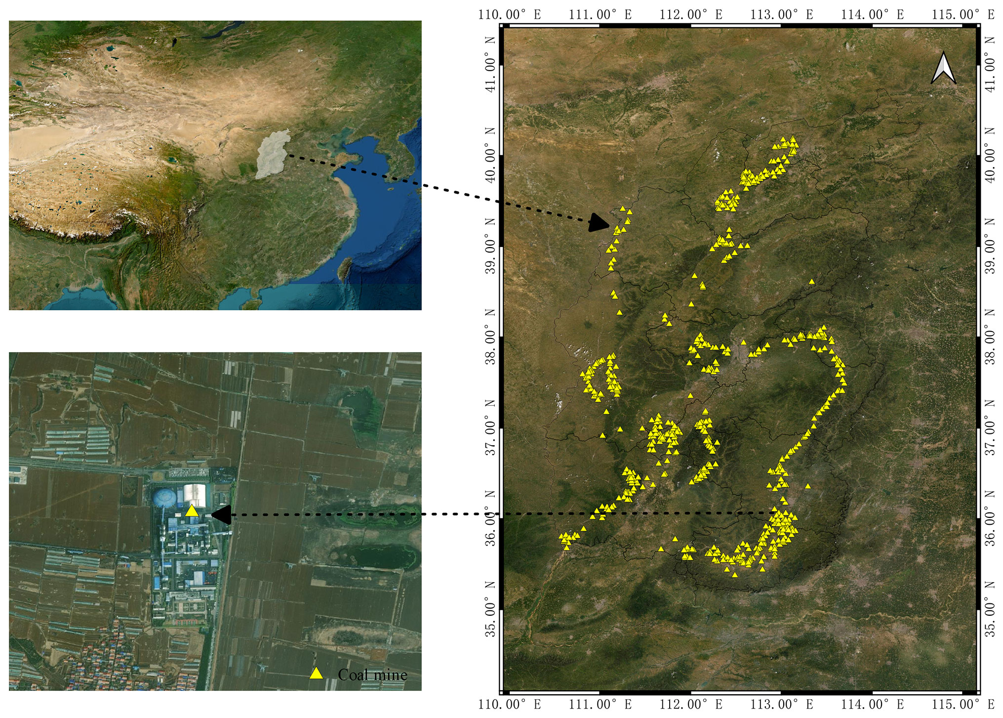
Figure 2 Top left: location of Shanxi within Asia. Right: map of Shanxi with all individual coal mines given as yellow triangles. Bottom left: visible image of an individual coal mine (map from ESRI).

2.1 Geographic boundaries of study region

Shanxi Province in China is one of the major coal-producing regions in the world, currently accounting for 12.0 % of the total global coal output. A map of Shanxi Province and 636 individual coal mines identified in this work is displayed in Fig. 2. The overall geospatial distribution includes both open-pit and underground coal mines, as well as both those mines which are actively in use and others which have already been abandoned.

2.2 Coal mine emissions data

Each mine's location is verified using aerial imagery from ESRI Basemap and Google Earth. The specific geolocation using WGS-84 is presented in Fig. 2.

The bottom-up emissions are computed following the IPCC guidelines for national greenhouse gas inventories' Tier 2 methodology, specifically including a factor of human activity (AD), a coefficient that quantifies the amount of emission per unit of activity (EFs), and a conversion factor (CF) to transform the emissions into units of mass of CH₄. Emissions are conceptually computed following Eq. (1), where EFs (m³ t⁻¹) is the volume of CH₄ emitted per tonne of coal mined and is a function of the activity data used, AD (t yr⁻¹) is the amount of coal produced by each individual mine, and CF is a conversion factor considering the local atmospheric pressure and ideal gas equation (Boettcher et al., 2019).

$$\begin{array}{}\text{(1)}& \mathrm{Emissions}=\text{AD}\cdot \text{EFs}\cdot \text{CF}\end{array}$$

Following the procedures in China, information on the AD is provided on a company-by-company basis, while EFs are computed based on the mine rank. The rank of a mine is determined from the underground observations of the gas and the airspeed of ventilation, the type of gas, and measurements of risk. All coal mines currently in active use in Shanxi Province post detailed information on both their AD and rank, which is available for download at http://nyj.shanxi.gov.cn/mkscnldxgscysxxgg/ggl (last access: 2 December 2021) (there is no English version available), following the approach of the National Mine Safety Administration (2018). In this work, the values of AD are directly used, while four different ranks are used, consisting of “low gas mine”, “high gas mine”, “gas outburst mine”, and “Default”. Each of these ranks corresponds to a specific range of values of emissions factors, as explained in more detail below. Although individual coal mines are required to report the coal mine rank results, only 406 mines analyzed in this work have reported this data, with the authors setting the remaining 230 coal mines to have a “default” rank.

The emission factors depend strongly on the type of coal extracted (for example, but not limited to, brown coal, hard coal, and sea coal), the way in which it is extracted (underground mining versus surface mining), the geological underground structure (which varies based on region-specific observations) and basin uplift history, and the technologies used to extract the coal, among other factors (Zhou et al., 2021). To better constrain the range of emission factors, a literature review was conducted to obtain a range of observed values of EFs as a function of mine rank and type. For surface mines, the EFs were used from Zheng et al. (2005). For underground mines, a set of two to five different values were used, with two papers providing EFs over each of the four ranks (Wang et al., 2013; Gao et al., 2021) and three additional papers providing EFs only over the first three ranks used in this work (Huang et al., 2019; Sheng et al., 2019; Wang et al., 2019), as displayed in Table S1 in the Supplement. This work aims to be technology neutral, and therefore all five values of EFs are considered equally likely for each mine over each of the first three categories of rank. At the mines of default rank, since there are only two different EF values given, a third value is calculated based on the weighted EF values of the low-rank and high-rank mines, with details presented in Table S1. Subsequently all three of these EFs are considered equally likely for each mine in the default rank. The approach used in this work is consistent with previous studies that have been used to derive bottom-up CMM emissions, although there is no previous work that includes as large a number of ranks and different values of EF as employed herein (Huang et al., 2019; Sheng et al., 2019; Wang et al., 2019; Liu et al., 2021). For the purposes of sensitivity analysis this work also calculates the total methane emissions assuming that each mine of default rank also may have EF values the same as high-rank mines, in turn providing an upper bound on the emissions estimation, as compared to the more conservative approach applied herein (Kirchgessner et al., 2000; Wang et al., 2013; Li et al., 2014).

2.3 Methane flux tower data

Measurements of high-frequency CH₄ flux were made at the XiaHuo Village (xhv) coal mine in Zhangzi District, Changzhi, Shanxi Province, China, using an eddy covariance approach (Goulden et al., 1996) with a CSAT-3 anemometer and LI-7700 and generic open-path gas analyzers. The LI-7700 was selected due to its success in constraining CH₄ emissions over terrestrial landscapes (Mcdermitt et al., 2010; Alberto et al., 2014; Peltola et al., 2014; Song et al., 2015; Ge et al., 2018). The observations from LI-7700 are based on a single-mode tunable near-infrared laser capable of operating at ambient temperature. The CH₄ is computed using wavelength modulation spectroscopy (Silver, 1992) across the 1650 nm band and demodulates the resulting signal at twice the frequency. The demodulated signal is compared with a reference signal shape to determine CH₄ concentration (Xu et al., 2010).

The location of the flux tower was placed near the air shaft outflow of a mine that was selected because it is a known source with emissions that are somewhat representative of other “high” ranked mines in Shanxi and therefore would be expected to have both a strong signal and also be a fairly near the middle of the distribution of total coal mines within Shanxi. The Webb, Pearman, and Leuning (WPL)-corrected fluxes are used to compute the emissions flux at 10 Hz frequency, following Webb et al. (1980) and Mcdermitt et al. (2010). These fluxes are subsequently downscaled to half-hourly frequency by averaging over each continuous 30 min block from 24 October to 21 December 2021 and again from 15 August to 13 September 2022. However, some of the observations were uncertain, had irregularities, or otherwise were not trustworthy. When data were not of sufficiently high quality to support the flux calculation via the WPL correction, the data from that entire day were discarded. In total, there are 1544 half-hourly measurements available in 2021 and 667 half-hourly measurements available in 2022, with 55 entire days of data remaining for subsequent analysis.

The absolute value (direction independent) flux, positive only flux, and negative only flux all appear to have similar probability density functions (PDFs), with the only difference being a very minor offset in the positive flux direction. This is consistent with both positive and negative fluxes being actual fluxes associated with the near-surface turbulent flow (Bonan, 2015). Given that there are no other strong sources or sinks of CH₄ within 1500 m except for the coal mine itself, and the coal mine is located at the surface and without buoyancy, both positive fluxes and the absolute value of negative fluxes are retained for this analysis. Therefore, the probability distribution computed using all fluxes on a 30 min average basis is considered from this point forward.

2.4 Ratio correction

There have been multiple studies which have estimated emissions using both top-down and bottom-up approaches and cross-validated the results (Zhang et al., 2018; Long et al., 2021; Ma et al., 2021), but there are few that combine these two methods in tandem (Ho et al., 2019). There are also some hybrid modeling approaches that combine characteristics identified with top-down and bottom-up models but which do not actually use either (Jaccard et al., 2004; Ouyang et al., 2023). This work attempts a new way to perform such a hybrid approach: computing bottom-up emissions following those standard approaches, generating a correction factor between the bottom up emissions and a high-frequency top-down flux observation at a well known and characterized site, and then using this correction factor to apply to all of the other bottom-up emissions datasets to account for both changes in the mean and statistics and high-frequency variation.

A correction factor is computed based on the ratio of each individual half-hourly average computed flux (Q_j) and the average emissions of that mine E_mj. A random sampling of the correction factor is used to generate a PDF of the correction on a half-hourly basis, applied to each local mine's E_mj. Statistics of this factor allow the uncertainty range to be analyzed with respect to temporal variability as well as an objective way to offset and correct any possible bias in both the mean state and its shape as it is distributed over time.

This ratio, $Q_j/E_{\text{m}j}$, was then used to scale the emissions of each individual mine. In particular, the annual average emissions of all other coal mines E_mi were then multiplied by $Q_j/E_{\text{m}j}\cdot E_{\text{m}i}$ point by point, to yield the emissions distribution of each mine i in a probabilistic manner. Since each mine has three to five different possible bottom up emissions inventory values, each of the minimum, maximum, and median cases is scaled. These different initial emissions values, correspondingly E_1j, E_2j, and E_3j, are then applied individually for applications in the rest of this work. The new probability distributions of emissions were gathered mine by mine and condition by condition and outputted with the corresponding flux values (Q_i), specifically calculated for the probability distribution at steps of 10 % from 0.1–0.9 in Table S2.

2.5 Statistical methods

To obtain the probabilistic distribution of emissions for each coal mine, a 10 000 member bootstrap was applied (Felsenstein, 1985). This entails first sampling randomly along the domain from [0,1], corresponding to the cumulative probability. This value was then applied to the PDF of observed CH₄ emissions and then applied mine by mine to compute and apply the ratio correction factor based on the following piecewise procedure. When the random value falls within the range [0.0,0.2], the 10 % ratio is selected; when the random value falls within the range [0.2,0.4], the 30 % ratio is selected; when the random value falls within the range [0.4,0.6], the 50 % ratio is selected; when the random value falls within the range [0.6,0.8], the 70 % ratio is selected; and otherwise the 90 % ratio is selected.

The resulting distributions were then analyzed over groups of mines based on their bottom-up annual emissions amounts as a function of coal mine rank. Confidence intervals for the fluxes at the different percentiles for each individual coal mine and each grouped set of coal mines by rank and their 95 % confidence interval using the bias-corrected and accelerated percentile (Bca) method were computed and are given at https://doi.org/10.6084/m9.figshare.23265644.

2.6 Limitations

The data used to generate the bottom-up emissions are from 2019, while the eddy covariance measurements are made in 2021 and 2022. The EFs are constant from year to year, although there may be interannual variations occurring on a mine-by-mine basis, especially given the unique economic conditions which occurred on the ground in China in 2021 and 2022. There are also uncertainties associated with the variability of the geological conditions encountered as mining expands into new parts of the coal field, and individual mine companies introduce differing new technologies. Since the difference between the high-frequency measured CH₄ fluxes in 2021 and 2022 is very small, and the mines herein have similar geological conditions, this work assumed the observed changes represent the actual observed temporal variation well.

The length of the total dataset was designed to be sufficiently representative of high-frequency variations, such as the effects of different anthropogenic activities occurring at during different times of day and on different day basis, and changes in activities occurring as policies and changes in demand for coal occur. The methods employed here are not sufficiently long to analyze interannual or intraannual variation.

Despite data limitations, the datasets represent an important step forward regarding the spatial and temporal variability of fluxes among individual coal mines. As described herein, many mines are either missing from inventories entirely or found to be located in the wrong place. Second, the data computed in this week are more frequent than the 3-monthly observations made to follow the current policies, which are therefore likely missing with respect to monthly–annual temporal scales of bottom-up emissions processes. This is likely even larger in terms of undersampling-induced biases when using various remotely sensed platforms. However, the length of the dataset and the difficulty of placing a flux tower safely very close to a CH₄ methane output shaft may also lead to a lack of sufficiently broad representation of true emissions, in particular, not successfully sampling all of the extremely high emissions events. For all of these reasons, the results found herein are already likely to be slightly less broad and therefore on average slightly lower than the emissions actually occurring in the real world.

Further limitations stem from the fact that while this work has obtained measurements and locations from 636 different coal mines companies, only 406 contain gas emission rank data. Of these 406 mines containing coal ranks, 259, 122, and 25 mines are respectively defined as being low rank, high rank, and outburst rank. There are also 13 surface mines. According to the China Energy Statistical Yearbook and the Shanxi Energy Balance Sheet, Shanxi Province produced 920.3 Tg of raw coal in 2019, with a total of 915.8 Tg collected. The missing 4.5 Tg of raw coal production implies that there are sites where the geographic location of mines and/or companies are not yet accessible. A part of this confusion may also stem from the fact that 50 coal mines were shut down in 2019 due to various environmental and safety concerns. On top of this, there is one abandoned coal mine that exists in the data. There is likely to be some CMM associated with these sites but which may be outside of the ranges applied in this work to properly analyze.

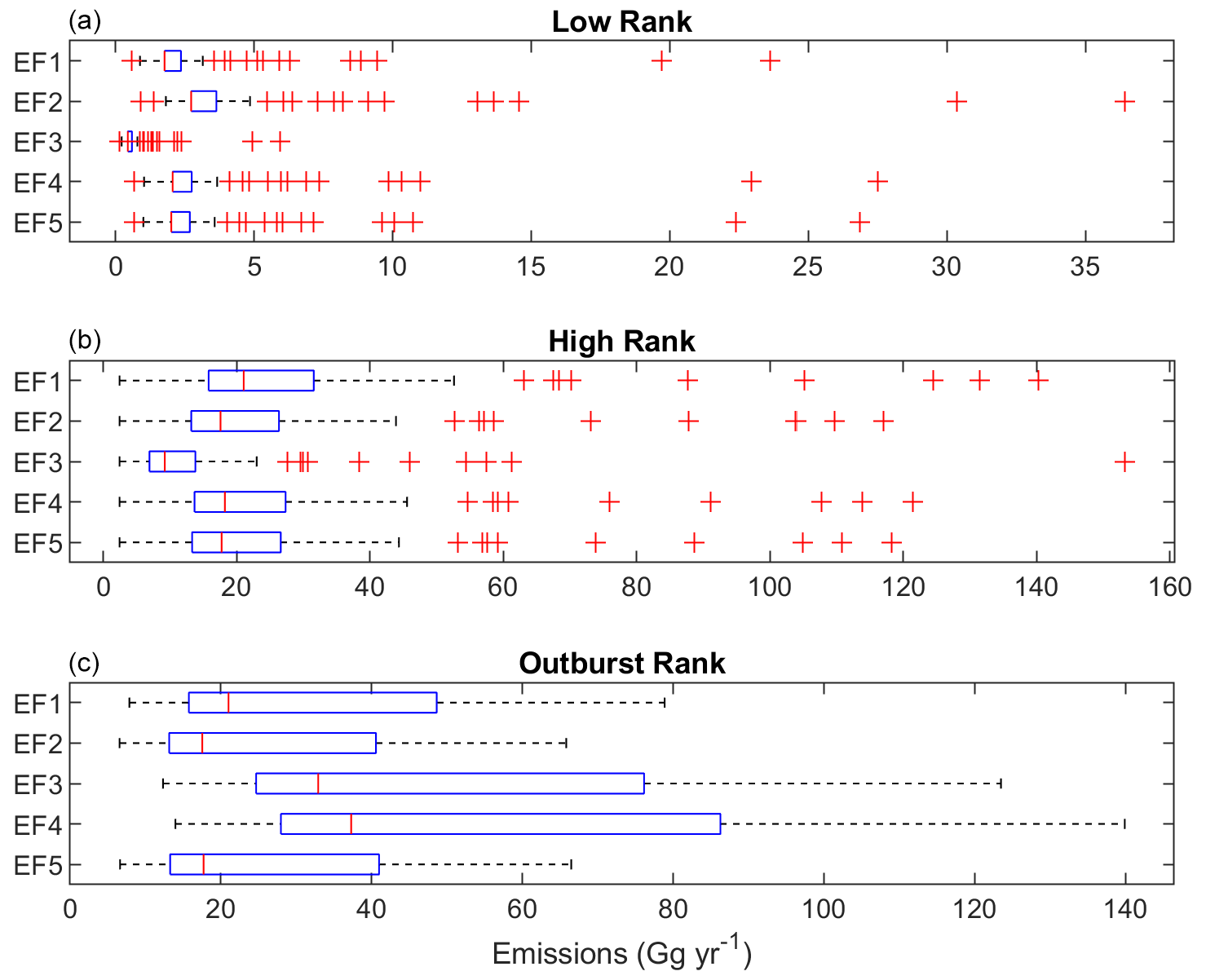
Figure 3 Statistical distribution of bottom-up CH₄ emissions calculated across all mines classified as (a) low rank, (b) high rank, and (c) outburst rank. From top to bottom, each box-and-whisker plot corresponds to EF 1 through EF 5 respectively.

3 Results and discussion

3.1 Initial bottom-up CMM emissions

Using emission factors from Gao et al. (2021), Sheng et al. (2019), Huang et al. (2019), Wang et al. (2013, 2019), and Zheng et al. (2005), in combination with the IPCC Tier 2 approach, the bottom-up emissions from each individual coal mine were calculated. The box plots of the emissions calculated at three different ranks and under five different EFs are shown in Fig. 3. First, it is observed that the central 50 % of emissions values is not always consistent. Under low-rank conditions, the emissions from EF3 are lower than the group consisting of EF1, EF4, and EF5, while EF2 is higher than the other groups. Under high-rank conditions, the grouping of the central 50 % of emissions is slightly tighter, with the EF3 emissions lower than but not statistically outside the group consisting of EF2, EF4, and EF5, although it is statistically lower than EF1. The central 50 % of emissions from EF1 is higher than EF3 but is not outside the range of the others. Under the outburst rank, although EF3 and EF4 are higher than the others, none are statistically located outside of the central 50 % data of the others. The CMM emissions are quite broad across each rank, with a range from 0.15–36.4 Gg yr⁻¹ at low rank, from 2.41–153 Gg yr⁻¹ at high rank, and from 6.58–140 Gg yr⁻¹ at outburst rank. All statistics are provided in Fig. 3.

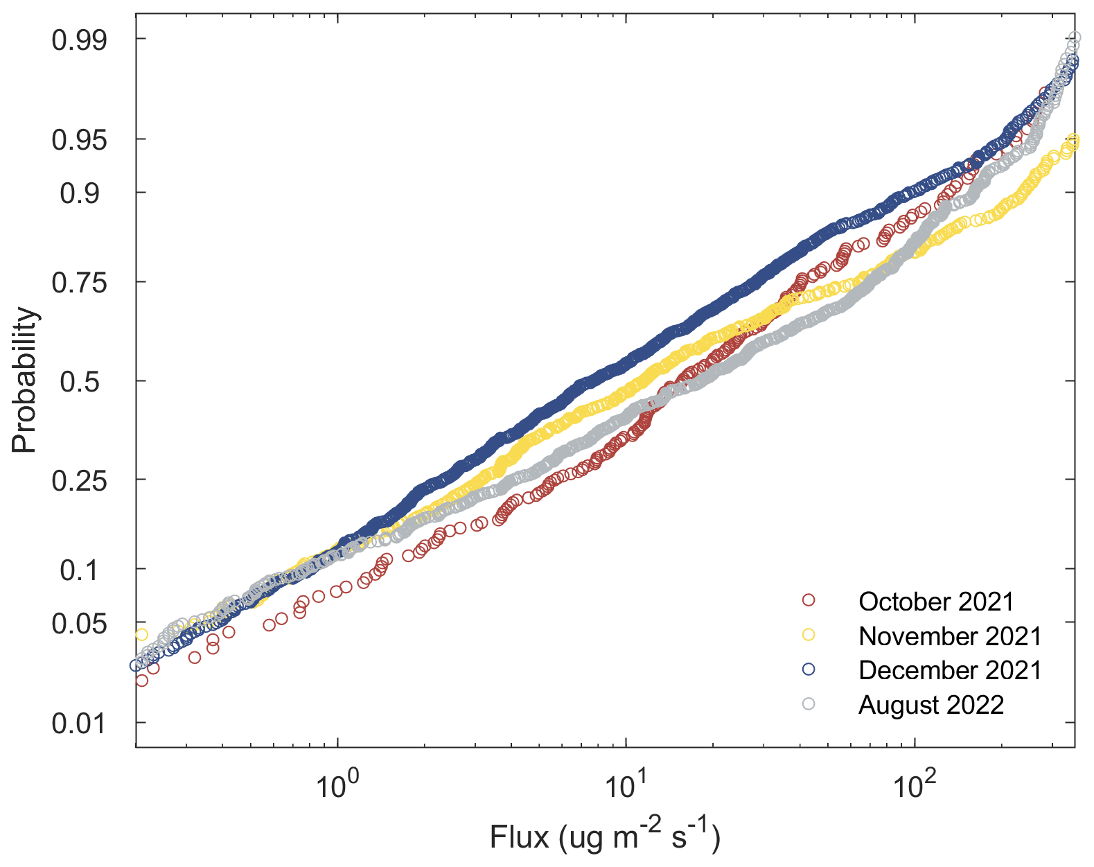
Figure 4 Cumulative probability distribution of 30 min eddy covariance flux measurements (µg m⁻² s⁻¹), where red is October 2021, yellow is November 2021, blue is December 2021, and grey is August 2022. All observations are included in this plot.

On a Shanxi-wide basis, the range of bottom-up emissions, with the 10th to 90th percentile range of 0.35–1.82 to 13.8–29.6 Gg yr⁻¹, was found to be broader than other works which have estimated CMM, which range from a low of 4.41 Tg yr⁻¹ to a high of 7.77 Tg yr⁻¹ (Wang et al., 2013, 2019; Huang et al., 2019; Sheng et al., 2019; Gao et al., 2021). The results also are found to be broader than the most widely used bottom-up emission inventories produced using global-scale data for CH₄: EDGAR (Oreggioni et al., 2021; Janssens-Maenhout et al., 2019) v6 (Crippa, 2021) and GFEI (Scarpelli et al., 2022, 2020) v2 (Scarpelli and Jacob, 2021), which have a 10th and 90th percentile range of 0.77 to 30.1 Gg yr⁻¹ and 0.02 to 12.9 Gg yr⁻¹ in Shanxi respectively.

The reasons that this work's results are broader than previous works are in part because this work uses multiple independent input databases, while Sheng et al. (2019) and Gao et al. (2021) calculated emissions factors derived from the State Administration of Coal Mine Safety (SACMS), Wang et al. (2019) calculated data from the China High Resolution Emission Gridded Database (CHRED), and Huang et al. (2019) derived their emission factors from Yuan et al. (2006), which in turn were calculated form the same underlying national level statistics, with data of large key enterprises in China used as supporting data. The reason that EF3 is statistically lower than every other EFs at low rank and is statistically lower than EF1 at high rank may be in part for two reasons: first, this work does not consider a separate factor for abandoned mines and open-pit mines, while second, this work uses a unified gas level statistic for low- and high-rank mines (Wang et al., 2013). As discussed later in this work, there is further divergence induced by both geospatial and temporal differences between EDGAR and GFEI on the one hand and the high-resolution maps with scaled high- frequency methane measurements on the other hand, as demonstrated by the maximum and minimum values of EDGAR being (0. and 712.) and GFEI being (0. and 200.) Gg yr⁻¹ respectively, far outside of the range of the results herein, even at the highest emitting mine.

3.2 Eddy covariance emissions

The cumulative distribution functions (CDFs) of 30 min eddy covariance observations on a month-by-month basis are given in Fig. 4. First, it is observed that the flux in December 2021 is always lower than in the other months, by an average value of 20.4 µg m⁻² s⁻¹. The other 3 months have similar mean and median values, with there being only small differences in different probability regions. Specifically in the percentile range around 44.8 %, the flux in August 2022 is at most 2.62 µg m⁻² s⁻¹ lower than in October 2021, and the flux in the percentile range near 68.9 % in November 2021 is at most 5.60 µg m⁻² s⁻¹ lower than in October 2021. Even considering the absolute shift between December 2021 and the other months, the magnitude is relatively small compared with both the median and variance. Therefore, the sampling time is assumed to be sufficient to represent the actual variability in the observed CMM flux over the duration when the observations were made.

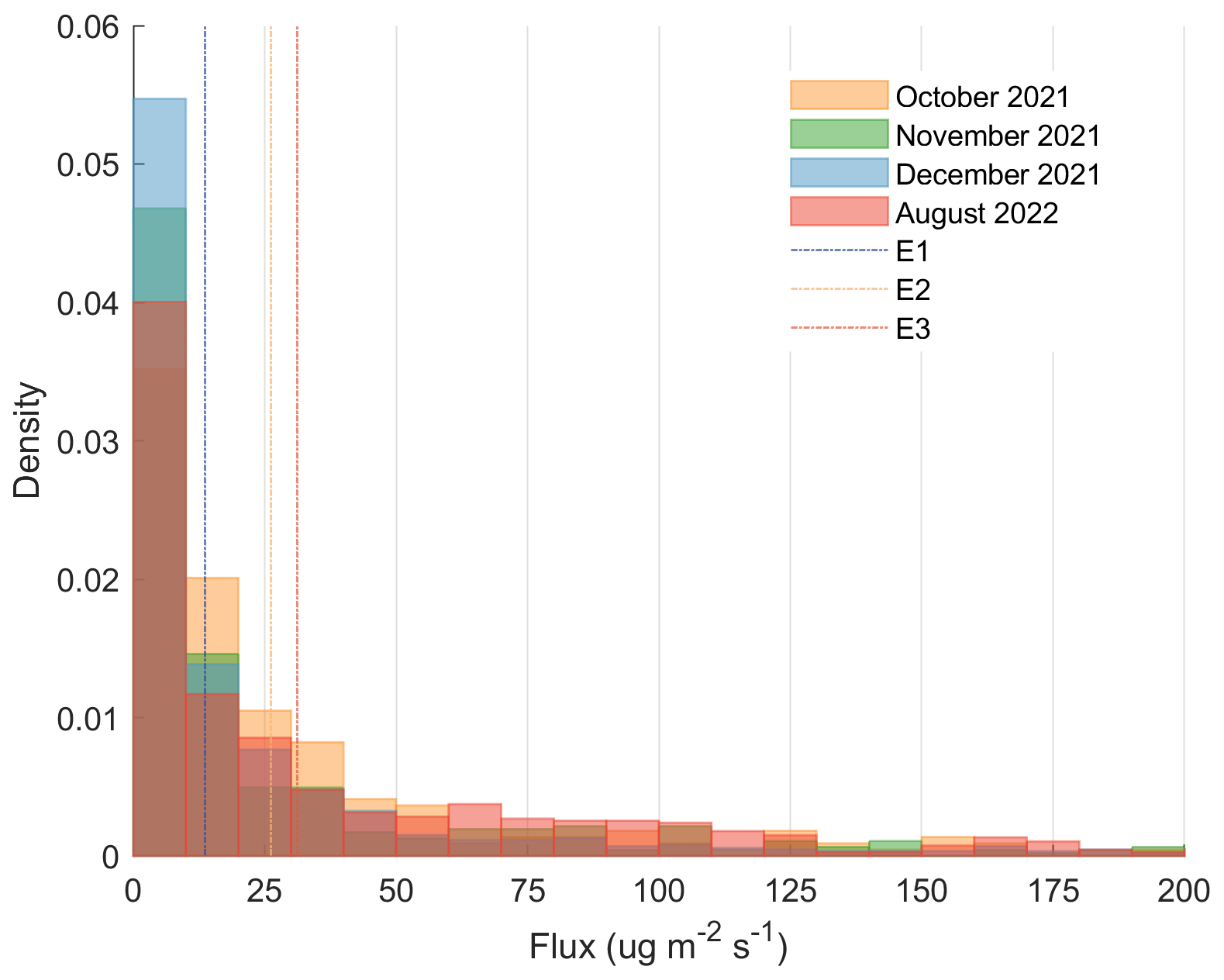
Figure 5 Probability density functions of eddy covariance fluxes (in µg m⁻² s⁻¹) are given as different colored bars over different times: orange is October 2021, green is November 2021, blue is December 2021, and red is August 2022. Bottom-up emissions fluxes in µg m⁻² s⁻¹ for E₁, minimum flux; E₂, median flux; and E₃, maximum flux, are given as light-blue, yellow, and red dashed–dotted vertical lines respectively. Fluxes higher than 200 µg m⁻² s⁻¹ are not shown.

The observed fluxes are presented as a PDF along with the three bottom-up emissions estimations for the same (xhv), presented in Fig. 5. The three vertical lines respectively correspond to the minimum (E₁), median (E₂), and maximum (E₃) bottom-up emission values calculated in Sect. 3.1, which are respectively 13.6, 26.3, and 31.1 µg m⁻² s⁻¹. While the distribution is clearly skewed, it is not biased, with the boxes covering E₁, E₂, and E₃ representing the central 15.5 % of data, 53.5 % of the data falling into the single box below E₁, and 31.0 % of the data within the remaining boxes above the ceiling of the bottom-up measurements. Similar to Frankenberg et al. (2016), this work's observations have a long tail and are approximately lognormally distributed.

The bottom-up approach slightly overestimates the median of the emissions distribution (11.7 µg m⁻² s⁻¹), although it also simultaneously underestimates the mean of the emissions on a mass basis (50.4 µg m⁻² s⁻¹) due to the top 14.4 % of emissions being an order of magnitude higher than the median range. This means that an insufficiently large sample, such as that which may be made by infrequent overpasses by high-resolution satellites or highly intensive but short-duration field campaigns, risks leading to a biased overall representation of the emissions. Since the data are sufficiently representative of the overall distribution of bottom-up sources on a daily scale, the randomly sampled variability of the measurements as a whole is assumed to be a measure of the true variability in time, and this relationship is then applied on a day-to-day basis to scale the annually distributed emissions for further analysis.

The rest of this work outlines the use and impact that scaling the annualized emissions and its uncertainty range on a mine-by-mine basis have using the high-frequency variance in time applied in a probabilistic manner. These scaled emissions impact both the magnitude and variability of E₁, E₂, and E₃ to make them consistent with the statistics and variability of the observations, leading to a new dataset of emissions constructed of all coal mines in Shanxi that shares the same probabilistic variability observed at xhv. This is reasonable given that the high-frequency variability is likely linked to the common geology, economic, and technological conditions found throughout the province and not due to other external sources, different policies, or differences in how the coal is mined and/or processed.

3.3 Constrained CMM emissions

The ratio correction factors were applied to every coal mine after conversion of units from Gg yr⁻¹ to µg m⁻² s⁻¹, by assuming the area to be that of the property owned by each coal mining company. In the case where individual mines do not contain sufficient information needed to successfully convert units, this work uses average unit conversion values, computed grouping the remaining mines by their rank, with 149 of the total of 636 coal mines falling into this category. For those mines with sufficient information, bootstrap simulation was used to obtain the confidence interval (CI) around the mean. This work then randomly selected data from the central 95 % of the CI corresponding to the rank of the coal mine.

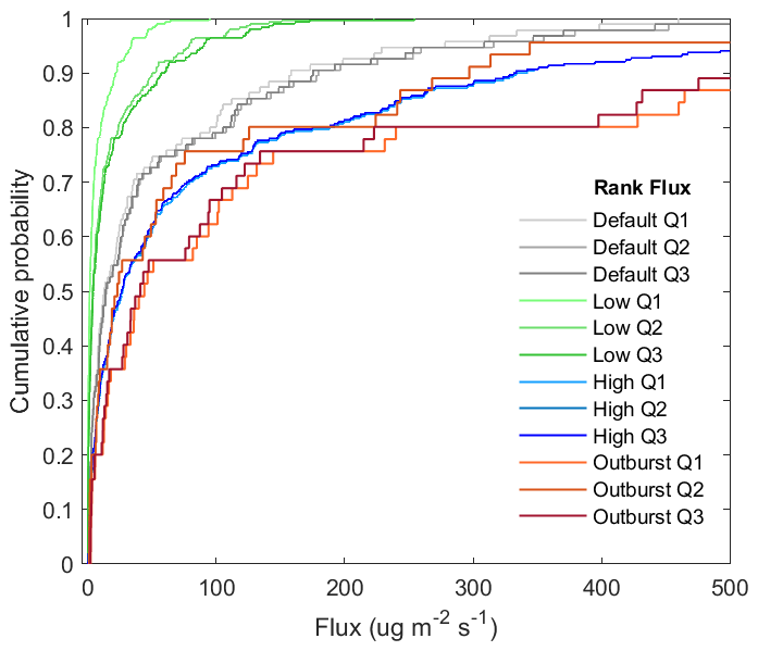
Figure 6 CDFs of emissions as a function of different ranks (µg m⁻² s⁻¹). Rank and Q_j (j=1, 2, 3), which are defined and described in Sect. 2.2 and 2.4 respectively.

Figure 6 shows the CDF of emissions fluxes as a function of different ranks and technology levels. Each rank has three curves (Q_j, j=1, 2, 3), corresponding to the base cases E₁, E₂, and E₃, with details and statistics of constrained CMM fluxes presented in Table S2. As can be seen across each rank (except for Outburst) that E₁ always has the lowest emissions, E₂ always has intermediate emissions, and E₃ always has the highest relative emissions. With respect to the rank, while low is always lower than default, and default is lower than high or outburst, high and outburst are not always lower or higher than each other. While these findings are generally consistent with the idea that the rank of a coal mine is related to its emissions, there are exceptions to this general rule. Since the current treatment of default rank is a linear weighting of low-rank and high-rank functions, this itself can be further modified in terms of how many different coal mines there are in each respective weight, allowing the end user of the emissions to rapidly override the assumptions made herein and use the default rank to define any new rank that the user may want.

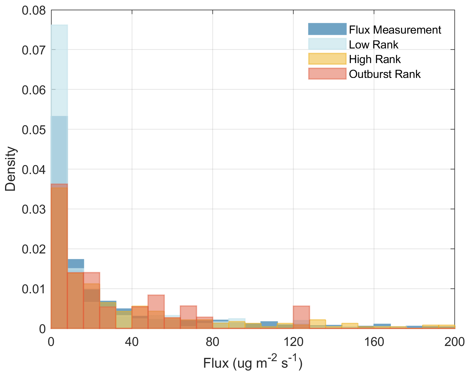
Figure 7 PDF of all calculated emissions fluxes across all mines, separated rank by rank in units of µg m⁻² s⁻¹, where light blue is low rank, yellow is high rank, and red is outburst rank. PDFs of flux observations less than 200 µg m⁻² s⁻¹ are given in dark blue.

PDFs of emissions across all mines on a mine-by-mine basis are analyzed for different ranks in Fig. 7. First, it is clear that the low-rank fluxes are lower than the observations. Second, fluxes at both high and outburst ranks generally are found to be larger than the flux observations. However when only considering the set of super-high emissions (herein considered to be larger than 100 µg m⁻² s⁻¹), these conditions consist of 26.5 % of mines with high rank, 22.1 % mines with outburst rank, and 14.4 % of the observed fluxes.

3.4 Comparison with existing inventories

The results from this study are compared with multiple existing community emissions databases of CMM that are built using the bottom-up approach including EDGAR, GFEI, US-EPA Community Emissions Data System (CEDS) (Mcduffie et al., 2020; Hoesly et al., 2018), and Peking University Emissions database PKU-CH₄ (Liu et al., 2021; Peng et al., 2016). These different datasets estimate their emissions using a consistent approach based on country-specific activity data, emissions factors, and technological abatement when available and claim to cover all major source sectors, including fossil fuels, and therefore should be capable of representing CMM emissions. The notable differences include EDGAR mostly applying a Tier 1 approach, GFEI applying a hybrid Tier 1 and Tier 2 approach depending on data availability, and CEDS scaling pre-existing emissions to match country-specific inventories already reported to the UNFCCC. For these reasons, the different databases can differ from each other in terms of sector-by-sector coverage, geospatial distribution, temporal averaging, uncertainty range, and how the emissions are mapped, among other differences.

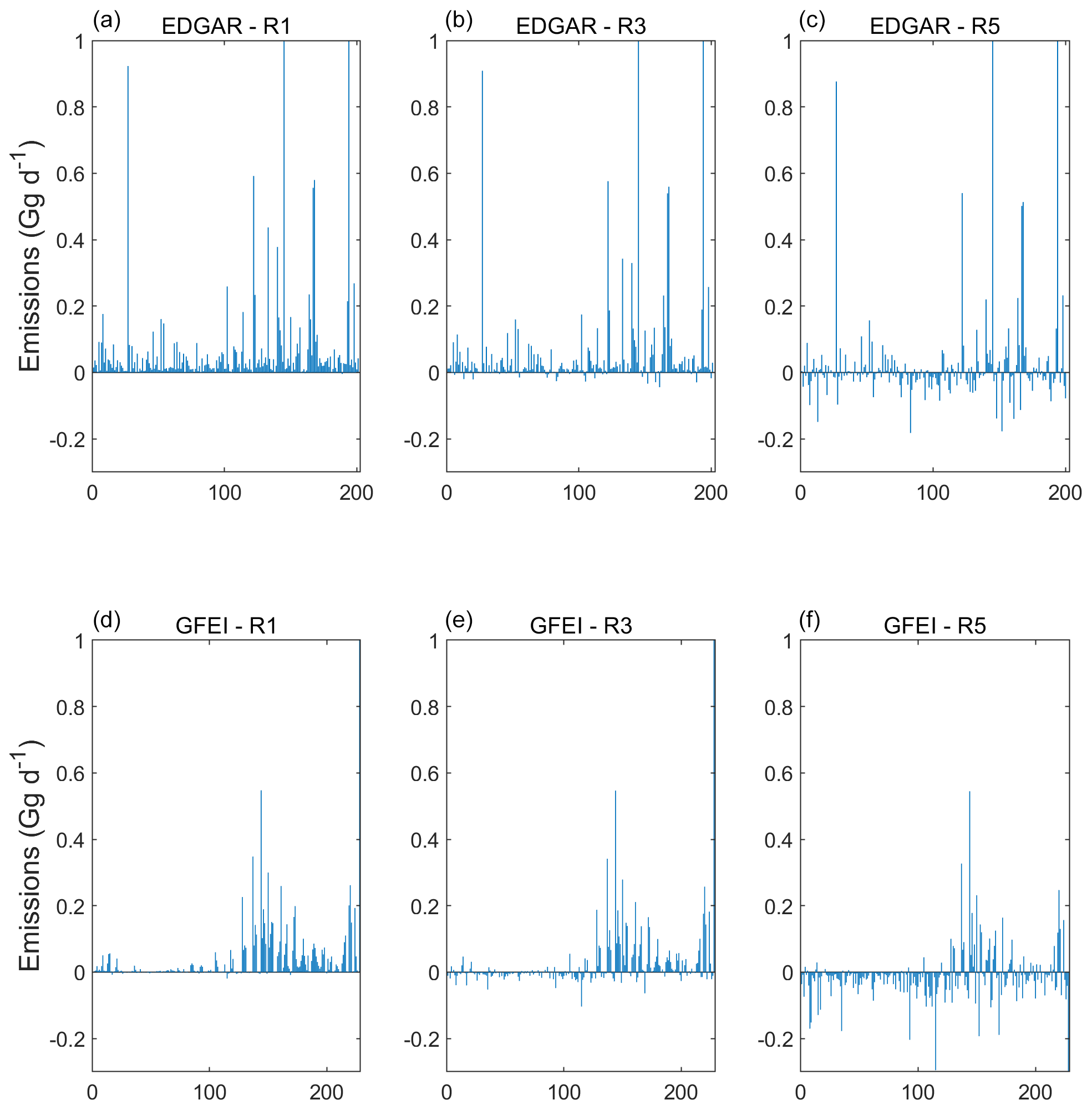
Figure 8 Grid-by-grid difference between EDGAR (a–c) or GFEI (d–f) and this work's respective corrected emissions (a, d) R1, (b, e) R3, and (c, f) R5, with y axis in units of Gg d⁻¹ and x axis corresponding to each individual grid.

EDGAR is a bottom-up global database of anthropogenic emissions of greenhouse gases and air pollutants that provides estimates based on data reported by European member states or by parties under the UNFCCC, using the IPCC methodology. EDGAR provides emissions of CH₄ at 0.1°×0.1° spatial resolution and both monthly and annual time resolution over the domain studied (Crippa, 2021). GFEI allocates methane emissions from oil, gas, and coal at 0.1°×0.1° spatial resolution using the national emissions reported by individual countries to the UNFCCC and mapping them to infrastructure locations (specifically using IPCC sectors 1B1 and 1B2) (Scarpelli and Jacob, 2021). This work makes specific comparisons between the computed CMM emissions and results using EDGAR version 6.0 and GFEI version 2.0. First, all individual mines were summed together on the same spatial grid used by EDGAR and GFEI at 0.1°×0.1° on a grid-by-grid basis, with the results shown in Table 1. Cases in which this work's results are both larger than and smaller than EDGAR and GFEI results are individually analyzed, and differences in the probability distribution of emissions corrected by 10 %, 30 %, 50 %, 70 %, and 90 % are individually included as R1, R3, R5, R7, and R9. Note that all values are computed in terms of Gg d⁻¹, so as to represent the actual variability in the observations made herein and to understand more deeply how annual and other long-term averages may not be precise without appropriate sampling techniques. While the 90 % values look to be quite large, there are many accounts in the real world which match these values, including flux tower observations (Xu et al., 2014), a 20 d study of a well blowout from Ohio which was reported to account for a quarter of the state's annual methane emissions (Pandey et al., 2019), and a large single day's emissions from an undersea gas pipeline explosion (Yu et al., 2022). Therefore, the 90 % values provide an essential quantification of low-probability high-emitting events that actually occur in the real world.

Table 1 Statistical comparison of emissions in Gg d⁻¹, production in Tg, grid numbers, mine numbers, and rank.

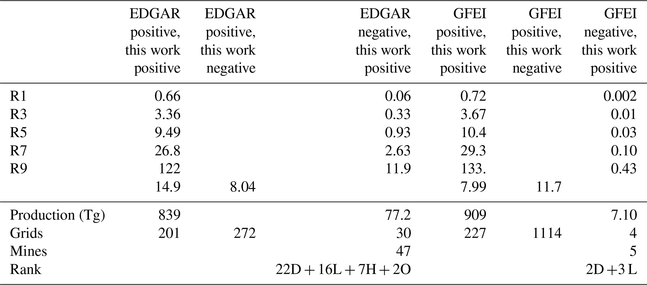
Throughout Shanxi, 201 grids have non-zero CMM emissions both from this work and EDGAR, with respective R5 and EDGAR emissions of 9.49 and 14.9 Gg d⁻¹, while 227 grids have non-zero CMM both from this work and GFEI, with respective R5 and GFEI emissions of 10.4 and 7.99 Gg d⁻¹. There are 272 grids where EDGAR has non-zero CMM, while this work shows no coal mines, with total emissions of 8.04 Gg d⁻¹. There are 30 grids where this work has non-zero CMM and EDGAR has no emissions, with a resulting R5 value of 0.93 Gg d⁻¹. These grids contain 47 mines, of which 22 are default rank, 16 are low rank, 7 are high rank, and 2 are outburst rank, accounting for a total raw coal production of 77.2 Tg. There are 1114 grids where GFEI has non-zero CMM, while this work shows no coal mines, with a total emissions of 11.7 Gg d⁻¹, between our R5 and R7 values. There are four grids where this work has non-zero CMM and GFEI has no emissions, with a resulting R5 value of 0.03 Gg d⁻¹. These four grids contain five mines, of which two are default rank and three are low rank, accounting for a total raw coal production of 7.10 Tg.

Mine-by-mine differences between EDGAR, GFEI, and this work's CMM are respectively shown in Fig. 8, where the x axis represents each individual grid that contains non-zero emissions of both datasets, and the y axis represents the difference of EDGAR/GFEI – our CMM emissions in units of Gg d⁻¹. EDGAR has 7 grids with values much smaller than R1 (in total summing to 0.014 Gg d⁻¹); 66 grids with values between the R3 and R5 values; and a very small number of grids, 12, larger than the R9 values. GFEI has 58 grids with values much smaller than R1 (in total summing to 0.13 Gg d⁻¹); 55 grids with values between the R3 and R5 values; and a very small number of grids, 10, larger than the R9 values. This work's Shanxi-wide results have a bottom-up CMM range of E₁ to E₃ ranging from 4.41–7.77 Tg yr⁻¹ and a post-correction CMM emissions range at R3, R5, and R7 respectively of [1.35,3.81,10.75] Tg yr⁻¹. While both EDGAR and GFEI summed Shanxi-wide emissions are larger than R5 and smaller than R7 values, this is not the case when those locations at which there are no mines are removed. EDGAR has a Shanxi-wide CMM of 8.38 Tg yr⁻¹, of which the CMM at locations without mines is 2.94 Tg yr⁻¹. GFEI has a Shanxi-wide CMM of 7.19 Tg yr⁻¹, of which the CMM at locations without mines is even larger, 4.27 Tg yr⁻¹.

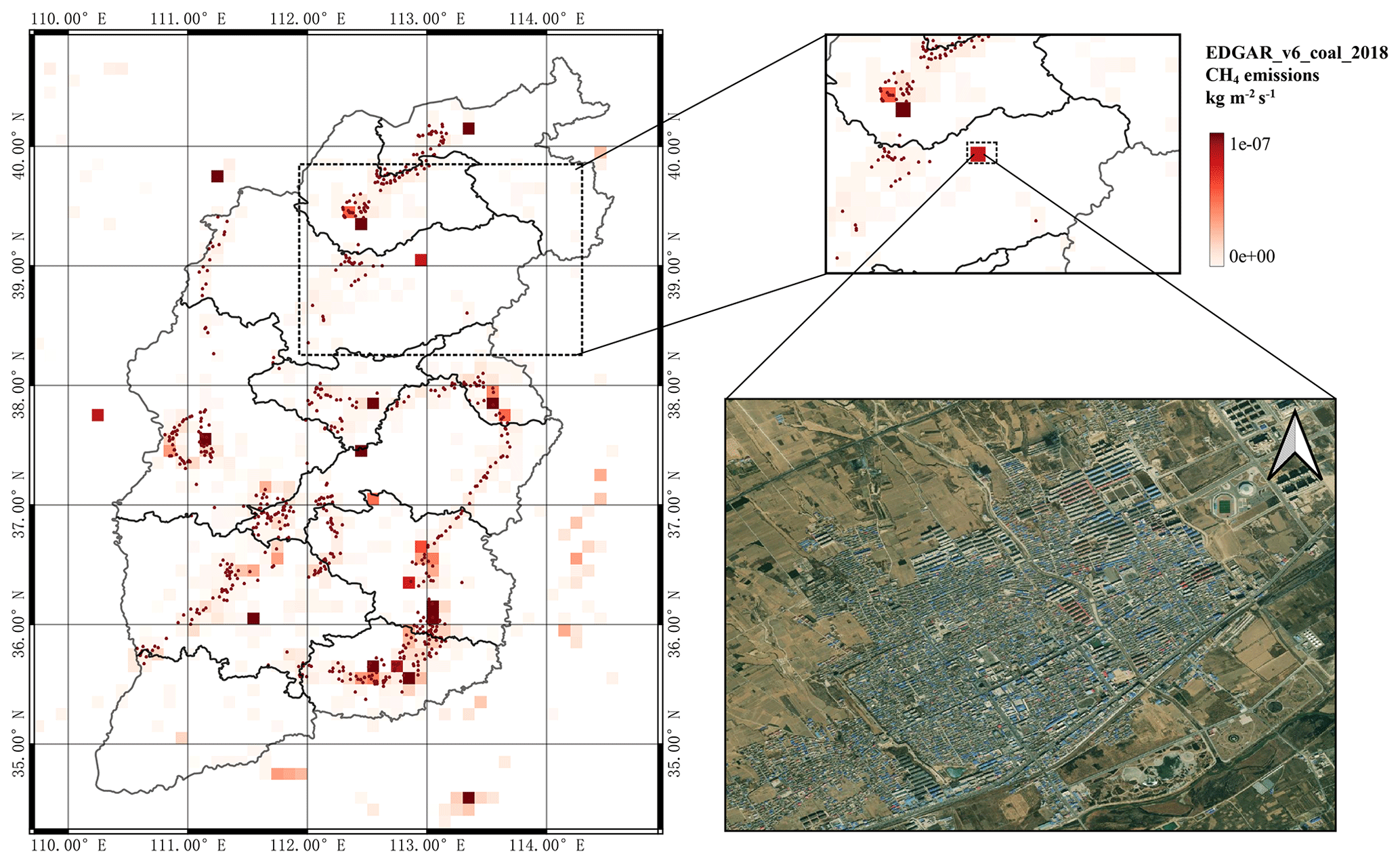
Figure 9 The mapped annual average emissions from EDGAR are overlapped with the locations of the mines used in this work. Note that the region located inside of the dashed black box is shown in more detail on the top right as an EDGAR CH₄ emissions hotspot. However, there are no actual coal mines anywhere in the box. This is supported by the RGB image (from ESRI) of the actual location, which shows a residential area.

To visualize the spatial differences, maps of the grid-by-grid annual average emissions from EDGAR and GFEI are overlapped with the locations of the mines used in this work in Figs. 9 and 10 respectively. A deeper investigation is done into two sets of regions: those in which this dataset has emissions and there are no emissions in one or both of EDGAR or GFEI and those regions in which there are no coal mines, but one or both of EDGAR and GFEI have emissions. Both sets of improperly mapped emissions are indicative of systematic bias or error and can not be corrected merely through scaling (Cohen et al., 2011).

Throughout Shanxi, GFEI shows no emissions at 5 mines and extremely low emissions at 5 more mines, while EDGAR shows no emissions at 47 mines and extremely low emissions at 38 additional mines. One specific and fascinating detail to investigate is that the grid in which this work's flux tower measurements of CH₄ were made (where xhv is located) happens to be one of these special grids. EDGAR reports zero emissions, and GFEI reports very low emissions, 5.28 µg m⁻² s⁻¹, while our E₁ value is 13.6 µg m⁻² s⁻¹, and our corrected 30 % ratio is 4.13 µg m⁻² s⁻¹.

For this reason, a comparison on a grid-by-grid and mine-by-mine basis over the entire city of Changzhi is conducted. The Changzhi-wide statistics of (minimum, median, maximum, and mean) emissions of EDGAR on a grid-by-grid basis where coal mines exist are 0.12, 5.29, 67.7, and 13.2 µg m⁻² s⁻¹, respectively, while their same statistics within Changzhi on grids which do not have coal emissions are 0.18, 0.55, 36.9, and 4.38 µg m⁻² s⁻¹. This work's CMM inventory at xhv has values of E₁ to E₃ ranging from 13.6–31.1 µg m⁻² s⁻¹, with the corresponding final 10 %, 30 %, 50 %, 70 %, and 90 % emissions values after ratio correction being [0.81,4.13,11.7,33.0,150] µg m⁻² s⁻¹, respectively. This indicates that the EDGAR emissions in general have both a lower mean and a narrower distribution as compared with the results within Changzhi, as well as a significant fraction of urban CH₄ emissions misidentified as being due to fossil fuels.

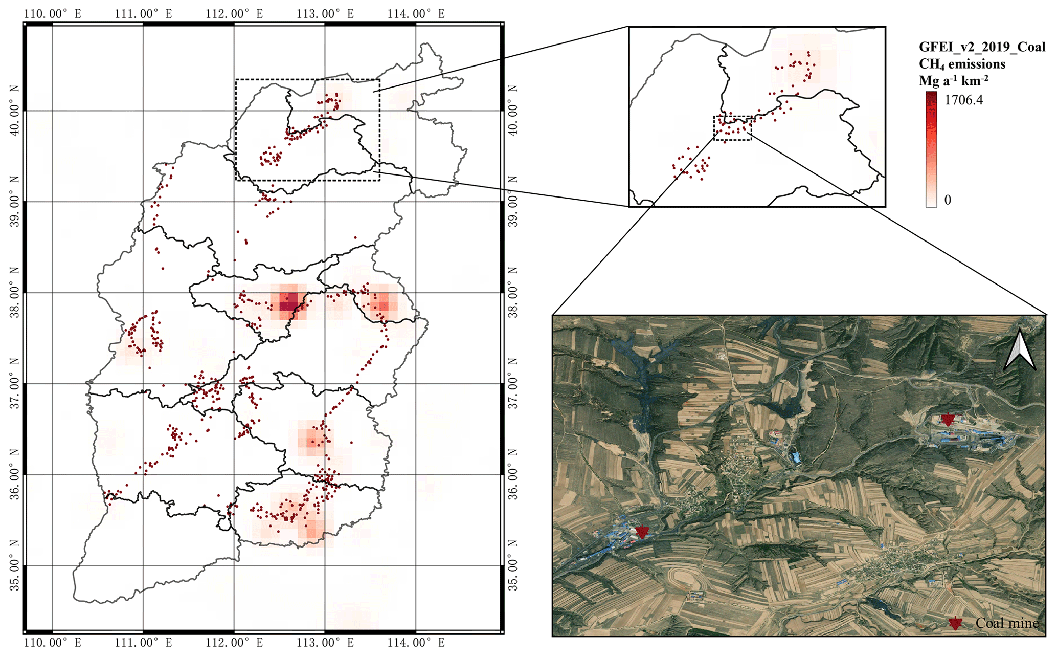
Figure 10 The mapped annual average emissions from GFEI are overlapped with the locations of the mines used in this work. Note that the region located inside of the dashed black box is shown in more detail on the top right as a region with almost zero emissions by GFEI CH₄ emissions. However, the actual location contains multiple coal mines. For ease of viewing, only 2 of the 25 coal mines are shown on the map (from ESRI).

A map of the grid-by-grid average GFEI CMM emissions is overlapped with the locations of the mines used in this work in Fig. 10. As observed, there are some regions which exist in GFEI which also exist in our dataset, there are other regions in GFEI which are not identified in our dataset, and there are regions identified in our dataset which do not exist in GFEI. As demonstrated in Fig. 8, some of the regions containing mines in this work have effectively almost no emissions as reported by GFEI, indicating that there is likely a spatial mismatch. The total emissions in regions which have mines but are not reported by GFEI range from 0.74–10.1 Gg yr⁻¹ at E₁ and from 1.77 to 14.72 Gg yr⁻¹ at E₃.

In the subregion shown in Fig. 10, GFEI reports emissions at six grids, with a range from a minimum of 0.17 Gg yr⁻¹ to a maximum of 0.59 Gg yr⁻¹. This work's total emissions over the mines reports emissions at five of these grids, while there are none reported at the largest GFEI grid within this region (0.59 Gg yr⁻¹). The emissions calculated by this work's approach at the minimum of these GFEI grids (0.17 Gg yr⁻¹) are computed to have a 30 %, 50 %, and 70 % value of 10.3, 29.2, and 82.3 Gg yr⁻¹, respectively, while the emissions at the maximum of these GFEI grids (0.58 Gg yr⁻¹) are calculated to have a 30 %, 50 %, and 70 % value of 12.4, 35.2, and 99.3 Gg yr⁻¹. These findings show that scaling GFEI will not lead to a good match with the CMM emissions, since the orders of magnitude of the observed mine-by-mine emissions are not the same as the GFEI emissions, and even using different scaling factors for different rank mines would also be insufficient.

There are regions identified in this work at which GFEI and EDGAR both have very high emissions, in which there is actually a large urban center (eastern Taiyuan) or industrial center (southwestern Linfen and northeastern Xinzhou), all without any mines. Another work (Li et al., 2023) identifies industrial boilers as the major source of emissions in one of these regions, some of which are powered by natural gas. Whether such a spatial mismatch or mis-identification has occurred, or a more fundamental error in how the CH₄ emissions are partitioned for industrial sources, is unfortunately not provided by the EDGAR or GFEI teams and can not be investigated further.

Following the results of Brandt et al. (2014), measurements at all scales show that official inventories underestimate actual CH₄ emissions conservatively defined as 1.25–1.75 times EPA GHGI estimates. For this reason, the R7 value obtained in this work, which is about 1.3–2.4 times higher than bottom-up estimates in coal mining sector, seems to be a decent fit. This concept of official inventories underestimating CMM is further highlighted by the issue of emissions from closed coal mines. Even though the number of coal mines being stopped due to various regulations is increasing, it seems that the quantification of abandoned mine methane (AMM) emissions is not considered reasonable. In this work a single abandoned mine is identified, and its R3, R5, and R7 emissions are calculated to be 0.48, 1.35, and 3.81 Gg yr⁻¹, much larger than the China-wide AMM emissions of 4.7 ± 0.94 Tg in 2020 produced by Chen et al. (2022).

While there are many such papers making claims that top-down estimates of CH₄ emissions are slightly lower than bottom-up approaches at global scale (i.e. Saunois et al., 2020), there are no actual data available over Shanxi Province, and therefore, such a comparison is not possible at the present time. However, Maasakkers et al. (2022) used TROPOMI data to invert CH₄ emissions at a city-level spatial scale and found that the emissions are 1.4 to 2.6 times larger than reported in commonly used emission inventories. While this compares reasonably on average with our mine-by-mine values over the range from R5 to R7, as already detailed above, a more precise grid-by-grid approach is required to make a thorough comparison, since otherwise mis-attribution may play a significant role.

4 Conclusions

This work has compiled a mine-by-mine and high-temporal-resolution inventory of Shanxi Province's 2019 CMM emissions. This inventory provides a specific location for each coal mine, including inactive mines. The technology-based approach first employed produces a range of emissions from 4.41–7.77 Tg CH₄ in 2019. To explore the impact of relaxing this assumption, substituting the EF from high gas mines instead of the more conservative weighted mixture approach was used to determine an upper-end constraint on the overall methane emissions. The total net increase in emissions is computed to be 1.71(1.67–1.82) Tg over Shanxi as a whole, leading to a final net total emission of 4.41–9.47 Tg. The follow-up approach of scaling the observations based on the PDF analysis of high-frequency eddy covariance methane measurements was proposed as a correction. This set of ratio correction factors was applied and yielded a set of emissions at the 10 %, 30 %, 50 %, 70 %, and 90 % level of [0.72,3.69,10.4,29.4,133] GgCH₄ d⁻¹. By preparing a PDF, such extreme events as occasionally observed can also be analyzed, consistent with the eddy covariance observations which show a lognormal distribution.

Comparison between our bottom-up inventories with EDGAR and GFEI reveals that a proper spatial and temporal comparison is essential. While on a province-wide basis both EDGAR and GFEI lie between this work's 50 % and 70 % values, with EDGAR closer to our 70 % value than GFEI, this is not a spatially coherent comparison. While looking only at the geospatial grids which actually contain coal mines, both EDGAR and GFEI are found in our 30 % to 50 % range, and therefore both underestimate the median emissions. Furthermore, in both cases, on a mine-by-mine basis, the values are generally found to be slightly too low, while there are also some mines which are an order of magnitude or more too high. On top of this, both datasets have a considerable amount of CMM observed in regions which are urban, or which are commercial, and which do not have any mines. This indicates that in general the values of EDGAR and GFEI CMM Shanxi-wide that are slightly too low are due to a few serious distortions. Specifically, these datasets generally have a low bias and underestimate CMM on the vast majority of grids in which there is overlap. The datasets then offset this bias in two ways: first through a systematic overestimation of CMM on some grids at the high end of the distribution and second through including emissions on a large number of grids which do not actually have any coal mines. For this reason, it is essential to analyze the total emissions not only on an overall basis but also in terms of location, magnitude, and variability, otherwise comparisons with and validation using remotely sensed products and models become a case of comparing things that may have the same name but are actually quite different.

The scaling done in this work is based on 55 d of observations at a single large coal mine. While the results seem relatively consistent month to month, the variability may be found to also exhibit a different characteristic if additional sites are analyzed. Furthermore, analyzing different types of sites based not only on production but also based on different underlying geological conditions or methods by which the coal was extracted may also provide deeper insights. Given that the wind patterns are different in this region during different phases of both El Niño and La Niña, as well as other dynamical regimes (Baldwin et al., 2001), continuing to measure data over a longer period of time may lead to a further refinement of the probability distribution of the observed fluxes. On top of this, mining leakage or procedures may be different in very cold months from very hot months, and therefore a better representation of the emissions under different temperature conditions, especially with respect to how they change the different mining procedures, may also help to improve the accuracy. The goal is to provide enough data and cover enough cases, so as to offer the most improved possible set of observations, so that the more broad and well-supported range of emissions can be constrained, allowing for ultimate development of CMM mitigation.

Comparisons with existing CMM emissions are shown to demonstrate greater spatial and temporal variability, national and international inventories and carbon accounting, and more process and model refinement and development. Although aggregated emissions are generally of the same order of magnitude at the province level, there are quantitative differences observed in terms of spatial heterogeneity, source type, and temporal variability between our results and the different inventories. While EDGAR and GFEI have total CMM emissions which are similar, that is in part because both add in extra emissions over regions that do not have mines and have been unidentified in this work clearly as being urban and/or commercial/industrial. In addition to this, both datasets underestimate existing CMM on average across most of the mines but occasionally have a single mine which has emissions even larger than even the 90 % value calculated in this work. As a result, without a precise spatial and temporal distribution, comparisons between top-down estimates from satellite and other attempts at validation of emissions can not be done in a reasonable or consistent manner. This work therefore provides a platform by which a spatially and temporally quantifiable set of CMM emissions can be obtained. It is hoped that this work can inform or support present and future technical, climate policy, and/or mitigation efforts to understand and control CMM.