Revisiting day-of-week ozone patterns in an era of evolving US air quality

Past work has shown that traffic patterns in the USA and resulting NO_x emissions vary by day of week, with NO_x emissions typically being higher on weekdays than weekends. This pattern of emissions leads to different levels of ozone on weekends versus weekdays and can be leveraged to understand how local ozone formation changes in response to NO_x emission perturbations in different urban areas. Specifically, areas with lower NO_x but higher ozone on the weekends (the weekend effect) can be characterized as NO_x-saturated and areas with both lower NO_x and ozone on weekends (the weekday effect) can be characterized as NO_x-limited. In this analysis, we assess maximum daily 8 h average (MDA8) ozone weekend–weekday differences across 51 USA nonattainment areas using 18 years of observed and modeled data from 2002–2019, using the following two metrics: mean MDA8 ozone and percentage of days with MDA8 ozone > 70 ppb (parts per billion). In addition, we quantify the modeled and observed trends in these weekend–weekday differences across this period of substantial NO_x emission reductions in the USA. The model assessment is carried out using U.S. Environmental Protection Agency (EPA)'s Air QUAlity TimE Series Project (EQUATES) Community Multiscale Air Quality (CMAQ) model dataset. We identify three types of MDA8 ozone trends occurring across the USA, namely transitioning chemical regime, disappearing weekday effect, and no trend. The transitioning chemical regime trend occurs in a subset of large urban areas that were NO_x-saturated (i.e., volatile organic compound (VOC)-limited) at the beginning of the analysis period but transitioned to mixed chemical regimes or NO_x-limited conditions by the end of the analysis period. Nine areas have strong transitioning chemical regime trends using both modeled and observed data and with both metrics indicating strong agreement that they are shifting to more NO_x-limited conditions: Milwaukee, Houston, Phoenix, Denver, the Northern Wasatch Front, the Southern Wasatch Front, Las Vegas, Los Angeles – San Bernardino County, Los Angeles – South Coast, and San Diego. The disappearing weekday effect was identified for multiple rural and agricultural areas of California which were NO_x-limited for the entire analysis period but appear to become less influenced by local day-of-week emission patterns in more recent years. Finally, we discuss a variety of reasons why there are no trends in certain areas including complex impacts of heterogeneous source mixes and stochastic impacts of meteorology. Overall, this assessment finds that the EQUATES modeling simulations indicate more NO_x-saturated conditions than the observations but do a good job of capturing year-to-year changes in weekend–weekday MDA8 ozone patterns.

1 Introduction

Ground-level ozone (O₃), a key component of photochemical smog, has adverse impacts on human health and ecosystems (U.S. Environmental Protection Agency, 2019). In the United States (USA), the Clean Air Act amendments of 1970 instruct the Environmental Protection Agency (EPA) to set National Ambient Air Quality Standards (NAAQS) for criteria pollutants. Since 1979, O₃ has served as the indicator species for the criteria pollutant of photochemical oxidants (44 FR 8202), and since 1997, the form of the standard has been determined by the 3-year average of the annual fourth-highest daily maximum 8 h concentration (MDA8) (62 FR 38856). In 2015, the O₃ NAAQS were revised to the current level of 0.070 ppm or 70 ppb (parts per billion) (80 FR 65291). As of 2018, 52 areas in the USA had been designated as nonattainment areas for the 2015 O₃ NAAQS (83 FR 25776; 83 FR 35136; 83 FR 52157).

O₃ is predominantly a secondary pollutant formed from photochemical reactions of nitrogen oxides (NO_x) and volatile organic compounds (VOCs). Ground-level O₃ concentrations are a complex nonlinear function of the chemistry of natural and anthropogenic precursor emissions, as well as meteorology, transport, and deposition (Seinfeld and Pandis, 2016). O₃ formation rates depend on the concentrations and speciation of NO_x and VOCs. To reduce ambient O₃ concentrations, control strategies have been enacted in the USA over the last 50 years to reduce the emissions of both NO_x and VOCs (Simon et al., 2015).

The effectiveness of different control strategies on O₃ production rates depends on the photochemical environment under which ozone is formed. Ozone formation environments are typically categorized as either NO_x-limited or NO_x-saturated, with a mixed or transitional regime between the two (Sillman, 1995, 1999; Sillman et al., 1990). In the NO_x-limited regime, ambient ozone concentrations will respond more strongly to changes in NO_x emissions than VOC emissions. In contrast, in a NO_x-saturated (or VOC-limited) regime, ozone will increase with NO_x emission controls but will decrease with VOC emission controls. Understanding the photochemical regimes of different ozone nonattainment areas and how they have changed over time is important for understanding the impacts of previous control strategies and guiding future control strategies to have the maximum health benefit with the least economic burden.

Different methods have been proposed to determine ozone formation regimes and their changes over time. One common method used to evaluate ozone formation chemistry is through day-of-week (DOW) differences in the concentration of ozone and its precursors. The DOW effects leverage NO_x emission differences between weekdays and weekends (Marr and Harley, 2002a, b). In the USA, on-road vehicles are a dominant source of NO_x emissions (Toro et al., 2021). Diesel vehicle traffic tends to be higher on weekdays (Monday through Friday) than on weekends (Saturday and Sunday). This results in higher NO_x emissions on weekdays than weekends (Marr and Harley, 2002a, b). Daily varying emission sources such as diesel vehicles are not a major source of VOC emissions. In addition, VOC emissions in some areas are dominated by biogenic emissions that do not vary by day of week. Consequently, VOC emissions are generally similar on weekends and weekdays in most areas. The result of DOW NO_x patterns is that ozone concentrations tend to be higher on weekends than weekdays in NO_x-saturated areas and lower on weekends than weekdays in NO_x-limited areas (Koplitz et al., 2022). DOW differences in ozone were first reported in the 1970s (Bruntz et al., 1974; Cleveland et al., 1974). In 2002 the DOW ozone differences in California were explicitly tied to DOW patterns in diesel vehicle traffic (Marr and Harley, 2002a, b). Since that time, multiple studies have used DOW ozone patterns to assess ozone chemical formation regimes in individual USA cities including Los Angeles, California (Chinkin et al., 2003; Fujita et al., 2003b, a; Gao, 2007; Gao and Niemeier, 2007; Warneke et al., 2013), Fresno, California (de Foy et al., 2020), Sacramento, California (Murphy et al., 2007), Phoenix, Arizona (Atkinson-Palombo et al., 2006), Atlanta, Georgia (Blanchard and Tanenbaum, 2006), Baltimore, Maryland (Roberts et al., 2022), and New York City, New York (Singh and Kavouras, 2022). A smaller number of studies have assessed ozone DOW patterns across multiple USA urban areas (Blanchard et al., 2008; Jaffe et al., 2022; Koo et al., 2012; Koplitz et al., 2022; Pun et al., 2003). Additionally, ozone DOW patterns have been used as a method for assessing chemical formation regimes outside of the USA in Shanghai, China (Zhang et al., 2023); the Lesser Antilles archipelago (Plocoste et al., 2018); Rio de Janeiro, Brazil (Martins et al., 2015); Santiago, Chile (Rubio et al., 2011); Andalusia, Spain (Adame et al., 2014); the Iberian Peninsula (Jiménez et al., 2005); Athens, Greece (Paschalidou and Kassomenos, 2004); and in multiple other European cities (Pires, 2012). One complication with interpreting DOW O₃ patterns is that O₃ concentrations in urban areas are generally impacted by a mix of transport and local formation. O₃ transport can occur over a variety of timescales. In some locations, there could be a regional O₃ DOW effect that might be evident as a slightly lagged timescale, depending on typical transport times from major upwind urban source areas.

Previous work has shown a substantial decrease in NO_x emissions in the USA over the past 20 years as a result of national, state, and local regulations (Krotkov et al., 2016; Lamsal et al., 2015; Russell et al., 2012; Toro et al., 2021). Concurrent with the USA NO_x decreases, multiple studies have found that ozone chemical formation regimes have also changed in the USA (Jin et al., 2020, 2017; Koplitz et al., 2022). In this paper, we focus on 51 areas in the USA which were designated in 2018 as nonattainment areas (https://www.epa.gov/green-book/green-book-8-hour-ozone-2015-area-information, last access: September 2022) under the 2015 O₃ NAAQS (some of these areas have since been redesignated to attainment, based on clean monitoring data). We look at changes in DOW patterns in the USA over 18 years from 2002 to 2019, using both measured and modeled data to provide insights into how ozone formation chemistry has changed in the USA as a result of emission reductions and to assess how well modeling is able to capture the observed changes. This 18-year dataset, which is part of EPA's Air QUAlity TimE Series Project (EQUATES), is unique in its application of consistent emissions and modeling methodologies across the entire analysis period, providing an opportunity to assess multiyear trends.

2 Methods

For this assessment, we use MDA8 ozone monitoring data obtained from EPA's Air Quality System (AQS) (https://www.epa.gov/aqs, last access: September 2022) and MDA8 ozone modeling data from simulations of the Community Multiscale Air Quality model version 5.3.2 (CMAQv5.3.2). The CMAQ model data are part of EQUATES, which provides an 18-year set of modeled meteorology, emissions, air quality, and pollutant deposition spanning the years 2002 through 2019, using consistent modeling methods across years. The CMAQv5.3.2 model configuration, including input data, boundary conditions, and science options are available from U.S. EPA (U.S. EPA, 2021). The emission inventories developed for the EQUATES CMAQ modeling are described in Foley et al. (2023).

We extract CMAQ modeling data only for days and grid cells with monitoring data, such that both datasets are paired in time and location. Both datasets are subset to ozone monitors located within 51 of the 52 areas that were designated in 2018 as nonattainment for the 2015 O₃ NAAQS (a list of areas is available in Tables S1 and S2 in the Supplement) (83 FR 25776; 83 FR 35136; 83 FR 52157). Because this analysis focuses on May–September data, we do not include data from the Uinta Basin nonattainment area for which violations of the NAAQS predominantly occur in winter months. Data are analyzed for the 18-year period of the EQUATES modeling dataset.

We start by analyzing changes in MDA8 ozone between weekends and weekdays pooled across all monitoring locations for each nonattainment area for 5-year rolling periods (i.e., 14 different periods covering the 18-year time series). We pool data into 5-year periods for several reasons. First, it dampens impacts of interannual meteorology that can contribute to large year-to-year changes in ozone for a given location. Previous work has shown that differential meteorological patterns on weekends versus weekdays impact ozone DOW patterns in a single year and that pooling data across multiple years can reduce this effect (Pierce et al., 2010). Second, it provides a larger sample size for calculating ozone differences between weekends and weekdays. The use of 5-year periods does, however, limit the ability of this analysis to parse out changes in weekend–weekday differences that have occurred due to emission changes in the most recent individual years analyzed. For example, any changes occurring only in 2018 and/or 2019 would be dampened in the 2015–2019 pooled data.

For the purpose of quantifying differences in weekend versus weekday O₃ concentrations, we use Sundays to represent weekends (WEs) and Tuesdays, Wednesdays and Thursdays to represent weekdays (WDs). We do not include ozone on Monday and Saturday to minimize any carryover impacts on concentrations from the previous day, and we exclude Friday, as it may exhibit somewhat different emission patterns than the other weekdays.

We use two metrics to quantify differences in MDA8 ozone between weekends and weekdays. First, we quantify mean differences in MDA8 ozone across the entire distribution of days in each season (winter is December, January, and February; spring is March, April, and May; summer is June, July, and August; fall is September, October, and November; the ozone season is May–September), using Eq. (1), where O_3,WE represents MDA8 O₃ on Sundays, and O_3,WD represents MDA8 O₃ on Tuesdays, Wednesdays, and Thursdays.

$$\begin{array}{}\text{(1)}& \mathrm{\Delta }\stackrel{\mathrm{‾}}{{\mathrm{O}}_{\mathrm{3},\mathrm{DOW}}}=\stackrel{\mathrm{‾}}{{\mathrm{O}}_{\mathrm{3},\mathrm{WE}}}-\stackrel{\mathrm{‾}}{{\mathrm{O}}_{\mathrm{3},\mathrm{WD}}}\end{array}$$

In this study, we mainly focus on differences during the May–September ozone season. Welch's t test (Welch, 1947) is used to denote whether the mean WE–WD difference is statistically different from zero (p < 0.05). Within each nonattainment area, the t test calculation was used to compare the means of every weekday and every weekend day in a 5-year window, treating each day as an independent observation. All available ozone monitoring data and model output from all monitoring locations within each nonattainment area are included in the calculation, providing a measure of average behavior across each area. We also examine 24 h average modeled formaldehyde and NO_x concentrations at each of the ozone monitor locations to verify whether the model shows expected patterns of higher NO_x on weekdays than on weekends and trends in these ozone precursors. Formaldehyde is used as an indicator of first-generation VOC reaction products for this purpose. We note that monitoring data for VOCs and NO_x are much sparser in terms of sampling frequency and spatial density than ozone measurements, so we rely on the model alone to verify underlying day-of-week patterns in precursor compounds.

Second, similar to Jaffe et al. (2022), we look at the percent of days with MDA8 ozone values above the NAAQS level of 70 ppb. We calculate the percent of total weekends and weekdays in May–September for which MDA8 ozone concentrations exceeded 70 ppb, as shown in Eq. (2).

$$\begin{array}{}\text{(2)}& \mathrm{\Delta }{\mathrm{O}}_{\mathrm{3},\mathrm{DOW},\mathit{\%}>\mathrm{70}}={\mathrm{O}}_{\mathrm{3},\mathrm{WE},\mathit{\%}>\mathrm{70}}-{\mathrm{O}}_{\mathrm{3},\mathrm{WD},\mathit{\%}>\mathrm{70}}\end{array}$$

For this calculation, a day is characterized as exceeding the NAAQS in an area if measured and/or modeled MDA8 ozone is above 70 ppb at the location of any ozone monitor within the area. In this way, we are tracking days where some portion of the area has observed or modeled MDA8 ozone above 70 ppb, but the analysis does not distinguish whether the high ozone concentrations are localized over a small portion of the area or widespread across multiple monitoring locations. This analysis also does not consider whether days with modeled MDA8 ozone above 70 ppb occur simultaneously with observed MDA8 ozone above 70 ppb. We use Fisher's exact test (Fisher, 1935; Mehta and Patel, 1983) to determine whether the proportion of days above 70 ppb differs between weekends and weekdays.

Next, we use the Theil–Sen estimator (Sen, 1968; Theil, 1992) to determine the multiyear trends in $\mathrm{\Delta }\stackrel{\mathrm{‾}}{{\mathrm{O}}_{\mathrm{3},\mathrm{DOW}}}$ and $\mathrm{\Delta }{\mathrm{O}}_{\mathrm{3},\mathrm{DOW},\mathit{\%}>\mathrm{70}}$ for each area. This nonparametric approach was chosen due to the small sample size (n = 14 5-year windows) and the fact that the Theil–Sen estimator does not require any assumptions on the distribution of the residuals. The Mann–Kendall test (Kendall, 1975; Mann, 1945) is used to determine the statistical significance of the derived trends in WE–WD MDA8 O₃ differences. For each derived trend, we also document the 95 % confidence interval. Because we use a 5-year rolling window for each area, the individual data points in the trends analysis are correlated. While this should not systematically bias the calculated slopes, it will lead to lower P values and narrower 95 % confidence intervals than would be calculated if the data points were uncorrelated. However, the P value is still informative to characterize which areas have the strongest trends. Therefore, while we do report P values we do not rely on a strict threshold for determining statistical significance.

Finally, investigation of relationships between WE–WD MDA8 O₃ and meteorological parameters used the meteorological dataset developed by and described in Wells et al. (2021). Meteorological parameters were similarly compared across weekends and weekdays, matching times and locations of the ozone analysis and using the same statistical methods for comparison.

3 Results

3.1 Modeled NO_x and formaldehyde day-of-week patterns

We first look at modeled NO_x and formaldehyde day-of-week patterns to better understand how daily changes in precursor emissions impact modeled day-of-week ozone patterns. We chose to focus on modeled data here because of the ubiquitous spatial and temporal coverage provided in the model for these pollutants, allowing us to evaluate these pollutants on the same days and at the same locations as the ozone monitors. We note that some observed NO_x data can also be used for this purpose, although NO_x data are not available for all nonattainment areas and are not available at the locations of all ozone monitors, even within nonattainment areas with NO_x monitoring data. A comparison of monitored and observed trends in NO_x day-of-week differences provided in Figs. S1 through S26 shows that the model does reasonably well at capturing the patterns in the limited observational dataset that is available. Due to the sparsity of formaldehyde measurements, both spatially and temporally (formaldehyde is commonly measured at a 1-in-6 d or 1-in-12 d frequency), a similar comparison cannot be made for modeled and measured formaldehyde. However, with more recent requirements for formaldehyde measurements at Photochemical Assessment Monitoring Station (PAMS) locations starting in the 2017–2019 time period, future assessments may have additional measured formaldehyde data that could be used for this purpose.

Utilizing the complete model dataset, we see clear patterns of higher NO_x concentrations on weekdays than weekends for all but one of the 51 areas and relatively constant formaldehyde concentrations across May–September days for the entire 2002–2019 analysis period. This is consistent with the underlying assumption in the ozone day-of-week analyses discussed above. Here we describe examples of the modeled NO_x and formaldehyde day-of-week patterns using the data for Denver, CO, and Los Angeles, CA, to show typical patterns in large urban areas, and Butte County, CA, to show a typical pattern in a more rural area, in Figs. 1, 2, and 3, respectively. The modeled WE–WD differences in NO_x concentrations are more pronounced in large urban areas such as Los Angeles and Denver than in rural or agricultural areas such as Butte County. The only area that does not demonstrate higher modeled NO_x concentrations on weekdays than weekends is Door County, WI (Fig. S27). Higher NO_x emissions on weekdays are typically associated with commuting patterns and greater vehicular activity from commercial truck traffic. The nonattainment portion of Door County, which was fully redesignated to attainment in 2022 (87 FR 25410), is located at the tip of a peninsula on Lake Michigan and a rural recreation and tourist destination (i.e., likely to see more weekend activity). Consequently, the area does not follow typical weekday–weekend emission patterns, and therefore, modeled NO_x concentration patterns are unlike those of other areas. While the model does not predict substantial day-of-week formaldehyde differences in most areas, there are small modeled formaldehyde enhancements on weekdays compared to weekends in some areas, such as Chicago (Fig. S28).

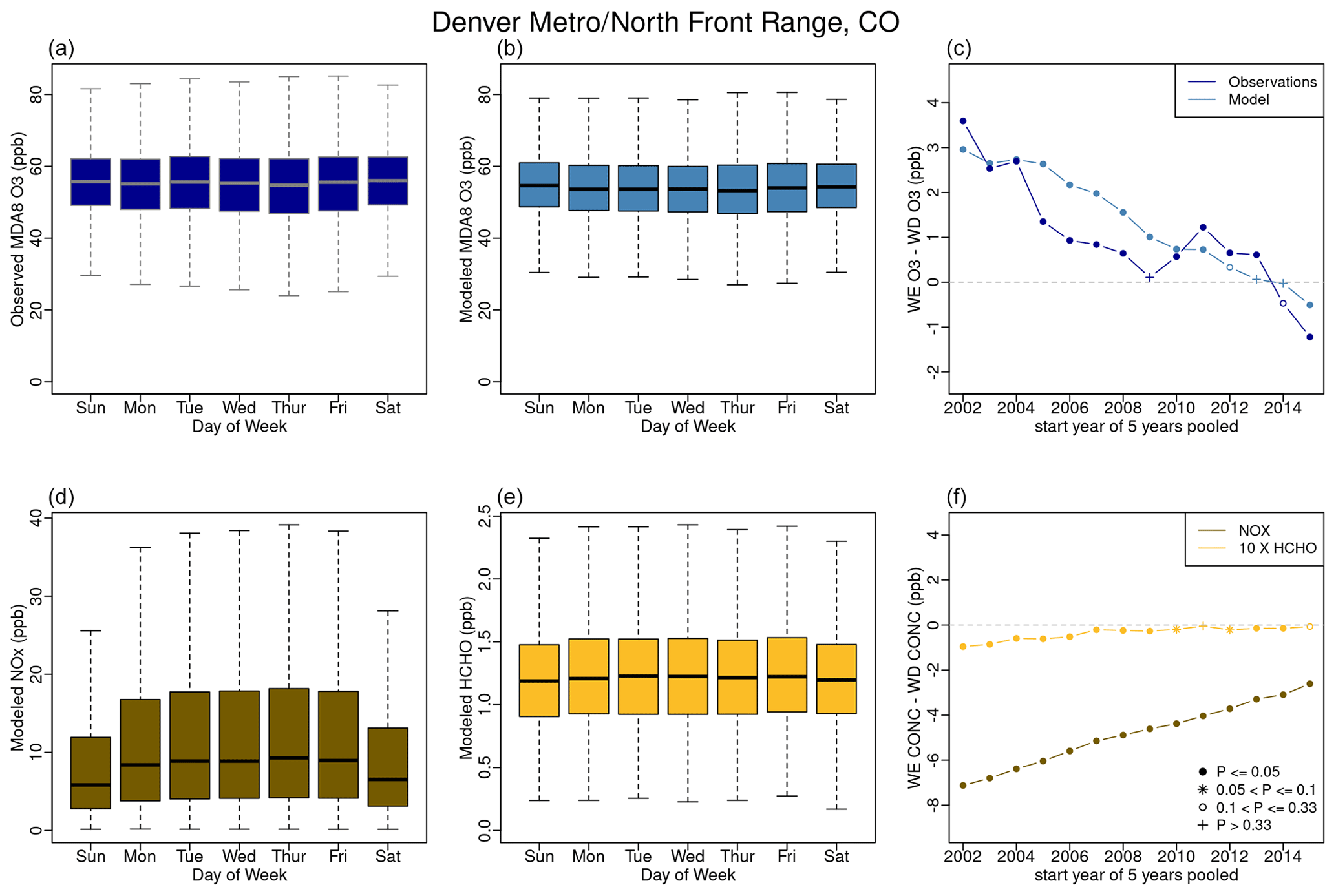
Figure 1 Denver area 2002–2019 May–September: observed (a) and modeled (b) MDA8 ozone distribution by day of week; modeled NO_x (d) and modeled formaldehyde (e) distribution by day of week; observed and modeled trends in $\mathrm{\Delta }\stackrel{\mathrm{‾}}{{\mathrm{O}}_{\mathrm{3},\mathrm{DOW}}}$ (c); and modeled trends in WE–WD NO_x and formaldehyde differences (f). The distributions by day of the week are for the entire 18 years, with each box representing the 25th to 75th percentile for that day of the week across all 18 years, the whiskers representing the 1.5 times the interquartile range, and the bold line inside the box representing the median. WE–WD differences (c, f) are based on 5-year rolling periods. P values denoted by symbols in panels (c) and (f) refer to the t test results comparing mean weekend and weekday values for each 5-year period.

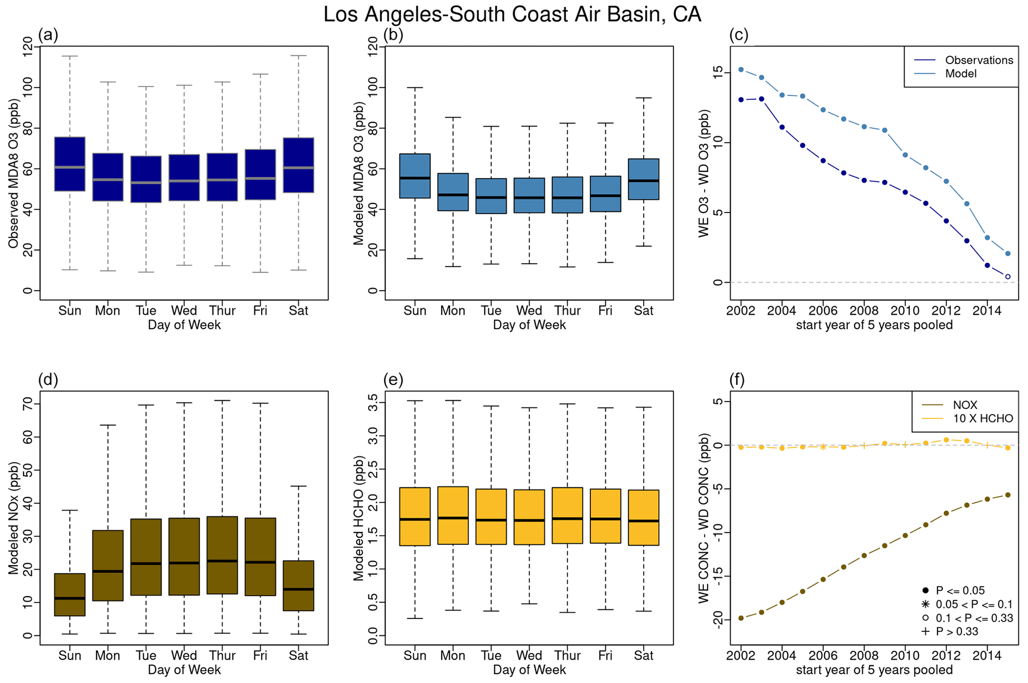
Figure 2 Los Angeles area 2002–2019 May–September: observed (a) and modeled (b) MDA8 ozone distribution by day of week; modeled NO_x (d) and modeled formaldehyde (e) distribution by day of week; observed and modeled trends in $\mathrm{\Delta }\stackrel{\mathrm{‾}}{{\mathrm{O}}_{\mathrm{3},\mathrm{DOW}}}$ (c); and modeled trends in WE–WD NO_x and formaldehyde differences (f). The distributions by day of the week are for the entire 18 years, with each box representing the 25th to 75th percentile for that day of the week across all 18 years, the whiskers representing the 1.5 times the interquartile range, and the bold line inside the box representing the median. WE–WD differences (c, f) are based on 5-year rolling periods. P values denoted by symbols in panels (c) and (f) refer to the t test results comparing mean weekend and weekday values for each 5-year period.

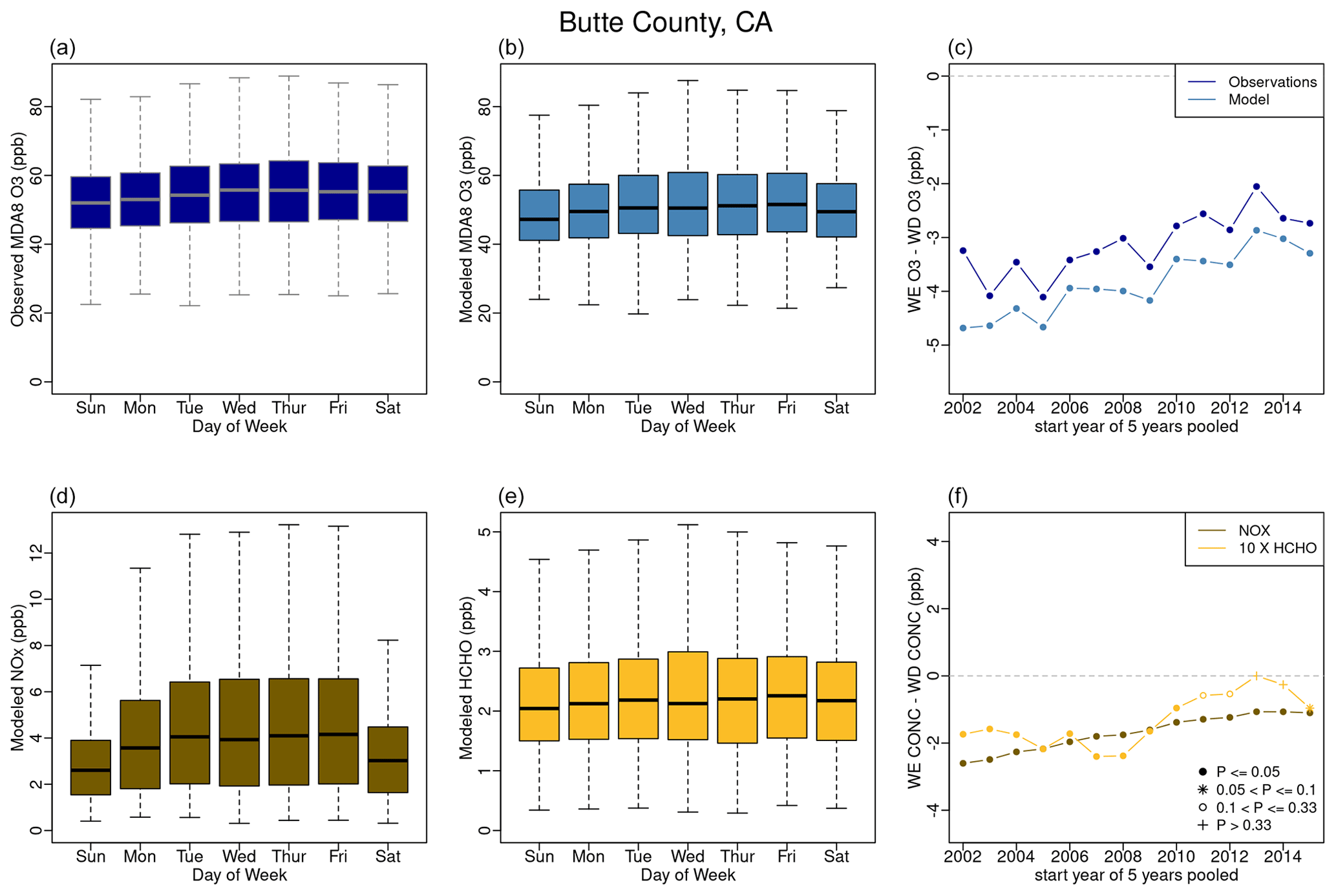
Figure 3 Butte County, CA, area 2002–2019 May–September: observed (a) and modeled (b) MDA8 ozone distribution by day of week; modeled NO_x (d) and modeled formaldehyde (e) distribution by day of week; observed and modeled trends in $\mathrm{\Delta }\stackrel{\mathrm{‾}}{{\mathrm{O}}_{\mathrm{3},\mathrm{DOW}}}$ (c); and modeled trends in WE–WD NO_x and formaldehyde differences (f). The distributions by day of the week are for the entire 18 years, with each box representing the 25th to 75th percentile for that day of the week across all 18 years, the whiskers representing the 1.5 times the interquartile range, and the bold line inside the box representing the median. WE–WD differences (c, f) are based on 5-year rolling periods. P values denoted by symbols in panels (c) and (f) refer to the t test results comparing mean weekend and weekday values for each 5-year period.

Theil–Sen trends show that differences in modeled WE versus WD NO_x have diminished over time in most areas (e.g., Figs. 1, 2, and 3). The modeled WE versus WD differences in formaldehyde are also diminishing over time but to a much lesser extent. As total emissions have decreased, absolute modeled and observed concentrations of NO_x have also decreased, along with the WE–WD differences in NO_x. Figures S33 and S34 show that the modeled WE versus WD NO_x trends remain whether tracking absolute or normalized NO_x differences in Denver and Los Angeles, which is consistent with modeled WE–WD NO_x trends seen in all but 10 of the nonattainment areas. In nine of these areas (Houston, TX; Las Vegas, NV; Muskegon, MI; New York, NY; Phoenix, AZ; San Diego, CA; St. Louis, MO–IL; Tuolumne County, CA; Yuma, AZ), absolute modeled WE–WD NO_x differences have diminished substantially, but there is little change in relative WE–WD differences. In Mariposa County, CA, neither absolute nor relative WE–WD NO_x differences have changed substantially between 2002–2019. These findings that NO_x concentrations and NO_x day-of-week patterns have decreased over time is consistent with national trends reported by Jaffe et al. (2022).

3.2 Trend types of ozone day-of-week patterns

Within any 5-year window, NO_x-saturated areas display a “weekend effect”, meaning that MDA8 ozone concentrations were higher on weekends than on weekdays, and NO_x-limited areas display a “weekday effect”, meaning that ozone concentrations were higher on weekdays than on weekends. We categorize the trends in MDA8 ozone DOW patterns into three discrete categories: (1) transitioning chemical regime (i.e., areas that went from NO_x-saturated to NO_x-limited); (2) disappearing weekday effect (i.e., areas that went from NO_x-limited to approaching zero in terms of DOW differences); and (3) areas with no trend over the 18-year time period. Transitioning chemical regime areas are characterized by a negative Theil–Sen slope (e.g., Denver and Los Angeles in Figs. 1 and 2, respectively). Disappearing weekday effect areas are characterized by a positive Theil–Sen slope (e.g., Butte County in Fig. 3). Areas with no trend are characterized by P values > 0.33 as determined by the Mann–Kendall test. Trend types for all 51 areas based on observed and modeled datasets are shown in Figs. 4 and 5. Areas are color coded by P value ranges for both the transitional chemical regime trend type and the disappearing weekday effect trend type. Given the autocorrelation of the time series data, we do not apply any strict P value thresholds for identifying these trend types, but we do note that areas with lower P values show stronger trends than those with higher P values.

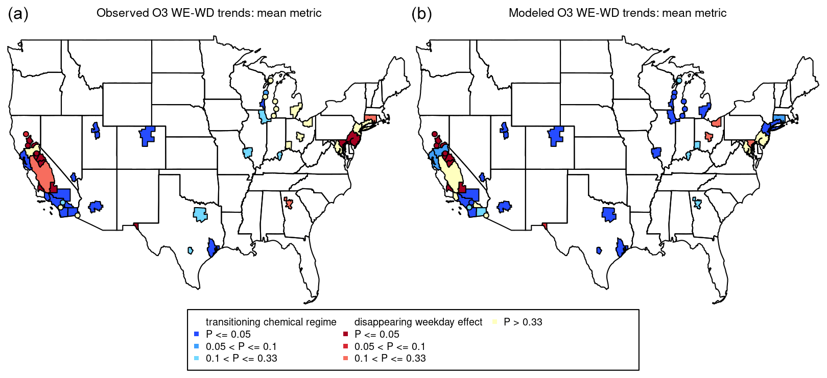
Figure 4 Map of ozone nonattainment areas color coded by trends in mean MDA8 ozone day-of-week differences ($\mathrm{\Delta }\stackrel{\mathrm{‾}}{{\mathrm{O}}_{\mathrm{3},\mathrm{DOW}}}$), using observed data (a) and modeled data (b) over an 18-year period from 2002–2019. Ozone nonattainment areas less than 3000 km² in area are shown as dots on the map for visibility.

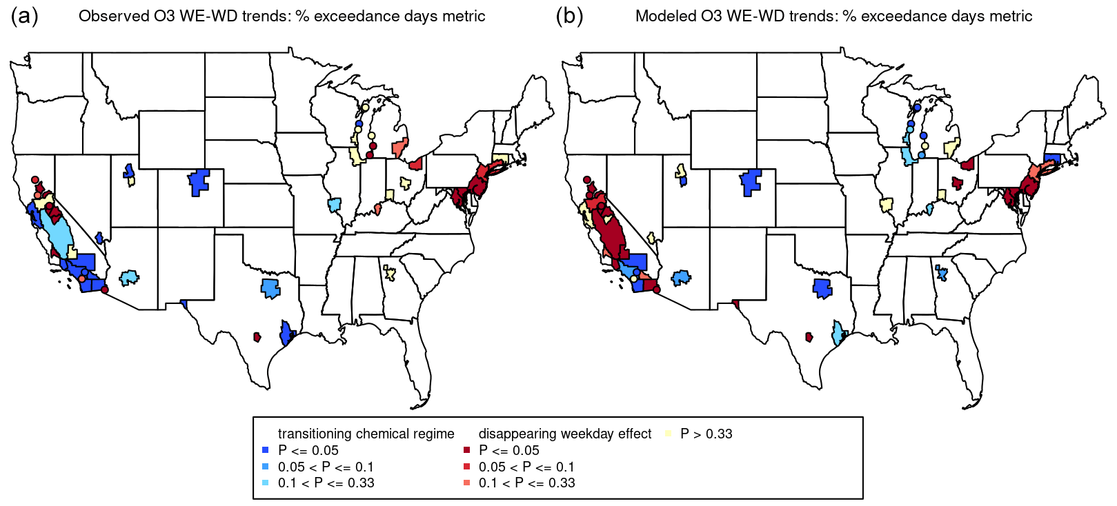
Figure 5 Map of ozone nonattainment areas color coded by trends in ozone day-of-week differences based on the percentage of days with MDA8 ozone > 70 ppb ($\mathrm{\Delta }{\mathrm{O}}_{\mathrm{3},\mathrm{DOW},\mathit{\%}>\mathrm{70}}$), using observed data (a) and modeled data (b) over an 18-year period from 2002–2019. Ozone nonattainment areas less than 3000 km² in area are shown as dots on the map for visibility.

3.2.1 Transitioning chemical regime case studies

The transitioning chemical regime trend is typical of areas that initially had strongly positive ozone WE–WD differences (i.e., mean MDA8 ozone is higher on weekends than on weekdays), suggesting NO_x-saturated conditions, at the beginning of the analysis period. These areas typically transition into near-zero or negative WE–WD MDA8 O₃ differences by the most recent 5-year window, suggesting a shift to NO_x-limited conditions by the end of the analysis period. Of the 51 nonattainment areas analyzed, 21 exhibit this type of trend for the $\mathrm{\Delta }\stackrel{\mathrm{‾}}{{\mathrm{O}}_{\mathrm{3},\mathrm{DOW}}}$ metric, based on observed data (14 with P values < 0.05; 1 with a P value between 0.05 and 0.1; 6 with P values between 0.1 and 0.33) and 31 based on modeled data (22 with P values < 0.05; 3 with P values between 0.05 and 0.1; 6 with P values between 0.1 and 0.33). Of the 51 nonattainment areas analyzed, 17 exhibit this type of trend for the $\mathrm{\Delta }{\mathrm{O}}_{\mathrm{3},\mathrm{DOW},\mathit{\%}>\mathrm{70}}$ metric, based on observed data (14 with P values < 0.05; 3 with P values between 0.1 and 0.33) and 19 based on modeled data (10 with P values < 0.05; 4 with P values between 0.05 and 0.1; 5 with P values between 0.1 and 0.33). This type of trend is consistent with previously reported national DOW trends reported across major metropolitan areas, using only the $\mathrm{\Delta }{\mathrm{O}}_{\mathrm{3},\mathrm{DOW},\mathit{\%}>\mathrm{70}}$ metric (Jaffe et al., 2022).

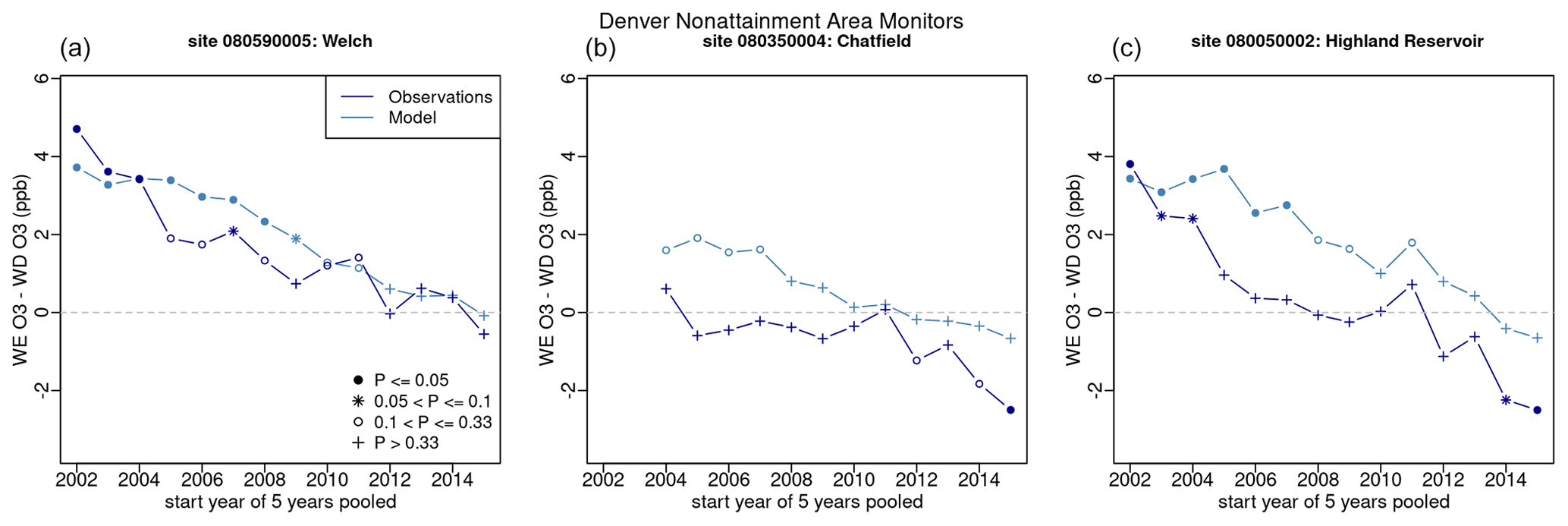
Figure 6 Observed and modeled May–September trends in mean MDA8 ozone day-of-week differences ($\mathrm{\Delta }\stackrel{\mathrm{‾}}{{\mathrm{O}}_{\mathrm{3},\mathrm{DOW}}}$) at three Denver area monitoring locations for 2002–2019 plotted as 5-year rolling periods. P values denoted by symbols refer to the t test results comparing mean weekend and weekday values for each 5-year period.

Two areas that exhibit this trend for $\mathrm{\Delta }\stackrel{\mathrm{‾}}{{\mathrm{O}}_{\mathrm{3},\mathrm{DOW}}}$ are Denver and Los Angeles, as shown in Figs. 1 and 2, respectively. Modeled and observed $\mathrm{\Delta }\stackrel{\mathrm{‾}}{{\mathrm{O}}_{\mathrm{3},\mathrm{DOW}}}$ were in the range of +3 to +4 ppb at the beginning of the analysis period for Denver. Both the observed and model data have decreasing Theil–Sen slopes for $\mathrm{\Delta }\stackrel{\mathrm{‾}}{{\mathrm{O}}_{\mathrm{3},\mathrm{DOW}}}$, −0.23 ppb yr⁻¹ (observed) and −0.29 ppb yr⁻¹ (modeled), with P values less than 0.001. In the most recent 2015–2019 5-year window, both modeled and observed $\mathrm{\Delta }\stackrel{\mathrm{‾}}{{\mathrm{O}}_{\mathrm{3},\mathrm{DOW}}}$ are negative, suggesting a shift to NO_x-limited conditions. While the results shown in Fig. 1 represent aggregated measured MDA8 ozone data across all Denver nonattainment area monitors, Fig. 6 shows behavior at three specific monitors in Denver, with monitoring records covering the majority of the analysis period. All three sites were located to the south and southwest of the Denver urban area. The Welch monitor is located closer to the Denver urban area in proximity to two major highways. While the negative observed and modeled Theil–Sen slopes for $\mathrm{\Delta }\stackrel{\mathrm{‾}}{{\mathrm{O}}_{\mathrm{3},\mathrm{DOW}}}$ hold at all three sites, there are differences in the magnitude of the slopes and the sign of $\mathrm{\Delta }\stackrel{\mathrm{‾}}{{\mathrm{O}}_{\mathrm{3},\mathrm{DOW}}}$ across sites. For instance, the Welch and Highland Reservoir sites both have positive $\mathrm{\Delta }\stackrel{\mathrm{‾}}{{\mathrm{O}}_{\mathrm{3},\mathrm{DOW}}}$ at the beginning of the analysis period, suggesting both sites were NO_x-saturated in the early 2000s. While the Chatfield site had positive $\mathrm{\Delta }\stackrel{\mathrm{‾}}{{\mathrm{O}}_{\mathrm{3},\mathrm{DOW}}}$ at the beginning of the analysis period, larger P values indicate that the differences may not be statistically different from zero, suggesting that this location may have already been transitioning to NO_x-limited conditions in the early- to mid-2000s. The model predicts that all three sites have $\mathrm{\Delta }\stackrel{\mathrm{‾}}{{\mathrm{O}}_{\mathrm{3},\mathrm{DOW}}}$ that are negative but close to zero at the end of the analysis period, while observations show the substantial negative $\mathrm{\Delta }\stackrel{\mathrm{‾}}{{\mathrm{O}}_{\mathrm{3},\mathrm{DOW}}}$ values at Chatfield and Highland Reservoir. This suggests that the model may understate the NO_x-limited conditions in recent years at these locations. Los Angeles provides another example of an area where both the model and the observations had strongly positive $\mathrm{\Delta }\stackrel{\mathrm{‾}}{{\mathrm{O}}_{\mathrm{3},\mathrm{DOW}}}$ at the beginning of the analysis period (+13 to +15 ppb) and transitioning chemical regime trends (Fig. 2) with observed and modeled Theil–Sen slopes of 0.93 and 0.83 ppb yr⁻¹. Similar to Denver, site-to-site differences in the magnitude of $\mathrm{\Delta }\stackrel{\mathrm{‾}}{{\mathrm{O}}_{\mathrm{3},\mathrm{DOW}}}$ are evident in Los Angeles (Fig. S33), but the transitioning chemical regime trend is fairly consistent across sites. Similar types of trends in Chicago and Houston are shown in Figs. S28 and S29.

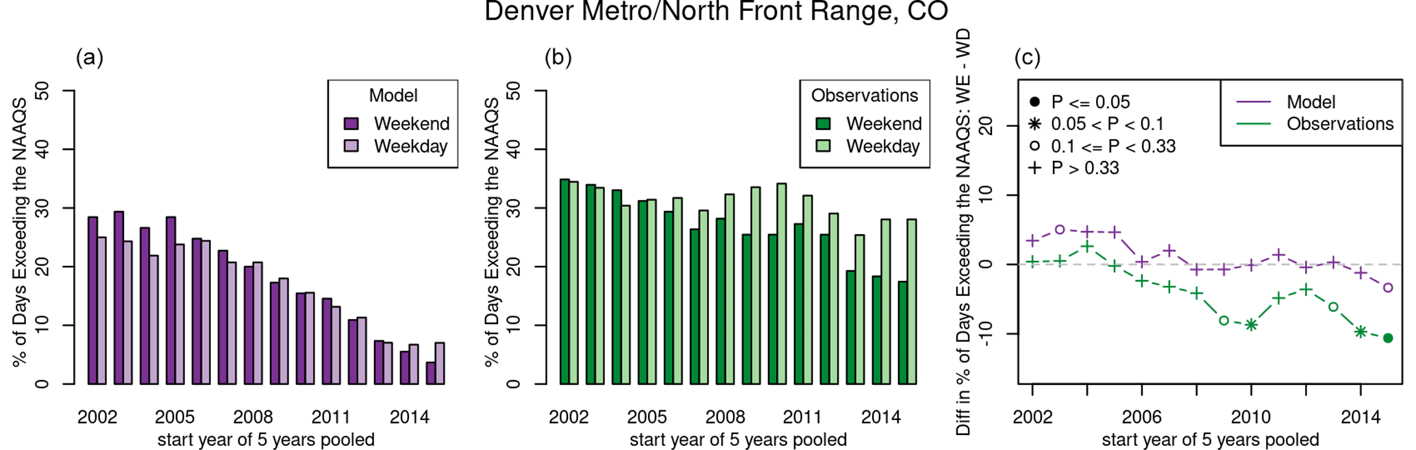
Figure 7 Modeled (a) and observed (b) percent of days with MDA8 ozone exceeding 70 ppb at any monitor within the Denver nonattainment area during May–September on weekends and weekdays for 5-year rolling periods between 2002–2019; observed and modeled trends in May–September $\mathrm{\Delta }{\mathrm{O}}_{\mathrm{3},\mathrm{DOW},\mathit{\%}>\mathrm{70}}$ at Denver area monitors for 5-year rolling periods between 2002–2019 (c). P values denoted by symbols in panel (c) refer to the t test results comparing mean weekend and weekday values for each 5-year period.

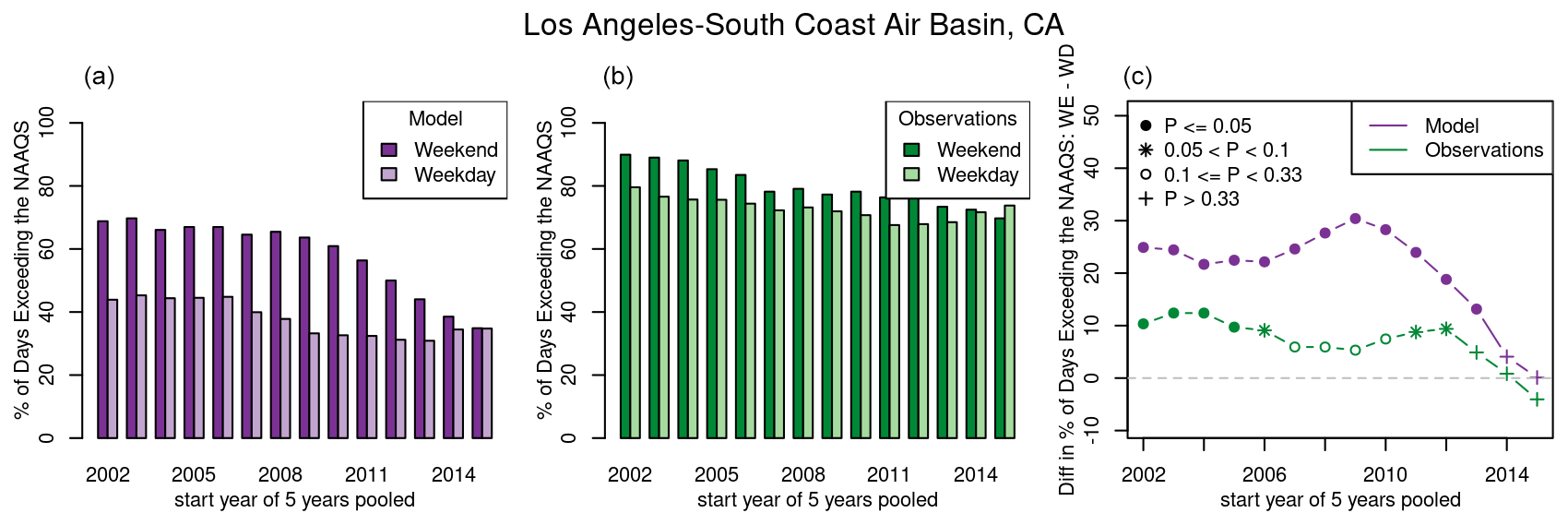
Figure 8 Modeled (a) and observed (b) percent of days with MDA8 ozone exceeding 70 ppb at any monitor within the Los Angeles nonattainment area during May–September on weekends and weekdays for 5-year rolling periods between 2002–2019; observed and modeled trends in May–September $\mathrm{\Delta }{\mathrm{O}}_{\mathrm{3},\mathrm{DOW},\mathit{\%}>\mathrm{70}}$ at Los Angeles area monitors for 5-year rolling periods between 2002–2019 (c). P values denoted by symbols in panel (c) refer to the t test results comparing mean weekend and weekday values for each 5-year period.

In general, similar transitioning chemical regime trends in $\mathrm{\Delta }{\mathrm{O}}_{\mathrm{3},\mathrm{DOW},\mathit{\%}>\mathrm{70}}$ are evident in Denver and Los Angeles (Figs. 7 and 8). In both cases, the model underpredicts both the percentage of days with MDA8 O₃ > 70 ppb and the Theil–Sen slope. Additional examples of results for $\mathrm{\Delta }{\mathrm{O}}_{\mathrm{3},\mathrm{DOW},\mathit{\%}>\mathrm{70}}$ are provided for Chicago, Houston, and New York City in Figs. S35, S36, and S37, respectively.

3.2.2 Disappearing weekday effect case study

The disappearing weekday effect trend type in the $\mathrm{\Delta }\stackrel{\mathrm{‾}}{{\mathrm{O}}_{\mathrm{3},\mathrm{DOW}}}$ metric is evident in 16 out of the 51 nonattainment areas, using observed data (12 with P values < 0.05; 1 with a P value between 0.05 and 0.1; 3 with P values between 0.1 and 0.33), and 13 out of the 51 nonattainment areas, using modeled data (9 with P values < 0.05; 1 with a P value between 0.05 and 0.1; 3 with P values between 0.1 and 0.33) (Fig. 4). Of the 51 nonattainment areas analyzed, 21 exhibit this type of trend for the $\mathrm{\Delta }{\mathrm{O}}_{\mathrm{3},\mathrm{DOW},\mathit{\%}>\mathrm{70}}$ metric based on observed data (12 with P values < 0.05; 4 with P values between 0.05 and 0.1; 5 with P values between 0.1 and 0.33) and 23 based on modeled data (17 with P values < 0.05; 1 with a P value between 0.05 and 0.1; 5 with P values between 0.1 and 0.33) (Fig. 5). This trend type is characterized by negative $\mathrm{\Delta }\stackrel{\mathrm{‾}}{{\mathrm{O}}_{\mathrm{3},\mathrm{DOW}}}$ values (i.e., weekday MDA8 ozone higher than weekend MDA8 ozone) throughout the analysis period, indicating NO_x-limited conditions trending upwards toward zero, which appears primarily in rural/agricultural areas in California. The Butte County nonattainment area in California is one example of an area exhibiting this type of day-of-week trend pattern, as is evident using both $\mathrm{\Delta }\stackrel{\mathrm{‾}}{{\mathrm{O}}_{\mathrm{3},\mathrm{DOW}}}$ and $\mathrm{\Delta }{\mathrm{O}}_{\mathrm{3},\mathrm{DOW},\mathit{\%}>\mathrm{70}}$ (Figs. 3 and 9, respectively). The disappearing weekday effect could indicate that sources without day-of-week activity patterns are becoming more dominant contributors to local NO_x emissions. In that case, the day-of-week patterns for ambient NO_x concentrations are becoming less pronounced, which would result in reductions in day-of-week MDA8 ozone patterns. An alternate explanation is that local NO_x emissions in general have decreased substantially enough that local ozone formation has become less important in such areas and a larger fraction of total ozone is being transported from upwind sources. In that case, the origin of the transported ozone could be a mixture of multiple source areas that are at varying distances upwind, which could lead to a loss in the day-of-week ozone signal. More analysis would be needed to investigate this hypothesis with respect to nonattainment areas of interest. To our knowledge, this trend type has not previously been reported in the literature, although we note some previous national assessments (i.e., Jaffe et al., 2022) did not include many of the smaller rural and agricultural areas in California where this trend is most prevalent.

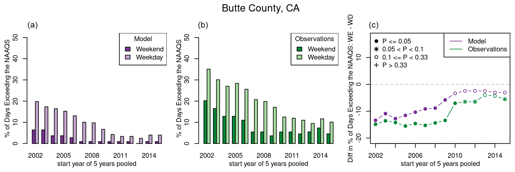
Figure 9 Modeled (a) and observed (b) percent of days with MDA8 ozone exceeding 70 ppb at any monitor within the Butte County, CA, nonattainment area during May–September on weekends and weekdays for 5-year rolling periods between 2002–2019; observed and modeled trends in May–September $\mathrm{\Delta }{\mathrm{O}}_{\mathrm{3},\mathrm{DOW},\mathit{\%}>\mathrm{70}}$ at Butte County, CA, area monitors for 5-year rolling periods between 2002–2019 (c). P values denoted by symbols in panel (c) refer to the t test results comparing mean weekend and weekday values for each 5-year period.

3.2.3 No-trend case studies

Out of the 51 nonattainment areas analyzed, 14 and 6 show no trend in the $\mathrm{\Delta }\stackrel{\mathrm{‾}}{{\mathrm{O}}_{\mathrm{3},\mathrm{DOW}}}$ metric using observed data and modeled data, respectively. Similarly, 12 and 9 show no trend in $\mathrm{\Delta }{\mathrm{O}}_{\mathrm{3},\mathrm{DOW},\mathit{\%}>\mathrm{70}}$ using observed and modeled data, respectively. The reason for the lack of trends may vary by area. Plots for several areas are provided in the Supplement. Figures S30, S34, and S37 provide the analysis for New York City, which shows no trend for the $\mathrm{\Delta }\stackrel{\mathrm{‾}}{{\mathrm{O}}_{\mathrm{3},\mathrm{DOW}}}$ using observations but instead a transitioning chemical regime trend for this metric using modeled data. Both the model and the observations show a slight increasing trend in $\mathrm{\Delta }{\mathrm{O}}_{\mathrm{3},\mathrm{DOW},\mathit{\%}>\mathrm{70}}$. One possible explanation for the lack of trends in New York is the complex nature of the emission sources and the meteorology impacting ozone formation in this area. Figure S34 shows $\mathrm{\Delta }\stackrel{\mathrm{‾}}{{\mathrm{O}}_{\mathrm{3},\mathrm{DOW}}}$ trends at three monitors in the New York City nonattainment area occurring in very different locations. The Bronx IS 52 monitor, which is located in an urbanized part of the nonattainment area, shows a transitioning chemical regime in both modeled and observed $\mathrm{\Delta }\stackrel{\mathrm{‾}}{{\mathrm{O}}_{\mathrm{3},\mathrm{DOW}}}$. In contrast, the Long Island–Riverhead monitor and the Bridgeport, CT, monitor are both located in portions of the nonattainment area that are typically downwind of the urban core on high-ozone days and are impacted by complex meteorology associated with the land–water interface near the Long Island sound. The modeled and observed data do not show substantial $\mathrm{\Delta }\stackrel{\mathrm{‾}}{{\mathrm{O}}_{\mathrm{3},\mathrm{DOW}}}$ trends at the Long Island site and only the model shows transitioning chemical regime trends at the CT site. Due to the complex nature of this large urban area, some sites may not show trends at all, and trends at other sites may be masked when aggregating data across a large number of sites.

Several nonattainment areas appear to have negative slopes in $\mathrm{\Delta }\stackrel{\mathrm{‾}}{{\mathrm{O}}_{\mathrm{3},\mathrm{DOW}}}$ at the beginning of the analysis period and positive slopes at the end of the analysis period, resulting in no overall trend over the entire period. Cincinnati, OH–KY, exemplifies this pattern, and on closer inspection, the patterns appear to mirror annual changes in WE–WD patterns in multiple meteorological parameters (Fig. S38). For Cincinnati, the correlation coefficients between WE–WD MDA8 O₃ differences and WE–WD meteorological parameter differences were 0.77, −0.83, 0.79, 0.89, −0.94, and −0.73 for daily maximum temperature, daily average relative humidity, daily maximum planetary boundary layer height, solar radiation, percent cloud cover, and 24 h transport direction, respectively. Other areas exhibiting this behavior are all located in relatively close proximity to Cincinnati, including Louisville, KY–IN, and St. Louis, MO–IL, and to a lesser extent Columbus, OH, and Atlanta, GA. These findings suggest that for these areas even 5-year processing blocks may not be sufficient to remove the effects of spurious weekly meteorological variations on ozone. Figure S39 shows that the correlation between WE–WD differences in seven meteorological variables, and observed $\mathrm{\Delta }\stackrel{\mathrm{‾}}{{\mathrm{O}}_{\mathrm{3},\mathrm{DOW}}}$ do not appear to be a driving factor in significant $\mathrm{\Delta }\stackrel{\mathrm{‾}}{{\mathrm{O}}_{\mathrm{3},\mathrm{DOW}}}$ trends in other areas, but it is possible that some additional areas which do not have trends in $\mathrm{\Delta }\stackrel{\mathrm{‾}}{{\mathrm{O}}_{\mathrm{3},\mathrm{DOW}}}$ may also be impacted by meteorological variations.

3.3 Comparison of modeled and observed trends in ozone day-of-week patterns

The modeled and observed trends in WE–WD differences for each of the 51 nonattainment areas are provided in Table S1 ($\mathrm{\Delta }\stackrel{\mathrm{‾}}{{\mathrm{O}}_{\mathrm{3},\mathrm{DOW}}}$) and Table S2 ($\mathrm{\Delta }{\mathrm{O}}_{\mathrm{3},\mathrm{DOW},\mathit{\%}>\mathrm{70}}$). Figure 10 provides a comparison of modeled to observed WE–WD differences across the 51 nonattainment areas at the beginning of the analysis period (2002–2006) and at the end of the analysis period (2015–2019). Each point represents the WE–WD MDA8 ozone difference for a single nonattainment area, with the left-hand panel showing $\mathrm{\Delta }\stackrel{\mathrm{‾}}{{\mathrm{O}}_{\mathrm{3},\mathrm{DOW}}}$ and the right-hand panel showing $\mathrm{\Delta }{\mathrm{O}}_{\mathrm{3},\mathrm{DOW},\mathit{\%}>\mathrm{70}}$. Data points falling in the upper-right quadrant of each panel represent areas for which both the observations and the modeled DOW patterns suggest NO_x-saturated conditions. Data points in the lower-left quadrant of each panel represent areas for which both the observations and the model DOW patterns suggest NO_x-limited conditions. In the earlier 2002–2006 time period, there are a large number of areas falling in both the upper-right and lower-left quadrants for both metrics. In the 2015–2019 time period, almost all areas are located in the lower-left quadrant for both metrics, suggesting that most USA nonattainment areas have transitioned into NO_x-limited conditions. The correlation of modeled and observed WE–WD differences is quite high (r = 0.94 and 0.82 for $\mathrm{\Delta }\stackrel{\mathrm{‾}}{{\mathrm{O}}_{\mathrm{3},\mathrm{DOW}}}$ in the earliest and most recent time periods, respectively; r = 0.7 and 0.62 for $\mathrm{\Delta }{\mathrm{O}}_{\mathrm{3},\mathrm{DOW},\mathit{\%}>\mathrm{70}}$ in the earliest and most recent time periods, respectively). For both metrics, the majority of points fall above the 1 : 1 line, indicating that, in general, the model overestimated the degree of NO_x-saturated conditions and underestimated the degree of NO_x-limited conditions.

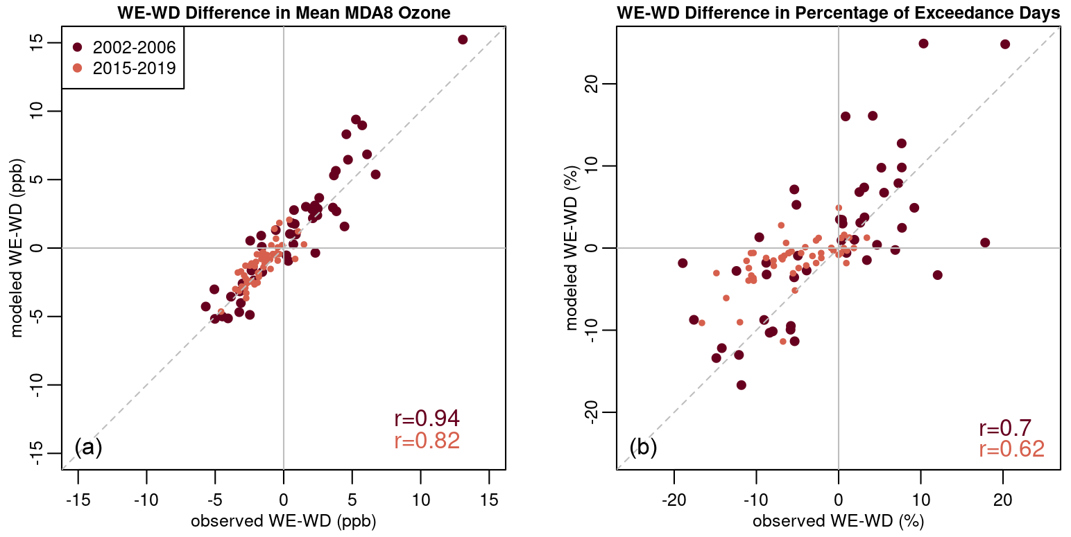
Figure 10 Comparison of modeled and observed WE–WD MDA8 O₃ differences for $\mathrm{\Delta }\stackrel{\mathrm{‾}}{{\mathrm{O}}_{\mathrm{3},\mathrm{DOW}}}$ (a) and $\mathrm{\Delta }{\mathrm{O}}_{\mathrm{3},\mathrm{DOW},\mathit{\%}>\mathrm{70}}$ (b). Differences shown for the 2002–2006 time period and for the 2015–2019 time period. Each dot represents a different nonattainment area.

Maps in Figs. 4 and 5 show the locations of areas predicted to have transitioning chemical regime trends, disappearing weekday effect trends, and no trends for $\mathrm{\Delta }\stackrel{\mathrm{‾}}{{\mathrm{O}}_{\mathrm{3},\mathrm{DOW}}}$ and $\mathrm{\Delta }{\mathrm{O}}_{\mathrm{3},\mathrm{DOW},\mathit{\%}>\mathrm{70}}$, respectively. The maps show general consistency among which areas are predicted to have each trend type between observations and the model. Nine areas are predicted to have transitioning chemical regime trends with P values < 0.05 in both datasets and with both metrics indicating strong agreement that they are shifting to more NO_x-limited conditions (Milwaukee, WI; Houston, TX; Phoenix, AZ; Denver, CO; Northern Wasatch Front, UT; Southern Wasatch Front, UT; Las Vegas, NV; Los Angeles – San Bernardino County, CA; Los Angeles – South Coast, CA; and San Diego, CA).

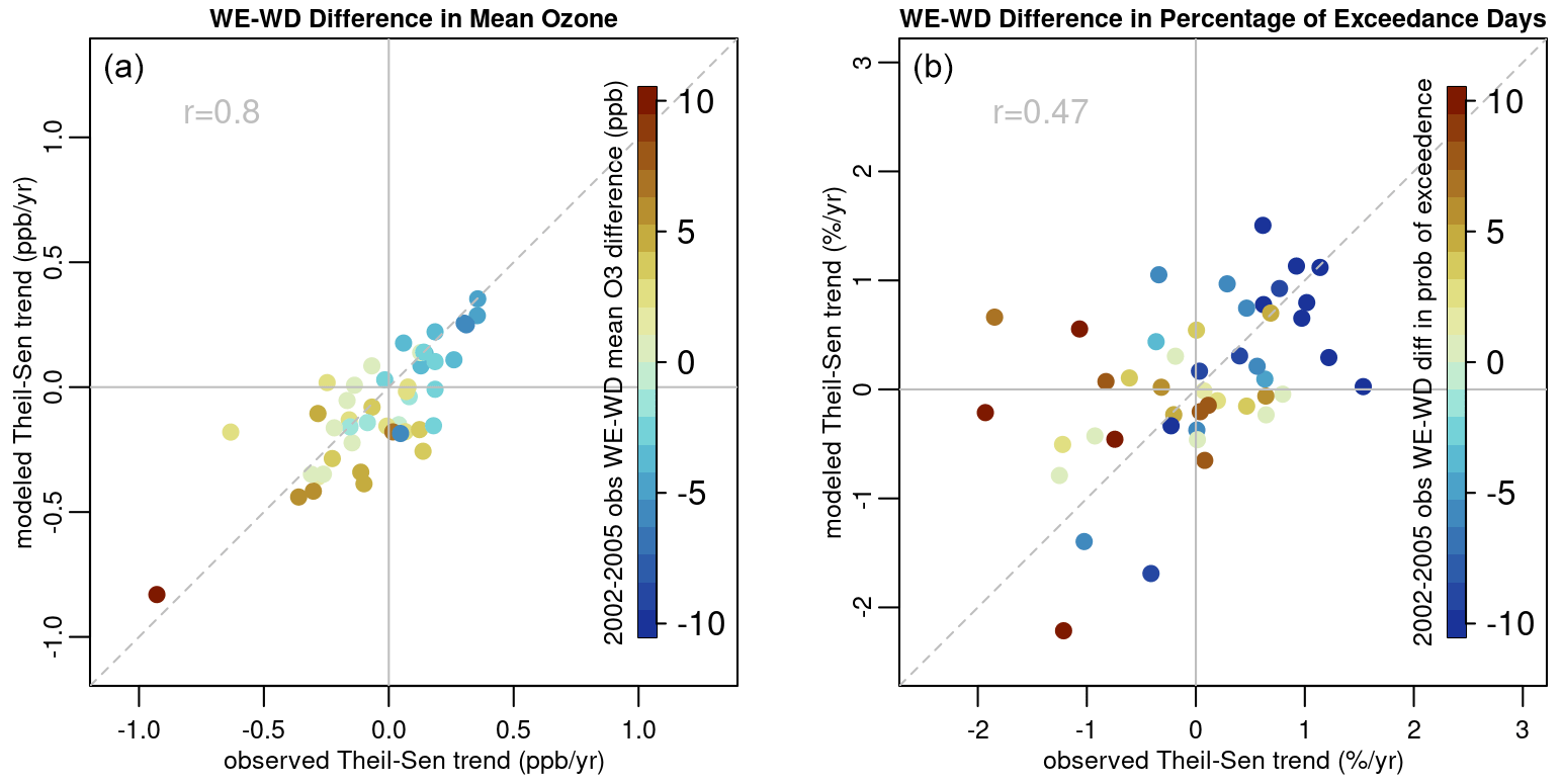
Figure 11 Comparison of modeled and observed Theil–Sen slopes in May–September WE–WD MDA8 O₃ differences across all nonattainment areas for $\mathrm{\Delta }\stackrel{\mathrm{‾}}{{\mathrm{O}}_{\mathrm{3},\mathrm{DOW}}}$ (a) and $\mathrm{\Delta }{\mathrm{O}}_{\mathrm{3},\mathrm{DOW},\mathit{\%}>\mathrm{70}}$ (b). WE–WD differences for the 2002–2005 time-period are indicated by the color bar, with positive differences (NO_x-saturated areas) shown in shades of yellow and brown and negative differences (NO_x-limited areas) shown in shades of blue. Note that the brown symbol at the bottom left of both panels represents the Los Angeles nonattainment area.

Figure 11 compares modeled and observed Theil–Sen slopes in WE–WD MDA8 O₃ differences across all areas. Each point represents a single nonattainment area color coded by 2002–2005 $\mathrm{\Delta }\stackrel{\mathrm{‾}}{{\mathrm{O}}_{\mathrm{3},\mathrm{DOW}}}$ or $\mathrm{\Delta }{\mathrm{O}}_{\mathrm{3},\mathrm{DOW},\mathit{\%}>\mathrm{70}}$. The correlation of modeled versus observed Theil–Sen slopes using $\mathrm{\Delta }\stackrel{\mathrm{‾}}{{\mathrm{O}}_{\mathrm{3},\mathrm{DOW}}}$ is stronger (r = 0.8) than the correlation using $\mathrm{\Delta }{\mathrm{O}}_{\mathrm{3},\mathrm{DOW},\mathit{\%}>\mathrm{70}}$ (r = 0.47). While the model does not always correctly predict the Theil–Sen slope, the data fall close to the 1 : 1 line for the $\mathrm{\Delta }\stackrel{\mathrm{‾}}{{\mathrm{O}}_{\mathrm{3},\mathrm{DOW}}}$, suggesting that the model does not systematically over- or underpredict the trends in WE–WD differences from 2002–2019. The trend types described above for $\mathrm{\Delta }\stackrel{\mathrm{‾}}{{\mathrm{O}}_{\mathrm{3},\mathrm{DOW}}}$ metric are visible in the left panel of Fig. 11. Most NO_x-saturated areas (yellow and brown symbols) and some NO_x-limited areas (blue symbols) have negative Theil–Sen slopes (i.e., transitioning chemical regime) towards NO_x-limited conditions similar to those described above for Denver and Los Angeles (shown as the dark brown symbol at the bottom left of the plot). Areas with positive Theil–Sen slopes tend to be the most NO_x-limited areas (darker blue symbols) and represent the disappearing weekday trends demonstrated by Butte County. The model is not as accurate at predicting $\mathrm{\Delta }{\mathrm{O}}_{\mathrm{3},\mathrm{DOW},\mathit{\%}>\mathrm{70}}$ Theil–Sen slopes as $\mathrm{\Delta }\stackrel{\mathrm{‾}}{{\mathrm{O}}_{\mathrm{3},\mathrm{DOW}}}$ Theil–Sen slopes, as evidenced by the increased scatter in the right-hand panel of Fig. 11 compared to the left-hand panel. Some areas have few exceedances of the NAAQS in the later years of the trends period, and this small sample size could explain the difference between the monitored and modeled slopes, given that the model predicted fewer exceedance days than were observed in many areas.

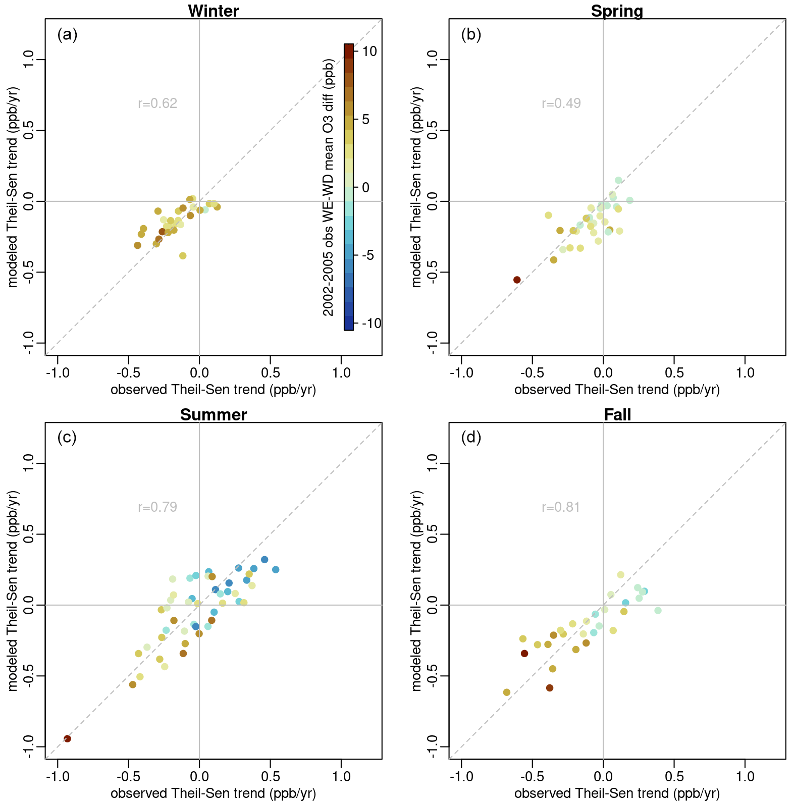
Figure 12 Comparison of modeled and observed $\mathrm{\Delta }\stackrel{\mathrm{‾}}{{\mathrm{O}}_{\mathrm{3},\mathrm{DOW}}}$ Theil–Sen slopes across all nonattainment areas in winter (a), spring (b), summer (c), and fall (d). WE–WD differences for the 2002–2005 time-period are indicated by the color bar, with positive differences (NO_x-saturated areas) shown in shades of yellow and brown and negative differences (NO_x-limited areas) shown in shades of blue. Note that year-round ozone monitoring is not required in some parts of the USA, and therefore monitoring data may not be available outside the May–September period in some areas.

Figure 12 shows the comparison of $\mathrm{\Delta }\stackrel{\mathrm{‾}}{{\mathrm{O}}_{\mathrm{3},\mathrm{DOW}}}$ Theil–Sen slopes by season. The summer plot looks similar to the May–September plot shown in Fig. 11. Winter, spring, and fall data show median $\mathrm{\Delta }\stackrel{\mathrm{‾}}{{\mathrm{O}}_{\mathrm{3},\mathrm{DOW}}}$ near zero or greater than zero in most nonattainment areas, suggesting transitional or NO_x-saturated conditions in these seasons. Both observations and model predictions suggest $\mathrm{\Delta }\stackrel{\mathrm{‾}}{{\mathrm{O}}_{\mathrm{3},\mathrm{DOW}}}$ negative Theil–Sen slopes in these seasons, suggesting that nonattainment areas in the USA may be transitioning towards NO_x-limited conditions even outside of the summer ozone season.

4 Conclusions

While this assessment has provided insight into the ozone formation regimes across high-ozone locations in the USA, some key questions remain about the important drivers for year-to-year changes in DOW MDA8 ozone patterns and which of those drivers are well captured by the EQUATES dataset. First, while NO_x and VOC emissions have been steadily decreasing across most areas of the USA, exceptions to that pattern include increasing wildfire emissions, especially in the western USA, and increasing emissions from oil and gas activities near USA nonattainment areas in Texas, Colorado, New Mexico, and Utah. Future work could focus on areas impacted by these two emission sources to assess both the impact of these increasing emissions on ozone formation regimes and the ability of the EQUATES dataset to capture those impacts. Second, this assessment predominantly focused on MDA8 ozone values across the May–September ozone season; however, past work has identified some seasonally varying ozone biases within the CMAQ model (Appel et al., 2021). Specifically, EQUATES has a tendency to underpredict ozone during the spring and overpredict ozone later in the summer (Figs. S40 and S41). Given that ozone formation tends to be more NO_x-saturated in the springtime than in the summer (Jin et al., 2020, 2017), a more in-depth assessment would be needed to fully characterize the extent that differences in observed and modeled WE–WD MDA8 ozone differences are impacted by this seasonally varying model performance. Third, we assessed DOW MDA8 ozone patterns across multiple complex urban areas that encompassed spatially heterogeneous emission sources and meteorology. For some of these areas (e.g., Los Angeles, CA, and Denver, CO) the sign of the Theil–Sen slopes in WE–WD MDA8 ozone appeared consistent across monitoring locations, while in others (e.g., New York City, NY) different monitoring locations across the area appeared to show different types of trends. Further local-scale investigation into each of these areas would be necessary to fully characterize the nuances of DOW and year-to-year variations in emission and meteorology that obscure the MDA8 ozone DOW trends in some areas but not others when aggregating across monitor locations in those areas. Finally, an intriguing trend in MDA8 ozone DOW patterns was identified in multiple rural and agricultural areas of California. Recent literature has suggested that soil NO emissions, which are unlikely to have a DOW emission pattern, are an important NO_x emission source in agricultural locations of California (Almaraz et al., 2018; Zhu et al., 2023). Could the MDA8 ozone DOW trends observed in these areas be reflective of the increasing relative importance of NO_x sources other than mobile sources in those locations? More assessment is needed to definitively determine whether the trend in a decreasing weekday effect is a reliable indicator of areas that are becoming more dominated by local NO_x sources that do not vary by DOW, more dominated by transported ozone, or some other factor. It is important to note that transported ozone may come from nearby regional sources or from longer range sources provided the transport times are sufficient to mask any DOW patterns that would be evident in the source region.

In this analysis, we found that trends in ozone formation chemistry may not always be clearly shown by trends in DOW patterns, which are impacted by a complex set of local factors including meteorology, the mix of local emission sources, and monitor locations in relationship to land–water interfaces. Lack of trends appear more often, using observed data than modeled data (Figs. 4 and 5), meaning that, while the model accurately captures Theil–Sen slopes for $\mathrm{\Delta }\stackrel{\mathrm{‾}}{{\mathrm{O}}_{\mathrm{3},\mathrm{DOW}}}$ and $\mathrm{\Delta }{\mathrm{O}}_{\mathrm{3},\mathrm{DOW},\mathit{\%}>\mathrm{70}}$ (Fig. 11), lower P values are less common when using observational data. This suggests that there may be some stochastic processes making observed year-to-year WE–WD MDA8 ozone differences noisy, which are not fully captured by the model. Even with these limitations, this analysis has shown that DOW patterns in ambient NO_x concentrations persist in USA urban areas but have become less prominent in some areas, while others have transitioned from positive WE–WD MDA8 ozone differences to negative WE–WD MDA8 ozone differences over the 18-year period analyzed. These DOW NO_x differences have resulted in distinctive DOW MDA8 ozone patterns in many of the nonattainment areas assessed. The EQUATES modeling simulations appear to show larger and more positive WE–WD MDA8 ozone differences than observational data, suggesting that ozone formation in this modeling dataset is less NO_x-limited than in the observations. Despite this discrepancy, the EQUATES dataset captures year-to-year changes in WE–WD MDA8 ozone patterns, as demonstrated by high correlation of the Theil–Sen slopes for WE–WD MDA8 ozone differences. The agreement between the modeled and observation datasets is more apparent when assessing summertime mean MDA8 ozone than when analyzing extreme values using the percentage of exceedance days metric. Assessing frequencies or magnitudes of extreme values is challenging when using a dataset with a limited number of weekend and weekday days, due to the stochastic and infrequent nature of high-ozone events in many areas.

While there are multiple types of measurements and modeling assessments that can be applied to characterize local ozone formation regimes, many of these require specialized measurements or datasets that are not readily available in all areas. In contrast, assessing DOW MDA8 ozone patterns requires only routine daily ozone measurements that are widely available across urban areas in the USA and in other countries. Consequently, this type of assessment is a useful tool and may be applied in many areas using routine measurements. In locations with long-term measurements, DOW patterns offer a method to look at trends in ozone formation chemistry over time. While DOW patterns in MDA8 ozone are especially useful, given the wide availability of data required for this type of assessment, we anticipate that in the near future, additional datasets for assessing ozone chemical formation regimes will become more widely available. Specifically, O3, NO2, and HCHO data from the recently launched Tropospheric Emissions: Monitoring of POllution (TEMPO) satellite may provide the ability to better understand the relationships between WE–WD MDA8 ozone patterns and precursor concentrations.