Technical note: Accurate, reliable, and high-resolution air quality predictions by improving the Copernicus Atmosphere Monitoring Service using a novel statistical post-processing method

Starting from the regional air quality forecasts produced by the Copernicus Atmosphere Monitoring Service (CAMS), we propose a novel post-processing approach to improve and downscale results on a finer scale. Our approach is based on the combination of ensemble model output statistics (EMOS) with a spatio-temporal interpolation process performed through the stochastic partial differential equation–integrated nested laplace approximation (SPDE-INLA). Our interpolation approach includes several spatial and spatio-temporal predictors, including meteorological variables. A use case is provided that scales down the CAMS forecasts on the Italian peninsula. The calibration is focused on the concentrations of several air quality pollutants (PM₁₀, PM_2.5, NO₂, and O₃) at a daily resolution from a set of 750 monitoring sites, distributed throughout the Italian country. Our results show the key role that conditioning variables play in improving the forecast capabilities of ensemble predictions, thus allowing for a net improvement in the calibration with respect to ordinary EMOS strategies. From a deterministic point of view, the performance of the predictive model shows a significant improvement in the performance of the raw ensemble forecast, with an almost-zero bias, significantly reduced root mean square errors, and correlations that are almost always higher than 0.9 for each pollutant; moreover, the post-processing approach is able to significantly improve the prediction of exceedances, even for very low thresholds, such as those recently recommended by the World Health Organisation. This is particularly significant if a forecasting approach is used to predict air quality conditions and plan adequate human health protection measures, even for low alert thresholds. From a probabilistic point of view, the quality of the forecast was verified in terms of reliability and credible intervals. After post-processing, the predictive probability density functions were sharp and much better calibrated than the raw ensemble forecast. Finally, we present some additional results based on a set of gridded (4 km × 4 km) maps covering the entire Italian country for the detection of areas where pollution peaks occur (exceedances of the current and/or proposed regulatory thresholds).

1 Introduction

Outdoor air pollution induced by natural sources and human activities remains a major environmental problem of concern worldwide. Studies have shown that particulate matter, ozone, and nitrogen dioxide degrade ambient air quality and cause serious health problems to human beings (Kim et al., 2015; Kampa and Castanas, 2008; Manisalidis et al., 2020). For example, recent studies have suggested that air pollution, particularly traffic-related pollution, is associated with pre-term birth and infant mortality and the development of asthma and atopy (Khreis et al., 2017; Burbank and Peden, 2018). A joint study of the World Bank and the Institute for Health Metrics and Evaluation (World Bank, 2016) has shown how air pollution also has huge implications for world economies: approximately 5.5 million lives were lost in 2013 from diseases associated with outdoor and indoor air pollution, with the global economic cost of those deaths being approximately USD 225 billion in lost labour income and over USD 5 trillion in welfare losses.

Producing reliable short-term forecasts of pollutant concentrations is a key challenge in supporting national authorities in their tasks related to EU Air Quality Directives, such as planning and reporting the state of air quality to citizens. Starting in 2014, the Copernicus Atmosphere Monitoring Service (CAMS), a service implemented by the European Centre for Medium-Range Weather Forecasts (ECMWF), has continuously provided air quality forecasts throughout Europe, supporting this task. This system is based on an ensemble of several models (Marécal et al., 2015). The different individual model results are interpolated on a common regular 0.1^∘ × 0.1^∘ grid over the European domain (30–72^∘ N, 25^∘ W–45^∘ E) for the next 4 d at an hourly time resolution, and a median ENSEMBLE is calculated from the model output.

Higher spatial resolutions are achieved through smaller-scale applications, such as those used for the FORAIR-IT (Mircea et al., 2014), kAIROS (Stortini et al., 2020), PREV'AIR (Rouil et al., 2009), UK-AIR (DEFRA, 2022), or CALIOPE (Baldasano et al., 2008) systems. However, all these systems require the use of more detailed information and obviously imply the use of much greater computational resources. On the other hand, the use of raw CAMS forecasts do not permit the reproduction of subgrid-scale features, especially close to large point emission sources. There is a reasonable expectation that even the ENSEMBLE results have limited skill under complex local-scale conditions, with expected ensemble mean and variance correlated with the observations and the actual model uncertainty, respectively, and a persistent underestimation of the true observations and model uncertainty.

However, understanding how well pollutant concentrations can be predicted in both space and time is essential for a proper assessment of warning and alarm levels and to capture concentration gradients even at high spatial resolutions (Buizza et al., 2022; Chianese et al., 2018; Cohen et al., 2017; Lindström et al., 2014; Zhou et al., 2019). In recent years, there has been an increasing interest in spatio-temporal statistical models, which combine ensemble predictions, data assimilation, and machine learning, and these models have quickly gained attention in the air quality scientific community (Bai et al., 2018; Zhang et al., 2012). The reason lies in the fact that hybrid models are easier to implement and do not require high computational resources, while deterministic models are often more computationally expensive and difficult to manage in terms of quality and the number of input data requests (Bertrand et al., 2023; Camastra et al., 2022; Chianese et al., 2019; Taheri Shahraiyni and Sodoudi, 2016).

In this study, starting from the CAMS air quality forecasts, we studied the possibility of improving the 24 h evolution of PM₁₀, PM_2.5 (daily averages), O₃ (highest 8 h daily maximum), and NO₂ (1 h daily maximum) in Italy. This country is characterised by complex conditions for modelling air pollution due to topographic characteristics, different geoclimatic zones, and the complex mix of anthropogenic and natural sources of air pollution. Thus, post-processing of CAMS raw ensemble results may be particularly suitable for such areas, where the results of the different models could benefit from the use of additional information for a more accurate and higher-resolution estimation.

In this work, a post-processing framework was used to improve the estimation of the air quality forecast in Italy, combining the deterministic forecasts with additional spatio-temporal predictors within a statistical framework. More precisely, we designed an output statistical framework for the output data from CAMS models to obtain a well-calibrated and bias-corrected ensemble prediction and then fit this calibrated ensemble prediction within a spatio-temporal hierarchical model using the integrated nested Laplace approximation stochastic partial differential equation (INLA-SPDE) approach. The INLA-SPDE method is a deterministic approach to Bayesian inference, as opposed to the Markov chain Monte Carlo (MCMC) method, a simulation-based approach (Gilks et al., 1995; Riccio et al., 2006), for which computational costs are very demanding. Conversely, the INLA-SPDE method has been shown to provide a viable method to speed up calculations, even for large-scale problems, without sacrificing accuracy (Rue et al., 2009).

The remainder of this paper is organised as follows. In Sect. 2, we first introduce the input data set chosen to analyse pollutant concentrations, and in Sect. 3, we outline the methods used to develop the post-processing approach. Next, Sect. 4 discusses the results, model validation, and two possible applications of the model estimates for predicting threshold levels in Italy. Conclusions are reported in Sect. 5.

2 Data

2.1 The CAMS suite

CAMS provides daily analyses and forecasts of long-range transport of atmospheric pollutants around the world, as well as air quality forecasts for the European domain, updated on a daily basis. On a global scale, CAMS provides 5 d forecasts for aerosols, atmospheric pollutants, greenhouse gases, and stratospheric ozone and UV index. On the European scale, predictions are issued with a resolution of 0.1^∘ × 0.1^∘ over Europe and 10 vertical levels from the Earth surface up to 5000 m, combining data with satellite and non-satellite observations.

The CAMS ensemble prediction system started with a suite composed of seven air quality models: CHIMERE, EMEP, EURAD-IM, LOTOS-EUROS, MATCH, MOCAGE, and SILAM. At the end of 2019, the DEHM (Aarhus University, Denmark) and GEM-AQ (IEP-NRI, Poland) models were added. From June 2022, two additional models (MINNI, operated by ENEA, Italy, and the Barcelona Supercomputing Centre's MONARCH model) have delivered their results, as well as expanding the ensemble size to 11 members. The 00:00 UTC ECMWF-IFS (Integrated Forecast System) provides the meteorological data for the prediction of transport phenomena, and the CAMS emission database provides the input data for the simulation of emission phenomena. CAMS forecasts are available for download from the CAMS Atmosphere Data Store. The full range of forecasts is guaranteed to be available by 08:00 UTC every day for the next 4 d. Marécal et al. (2015) provide the full details on the implementation of this multi-model forecast system.

2.2 Training data and predictors

Our ultimate goal is to improve the CAMS forecast on the Italian peninsula. This geographic area is characterised by complex orographic and climatic conditions, including the mountain systems of the Alpine arc (to the north) and Apennines (along the entire longitudinal ridge from north to south), an extensive flat area (the Po Valley), and two major islands (Sicily and Sardinia). Furthermore, the transport of desert dust in the Mediterranean region often affects the concentration of PM, with a significant impact on the health of the population (Alahmad et al., 2023; Sajani et al., 2011). This variety of orographic and climatic conditions leads to a high spatial variability of air quality conditions, which makes the Italian peninsula a significant test bed for the predictive capabilities of the CAMS ensemble.

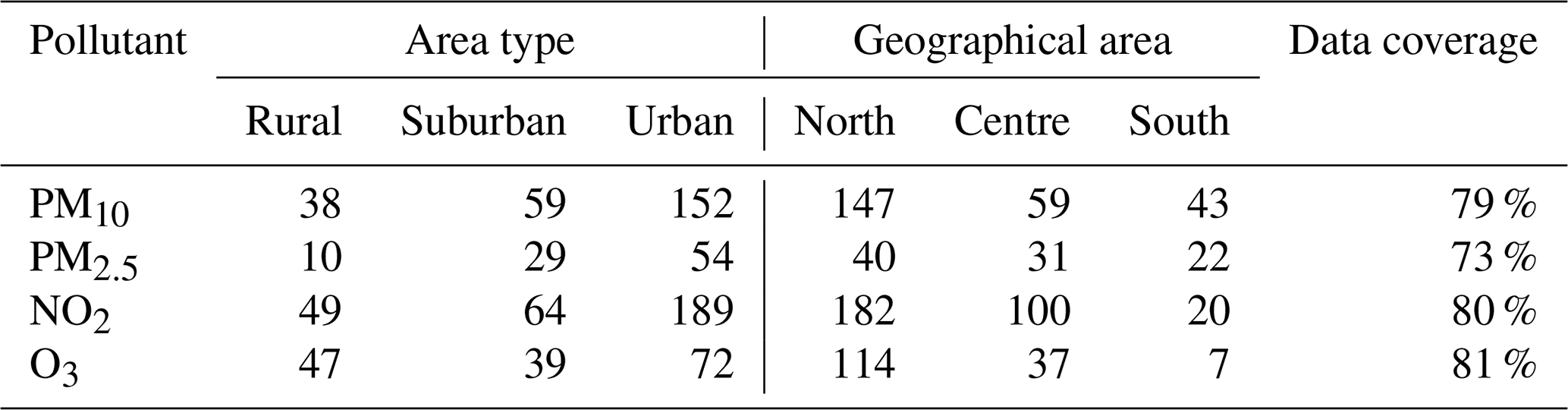
In the present study, the following air quality pollutants have been considered: PM₁₀ and PM_2.5 (daily averages), O₃ (highest 8 h daily maximum), and NO₂ (1 h daily maximum). Table 1 reports the number of ground stations for each of the pollutants measured together with the type of area, the geographic area, and the data coverage (defined as the average percentage of valid data at all monitoring stations for the year 2022). These data are available from the up-to-date (UTD) channel of the Air Quality E-reporting system (https://www.eea.europa.eu/data-and-maps/data/aqereporting-9, last access: 25 November 2023) of the European Environment Agency (EEA), from which they can be freely downloaded.

According to the information communicated to the EEA, the Italian air quality network is made up of a total of 750 monitoring stations, unevenly distributed by area type: most of the monitoring stations are clustered around urban areas, while remote or rural areas are less represented. These monitoring stations are also unevenly distributed with respect to altitude, with most monitoring sites below 250 m. This is not surprising at all since most of the stations are located where high concentrations are expected, that is, at low-altitude urban or suburban sites. Furthermore, these stations are not evenly distributed with respect to geographic area, with most of the stations located in northern regions and, to a lesser extent, in central and southern Italy.

Table 1 Details of observation stations with at least 90 % of valid data for the year 2022 grouped by pollutant, geographical area, and area type. Data coverage refers to the average percentage of valid data over all monitoring stations.

As complementary information to the concentration of the main trace pollutants, several geographic and/or meteorological variables may have a potentially predictive role for air quality. The use of spatio-temporal predictors is by no means uncommon in air quality modelling as they are usually exploited to capture the high-frequency variability at finer spatial scales (Bertrand et al., 2023; Shtein et al., 2019; Stafoggia et al., 2020). The predictors used in this study can be classified into two different categories: (1) purely spatial predictors and (2) spatio-temporal predictors. The first category includes all geographic variables that do not have a variable temporal component, while the second category may vary over time. For each monitoring station, we first built a circular buffer with a radius of 5000 m, comparable to the resolution of the raw CAMS predictions, and sampled the density of each purely spatial predictor within this buffer. The purely spatial predictors included in this study are as follows: resident population; imperviousness density; imperviousness built up; land cover; and road density, re-sampled in two classes (sum of the length of all road segments and sum of the length of main roads (highways and trunks) within the buffer distance). For the spatio-temporal predictors, we took into consideration several meteorological data, all retrieved by the ECMWF operational system and bi-linearly interpolated at each monitoring station location: total daily precipitation, temperature, wind speed and direction, and planetary boundary layer height. For a detailed description of these predictors, see Table S1 in the Supplement.

These data are expected to show potential predictive capabilities for air quality. For example, temperature, wind speed, and direction can cause changes in pollutant concentrations, with higher temperature and wind speed and lower relative humidity being favourable for the production of ozone, particulate matter, and nitrogen dioxide (Kayes et al., 2019; Liu et al., 2020; Zhang et al., 2015; Li et al., 2020). The height of the boundary layer is also an important factor in the formation of air pollution due to enhanced convective activity and scavenging of peroxy radicals (H. Chen et al., 2019; J. Chen et al., 2019; Alfiya et al., 2020).

3 Methods

3.1 The post-processing approach

Ensemble systems are often associated with statistical post-processing steps to inexpensively improve their raw prediction properties (Vannitsem et al., 2021). Starting from raw CAMS data, we propose a two-stage post-processing approach that is capable of removing biases from the output distribution and improving the prediction properties.

A flow chart of the post-processing approach is shown in Fig. 1. The first stage is an ensemble model output statistical method (EMOS) (Gneiting et al., 2005) used to obtain a bias-corrected and well-calibrated ensemble. In the second stage, we embed this well-calibrated forecast into a hierarchical spatio-temporal framework based on the INLA-SPDE method, exploiting the previously listed spatial and temporal predictors.

All statistical analyses have been performed using the combined use of the R statistical software version 4.2.2 (Venables et al., 2022), the Climate Data Operator (CDO) version 2.1.1 (Schulzweida, 2022), and MATLAB^® version R2022b update 3 (MATLAB, 2022) software. Details about these two stages are given in the following two subsections.

Figure 1 Flow chart of the post-processing method. The first stage is an ensemble model output statistical (EMOS) method based on the output from CAMS models and produces a calibrated and bias-corrected ensemble prediction. The second stage embeds this prediction into the INLA-SPDE spatio-temporal framework, including several spatial and spatio-temporal predictors.

3.1.1 Stage 1: calibration of the ensemble

As discussed in Gneiting et al. (2005), the calibration stage has, as its final goal, the maximisation of accuracy subject to reliability. Reliability measures the ability of the ensemble to predict unbiased estimates of the observed frequencies. In short, a reliable forecast is one for which there is correspondence between the probability of forecast and the probability of occurrence. Reliability can be measured using the Talagrand histogram (Talagrand and Vautard, 1999; Hamill, 2001) or, equivalently, the probability integral transform (PIT) histogram (Dawid, 1984; Gneiting et al., 2007). Talagrand and Vautard (1999) fully discuss the properties of the Talagrand and PIT histograms, that is, how their shape can be used to assess when the ensemble results are under- or overdispersed.

Reliability is a necessary but not sufficient condition for a valuable ensemble forecast. Another desirable condition is accuracy. An accurate forecast closely resembles the true state of the system; in particular, an ensemble is more valuable the greater the accuracy compared to the one obtained with a naive method, such as climatology or persistence.

In the first stage, we applied an EMOS method, dressing the output from the m ensemble member forecasts – $x_{\mathrm{1}},\mathrm{\dots },x_m$ – using a parametric probability density function (pdf) of the following general form:

$$\begin{array}{}\text{(1)}& y|\mathit{\mu },{\mathit{\sigma }}^{\mathrm{2}}\sim f\left(\mathit{\mu },{\mathit{\sigma }}^{\mathrm{2}}\right).\end{array}$$

Here y is the concentration of the chemical pollutant, and μ and σ² are the expected mean and variance of the pdf, f, respectively. The expected mean and variance are estimated from the ensemble member forecasts.

$$\begin{array}{}\text{(2a)}& {\displaystyle }\mathit{\mu }=b_{\mathrm{0}}+b_{\mathrm{1}}{x}_{\mathrm{1}}+\mathrm{\dots }+b_{\mathrm{m}}{x}_{\mathrm{m}}\text{(2b)}& {\displaystyle }{\mathit{\sigma }}^{\mathrm{2}}=c+d{S}^{\mathrm{2}}\end{array}$$

Equation (2a) encodes a bias-corrected linear combination, with regression coefficients $b_{\mathrm{0}},\mathrm{\dots },b_{\mathrm{m}}$ reflecting the overall performance of any member of the ensemble during the training period relative to the other members. Equation (2b) implements the so-called spread–skill relationship (Whitaker and Loughe, 1998), with a non-homogeneous variance that depends linearly on the ensemble variance, $S^{\mathrm{2}}=\frac{\mathrm{1}}{m}{\sum }_{k=\mathrm{1}}^{\mathrm{m}}{\left(x_k-x^{*}\right)}^{\mathrm{2}}$, where $x^{*}=\frac{\mathrm{1}}{m}{\sum }_{k=\mathrm{1}}^{\mathrm{m}}{x}_k$ denotes the ensemble mean. This formulation allows the predictive distribution to exhibit more uncertainty when the ensemble dispersion is large and less uncertainty when the ensemble dispersion is small.

We estimated the coefficients in Eq. (2) using a global approach, i.e. a single global calibration was trained on all data using observations from the last N days to predict the concentration for the upcoming day (Bertrand et al., 2023). This process was applied repeatedly every day, mimicking an operational forecasting system, using the previous 3 d to train the algorithm. With a global approach and with the use of such a short training window, meteorological perturbations on synoptic scales or changes in emission strengths can be quickly accounted for through the variation of the parameters estimated during the calibration phase.

We exploited the crps (continuous ranked probability score) (Gneiting et al., 2007) to optimise coefficient values and applied diagnostic tools, such as the PIT histogram, to evaluate the performance of the calibration stage. The crps combines calibration and accuracy in one index, thus allowing the evaluation of predictive performance based on the paradigm of accuracy maximisation subject to calibration (Gneiting et al., 2007). The full details of this procedure are given in Sect. S2 of the Supplement.

3.1.2 Stage 2: statistical modelling of the space–time process

For a given well-calibrated ensemble prediction, we can exploit additional information that allows higher predictive power (Chang et al., 2020; Singh et al., 2013; Xi et al., 2015). To this aim, we combined the advantages of well-calibrated ensemble results with ancillary predictors to construct a final spatio-temporally resolved model, which will potentially outperform even the calibrated predictions.

Similarly to other studies (Blangiardo et al., 2013; Cameletti et al., 2013; Fioravanti et al., 2021), for a given calibrated ensemble prediction of y(t,s_i) at time t and spatial location s_i, we exploited the following model:

$$\begin{array}{}\text{(3)}& y(t,s_i)=\mathit{\alpha }+\mathit{z}(t,s_i)\mathit{\beta }+\mathit{\xi }(t,s_i)+\mathit{ϵ}(t,s_i).\end{array}$$

Here, α represents the overall space- and time-constant average, with $\mathit{z}(t,s_i)=(z_{\mathrm{1}},\mathrm{\dots },z_p)$ being the vector of p spatio-temporal predictors, each estimated at the same time t and spatial location s_i of the calibrated ensemble prediction, and $\mathit{\beta }=({\mathit{\beta }}_{\mathrm{1}},\mathrm{\dots },{\mathit{\beta }}_p)$ being the corresponding coefficients vector; ξ(t,s_i) encodes for the residual space–time correlation once the large-scale component z(t,s_i)β is accounted for, and ϵ(t,s_i) is the residual unexplained error, assumed to be generated by a Gaussian white-noise process independently of space and time. We used the r-inla package (Bakka et al., 2018) to perform all the computations for this second stage. Details of the parameterisation for each component in Eq. (3) are given in the Supplement.

3.2 Validation

In order to evaluate the improvement in the predictive qualities of the results of the first and second stages, we followed a cross-validation approach, splitting the monitoring stations into two data sets: 668 monitoring stations (≈90 %) were used to train the model in the first stage and then fit the INLA-SPDE model; the remaining 82 (≈10 %) were used for validation purposes. Also, note that the INLA-SPDE model includes spatio-temporal correlations among sites (see the ξ(t,s) term in Eq. 3) in order to avoid false confidence in model predictions due to spatial correlations in this cross-validation exercise (Ploton et al., 2020). As already outlined, the monitoring stations are not evenly distributed among the different area types; to mitigate this uneven-representativeness issue and to improve fairness during the validation stage, the number of urban, suburban, and rural stations was selected at random in proportion to their number; precisely 38 (5.1 %) urban, 21 (2.8 %) suburban, and 23 (3.1 %) rural stations were selected for validation purposes, and the remaining part was left for training.

A second level of validation was also applied in forecasting mode: the output from both the first and/or second stage can be used to predict the concentration for the next day; i.e. the INLA-corrected values from the second stage can be used to predict the concentrations for the next day, mimicking what could happen when the post-processing phases are applied in a true-time forecast mode.

We evaluated the performance of the post-processing stages using well-known and widely used scoring indices: root mean square error, bias, correlation coefficient, and contingency tables. Furthermore, PIT histograms and credible intervals were used to assess accuracy and reliability.

The contingency tables were built using the thresholds defined by the current Italian legislation (borrowed from the European one) and the new guidelines indicated by the World Health Organisation (WHO), which has reviewed the most recent epidemiological evidence. The WHO set stringent and challenging short-term guidelines and interim targets (WHO, 2021); for example, the current threshold value of the Italian legislation for daily PM₁₀ concentration is 50 µg m⁻³, 120 µg m⁻³ for the maximum 8 h daily value for ozone, and 200 µg m⁻³ for the maximum hourly value of NO₂. The new WHO air quality guidelines are equal to 45 µg m⁻³ for daily PM₁₀, 15 µg m⁻³ for daily PM_2.5, 100 µg m⁻³ for the maximum 8 h daily value for O₃, and 25 µg m⁻³ for daily NO₂ concentration.

4 Results

4.1 Exploratory analysis

In Sect. S2, we provide an analysis of the skill score of the raw ensemble data, where we take advantage of the same approach described in Murphy (1988) based on the use of a skill score, that is, a measure of the precision of the forecast relative to the precision of the forecast produced by a standard of reference. On average, the root mean square error of the ensemble CAMS predictions is approximately 12 µg m⁻³ for the daily mean PM₁₀ concentration, 9 µg m⁻³ for PM_2.5, 28 µg m⁻³ for the 1 h NO₂ daily maximum, and 21 µg m⁻³ for the O₃ highest 8 h daily maximum.

However, as shown in Sect. S2, the skill score of all models is systematically worse than that obtained by exploiting a standard of reference (based on the persistence assumption). The median model is only partially able to remedy this condition, usually showing an improvement over the prediction made by the individual models but with a still poor skill score. This points directly to the need, as described in previous sections, to re-calibrate the ensemble and remove the bias.

4.2 The temporal dependence of model weights

Predictions from CAMS are typically constructed by taking the mean value of each cell on the grid to form a single prediction. The use of the ensemble mean with equal weighting has been extensively studied and demonstrated the additional value of the forecast accuracy compared to a single model. In addition, a combination of ensembles can be achieved by assigning weights to different ensembles based on the quality of the forecast. Evidence has shown that, by combining models through optimal weights, the multi-model forecasting skill is significantly improved compared to the ensemble predictions of a single model (Raftery et al., 2005; Krishnamurti et al., 2016).

In this work, we also combined forecasts with unequal weights for different members during the first stage to improve accuracy and calibration. The weights themselves can be interpreted as a measure of the relative performance of each individual member compared to the others. To provide a clearer idea of what the temporal dependence of these weights is, Fig. 2 shows the weights over an extended period of three years (from 2020 to 2022) using the same procedure described in Sect. 3.1.1. Weights usually range from 0.05 to 0.3, but a clear seasonal dependence appears for some models. For example, for PM₁₀ and PM_2.5, the GEMAQ and MOCAGE models show a marked seasonal dependence, with the weights of the GEMAQ model increasing significantly during the summer period, while the weights of the MOCAGE model increase during the winter period, indicating their dependence on the season and complementarity. It is also interesting to note that, for ozone, a pollutant with a marked seasonal cycle, most models perform equally well in both the winter and summer seasons.

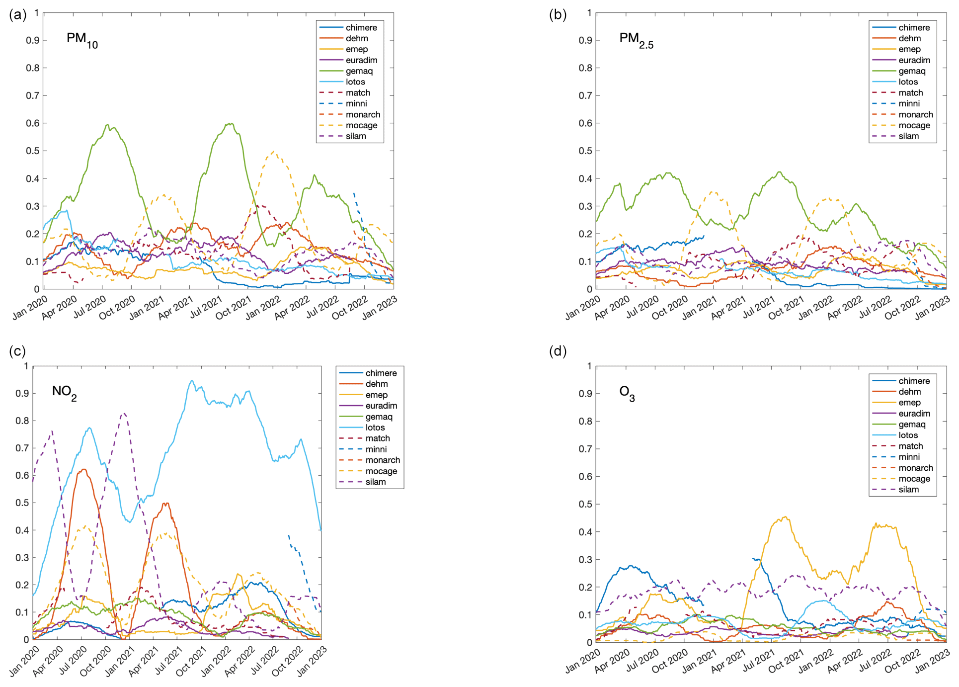
Figure 2 Temporal dependence of model weights for PM₁₀ (a), PM_2.5 (b), NO₂ (c), and O₃ (d). To highlight the temporal dependence, the analysis has been extended over 3 years (from 2020 to 2022, included).

4.3 The added value of the post-processing stages: deterministic-style assessment

4.3.1 Root mean square error, bias, and correlation

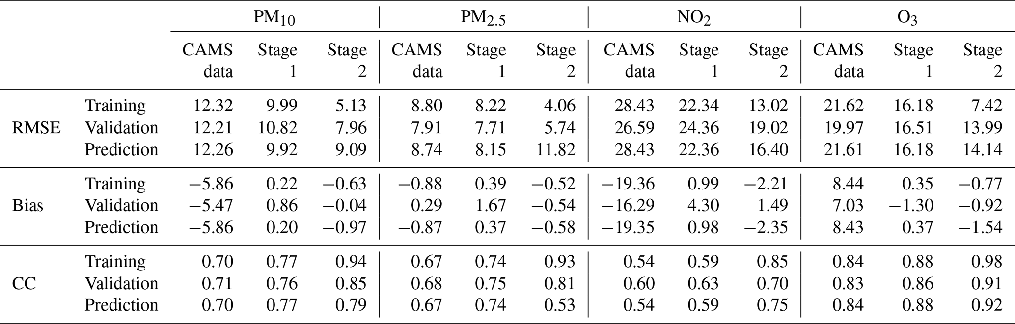
Now we give the results of applying the first and second post-processing stage to the next-day predictions for PM₁₀, PM_2.5, NO₂, and O₃. First, we assessed the performance of the post-processing stages in terms of deterministic scores. Table 2 provides a summary of some of the well-known and widely used scoring measures, that is, root mean square error, bias, and correlation.

The RMSE (root mean square error) and the bias for the training data set for all pollutants were significantly decreased. For example, the RMSE for PM₁₀ was reduced by more than half, but the same was also true for all other pollutants. As can be seen, the raw data of the ensemble for PM₁₀, PM_2.5, and NO₂ are affected by a negative bias, which is almost zero after the application of the first and second post-processing stage. The high values of the correlation coefficients for the training set (above 0.75 for PM₁₀, PM_2.5, and O₃ after the first stage and above 0.85 after the second stage) show that the predicted and observed values are well in agreement. Lower scores are obtained for NO₂, for which only the exploitation of auxiliary spatio-temporal predictors (in the second stage) is capable of raising its value up to 0.85.

However, it is clear that the results obtained for the training data set are not suitable for a fair comparison. A more reliable estimate of the performance of the post-processing stages can be obtained from the validation data set. These data represent 10 % of the measurement stations, randomly selected but stratified according to the type of area in which they are located. The validation data set has not been included in the training process so the results of the validation data set can be considered as a more reliable and truthful estimate of model performance at different spatial locations. In the case of the validation data set, we still have a strong reduction of the RMSE and the almost zeroing of the average bias, as well as a consistently high correlation (usually greater than 0.80), especially after the second stage. The prediction data set refers to the same monitoring stations used for training, but the post-processing framework is used to predict the next-day concentrations. As expected, the performances are lower in this case, even if both the first and second stages generally introduce significant improvements in terms of RMSE, bias, and correlation.

Table 2 Statistics of the cross-validation study. RMSE is the root mean square error; CC is the correlation coefficient. Units of RMSE and bias are expressed in micrograms per cubic metre (µg m⁻³) for all pollutants.

As indicated in Table 1, the measurement stations are unequally distributed with respect to both the type (urban, suburban, or rural) and the geographic location (northern, central, or southern Italy). For example, most measurement stations are located in urban areas, where the concentration of pollutants (especially those of particulate matter and NO₂) is higher. Therefore, an interesting perspective on the analysis of the performance of the statistical post-processing process is to verify whether there is a dependence with respect to the type or geographic location, i.e. whether calibrating these stages with a large number of urban stations leads to a consistent bias adjustment across all monitoring stations (regardless of the type or geographic location) or not. To this end, Fig. 3 shows the bias for all pollutants for the training data set as a function of the type of monitoring station. The results of the CAMS ensemble tend to underestimate the concentration of particulate matter and NO₂, particularly in urban and suburban stations, and overestimate the concentration of ozone (probably related to the underestimation of NO₂ in the same areas), although they tend to be more successful in rural areas. However, the second stage is able to reduce the bias to almost zero in all types of stations without making a distinction between them.

Figure 4 shows the same results but reorganised as a function of geographic location. In this case, the second stage is also able to strongly reduce the bias independently of geographic locations.

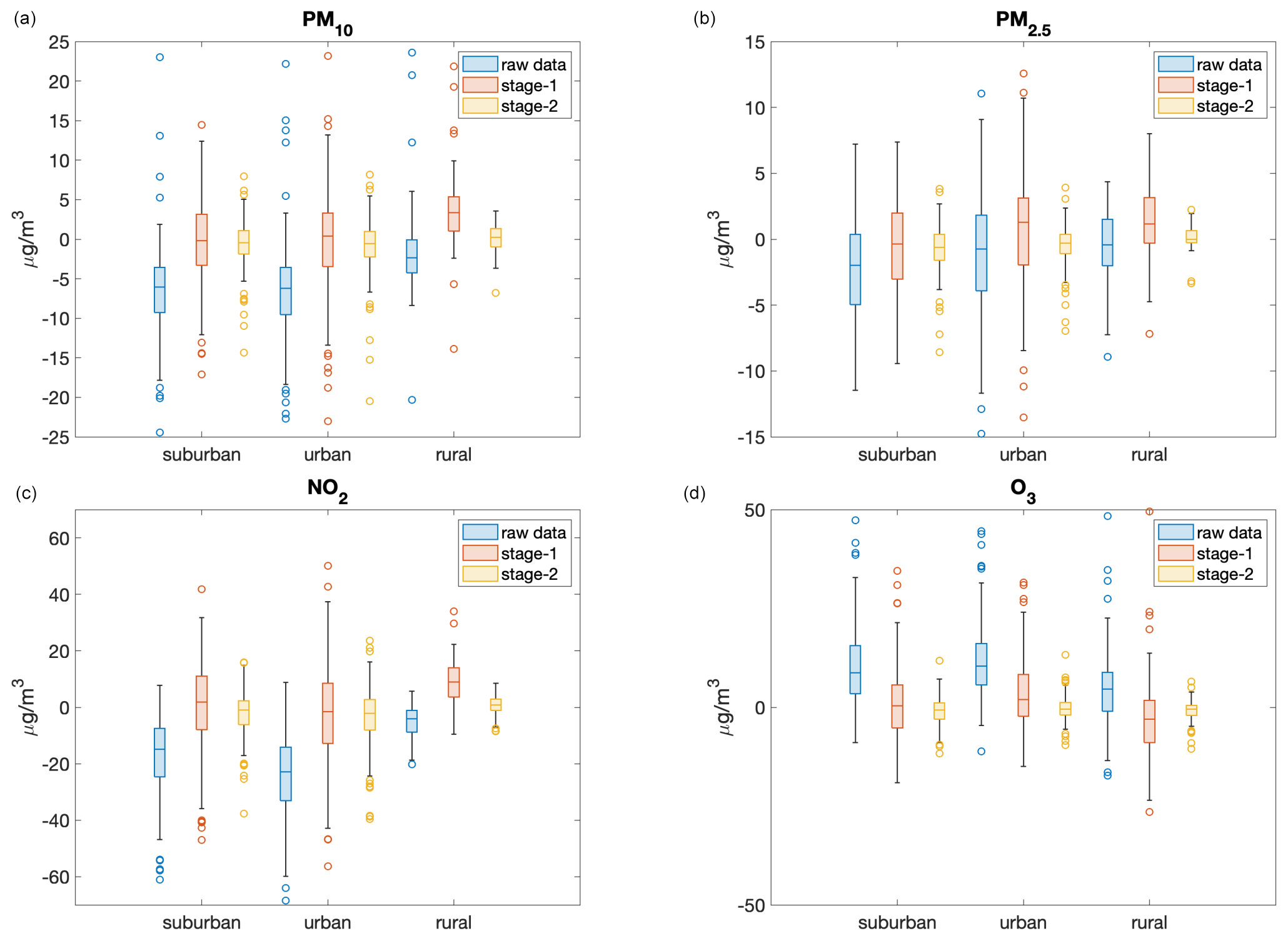
Figure 3 Boxplots for the bias for PM₁₀ (a), PM_2.5 (b), NO₂ (c), and O₃ (d), distinguished according to the type of monitoring station, for the validation data set. The light-blue boxes correspond to the raw results of the CAMS ensemble, whereas the results after the application of the first and second stages are reported as coral and yellow boxes, respectively.

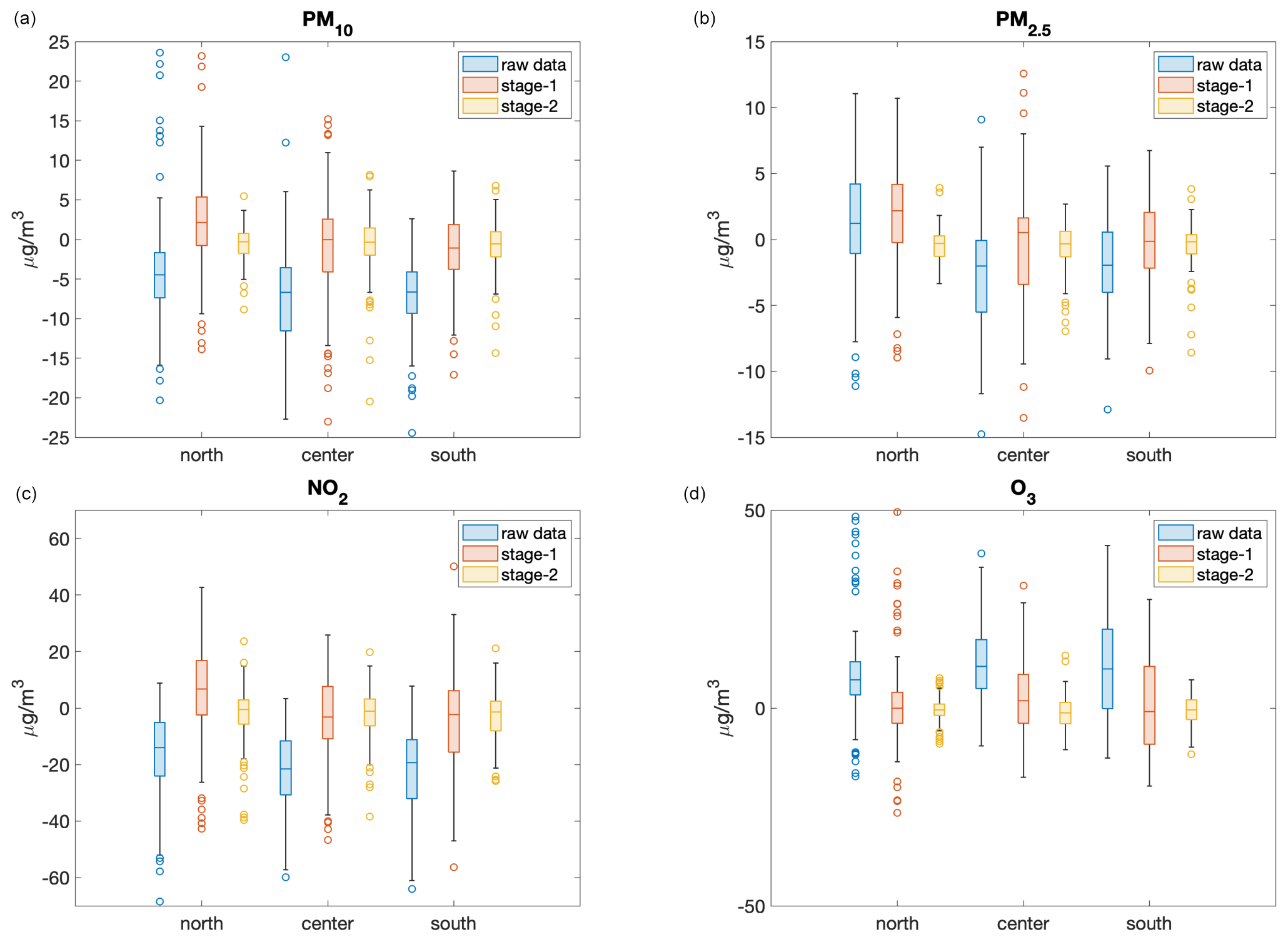
Figure 4 Boxplots for the bias for PM₁₀ (a), PM_2.5 (b), NO₂ (c), and O₃ (d), distinguished according to the geographic location of monitoring station, for the validation data set. The light-blue boxes correspond to the raw results of the CAMS ensemble, whereas the results after the application of the first and second stage are reported as coral and yellow boxes, respectively.

4.3.2 Sensitivity, specificity, and threat score

In order to assess the ability of raw CAMS data or post-processing models to predict the exceedance of a given threshold, we built a confusion matrix, categorising each prediction into a true or false positive or negative outcome. The counts from the confusion matrix were used to define the following indices:

1. sensitivity, also known as true positive rate, defined as the ratio between the number of true positives to the total number of observed exceedances

2. specificity, also known as true negative rate, defined as the ratio between true negatives to the total number of observations not exceeding a given threshold;

3. threat score, also known as critical success index or Jaccard index, defined as the ratio between the number of true positives to the total number of predicted or observed exceedances.

We can consider sensitivity to be a measure of how well our predictions can correctly identify exceedances and specificity as a measure of how well our predictions can correctly identify when observations fall short of a given threshold, while the threat score can be seen as a measure of the overlap between the distribution of observations versus that of predictions. A perfect forecast would take a value of 1 for all of these indices.

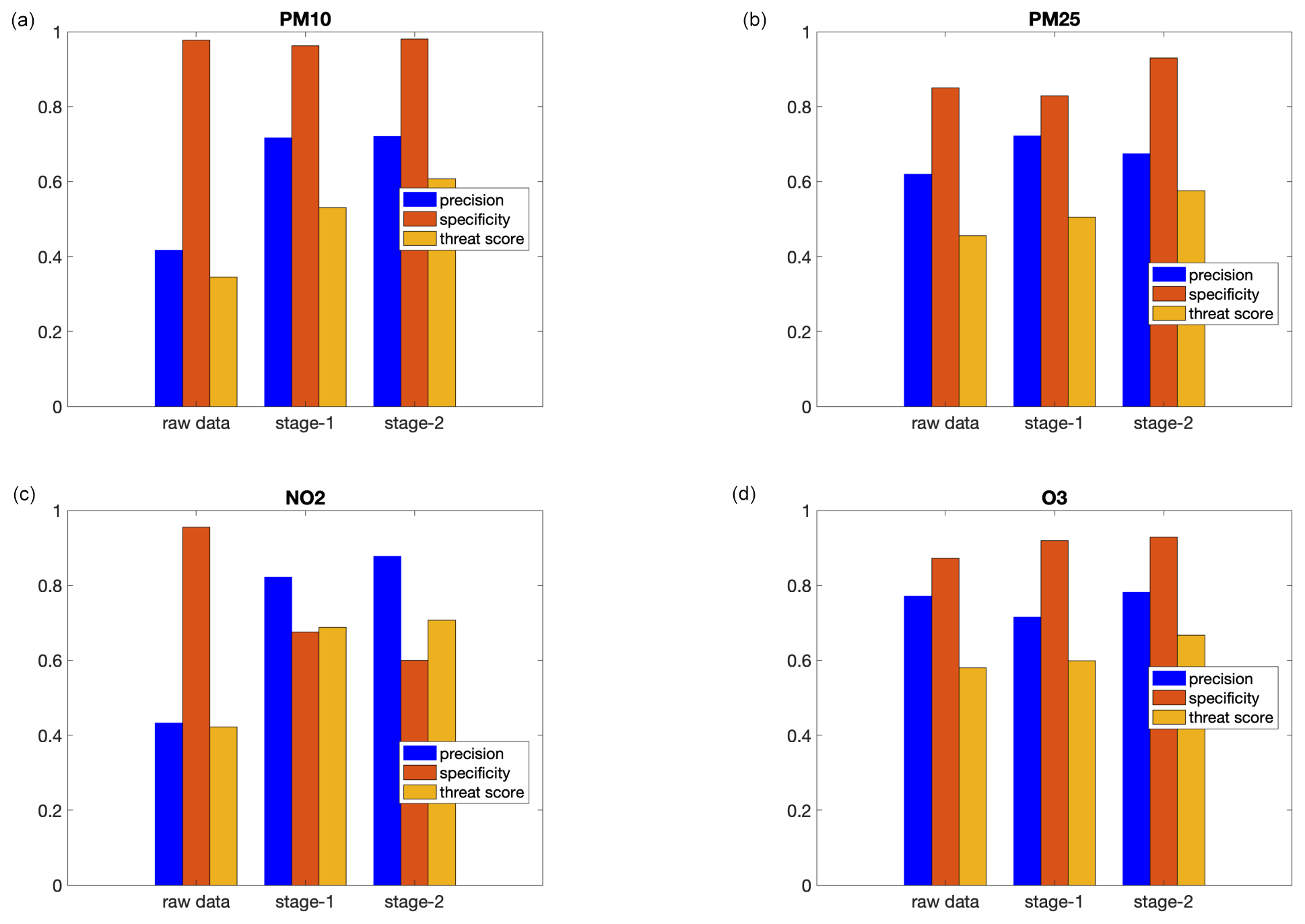
Figure 5 Scores (sensitivity, specificity, and threat score) for the validation data set for PM₁₀ (a), PM_2.5 (b), NO₂ (c), and O₃ (d). The blue bars correspond to the raw CAMS results, while the results after the application of the first and second stage are reported as orange and yellow bars, respectively. The number of exceedances (both for observations and predictions) is defined with respect to the new WHO guidelines: 45 µg m⁻³ for daily PM₁₀, 15 µg m⁻³ for daily PM_2.5, 100 µg m⁻³ for the maximum 8 h daily value for O₃, and 25 µg m⁻³ for daily NO₂ concentration.

The sensitivity, specificity, and threat score indices are plotted in Fig. 5 for the validation data set, where the number of exceedances was defined with respect to the threshold from the new WHO guidelines. The same scores are reported in Fig. S2 of the Supplement.

For PM₁₀ and NO₂, raw CAMS data show a low precision (≈0.4), which is greatly improved after the first and second post-processing stages, achieving a value as high as (or even higher than) 0.8. This means that most events above the threshold are missing from the raw CAMS data but are almost always as expected after post-processing stages.

The increase in sensitivity is not accompanied by a decrease in specificity; in most cases, on the contrary, post-processing increases specificity, that is, the number of events correctly classified as being below the threshold. The only exception is represented by NO₂, for which the specificity decreases after the post-processing stages. However, it should also be said that 25 µg m⁻³ represents a very low threshold for the 1 h daily maximum; therefore, a low specificity in the capture of events at such low concentrations is expected.

4.4 The added value of the post-processing stages: probabilistic-style assessment

RMSE, bias, and correlation look for a match between observations and training, validation, and/or prediction data sets in a stiff mode. However, both the first and the second post-processing stages tailor a statistical dress around results so that we can use probabilities in measuring the properties of our approach.

4.4.1 Reliability and accuracy

First, we checked whether our approach ensures reliability while maintaining high accuracy. In a meteorological context, reliability measures the ability of unbiased predictions to closely follow observed frequencies; that is, for a perfectly reliable forecast, an event declared to occur with frequency p is actually predicted with a proportion p on average (Taylor, 2001). Instead, accuracy refers to the degree to which the prediction is close to the observed data. Both are concerned with the conditional probability of predicting an observation for a given forecast. An in-depth discussion of these and other attributes of probabilistic forecasts can be found in Jolliffe and Stephenson (2011).

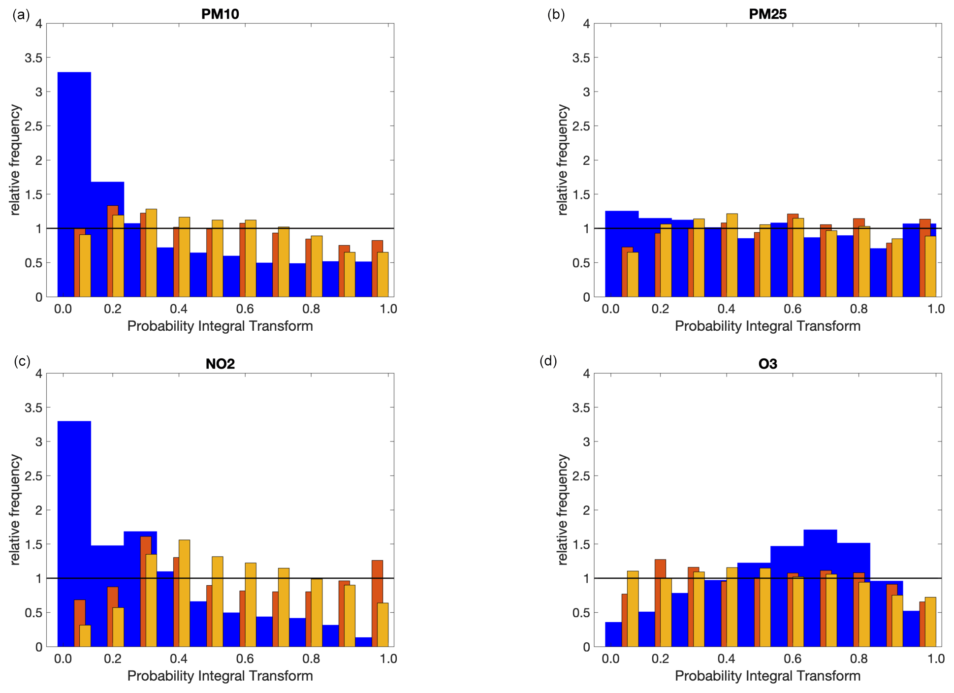
Figure 6 PIT for PM₁₀ (a), PM_2.5 (b), NO₂ (c), and O₃ (d). The blue bars correspond to the raw CAMS results, while the results after the application of the first and second stage to the validation data set are reported as orange and yellow bars, respectively. The orange and yellow bars have been slightly shifted and resized in width so as not to completely overlap the blue bars. The horizontal black lines have been drawn for reference: for a perfectly reliable ensemble, the PIT should be flat, with a relative frequency equal to 1.

Gneiting et al. (2005), in their seminal work, stated that the goal of a well-calibrated probabilistic forecast is to maximise accuracy, subject to reliability. Figure 6 shows the probability integral transform (PIT) for the raw CAMS predictions and after the application of the first and second post-processing stages to the validation data set. Figure S3 shows the same results in the Supplement but for the prediction data set. As can be seen, the PIT histograms for the raw CAMS results for PM₁₀ and NO₂ follow a quasi-monotonic decreasing trend, meaning that the raw CAMS results tend to underestimate observations, while the PIT histogram for O₃ shows an inverted-U-shape profile, meaning overdispersive behaviour, that is, unnecessarily wide prediction intervals that have higher-than-nominal coverage. Conversely, the histograms for the validation and prediction data set, after applying the first and second stages, are closer to a flat profile, showing a more accurate reproduction of the probabilities of occurrence, tending to mitigate both the overall bias and over- or under-dispersion effects.

4.4.2 Credible intervals

The construction of credible intervals from the cumulative distribution function (cdf) is straightforward. For example, the 25th and 75th percentiles of cdf form the lower and upper endpoints of the 50 % central prediction interval, respectively, from which the sharpness, that is, the spread around the predicted value, can be evaluated. For a well-calibrated ensemble, the higher the accuracy is, the more data are concentrated around the predicted value, and the more value the model adds.

We estimate the 25th and 75th percentiles from the posterior distributions of the first and second stages for each pollutant and compare these results with the interval from the 25th to the 75th percentile from the raw CAMS ensemble data. Table 3 shows the average widths of the 50 % probability interval for the raw CAMS data and after the application of the first and second post-processing stages. As can be observed in this table, after the application of the first stage, the credibility interval tends to widen – i.e. the calibrated data show a much smaller bias (see Table 2) – but at the cost of widening the credibility interval, making the prediction less accurate. On the other hand, the effect of applying the second stage through the exploitation of spatial and spatio-temporal predictors is not only to improve the accuracy of the forecast but also to make the forecast sharper, narrowing the credibility interval. This range is also generally smaller than that obtained from the raw CAMS data. For example, the credibility interval for all pollutants is roughly halved for the validation data set, going from 8.3 to 4.4 µg m⁻³ for PM₁₀, from 8.3 to 4.4 µg m⁻³ for PM₁₀, from 5.3 to 3.3 µg m⁻³ for PM_2.5, from 17.9 to 10.8 µg m⁻³ for NO₂, and from 13.5 to 15.1 µg m⁻³ for O₃.

4.5 Example of applications

Finally, we want to conclude this section with two examples of potential applications of our post-processing analysis, i.e. (a) interpolation at high spatial resolution and (b) detection of non-compliant areas.

Interpolating data that have been processed in locations not directly observed must be done with consideration of the issues that come with space–time inhomogeneities and seasonal dependencies. For example, PM₁₀ and PM_2.5 are known to be higher during the winter period, especially for urban stations. On the contrary, concentrations in remote stations are relatively low, with a seasonal cycle that favours higher concentrations during the summer season. This is a well-known phenomenon, linked to the activation of convective processes that transport particles emitted at low levels to higher altitudes during the summer period; conversely, urban areas are affected by higher concentrations of particulate matter during the winter period due to condensation phenomena at low temperatures and atmospheric subsidence (Marinoni et al., 2008). It is also known that NO₂ is a short-lived gas in the atmosphere, with a lifetime of several hours, especially in the boundary layer during the daytime (Beirle et al., 2011; Lu et al., 2015). Since NO_x emission sources are generally clustered near densely populated urban areas, strong spatial gradients in geographical distribution can be observed from space (Crippa et al., 2018). The relatively low spatial resolution of the CAMS data cannot resolve these steep spatial gradients, and simply merging the results (using equal or unequal weights) into a median prediction cannot remedy this issue.

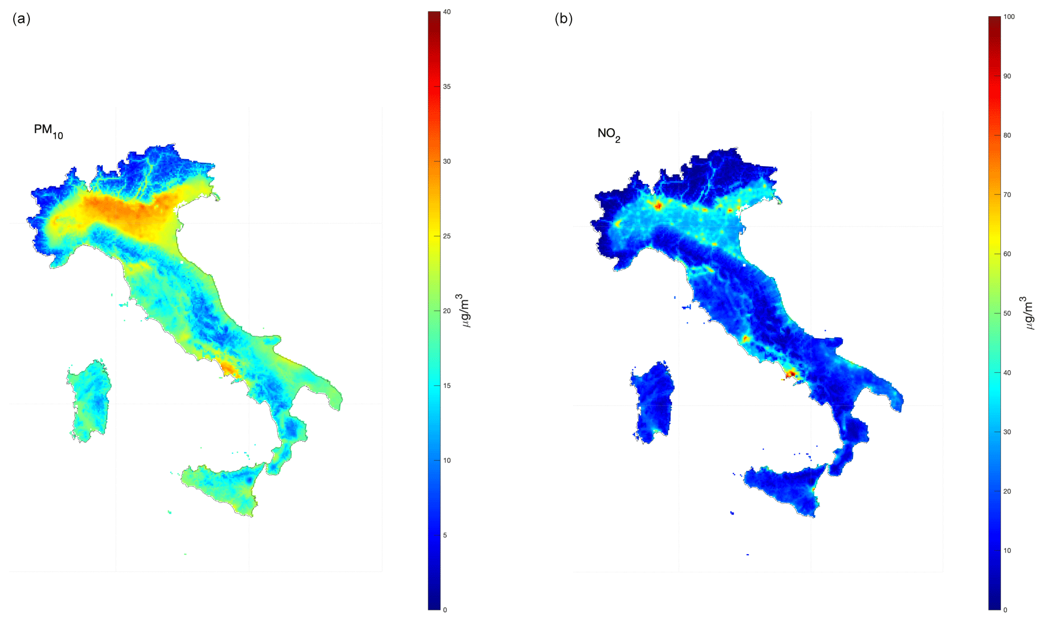
Figure 7 Median PM₁₀ concentration map (a) of daily means and median NO₂ concentration map (b) of 1 h daily maximum in 2022 after the application of the second post-processing stage and estimated over a regular 4 × 4 km grid resolution.

As shown in Sect. 4.3 and 4.4, the forecasts of the raw CAMS data set show significant biases for all pollutants; for example, the raw CAMS data, even when the mean of the ensemble is considered, cannot follow the seasonal cycle for PM₁₀, especially for urban stations where the peaks can be higher than 60 µg m⁻³. In contrast, statistical post-treatment is capable of rapidly adapting the forecast to the synoptic evolution and removing bias, independently of the type and density of monitoring stations. These properties are also retained when analysing data for the validation data set, that is, for those stations not directly involved in the training phase. It is reasonable to expect similar performance in unmonitored areas as in, for example, areas corresponding to a regular grid. With regard to this aim, the calibrated ensemble average from stage 1 was interpolated onto a 4 × 4 km regular grid (using a bi-linear interpolation), and the post-processing from stage 2 was applied using the spatio-temporal predictors estimated at the cell centres of this grid. Figure 7 shows the concentration maps of two exemplary pollutants, PM₁₀ and NO₂, estimated on the 4 × 4 km regular grid for the Italian peninsula.

It is interesting to compare these figures with the median forecast from raw CAMS data. Figure S4 in the Supplement show the same results but from the raw CAMS data set. In Fig. S4. the pattern is that expected, but it is also clear that the resolution of the CAMS ensemble does not allow one to capture the details on a finer scale, and it obviously does not make much sense to interpolate these data at higher resolutions. Unlike raw CAMS data, the second stage of the statistical post-processing treatment inoculates new information, which allows one to capture finer details, making the space–time interpolation process more realistic and precise (at least for the monitored stations included in the validation process). This applies to both PM₁₀ and NO₂, where the effects of urban areas and the road network are more evident. Figure S5 show the median values for PM_2.5 and O₃ after post-processing treatment.

A second application concerns the possibility of accurately highlighting the non-compliant areas with a spatial resolution higher than that made available by the CAMS models. The WHO recently revised the recommended guidelines to protect the health of the population (WHO, 2021), and in October 2022, the European Commission committed to further improving air quality and aligning air quality standards with WHO recommendations (EC, 2022). According to the proposal of the European Commission (EC), partial alignment (the so-called policy option I-3) was chosen because it corresponds to the highest cost–benefit ratio, and the EC recommends the entry into force of this new policy option by 2030, balancing the need for rapid improvements with the need to ensure sufficient response times and coordination with key related policies that will deliver results in 2030 (such as the Fit for 55 package of climate change mitigation policies).

Specifically, in the EC proposal, the new limit values for the protection of human health to be achieved by 2030 are 45 µg m⁻³ for the PM₁₀ daily limit, not to be exceeded more than 18 times per calendar year, and 25 µg m⁻³ for the PM_2.5 daily limit, not to be exceeded more than 18 times per calendar year. The post-processing method proposed in this work is ideal for highlighting non-compliant areas, for example by using the corrected daily averages for 2022 to detect which areas need to be subject to increased containment measures to meet the 2030 limits.

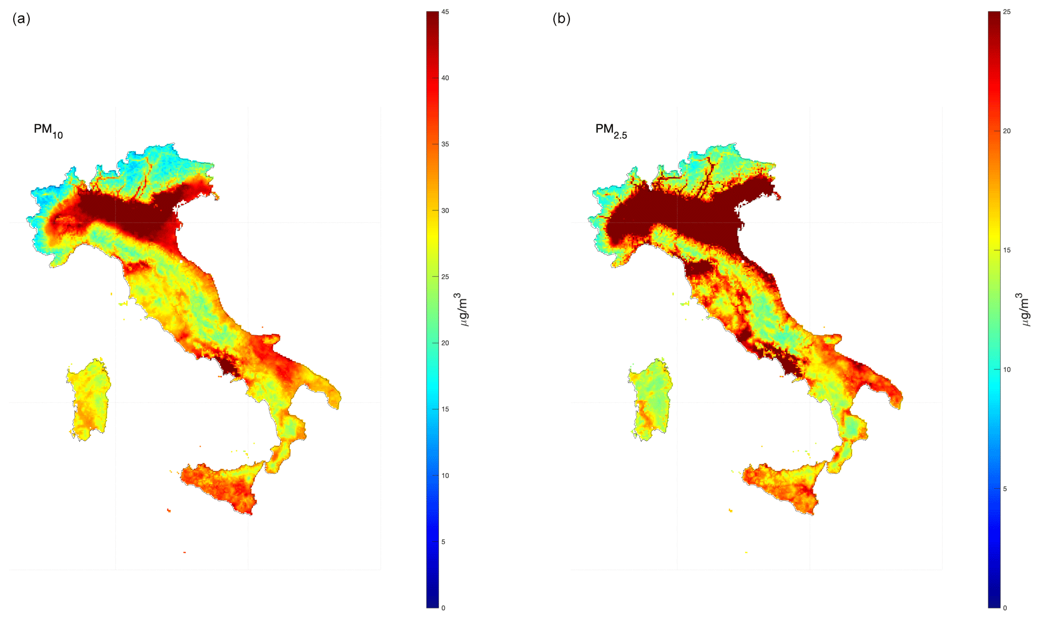
Figure 8 The 95.1st percentile of PM₁₀ (a) and PM_2.5 (b) after the application of the second post-processing stage and estimated over a regular 4 × 4 km grid resolution.

Table 3 Average width for the 50 % probability interval around the predicted value for the estimation data set (first row) and validation data set (second row) and in prediction mode (third row). Units are expressed in micrograms per cubic metre (µg m⁻³) for all pollutants.

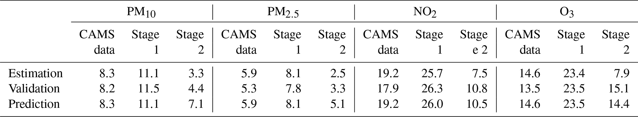
Figure 8 shows the map of the 95.1st percentile of daily means for PM₁₀ and PM_2.5. The deep-red colour marks the areas for which the daily PM₁₀ concentration exceeds the threshold of 45 µg m⁻³ more than 18 times in 2022 (and the threshold of 25 µg m⁻³ for PM_2.5). Not surprisingly, large areas with concentrations above the 2030 threshold for PM₁₀ are observed in the Po Valley and other urban areas (especially the urban area of Naples). Similarly, the PM_2.5 threshold is particularly challenging to respect. The entire Po Valley and the main urban areas (the metropolitan areas of Florence and Naples) all exceed the PM_2.5 threshold so strict containment measures will be necessary for a large part of the Italian peninsula.

According to the results of this work, more than 21 % of the Italian peninsula exceeds the 2030 threshold for PM_2.5.

Figure S6 show the 95.1st percentile of the highest 8 h daily maximum for O₃ after post-processing treatment. The new EC proposal established a threshold of 120 µg m⁻³ for this pollutant, but more than 37.3 % of the Italian peninsula does not comply with this limit. In this case, not only the Po Valley and the main urban areas are affected by this problem; several rural areas and those corresponding to the highest altitudes are also affected.

5 Conclusions

In this work, the effectiveness of statistical post-processing techniques aimed at improving the accuracy and reliability of the predictions of the air quality models of the CAMS suite have been tested. It is well known that the CAMS suite (currently made up of 11 members), while representing the state-of-the-art of atmospheric modelling, shows significant biases; hence, it is advisable to adopt post-processing techniques that are statistically reliable and computationally inexpensive to cope with operational constraints. Furthermore, predictions are currently available with moderate spatial resolution (0.1^∘ × 0.1^∘) and may miss steep spatial gradients that occur in the vicinity of large urban areas and industrial sites.

In order to ameliorate these problems, a statistical post-processing technique was developed and applied to the Italian region, capable of correcting both the bias and the reliability of ensemble predictions. Concentrations of the main air pollutants, PM₁₀, PM_2.5, NO₂, and O₃, were taken into account, and a new two-stage post-processing approach was designed, able to meet operational constraints. In the first stage, the ensemble data were combined together through minimisation of the continuous ranked probability score (crps) on the training data. During the second stage, the ensemble prediction was corrected by exploiting additional spatio-temporal predictors within a framework based on the INLA-SPDE approach. The post-processing stages make use of a short training period (3 d) so as to rapidly adapt to changes in meteorological or emission conditions and to apply simultaneously to all monitoring stations.

The post-processing approach is computationally inexpensive. For example, the application of the post-processing method for 1 d usually takes less than 40 s on a typical desktop computer (we used an iMac computer equipped with a 3.4 GHz Intel i5 quad-core processor and 16 GB 2.4 GHz DDR4 memory). This computational time is competitive with respect to other approaches (for example, complex spatio-temporal hierarchical models within a Markov chain Monte Carlo framework), mainly due to the efficient use of sparse matrices and the Laplace approximation for numerical integration schemes (Bakka et al., 2018).

The validation procedure shows that the post-processing stages were able to remove systematic biases, improve accuracy, and provide reliable forecasts. Moreover, the global approach allowed the application of the INLA-SPDE framework to a regularly spaced grid (with a resolution higher than that of the original CAMS members), highlighting the regions in which exceedances occur.

The post-processing correction process has been applied to the measurement stations for the year 2022 for Italy, but this procedure can be easily generalised to any spatial and temporal region. Because of its flexibility, we also expect that this approach is prone to adapt in real time to fast changes in meteorological conditions and/or abrupt changes in pollutant emissions.