Warming effects of reduced sulfur emissions from shipping

The regulation introduced in 2020 that limits the sulfur content in shipping fuel has reduced sulfur emissions over global open oceans by about 80 %. This is expected to have reduced aerosols that both reflect solar radiation directly and affect cloud properties, with the latter also changing the solar radiation balance. Here we investigate the impacts of this regulation on aerosols and climate in the HadGEM3-GC3.1-LL climate model. The global aerosol effective radiative forcing caused by reduced shipping emissions is estimated to be 0.13 W m⁻², which is equivalent to an additional ∼50 % to the net positive forcing resulting from the reduction in all anthropogenic aerosols from the late-20th century to the pre-2020 era. Ensembles of global coupled simulations from 2020–2049 predict a global mean warming of 0.04 K averaged over this period. Our simulations are not clear on whether the global impact is yet to emerge or has already emerged because the present-day impact is masked by variability. Nevertheless, the impact of shipping emission reductions either will have already committed us to warming above the 1.5 K Paris target or will represent an important contribution that may help explain part of the rapid jump in global temperatures over the last 12 months. Consistent with previous aerosol perturbation simulations, the warming is greatest in the Arctic, reaching a mean of 0.15 K Arctic-wide and 0.3 K in the Atlantic sector of the Arctic (which represents a greater than 10 % increase in the total anthropogenic warming since pre-industrial times).

1 Introduction

Globally ships emit around 10–13 Tg yr⁻¹ of sulfur dioxide (SO₂) into the atmosphere in recent years, which accounts for about 14 % of global SO₂ emissions from all sectors in both ECLIPSE (Klimont et al., 2017) and CEDS (Hoesly et al., 2018) datasets. In the atmosphere, SO₂ is oxidised to form sulfate, which either condenses on the existing aerosol particles or forms new particles, and hence contributes additional aerosol mass and number. These particles directly modify the Earth's energy budget by scattering solar and terrestrial radiation and indirectly affect it through changing the cloud microphysical (droplet numbers and sizes affecting the reflectivity) and macrophysical (cloud cover, height, liquid and ice water paths) properties. Over the ocean, due to the dark surface (low albedo), any change in aerosol and cloud reflectivity can potentially have a large impact on the Earth's energy budget.

Ship exhausts are known to form ship tracks, which are the linear features of enhanced cloudiness or cloud brightness up to hundreds of kilometres in length that are sometimes clearly visible in satellite images, typically in the regions of marine stratocumulus clouds (e.g. Conover, 1966; Coakley et al., 1987; Toll et al., 2019; Diamond et al., 2020). Although the majority of ocean-going ships do not leave identifiable ship tracks, the sulfur species will still be widely dispersed and potentially cause significant, but less apparent, aerosol–cloud interactions that modulate the Earth's energy budget (Possner et al., 2018; Manshausen et al., 2022).

Particulate matter originating from shipping emissions causes substantial air pollution in coastal areas of the world, causing an estimated 400 000 premature deaths every year (Sofiev et al., 2018). To mitigate this, the United Nation's International Maritime Organisation (IMO) set sulfur emission control areas (SECAs) in inland seas in northern Europe and along the coasts of North America in which sulfur emissions from shipping were limited by specifying a maximum fuel sulfur content of 0.1 % by mass. In addition, from January 2020, the IMO further restricted the maximum fuel sulfur content of ships in all ocean regions outside the SECAs to 0.5 % of fuel mass. It is claimed that this will prevent about 600 000 premature deaths in the coming years (Corbett et al., 2016). This is a large step change from the previous regulation that allowed fuel sulfur contents of up to 3.5 % which will substantially affect shipping sulfur emissions and potentially atmospheric composition and climate.

To investigate the effects of the new emission regulation on atmospheric composition and the responses of the climate, we performed two ensembles of coupled climate model simulations with and without the sudden emission reduction due to the IMO regulation change after 2020.

2 Methods

2.1 Model

We use the HadGEM3-GC3.1-LL (also called HadGEM3 N96ORCA1; Kuhlbrodt et al., 2018), the low-resolution version of the HadGEM3 version 3.1 global coupled model (Williams et al., 2017), where the atmosphere model with 1.875°×1.25° horizontal resolution and 85 vertical levels is coupled with the 1° resolution NEMO ocean model (Madec et al., 2017). The atmosphere model involves the UKCA scheme (O'Connor et al., 2014), which includes the GLOMAP-mode two-moment aerosol model (Mann et al., 2010). Black carbon (BC), organic carbon (OC), sea salt (SS), and sulfate (SU) aerosols are simulated in GLOMAP-mode where microphysical interactions between different aerosol species and sizes are represented. Mineral dust is included separately in the CLASSIC bin scheme (Bellouin et al., 2007; Woodward, 2001).

SO₂ is oxidised to form sulfuric acid via the gas-phase reaction with OH radicals in the troposphere or through the aqueous-phase reactions with O₃ and H₂O₂ in cloud droplets. Gas-phase sulfuric acid then either condenses on the existing aerosol particles or forms new particles through binary homogeneous nucleation throughout the atmosphere (Vehkamäki et al., 2002) or through organically mediated nucleation in the boundary layer (Metzger et al., 2010). In this model, oxidant concentrations are prescribed and do not change by these reactions. A total of 2.5 % of the SO₂ from both anthropogenic and natural sources is assumed to be emitted as primary aerosol particles to represent subgrid-scale oxidation and condensation.

2.2 Experimental design

We set up two 35-year ensembles of simulations between 2015 and 2049 that differ in the change in shipping SO₂ emissions after 2020. Concentrations of well-mixed greenhouse gases and reactive gases including oxidants were prescribed following the ScenarioMIP SSP1-2.6 scenario (O'Neill et al., 2016).

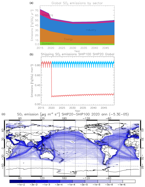
Figure 1 SO₂ emissions used in the simulations. (a) Global annual SO₂ emissions by sector in the SHIP20 scenario from 2015 to 2050 based on the ECLIPSE v6b dataset. (b) Global monthly shipping SO₂ emission pathways in the SHIP100 (blue) and SHIP20 (red) scenarios for the same period. (c) Change in SO₂ emissions in 2020 (SHIP20 minus SHIP100 emissions). Global aerosol emissions from transport, waste, and flaring are included in the dataset but can hardly be seen in (a) due to their relatively minor contributions, although they can be regionally important.

Our base case scenario generally follows the ECLIPSE v6b scenario (Klimont et al., 2017) but with a small modification. In ECLIPSE v6b the global shipping SO₂ emissions fall from 10.1 Tg SO₂ (14 % of anthropogenic emissions) in 2015 to 2.1 Tg (4 %) in 2020, consistent with the sulfur emission reduction by the IMO 2020 regulation. However, in our simulations, we repeated the 2015 emissions for 2016–2019, instead of smoothly interpolating the ECLIPSE v6b values between 2015 and 2020, to represent the sudden reduction due to the regulation change in the year 2020. We call this scenario SHIP20 because it includes the reduction in shipping SO₂ emissions to 20 % of its pre-2020 value. In the other (counterfactual) scenario, we repeated the shipping SO₂ emissions of 2015 until the end of the simulation. We call this SHIP100. Figure 1 shows the emission pathways in both of these scenarios as well as the difference between them in space and time.

We used the ECLIPSE v6b scenario for emissions of primary carbonaceous aerosols (black carbon and organic carbon) from anthropogenic and biofuel sources. Emissions of primary carbonaceous aerosols from biomass burning, volcanic emissions of SO₂, and biogenic monoterpenes (a precursor gas of secondary organic aerosol) were also prescribed according to the SSP1-2.6 scenario. Emissions of marine dimethyl sulfide (DMS), a precursor of sulfate aerosol, are calculated interactively within the model (Mulcahy et al., 2020) as a function of surface wind speeds and prescribed surface seawater DMS concentrations given by Lana et al. (2011). Sea salt emissions are calculated interactively within the model using wind speeds over the sea.

The emission reductions in various aerosols and precursor gases due to the COVID-19 pandemic were not included and are not expected to be significant on the decadal timescales of interest here.

A total of 12 pairs of simulations were created under the two emission scenarios, each starting from slightly different initial conditions taken from the HadGEM3-GC3.1-LL Coupled Model Intercomparison Project (CMIP6; Eyring et al., 2016) historic simulations. By creating paired simulations in two ensembles we aim to preclude sampling bias caused by the choice of initial conditions. The use of ensembles of 35-year simulations allows us to examine the transient response of the climate system.

Figure 2 Change in ensemble-mean sulfate aerosol column burden [mg m⁻²] from SHIP100 to SHIP20. The differences are statistically significant at a 95 % confidence level in paired t tests everywhere except the hatched regions.

Figure 3 Effective radiative forcing (W m⁻²) from shipping sulfur reduction (SHIP20−SHIP100), calculated from atmosphere-only nudged simulations. The plot has been smoothed by averaging each grid box value with the values from its neighbouring grid boxes.

2.3 Estimation of temperature changes from pre-industrial baseline

Global and regional mean temperature changes between the pre-industrial (PI) and present-day (PD) time periods were estimated using the PI temperatures of the four-member CMIP6 HadGEM3-GC3.1-LL ensemble (Gillet et al., 2021) as a baseline, which were calculated as the ensemble mean of the CMIP6 historical simulations for the period of 1850–1900. This ensemble gives an historic global warming of about 1.1 K from 1850–1900 to 2010–2019, which is close to the centre of the multi-model range of 0.9–1.3 K and the observed range of 1.0–1.3 K (Gillet et al., 2021). The 12 members of each of our two ensembles (one for SHIP20 and one for SHIP100) were generated using different start dumps from the four-member CMIP6 HadGEM3-GC3.1-LL ensemble of Gillet et al. (2021) as initial conditions; four members used dumps from 1 January 2013, four from 1 January 2014, and four from 1 January 2015. Hence the PI temperatures of the Gillet et al. (2021) ensemble are an appropriate baseline since our simulations represent a continuation of those runs using the same model.

2.4 Estimation of effective radiative forcing

Aerosol effective radiative forcing (ERF) was estimated from global atmosphere-only UKESM1 (United Kingdom Earth System Modelling) simulations nudged to ERA-Interim analysis data (Berrisford et al., 2011). Two simulations were conducted for the period of 9 years from 2015 to 2023, with shipping emissions held constant at 2015 and 2020 levels, corresponding to SHIP100 and SHIP20 scenarios, respectively. The simulation data from the last 8 years were utilised, with the data from 2015 excluded. The ERF was calculated following the methodology outlined in Ghan (2013) and by comparing the results obtained from the two simulations.

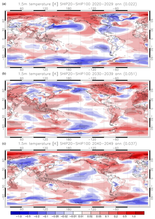
Figure 4 Differences in time-averaged ensemble annual mean 1.5 m temperatures between the SHIP20 and SHIP100 simulations in the 2020s (a), 2030s (b), and 2040s (c). The hatching shows where the differences between the two ensembles are statistically significant at a 95 % confidence level in paired t tests. DJF and JJA seasonal averages are shown in Figs. S1 and S2 in the Supplement.

3 Results

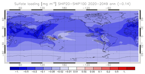
Figure 2 shows the difference in ensemble-mean sulfate aerosol column burden (vertically integrated mass per unit area) between the SHIP100 and SHIP20 scenarios averaged over the entire simulation period. The global mean reduction is 0.14 mg m⁻², corresponding to 4.6 % of the case in SHIP100. The spatial pattern of changes in sulfate burden largely follows the pattern of emissions (Fig. 1c) but with greater spreading due to transport of SO₂ and the resulting aerosol. The strongest reductions can be seen in the large coastal region of Southeast Asia followed by in the Mediterranean and around the Arabian Peninsula. Relatively large reductions are seen over the large region covering the eastern tropical Atlantic, Europe and north Africa, the tropical Indian Ocean, and the West Pacific.

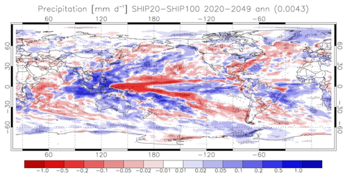
Figure 5 Differences in ensemble-mean annual precipitation between SHIP20 and SHIP100 simulations averaged for 2020–2049.

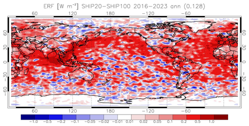
Figure 3 shows the aerosol ERF (SHIP20−SHIP100) caused by the reduction in sulfur emissions quantified from the two parallel global atmosphere-only nudged simulations for 2016–2023. The global annual mean aerosol ERF is 0.128 W m⁻², with an interannual standard deviation of 0.016. Strong positive ERF can be seen extending from northern Indian Ocean through Southeast Asia to China, along the North Pacific shipping corridor from Japan, and around the Iberian Peninsula and Morocco, consistent with the reduced sulfur emission in Fig. 1c and sulfate burden in Fig. 2.

Although the emission reductions equate to only about 14 % of global SO₂ emissions from all sectors, this forcing is about 50 % of that caused by reductions in all anthropogenic aerosol emissions since the 1990s when the magnitude of the negative global aerosol forcing peaked. This is based on the weighted historical time series of CMIP6 forcings in Smith et al. (2021), which estimates a 1990–2020 aerosol ERF of 0.25 W m⁻².

Figure 4 shows the global map of the difference in annual mean 1.5 m temperatures between the two scenarios (SHIP20−SHIP100) averaged over three 10-year periods: 2020–2029, 2030–2039, and 2040–2049. Figures S1 and S2 show the same but for December–February (DJF) and June–August (JJA). These plots show statistically significant warming in the 2030s and 2040s in the tropical eastern Indian Ocean to western Pacific Ocean region, around the Mediterranean, in eastern North America, and in the Atlantic Ocean north of 60° N. Although these locations are not necessarily consistent in these two decades, many of these regions correspond to the regions with relatively strong positive ERFs (Fig. 3).

An interesting feature of the distribution of temperature changes is a warming in the tropical eastern Indian Ocean to western Pacific Ocean and a cooling in the central to eastern Pacific. Surface temperatures show very similar features (not shown). This warming and cooling pattern corresponds to the pattern of increased and decreased rainfall in the tropics between 90° E and 135° W (Fig. 5). These resemble the anomalous patterns seen during La Niña. Figures S3 and S4 show that this pattern corresponds to changes in top-of-atmosphere longwave flux and high-cloud amount in the simulations. It is a unique feature that the longwave response dominates the shortwave in this region, while it is opposite globally and in most other regions, and we attribute this to the change in the high-cloud amount. Furthermore, Fig. S5 indicates that these changes are associated with the strengthening of Walker circulation, with enhancements of convergence of low to mid-level horizontal wind around 125° E (top panel), upward motion over the western Pacific (100–125° E) and downward motion over the central Pacific (130° E–160° W; bottom panel) in the SHIP20 ensemble. The increase in high-cloud amount is hypothesised to be due to the increased upward moisture transport over the western Pacific (Fig. S5) caused by the enhanced upward motion and increased convection. A unique feature of increased aerosol column burden is seen over New Guinea in Fig. 2, which is likely due to reduced rainfall there. Together with the ocean processes such as changes in surface currents and the zonal sea surface temperature (SST) gradient in the equatorial Pacific (not shown), the mechanism causing conditions like La Niña is consistent with the positive Bjerknes feedback (Bjerknes, 1969; Rädel et al., 2016) that explains how the El Niño–Southern Oscillation (ENSO) anomaly is reinforced.

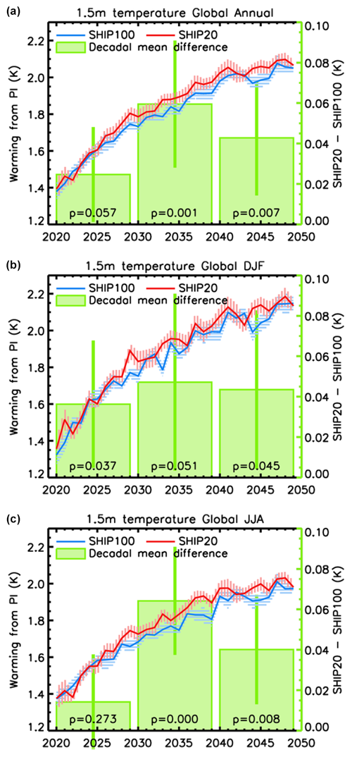
Figure 6 The evolution of global-averaged ensemble-mean 1.5 m air temperatures in the SHIP20 (red line) and SHIP100 (blue line) simulations compared to the 1850–1900 means. The shading around the lines shows the 1 standard error range. The green rectangles show the differences in the decadal means (secondary y axis) and their 1 standard error range (vertical green lines) for annual (a), DJF (b), and JJA (c) data. P values in paired t tests for the decadal means are shown near the bottom of the corresponding green rectangles.

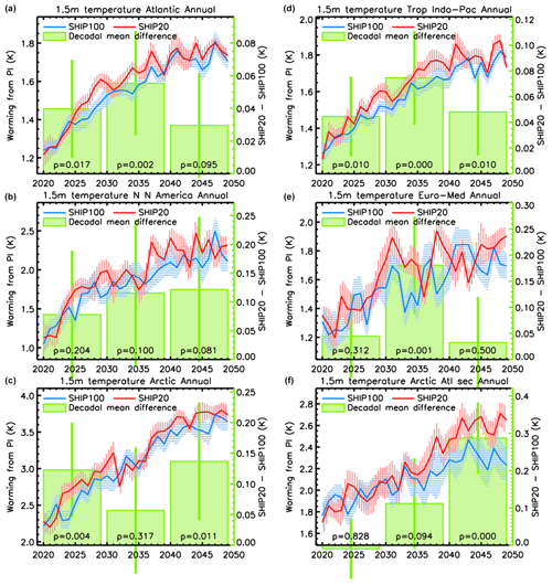
Figure 7 Same as Fig. 6 but for regional annual averages. From top left to bottom right: Atlantic (50° S–0, 45° W–15° E; 0–50° N, 70–10° W), tropical Indian and Pacific oceans (15° S–20° N, 45–150° E), northern North America (40–70° N, 135–60° W), Europe and Mediterranean (30–70° N, 10° W–30° E), Arctic (60–90° N, 180° W–180° E), and Atlantic sector of the Arctic (60–80° N, 90° W–30° E). DJF and JJA averages are shown in Figs. S6 and S7.

Figure 6 shows the global time evolution of the ensemble-mean warming in the two scenarios compared to the pre-industrial baseline, decadal mean differences between the two scenarios, and measures of statistical significance (standard errors and p values in paired t tests). According to this, the global annual mean warming exceeds 1.5 K around 2023 regardless of the shipping emissions change. The reduction in shipping sulfur emissions (SHIP20 compared to SHIP100) causes additional warming starting in the late 2020s. In the following decades the additional warming by the shipping emissions reduction is 0.04–0.05 K and is statistically significant (p=0.001 in 2030s and 0.007 in 2040s). It also suggests that the shipping emissions reduction could be an important factor that determines whether global warming reaches 2.0 K in the 2040s. Seasonally, the warming is somewhat larger and more significant in northern summer (0.04–0.06 K; p=0.00–0.01) than in winter (∼0.04 K; p∼0.05). This is likely due to the large reduction in aerosol loading in the Northern Hemisphere having stronger effects in northern summer, when the solar radiation is more intense.

Figure 7 shows the regional time evolutions of the ensemble-mean warmings for the Atlantic, tropical Indian and Pacific oceans, northern North America, Europe, the Arctic, and the Atlantic sector of the Arctic. Figures S6 and S7 show the same things but for DJF and JJA. Statistically significant additional warming due to shipping sulfur reduction can be seen in several regions and decades, although the inconsistency is seen between the 2030s and 2040s likely due to the relatively small ensemble size and the small forcing compared to the internal variability. The additional warming can be over 0.1 K over the northern North America, Europe and the Mediterranean, and Arctic regions (Fig. 7c, d, and e) and up to 0.3 K in Atlantic sector of the Arctic (Fig. 7f).

4 Discussion and conclusions

Our results suggest that how we experience global warming in the next few decades will be dependent on both the climate impact of SO₂ shipping cuts and natural variability (Figs. 6 and 7) as well as the underlying greenhouse-gas-driven climate change. At the regional scale (Fig. 7) the magnitude of the climate impact appears to emerge and sometimes reduce again through time. This suggests that we would need a larger ensemble size to more fully isolate the climate change signal (or potentially interesting dynamical feedbacks which have yet to be identified). The simulations show that the climate impact of SO₂ cuts takes a few years to emerge, which is consistent with the climate response to other step changes in forcings in other contexts. For example, Fig. 1b in Andrews et al. (2019) shows the global temperature response to a step change in CO₂ (instantaneous quadrupling in this case) for a wide range of CMIP models (including the UKESM1 model used in this study). This shows that UKESM realises 44 %, 59 %, and 68 % the longer-term climate response within 5, 10, and 20 years of a step change in forcing, respectively. However, given the effect of sub-decadal variability on the signal in other parts of the record, caution is needed as this may alternatively reflect variability masking the initial response. As such, it is unclear whether we would expect the real world to already be experiencing the warming impact of SO₂ shipping cuts or whether the signal will emerge in the next few years, which has implications for interpreting their impact.

If the global climate impact of SO₂ shipping cuts will emerge in the next few years, as our Fig. 6 results suggest, then this has consequences for our ability to achieve our global warming targets. Whilst the global temperature impact is modest in the context of longer-term global warming, ranging from 0.04 to 0.05 K (Fig. 6), it becomes more relevant when we consider global targets of 1.5 or 2 K. The year 2023 is estimated to have been around 1.45 K warmer than average conditions of 1850–1900 (World Meteorological Organization, 2024). Annual temperatures are subject to year-to-year variability, with El Niño conditions contributing to 2023 temperatures; hence long-term warming estimates often use longer averaging periods or other methods to filter out the effects of such variability. The IPCC AR6 reported observed warming based on the most recent 10-year average. An update to IPCC AR6 diagnostics reported the 2013–2022 decade at 1.14 [0.9 to 1.4]° above 1850–1900 (Forster et al., 2023). On this basis, 0.04 K warming from shipping would represent 11 % of the remaining warming to 1.5° from the 2013–2022 decade. More instantaneous measures estimate warming to 2022 at around 1.26 K, based on attributable warming estimates (Forster et al., 2023) and a combination of observations with model projections (Betts et al., 2023). For these estimates of warming to 2022, an additional 0.04 K warming from shipping SO₂ reductions would account for almost 17 % of the remaining warming to 1.5 K.

Both scenarios (Fig. 6) suggest that (in the absence of dramatic immediate CO₂ emission cuts) we will exceed 1.5 K in the next couple of years, so the SO₂ commitment to exceeding 1.5 K may have contextual value only. The SO₂ cuts are likely to impact 2 K targets more meaningfully as they narrow the window before we realise this level of global warming under this emission scenario. Consequently, in the absence of immediate cuts to all greenhouse gas emissions, the recent SO₂ cuts may have already made 1.5 and 2 K harder to achieve.

What is the role of these SO₂ cuts in the exceptional recent warming record? The year 2023 was recorded as 1.45±0.12 K above the pre-industrial era, which smashed the previous record years of 2016 and 2020 at 1.29±0.12 and 1.27±0.12 K, respectively (WMO, 2024). The emergence of El Niño in 2023 is likely to have contributed but is unlikely to explain the magnitude of the 2023 increase. Whilst not unambiguous, the 2016 (strong El Niño) to 2023 (emerging El Niño) trend of 0.16 °C would represent a considerable acceleration of global warming if this were caused by greenhouse-gas-driven climate change alone. Dunstone et al. (2024) estimate that there is likely to be an unexplained +0.1–0.12 K to the 2023 temperatures, not explained by global warming and ENSO variability. Cuts of SO₂ from shipping and the impact of water vapour injection into the stratosphere by the Hunga Tonga–Hunga Ha'apai (HTHH) volcanic eruption represent two factors that may help to explain at least part of this warming (Dunstone et al., 2024). The HTHH eruption may have contributed up to 0.04 K global warming (Jenkins et al., 2023) because, unusually, it contributed a large stratospheric water vapour injection that was counterbalanced by a more modest sulfate aerosol injection (Zhu et al., 2022). Its net warming or cooling impact is still contested (with Schoeberl et al., 2023, arguing that it represented a net cooling), but the HTHH eruption could be a potential factor that may have influenced the warm 2023 temperatures. Our 0.04 K estimate of additional warming from SO₂ shipping cuts provides a quantitative estimate that goes beyond Dunstone et al. (2024). If the contribution of the HTHH is on the upper end of published estimates and if the warming effect of SO₂ shipping cuts has emerged, then they could potentially combine to explain up to 0.08 K of the 0.1 to 0.12 K of unexplained 2023 warming identified in Dunstone et al. (2024). The difference between the two contributors is that we would expect any warming from the HTHH eruption to rapidly decay (the e-folding timescale of volcanic global temperature impact is roughly 2.5 years), whereas the additional warming from SO₂ shipping cuts is expected to persist. However, if the HTHH temperature contribution was more modest (or even negative) and/or warming from SO₂ shipping cuts has not emerged, then we need to look for other potential explanations (perhaps indicating a marked acceleration of global warming). Given the large unexplained warming in 2023, it is important that we do not dismiss SO₂ cuts as a potential explanatory factor, given credible evidence from the experiments presented here that such cuts are capable of affecting the global temperature record.

There are similar challenges in interpreting the spatial temperature impacts of marine SO₂ emission cuts (Fig. 4), with inconstancy in the ensemble-mean pattern evident from one decade to the next. Whilst we cannot rule out the potential role of interesting dynamical feedbacks, this may just reflect the need to deploy larger climate model ensembles to estimate the climate change signal and that these decade-to-decade changes reflect variability superimposed on this underlying pattern. There are, however, inferences of consistent changes that can be drawn from the spatial patterns in Fig. 4. One of these inferences is that marine SO₂ cuts produce a Pacific SST pattern that looks like a “Central Pacific La Niña” pattern (Capotondi et al., 2015) or La Niña Modoki pattern (Cai and Cowan 2009), with cooler central Pacific temperatures and warmer temperatures to the north, south, west, and in this case east. Unlike La Niña patterns arising naturally from variability, this pattern is associated with a net global warming, but we would still expect that the Pacific SST gradients associated with this pattern would similarly project onto the wider regional climate with similar effects and via similar mechanisms. Whilst ENSO variability continues to superimpose onto future Pacific SSTs, the impact of the marine SO₂ cut preconditions the mean SST states, which we can expect to similarly precondition regional ENSO-driven impacts on decadal timescales.

In wider regions, the limits of our ensemble size appear to limit our ability to isolate the climate change pattern alone. However, shipping SO₂ cuts do lead to consistent warming in many regions, even when there is variability in both the patterns (Fig. 4) and time series (Fig. 7). Shipping cuts cause marked Arctic amplification and warming in the Atlantic, Indian, and Pacific oceans. There are suggestions that this warming also influences continental conditions, such as in northwest North America, India, and east Africa. The possibility that it may have been a factor, albeit a small one, that preconditioned the temperature extremes experienced in North America in 2021 is an intriguing one but will require further work and experiments that are beyond the scope of this paper.

The 2020 rapid cuts in shipping SO₂ emissions are likely to have had a long-term climate impact, influencing both global and regional warming as well as changing regional preconditions to how we will experience climate variability over the next 20 to 30 years.