High ice water content in tropical mesoscale convective systems (a conceptual model)

The phenomenon of high ice water content (HIWC) occurs in mesoscale convective systems (MCSs) when a large number of small ice particles with typical sizes of a few hundred micrometers, concentrations of the order of 10²–10³ L⁻¹, and IWC exceeding 1 g m⁻³ are present at high altitudes. HIWC regions in MCSs may extend vertically up to 10 km above the melting layer and horizontally up to hundreds of kilometers, filling large volumes of the convective systems. HIWC has great geophysical significance due to its effect on precipitation formation, the hydrological cycle, and the radiative properties of MCSs. It is also recognized as a hazard for commercial aviation operations since it can result in engine power loss and in the malfunctioning of aircraft data probes. This study summarizes observational and numerical simulation efforts leading to the development of a conceptual model for the production of HIWC in tropical MCSs based on the data collected during the HAIC–HIWC campaign. It is hypothesized that secondary ice production (SIP) in the vicinity of the melting layer plays a key role in the formation and sustainability of HIWC. In situ observations suggest that the major SIP mechanism in the vicinity of the melting layer is related to the fragmentation of freezing drops (FFDs). Both in situ data and numerical simulations suggest that the recirculation of drops through the melting layer led to the amplification of SIP. The proposed conceptual model and simulation results motivate further efforts to extend reproducible laboratory measurements.

1 Introduction

The interest in cloud environments with enhanced ice water content (IWC > 1 g m⁻³) has emerged in connection with the development of aviation safety envelopes for the operation of commercial aviation. Reports of a growing number of engine power loss events on commercial aircraft flying in the vicinity of convective storm cores has initiated trial field studies of the environmental conditions related to the engine events (Lawson et al., 1998; Strapp et al., 1999). Data obtained provided evidence that engine power loss events result primarily from the ingestion of large concentrations of ice crystals into the engine. The analysis of the Boeing event database showed that the engine power losses typically occur in tropical mesoscale convective systems (MCSs) in the altitude range of 5 to 12 km and the temperature range of −10 to −55 °C (Mason et al., 2006; Mason and Grzych, 2011). The radar reflectivity in the regions of engine events was found to be typically below 30 dBZ (e.g., Mason et al., 2006; Grzych and Mason, 2010; Protat et al., 2016; Wolde et al., 2016). A detailed examination of the information obtained allowed the formulation of a hypothesis that the engine power loss events occur in the presence of high concentrations of small ice crystals constituting high ice water content (HIWC) environments (Lawson et al., 1998; Strapp et al., 2016).

In order to provide a statistically significant data set to assess aviation safety envelopes for engine operations in HIWC environments (FAA Title 14 Code of Federal Regulations Part 33 Appendix D – Mixed-Phase/Glaciated Environmental Envelope and the identical EASA CS-25 Appendix P), the USA's Federal Aviation Administration (FAA) and European Union Aviation Safety Agency (EASA) jointly initiated an international field campaign: European High Altitude Ice Crystals (HAIC) (Dezitter et al., 2013) and North American HIWC (hereafter HAIC–HIWC) (Strapp et al., 2016). The flight operations were conducted out of Darwin, Australia, in 2014 and Cayenne, French Guiana, in 2015. The HAIC–HIWC project was designed to obtain the 99th percentile of total water content (TWC) and characterize ice particle sizes for regulatory purposes. To address the regulatory objectives, cloud environments were sampled along the horizontal traverses at different distances from the convective cores at four temperature levels centered around −10, −30, −40, and −50 °C (± 5 °C) (Strapp et al., 2020).

During the HAIC–HIWC in the Darwin 2014 and Cayenne 2015 campaigns, most of the MCSs were sampled during its mature stage, i.e., when the cloud-top area with temperature below −50 °C from the GOES-13 10.8 µm channel passed its maximum. Approximately, 83 % of studied MCSs had an age of over 6 h and approximately 44 % over 12 h (Hu et al., 2021). Most of the MCSs were in ice phase thermodynamic states at the moment of their observation. The spatial occurrence of mixed-phase cloud segments was only a few percent (Korolev et al., 2018; Strapp et al., 2021).

The first two HAIC–HIWC flight campaigns provided a wealth of data which enabled insight into the microphysical and thermodynamical conditions inside tropical MSCs. Thus, Leroy et al. (2017) found that in HIWC cloud regions the median mass diameter (MMD) of ice particles ranges from 250 to 500 µm and that the MMD decreases with increasing IWC. This is consistent with the earlier findings of Lawson et al. (1998), who showed that median of the maximum particle dimension in tropical MCSs is close to 400 µm. Strapp et al. (2020, 2021) studied the dependence of the TWC versus averaging spatial scale. It was found that maximum TWC reached 4.1 g m⁻³ at an averaging distance of 0.5 NM (0.93 km) at the −30 °C temperature level. Even at the 100 NM (186 km) distance scale, the overall TWC maxima were near 2 g m⁻³ in the −10 and −30 °C levels. Average MMD values increased with increasing temperature from about 326 µm in the −50 °C level to about 708 µm in the −10 °C level (Strapp et al., 2020).

Ladino et al. (2017) concluded that the measured concentration of ice particles could not be explained by primary ice nucleation and that the likely explanation of the formation of the observed ice was related to secondary ice production (SIP). Analysis of high-resolution imagery of ice particles performed in Korolev et al. (2020) suggested that SIP occurs above the melting layer primarily due to the fragmentation of freezing drops in the SIP mechanism. Most of the observed SIP cloud regions were co-located with convective updrafts.

Hu et al. (2021) explored dependences of IWC, MMD, and ice number concentration N_ice versus environmental conditions such as temperature (T), vertical velocity (U_z), proximity to the convective core (L_conv), and MSC age. It was found that IWC correlates with U_z, whereas MMD decreases and N_ice increases with decreasing T. The relationship between IWC and MMD is more complex, and it depends on the T, N_ice, L_conv, and MSC age.

Hu et al. (2022) and Brechner et al. (2023) explored the modality of ice particle size distributions (PSDs) in HIWC cloud regions, developed functional relationships between the PSD parameters, and examined the dependence of PSDs on environmental conditions. Using an automated technique for the identification of unimodal, bimodal, and trimodal size distributions, they found that temperature and IWC were the most important variables determining the modality of the PSDs, with the frequency of trimodal distributions increasing with temperature and bimodal distributions more common in updraft cores, and the existence of the small peak indicative of SIP.

Early numerical simulations of the HIWC phenomenon showed significant challenges in the reproduction of the HIWC environment and revealed great sensitivity to the ice initiation schemes employed in numerical models (Ackerman et al., 2015; Fridlind et al., 2015; Franklin et al., 2016; Stanford et al., 2017; Qu et al., 2018; Huang et al., 2021). To better simulate the HIWC condition, Wurtz et al. (2021, 2023) improved the parameterization of snow particle size distributions within a single-moment cloud microphysical scheme. Qu et al. (2018) used a cloud-resolving (250 m horizontal grid spacing) model to simulate tropical MCSs, with SIP represented by the Hallett–Mossop (HM) (rime splintering) SIP process. It was found that the misaligned simulated profiles of IWC and N_ice might be related to the inadequate handling of SIP processes which led to the production of too few, and thus too large, ice particles. It was thus recognized that the proper simulation of hydrometeors in HIWC environments could be improved with a better representation of SIP. The subsequent development of numerical models showed how the inclusion of SIP processes plays a crucial role in the simulation of HIWC environment in tropical MCSs (Qu et al., 2022; Huang et al., 2021, 2022).

The geophysical significance of HIWC environments in tropical MCSs has yet to be fully understood. However, it is expected that ice initiation mechanisms in the convective cores of tropical MCSs are directly linked to the formation of anvil cirrus and their longevity, which eventually affects the radiative transfer. The typical size of ice particles constituting HIWC environments is strongly related to their fall velocity, which affects the sustainability of HIWC cloud regions and, thus, will affect the type (e.g., hail vs. rain) and the rate of precipitation at the surface. Altogether, this suggests that the microphysical processes in tropical MCSs may affect climate, radiative transfer, and the hydrological cycle on regional and global scales (Sullivan and Voigt, 2021).

As indicated above, the HIWC environment in tropical MCSs typically has radar reflectivity values below 30 dBZ (e.g., Mason et al., 2006; Grzych and Mason, 2010; Protat et al., 2016; Wolde et al., 2016), which corresponds to green echoes on the pilot radar. This hinders the in-flight identification of regions of HIWC and the initiation of an avoidance procedure. Numerical guidance from high-resolution weather prediction models is a potential tool to help establish avoidance strategies for rerouting flights and mitigating negative impacts of encounters with HIWC. To this end, a conceptual model underlying the natural formation of HIWC environments and an in-depth understanding of the cloud microphysical and thermodynamical processes in MCSs should precede the development of such numerical guidance.

The objective of this paper is to synergize observational and modeling efforts and formulate a preliminary conceptual model of the formation of sustainable HIWC regions in tropical MCSs. The in situ airborne observations are essentially Eulerian-type measurements, which suffer from problems such as a small sample volume and sparse needle-like sampling (Baumgardner et al., 2017), as well as the difficulty in gaining information on processes since air parcels are not tracked. SIP processes occur on short time periods (minutes) and small spatial scales (hundreds of meters) (Korolev et al., 2020). Therefore, in situ observations of SIP events inside mesoscale cloud systems are a great challenge, and sampling SIP is a matter of luck. On the other hand, in situ observations give numerous hints on cloud processes and provide feedback for the improvement of numerical simulations. Upon improvement, numerical models can potentially help to put together bits of information collected from in situ and fill the gaps in our understanding, thereby giving a deeper insight to the microphysics and thermodynamics of tropical MCSs. We have attempted to employ this iterative process between the analysis of observations and numerical simulations, aiming at the formulation of a conceptual model of HIWC in tropical MCSs.

The present paper is arranged as follows. A summary of the results of the in situ observations of HIWC microphysics are presented in Sect. 2. Section 3 presents results of quasi-idealized cloud-resolving numerical simulations of HIWC in a tropical deep convection. A proposed conceptual model of HIWC formation is discussed in Sect. 4, followed by conclusions in Sect. 5.

2 Results of in situ observations

In this section, we describe the results of the in situ observations of HIWC collected during the HAIC–HIWC campaign, which are complementary to the previous studies above.

2.1 Methodology, instrumentation, and the data set

In the absence of a clear physical basis, at present there is no consensus regarding the definition of HIWC. Typically, the threshold IWC adapted by different research groups varies between 2 g m⁻³ (Leroy et al., 2016), 1.5 g m⁻³ (Leroy et al., 2017; Hu et al., 2021), and 1 g m⁻³ (Yost et al., 2018; Strapp et al., 2020, 2021). In this study, we will employ the threshold of 1 g m⁻³ to define HIWC.

The in situ observations presented here are primarily focused on the data collected from the National Research Council of Canada (NRC) Convair-580 (CV580) research aircraft during the HAIC–HIWC project. The flight operations were conducted out of Cayenne in May 2015. In total, 14 CV580 research flights were conducted in the framework of the HIWC campaign, with an average flight endurance of approximately 4 h. Most of the flights were performed in oceanic MCSs at altitudes ranging from 4700 to 7300 m and temperatures from 0 to −15 °C. The observations of MCSs were performed during their mature stages when the area of clouds with longwave brightness temperatures less than −50 °C from GOES-13 (Geostationary Operational Environmental Satellites) approached or surpassed its maximum. At that stage, most of the volume of the MCSs above the freezing level was nearly glaciated, with embedded mixed-phase regions associated mainly with updrafts (Korolev et al., 2018; Strapp et al., 2020). However, the MCSs studied remained dynamically active during the observation periods, with updrafts peaking at 15–20 m s⁻¹. The CV580 was equipped with state-of-the-art cloud microphysical and thermodynamic instrumentation. Size distributions of aerosol particles were measured by a DMT (Droplet Measurement Technologies) ultrahigh sensitivity aerosol spectrometer (UHSAS) (Cai et al., 2008). Measurements of N_ice and IWC were extracted from composite PSDs measured by optical array 2D imaging probes, such as the PMS (Particle Measuring Systems) optical array probe (OAP) OAP-2DC (Knollenberg, 1981), a SPEC (Stratton Park Engineering Company) 2-dimensional stereo probe (2D-S; Lawson et al., 2006), and a DMT precipitation imaging probe (PIP) (Baumgardner et al., 2001). Cloud droplet size distributions were measured by a PMS forward-scattering spectrometer probe (FSSP; Knollenberg, 1981) and a DMT cloud droplet probe (CDP-2; Lance et al., 2010). The SPEC cloud particle imager (CPI; Lawson et al., 2001) provided a photographic quality 256 grey-level imagery of cloud particles with 2.3 µm pixel resolution. Bulk liquid water content (LWC) and TWC were measured with a SkyPhysTech Incorporated Nevzorov probe (Korolev et al., 1998) and a SEA (Science Engineering Associates, Inc.) isokinetic probe (IKP2) (Davison et al., 2011). A Goodrich Rosemount icing detector (RID) was used for the detection of liquid water at T < −5 °C (Mazin et al., 2001). The extinction coefficient was measured with the ECCC (Environment and Climate Change Canada) cloud extinction probe (Korolev et al., 2014). Vertical velocity was measured by Rosemount 858 (Williams and Marcotte, 2000) and an Aventech Research Incorporated AIMMS-20 (Beswick et al., 2008). Air temperature was measured by a Rosemount total air temperature probe and an AIMMS-20. Water vapor mixing ratio was measured by LI-COR's LI-850a and LI-6262. The CV580 was also equipped with the NRC airborne W-band and X-band radars (NAWX) with Doppler capability (Wolde and Pazmany, 2005).

Measurements of N_ice remain a challenging task primarily due to the ambiguity of the definition of the size of non-spherical particles (e.g., McFarquhar et al., 2017; Korolev et al., 2017), the uncertainty in the definition of the sample area (e.g., Baumgardner et al., 2017; McFarquhar et al., 2017), and artifacts related to diffraction effects (e.g., Korolev and Field, 2015), as well as ice particles shattering during sampling (e.g., Korolev et al., 2011, 2013b). These effects are most pronounced for particle images consisting of fewer than four pixels in size, regardless of the image pixel resolution of the particle probe. For that reason, particle images with a size of fewer than four pixels were excluded from the analysis of 2D-S data. Therefore, the in situ data describing ice microphysical parameters below refer to particles ≥ 40 µm.

To mitigate the effects of shattering artifacts, anti-shattering K tips were installed on all particle probes (Korolev et al., 2013a). The remaining shattering artifacts were filtered out with the modified inter-arrival time algorithm (Korolev and Field, 2015). Diffraction effects resulted in diffraction fringes, which are noisy patterns around images and fragmented images when particles passed near the depth of field. These were cleared with special image-processing algorithms.

The collected cloud microphysical and remote sensing data were processed and analyzed with the ECCC D2G software.

Altogether, the NRC CV580 instrumentation provided high-level redundant measurements and allowed an extensive analysis of cloud microphysics and cloud dynamics.

During the HAIC–HIWC field campaign, the measurements were also performed from the SAFIRE Falcon 20 (F20) (Leroy et al., 2016; Strapp et al., 2021). Because of the limited access, the SAFIRE F20 data could not be processed in the same way as the NRC CV580 measurements. For this reason, the observations used in this study are primarily focused on the CV580 data. However, published SAFIRE F20 results are employed to support the outcomes of this study.

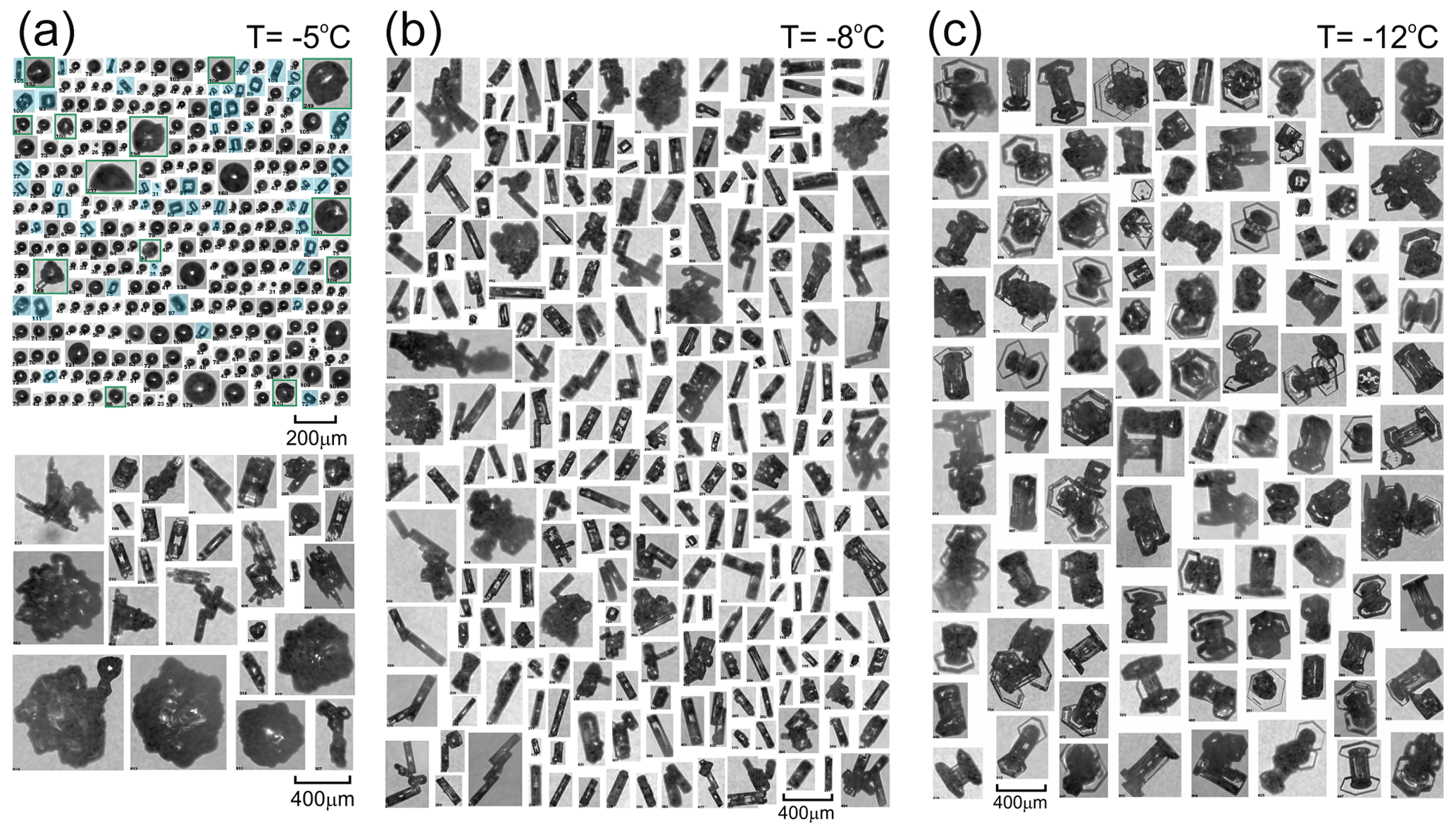
Figure 1 Images of ice particles observed in MCSs during the NRC Convair-580 flight on 15 May 2015 measured by the SPEC CPI. (a-top) Spatial sequence of liquid drops and small facetted ice crystals (highlighted by blue) and deformed and fragmented frozen drops (green frames) (for a more detailed imaging see Fig. A1 in Appendix A). (a-bottom) Large ice particles from the SIP region shown in panel (a-top) from 09:40:42–09:40:47 UTC and at 5600 m, T = −5.1 °C, IWC ≈ 0.6 g m⁻³, and N_ice ≈ 1000 L⁻¹. (b) Spatial sequence of ice particles measured in the cloud region dominated by columnar ice from 10:49:58–10:50:04 UTC at 6250 m, T = −7.8 °C, IWC ∼ 1.8 g m⁻³, and N_ice ≈ 600 L⁻¹. (c) Spatial sequence of particles in the region dominated by capped columns from 11:47:38–11:47:50 UTC at 7000 m, T = −11.7 °C, IWC ∼ 0.9 g m⁻³, and N_ice ≈ 100 L⁻¹.

2.2 Ice initiation

The mechanism behind the ice initiation is the key to understanding the formation of HIWC in tropical MCSs. One of the most striking findings of this research was the observation of unusually high amounts of small facetted ice crystals with sizes < 100 µm that formed just above the melting layer at temperatures −5 °C < T < −2 °C (Korolev et al., 2020). Typically, the observed small ice crystals were solid hexagonal prisms with aspect ratios ranging from 0.3 to 6. Examples of such small ice crystals are shown in Figs. 1a and A1. The concentration of small ice crystals ranged from 10² to 10³ L⁻¹, which exceeds the estimated concentration of ice nucleating particles (INPs) (N_INP; Ladino et al., 2017) by 6–8 orders of magnitude. Such a big difference between N_ice and N_INP suggests that the initiation of small facetted ice particles is related to SIP (Field et al., 2017).

At present, there are six recognized SIP mechanisms (Korolev and Leisner, 2020). Identification of the specific SIP mechanisms responsible for the formation of the observed ice is hindered by the essentially Eulerian nature of the observations. Such observations do not allow direct observations of SIP processes but rather enable the observation of the products of SIP after the SIP events have occurred. In this regard, the analysis of the cloudy environment associated with SIP may provide some hints about the mechanisms responsible for the enhanced ice concentration. The important condition for using such evidence is that the mechanisms may be spatially correlated with the SIP environment.

The age of the small facetted ice crystals at −5 °C is estimated as less than 2–3 min (Korolev et al., 2020). As argued in the aforementioned study, the point of origin of such young ice particles is near the location of their observation. This enables the use of the evidence found in the environment populated by small facetted ice crystals for the identification of the possible type of the SIP mechanism. Thus, it was found that in many cases the regions with enhanced concentrations of small facetted ice were associated with the presence of supercooled large drops (SLDs), and they also contained fragments of deformed and fragmented frozen droplets. Such droplets are highlighted by green frames in Fig. 1a (see also Fig. 18 in Korolev et al., 2020). Observations of precipitation size drops, fragmented and deformed frozen drops, and large concentrations of tiny facetted ice crystals suggest that the “fragmentation of freezing droplet” (FFD) SIP mechanism is responsible for the enhanced concentration of the observed ice concentration above the melting layer.

2.3 Metamorphosis of ice particle shapes

Early laboratory studies revealed that the growth rate ($\mathrm{d}L/\mathrm{d}t$) of ice particles along the crystallographic axes (i.e., a and c) is highly sensitive to humidity and ambient temperature (e.g., aufm Kampe et al., 1951; Nakaya, 1954; Kobayashi, 1957; Hallett and Mason, 1958; Ryan et al., 1976). This unique feature of ice growth results in an infinite variety of intricate ice particle shapes. However, despite the complexity and variety of ice shapes, there are two major growth regimes. The first occurs when the growth rate of the prism faces (i.e., along the c axis) exceeds the growth rate of the basal faces (i.e., along a axes) e.g., $\mathrm{d}{L}_c/\mathrm{d}t$ > $\mathrm{d}{L}_a/\mathrm{d}t$. This regime results in a formation of columnar type of ice crystals, e.g., solid and hollow columns, scroll, sheath, needles, and bullets. The second growth regime corresponds to the case when the growth rate along the c axis is slower compared to the growth rate along a axes, e.g., $\mathrm{d}{L}_c/\mathrm{d}t$ < $\mathrm{d}{L}_a/\mathrm{d}t$. This regime corresponds to the formation of planar types of ice crystals such as plates, stellar, and dendrites. The preferential growth directions of ice crystals along a and c axes change versus temperature in a cyclical way, changing the habits between plate–column–plate–column near −4, −9, and −22 °C, respectively (e.g., Kobayashi, 1961; Magono, and Lee, 1966; Rottner and Vali, 1974; Pruppacher and Klett, 1997). Temperature (T) and relative humidity (RH) experience continuous changes in a cloud environment due to the air vertical motion and mixing. This results in metamorphoses of ice particle shapes due to changes in the dominant growth direction, depending on T and RH at each moment of time. Therefore, in some special cases, observations of ice particle habits may allow the reconstruction of the history of T and RH which the ice particles had experienced. In this section, we consider ice particle habits observed in tropical MCSs, which provide information on ice particle history and their vertical travel.

One of the important features of tropical MCSs at temperatures −10 °C < T < −5 °C is that, in many cases, columnar ice is the dominant habit of particles constituting HIWC regions. The fraction of columns in HIWC regions in some cases may approach 100 %. An example of ice particle images in such a HIWC environment is shown in Fig. 1b.

The typical size of the observed columns varied from 200 to 500 µm, and their concentration changes in the range from 10² to 10³ L⁻¹. This is quite a high concentration of ice, and it cannot be explained by primary ice nucleation in the −10 °C < T < −5 °C temperature range (Ladino et al., 2017). The similarity of the concentrations of columns at −10 °C < T < −5 °C and small facetted secondary ice crystals at −5 °C < T < −2 °C and the spatial proximity in the vertical direction of these two temperature layers is indicative that the columnar ice in the HIWC cloud region is consistent with the successive growth of the secondary ice formed in the vicinity of the melting layer after their ascent in convective updrafts.

Higher up in the cloud, at the levels with T < −12 °C, it was found that the population of ice crystals in HIWC regions contained a large number of capped columns. Similar to columnar ice, in some cases the fraction of capped columns may reach nearly 100 %, as shown in Fig. 1c. Observations of capped columns in tropical MCSs were also reported by Ackerman et al. (2015; Fig. 1). Leroy et al. (2017; Fig. 8) presented measurements of ice particle images dominated by capped columns, which were sampled at −37 °C in the HIWC cloud region during the HAIC–HIWC campaign.

Capped columns are a result of the metamorphosis of columnar ice crystals after transitioning from the columnar growth regime to the plate growth regime determined by the ambient T and RH. In this case, the pre-existing columnar crystals alter their primary growth direction from the c axis direction to the a axes. However, due to higher gradients of water vapor around sharp ice edges, the crystal areas in the vicinity of the edges of the basal face will have a higher growth rate along the a axes compared to that of the rest of the prismatic faces (e.g., Nelson, 2001). This leads to the formation of plates capping the ice column ends.

The association of columns and capped columns with HIWC regions and their linkage through the metamorphosis of the ice shapes suggests that the capped columns originate from the columns formed at −10 °C < T < −5 °C. Formation of capped columns may also be associated with the metamorphosis of columns formed at high altitudes at T < −22 °C that then precipitated down to the levels with temperatures −9 °C > T > −22 °C, corresponding to the plate growth condition. Such a scenario was discussed by Heymsfield et al. (2002). This case may be also relevant to some fraction of ice crystals in the studied MCSs. However, such sequence of ice transformation cannot explain observations of capped columns at temperatures of −37 °C (Leroy et al., 2017) since it assumes that the original columns were formed at lower temperatures at a higher altitude and, upon precipitating down to the −37 °C level, they cannot experience the plate growth conditions; therefore, they cannot transform into capped columns.

Observations of capped columns at temperatures around −37 °C can be also explained by recirculation through the levels with −9 °C > T > −22 °C of the columns formed at T < −22 °C. However, such a scenario seems unlikely to explain nearly uniform population ice crystals consisting of columns and capped with large spatial extension and concentration reaching a few hundred liters (Leroy et al., 2017).

Summarizing the above, the most likely scenario for the evolution of ice particles in the convective cloud regions in tropical MCSs is as follows. Secondary ice initiation occurs in the vicinity of the melting layer in the temperature range −5 °C < T < −2 °C, resulting in the generation of numerous small facetted ice crystals Figs. 1a and A1. After an ascent within the convective updraft to the level −9 °C < T < −5 °C , the faceted small ice crystals turn into columns (Fig. 1b). A subsequent ascent though the temperature range −22 °C < T < −9 °C turns columns into capped columns (Fig. 1c). Figure 1 shows ice particles sampled in the same MCSs in convective regions but at different temperatures. Even though these images were sampled in horizontally separated regions, they support the proposed sequence of ice metamorphosis. Analysis of ice particle images HIWC regions in other studied MCSs showed the same altitude pattern of changes in the particle habits.

A conceptual diagram describing the metamorphosis of ice particles in convective regions of studies MSCs is shown in Fig. 2. It should be noted that HIWC regions frequently contain ice particles with habits different from columns or capped columns. The presence of such particles is related to the entrainment in the convective updrafts of aged ice particles with different histories from the ambient cloud regions or precipitating from above.

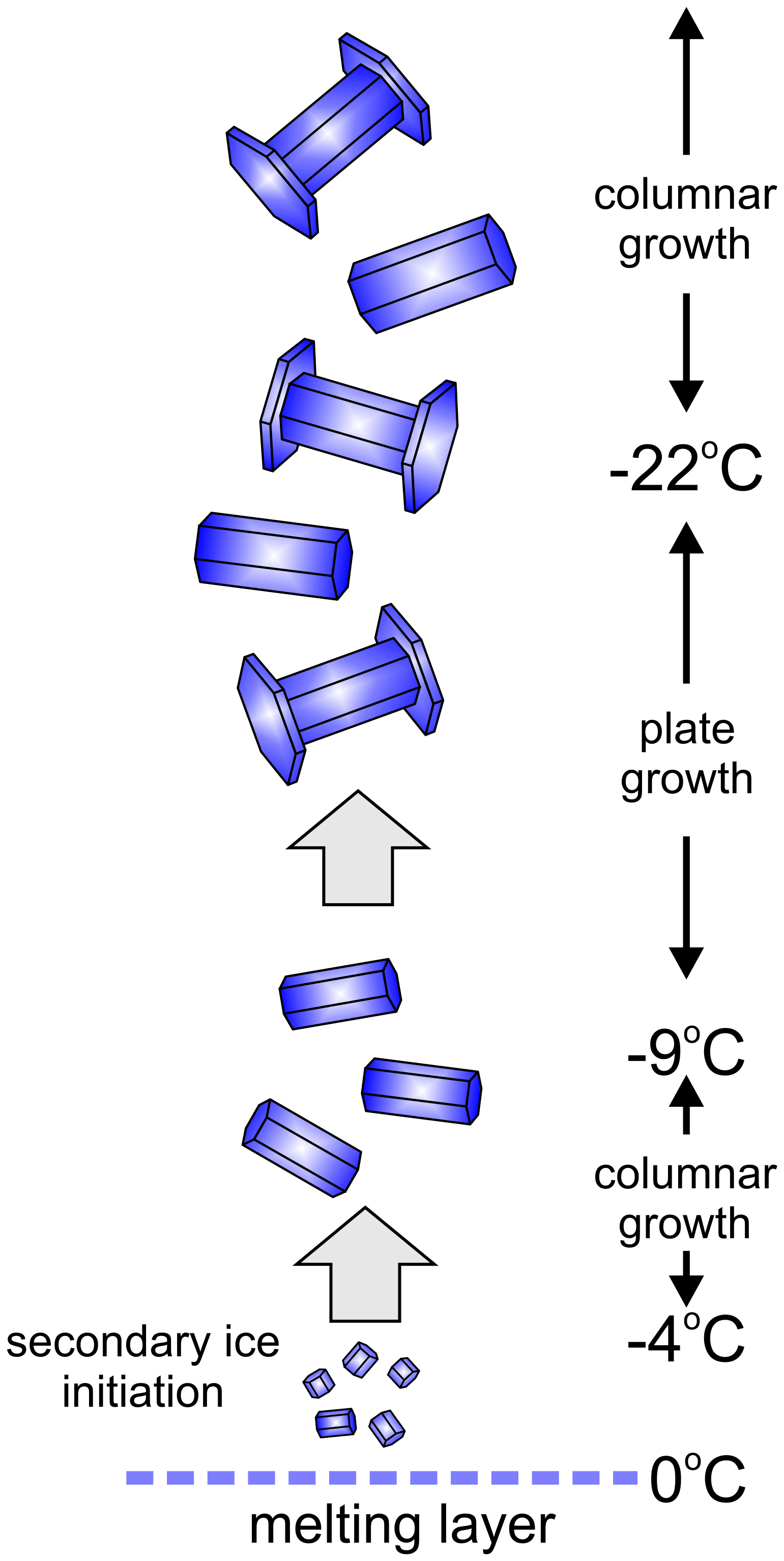
Figure 2 A conceptual diagram of metamorphosis of ice particles in convective regions in tropical MCSs.

2.4 Ice concentration, particle sizes, and IWC

Besides the shape of ice crystals, the way mass is distributed across the population of ice particles may also be exploited to retrieve the microphysical processes which the ice particles underwent. Thus, the relationship between IWC, N_ice, and particle size may provide important information about the mechanisms of HIWC formation. In the following discussion, the MMD_ice will be used as a metric of the population of ice particles.

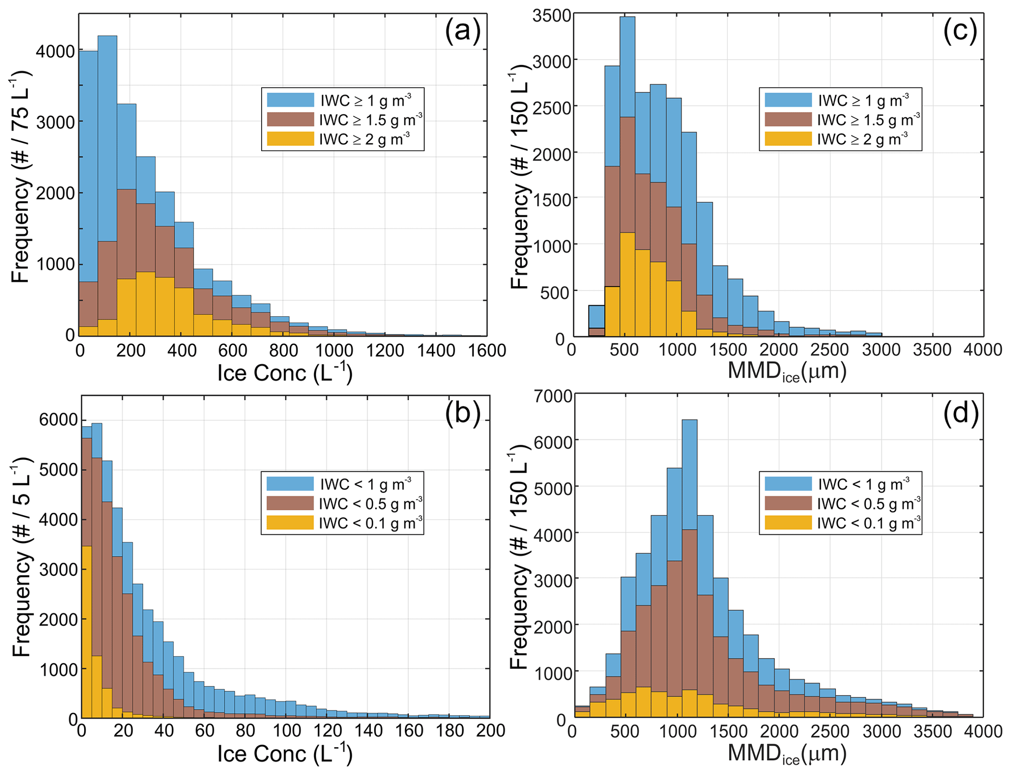
Figure 3 Probability density function of N_ice and MMD_ice in cloud regions with (a, c) IWC ≥ 1, 1.5, and 2 g m⁻³ and (b, d) IWC < 1, 0.5, and 0.1 g m⁻³, respectively. Measurements were collected in the temperature range −15 °C < T < −5 °C.

To explore IWC–N_ice and IWC–MMD_ice relationships, we employed data collected by particle imaging probes, primarily the 2D-S and PIP. To reduce the biases in calculations of N_ice due to uncertainty in the definition of the depth-of-field and diffraction effects on particle image sizing, the first three size bins in the 2D-S measurements were omitted, which resulted in PSDs and N_ice calculations for D_ice ≥ 40 µm. Such truncation is a reasonable compromise between uncertainty in concentration related to measurements of low pixel number images and underestimation of particle concentration due to disregarding small images.

An analysis of the mass distributions of ice particles shows that the particle mass concentration rapidly decreases with the decrease in the particle size for D < 200 µm. The estimated bias in calculations of MMD_ice related to uncertainty in the particle counting with D < 40 µm for the Cayenne data set is expected to not exceed 8 %.

The IWC was primarily measured by the IKP. Calculation of IWC from the IKP required accurate measurements of the background humidity. Unfortunately, in several flights the background humidity sensor was malfunctioning. Therefore, to increase the statistics of the IWC–N_ice and IWC–MMD_ice relationship, IWC was calculated from the integration of the composite PSDs measured by 2D-S and PIP. The coefficients a and b in the size-to-mass parameterization M=aL^b, where M is the particle mass, and L is the particle image maximum dimension, were found by minimizing the difference between IWC calculated from the measured PSDs and that measured by the IKP for the flights when accurate RH measurements were available (a = 7.0044 × 10⁻¹², b = 2.3). This approach was motivated by the fact that the HIWC environment was dominated by columnar ice crystals, which resulted in different coefficients a and b obtained for irregularly shaped ice particles in the original study by Brown and Francis (1995).

Figure 3a shows probability density functions (PDFs) of N_ice for ice particles with D_ice ≥ 40 µm in HIWC cloud regions with IWC ≥ 1, 1.5 and 2 g m⁻³. As already seen, the PDFs of N_ice have modal distributions with modal concentrations increasing approximately from 100 to 250 L⁻¹ with the increase in IWC. The ice concentration in HIWC cloud regions varies across a broad range, reaching maximum of 4 × 10³ L⁻¹.

Table 1 The 10th, 50th, and 90th percentiles of ice particle concentrations with D_ice ≥ 40 µm and MMD in cloud regions with different IWC in the temperature range −15 °C < T < −5 °C.

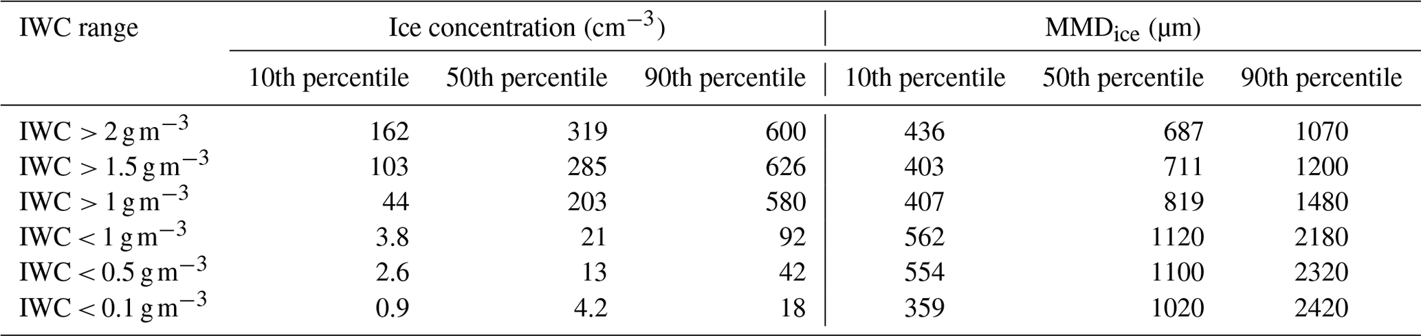
The PDFs of N_ice with IWC < 1, 0.5 and 0.1 g m⁻³ are shown in Fig. 3b. As already seen, the behaviors of N_ice PDFs in the low IWC regions contrast with those in the HIWC environments in Fig. 3a. The ice particle concentrations in low IWC clouds appear to be much smaller compared to that in HIWC regions. Comparisons of the 10th, 50th, and 90th percentiles of N_ice for low IWC and HIWC environments in Table 1 illustrate the well-pronounced difference between these low and high IWC cases.

The PDFs of MMD_ice in high and low IWC cloud regions are shown in Fig. 3c and d. As already seen, MMD_ice in HIWC cloud region cloud ice particles have smaller MMD_ice, whereas in low IWC clouds, the MMD_ice is higher. The relationships between MMD_ice and IWC can also be seen from Table 1, which shows increase in the 10th, 50th, and 90th percentiles of MMDs with the decrease in IWC.

The relationship between N_ice, MMD_ice, and IWC can be seen in more details from the scatter diagrams of N_ice(IWC) and MMD_ice(IWC) in Fig. 4a and b. As shown in Fig. 4a, the median N_ice increases monotonically with the increase in IWC up to 2 g m⁻³ and then remains approximately constant and equal to 320 L⁻¹. However, MMD_ice has a general tendency to decrease with increases in IWC (Fig. 4b).

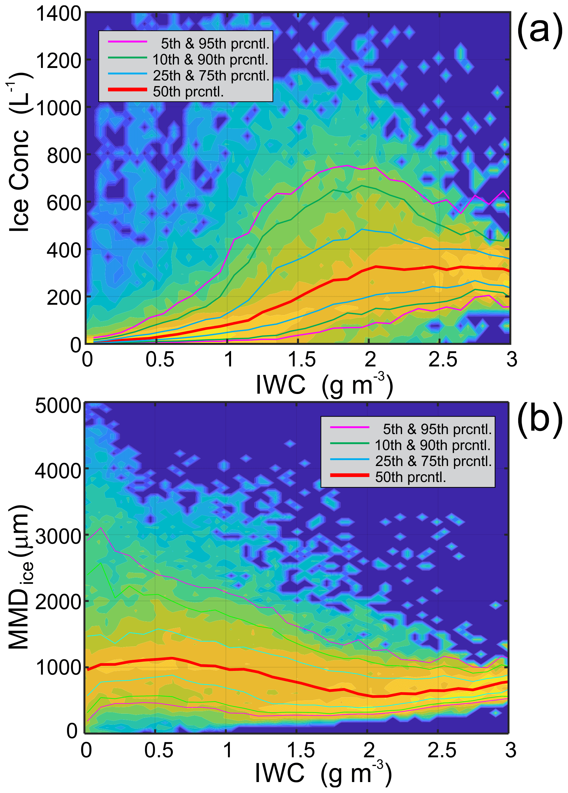
Figure 4 Scatter diagram (a) N_ice vs. IWC and (b) MMD_ice vs. IWC at −15 °C < T < −5 °C. In the density map, the PDFs of N_ice and MMD_ice were normalized on unity at each interval ΔIWC = 0.05 g m⁻³ in the temperature range −15 °C < T < −5 °C.

The main conclusion from Figs. 3 and 4 is that despite a large scatter of N_ice and MMD_ice vs. IWC, HIWC environments at −15 °C < T < 5 °C mainly consist of a relatively high concentrations of small ice particles, with the median values of N_ice ranging from 200 to 300 L⁻¹ and median MMD_ice ranging between approximately 700 and 800 µm (Table 1). However, in low IWC clouds, most cases have a relatively low N_ice with median values of less than 20 L⁻¹ and median MMD_ice exceeding 1000 µm. As was shown in Hu et al. (2021), the correlation between N_ice and IWC remains down to the −50 °C < T < −40 °C temperature range.

There are two possible explanations for the observed relationship between N_ice and IWC. First, ice particles could be initiated at the upper parts of the MCSs through homogeneous (e.g., at T < −40 °C) or heterogeneous (at T > −40 °C) freezing of cloud droplets in convective updrafts. The amount of generated ice may be sufficient to explain the observed concentrations of ice particles. The drawback of this explanation is that the shape of ice particles formed on frozen droplets at low temperatures is dominated by bullet rosettes (e.g., Bailey and Hallett, 2009). However, this type of ice particle habit was not observed in any noticeable amount in the studied MCSs. This makes this explanation less plausible.

The second explanation is related to ice initiation through SIP processes above the melting layer, where secondary ice particles are then transported to the upper parts of the MCSs by convective updrafts. This explanation is consistent with the observed ice particle habits, as discussed in Sect. 2.3.

2.5 Mixed-phase cloud regions

The analysis of the data collected from the NRC CV580 showed that in mature MCSs mixed-phase environments are quite sparse. The spatial occurrence of mixed-phase regions averaged over the entire data set at −2 °C > T > −15 °C was 4.8 %. Mixed-phase cloud was observed in spatially small-scale regions, with the mean and median horizontal extension of 0.48 and 0.23 km, respectively, and the maximum length of 2.5 km. Nearly all observed mixed-phase cloud regions were associated with vertical updrafts exceeding 1 m s⁻¹. However, many strong updrafts with u_z ∼ 10 m s⁻¹ contained no liquid. Average and median LWC observed in mixed-phase regions was 0.047 and 0.034 g m⁻³, with the maximum LWC peaking up to 0.1 g m⁻³. For most of the observed mixed-phase cases, LWC ≪ IWC, with an average liquid water fraction $\mathrm{LWC}/\mathrm{TWC}$ = 0.13. These results are generally consistent with the data collected from the SAFIRE F20 (Strapp et al., 2021). The F20 data showed 0.2 % of spatial occurrence mixed phase at −30 °C and no presence of liquid below −35 °C. Earlier, a similar conclusion about trace amounts of liquid water in tropical MCSs was obtained in Lawson et al. (1998).

The low occurrence and sparsity of mixed phase in MCSs is consistent with the observation of high concentration of ice in HIWC regions, which creates conditions favorable for rapid glaciation of clouds. Thus, for a still air U_z = 0 m s⁻¹, initial LWC₀ = 0.1 g m⁻³, temperature T = −5 °C, ice particle size L_i = 100 µm, and concentration N_i = 300 L⁻¹, the mixed-phase cloud will glaciate due to the Wegener–Bergeron–Findeisen process within 120 s (Korolev and Isaac, 2003). The riming process will expedite the conversion of liquid into ice, and the glaciation time will be even shorter.

Besides the concentration of ice, the glaciation time also depends on the vertical velocity and the initial LWC (Korolev and Isaac, 2003; Pinsky et al., 2014). Since the droplets and ice may grow simultaneously (Korolev and Mazin, 2003), the glaciation process may take longer, or the cloud may glaciate after reaching the homogeneous freezing temperature. Therefore, the mixed-phase cloud may exist only in a horizontally narrow regions associated with convective updrafts. Analysis of the X- and W-band radar Doppler velocities showed that the typical horizontal dimensions of the updrafts are a few hundred meters. This is consistent with the typical spatial horizontal scale of mixed-phase clouds in MCSs.

2.6 Sparse supercooled large drops

One of the interesting features related to mixed-phase regions is the observation of SLDs, with D ranging from 50 to 200 µm embedded in ice clouds with no presence of small droplets. An example of spatially sparse large drops is shown in Fig. 5 (red frames).

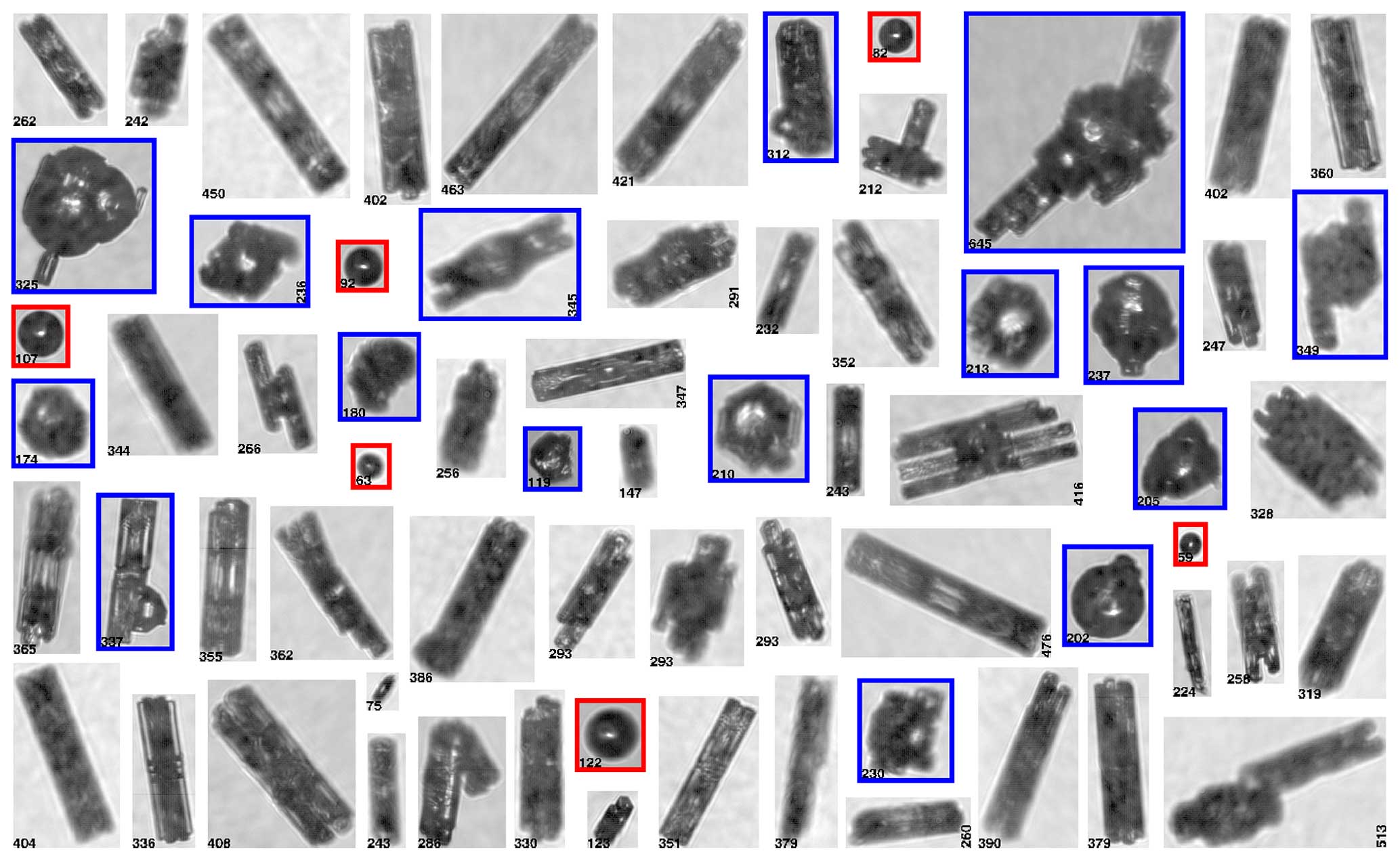
Figure 5 Spatial sequence of cloud particle images measured by the CPI with isolated large drops (red frames) embedded in the ice environment shown in Fig. 6. Blue frames indicate ice particles with attached or embedded large frozen drops. Numbers inside the image frames indicate the maximum size of the particle images in micrometers. H = 6500 m, T = −9.5 °C, 10:48:10–10:48:11 UTC on 26 May 2015.

Identification of “sparse” SLD regions in tropical MCSs with the help of OAPs (e.g., 2D-S, CPI, and 2DC) and scattering probes (e.g., FSSP and CDP) is hindered due to the limitations of their performances. Thus, scattering probes do not respond in sparse SLD regions since, in most cases, the diameters of the smallest drops there exceed the maximum measured size of these instruments. On the other hand, OAP images of out-of-focus small ice crystals, in many cases, appear as the out-of-focus images of drops, and therefore, images of ice particles may be confused with liquid drops.

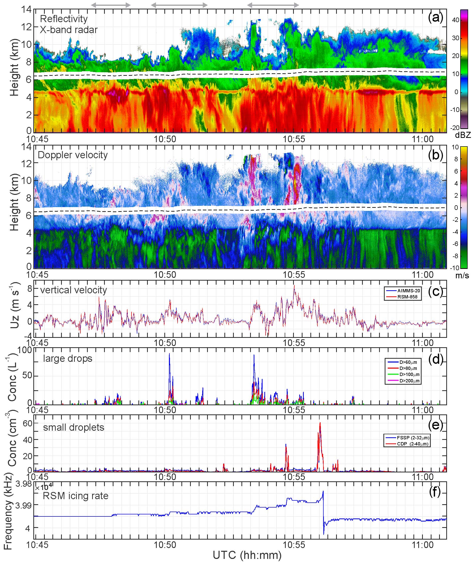
Figure 6 Time series of (a) X-band radar reflectivity, (b) Doppler velocity measured by X-band radar, (c) AIMMS-20 and Rosemount 858 vertical wind velocity, (d) SLD number concentration estimated from CPI measurements, (e) FSSP and CDP concentration, and (f) Rosemount icing detector frequency. The three arrows at the top indicate cloud regions with an elevated bright band. The measurements were collected at 6500 m < H < 7000 m and −12 °C < T < −9.5 °C on 26 May 2015. GOES-13 satellite images with the Convair-580 flight track for this flight segment are shown in Fig. B1a and b.

In this study, the detection of sparse SLDs was identified from the CPI high-resolution imaging probe with the help of the image-processing software trained on the ensemble of droplet images collected in warm clouds. Even though the CPI is not well qualified to measure bulk microphysical parameters, it allows for a crude estimate of the number concentration, which is sufficient for this study. Assessment of the number concentration based on Connolly et al. (2007) showed that the droplet concentration in sparse SLD regions varied in a wide range with a maximum of the order 10² L⁻¹. The estimate of the minimum local droplet concentration depends on the spatial averaging scale, and it may go well below 10⁻³ L⁻¹.

Figure 6d shows a time series of the SLD concentration with drop diameters larger than 60, 80, 100, and 200 µm. As can be seen, sparse SLD regions were usually observed in convective updrafts and their vicinity (Fig. 6b and c). In many cases in tropical MCSs, SLD regions (Fig. 6d) are spatially separated from cloud regions with small droplets measured by scattering probes (Fig. 6e).

Strictly speaking, the identification of the thermodynamic phase of spherical particles from their images at T < 0 °C is ambiguous since the images of liquid and freshly frozen non-deformed drops appear the same way. However, the response of RID in the sparse SLD regions (Fig. 6f) unambiguously indicates that at least some fraction of the spherical particles in the CPI imagery is in the liquid phase. Based on the rate of changes in the RID signal (Mazin et al., 2001), it was found that in SLD regions at 2 km above the melting layer, LWC may reach over 0.1 g m⁻³. It is worth mentioning that there were multiple episodes of airframe icing experienced by the CV580 in the SLD regions during operations in tropical MCSs, two of which resulted in occasions of buffeting (Anthony Brown, NRC pilot, personal communication, 2015).

A conventional explanation for large drops consists of attributing their formation to the collision–coalescence process. Such an explanation assumes the presence of small droplets to enable the growth of larger drops due to coalescence with smaller ones. The presence of small droplets will also lead to the formation of rimed ice particles. Rimed ice can be easily identified from the high-resolution imagery based on the distinct features on ice particle surfaces. However, no small-droplet riming was found within hundreds of meters around regions with sparse SLDs. Instead, there were many large (50–200 µm) frozen drops on the surfaces of ice particles or regrown in ice crystals (blue frames in Fig. 5). This is suggestive that the collision–coalescence process was unlikely to have a significant contribution to the formation of sparse SLDs.

An alternative explanation of the sparse large drops is related to their uplift through the melting layer. This hypothesis is supported by the absence of small droplet riming and the observation of large frozen drops inside or attached to ice particles (Fig. 5; blue frames). The terminal fall velocity of a 200 µm drop at the level of the melting layers is approximately 1 m s⁻¹. Therefore, these drops could be transported by a moderate convective updraft (e.g., 4–5 m s⁻¹) from the melting layer to the level of the observations (ΔH ∼ 1 km) within 5–6 min.

2.7 Disturbance of the bright band

Another interesting feature observed during the HAIC–HIWC field campaign is a disturbance of the top of the bright band. Figure 6a shows one of the examples of the bright band patterns measured by the X-band radar during transit through the MCSs on 26 May 2015 (Fig. B1a and b). As seen in Fig. 6a, the top of the bright band was relatively uniform in stratiform regions where at the flight level the vertical wind velocity U_z is close to 0 m s⁻¹ (Fig. 6c) (time segments include 10:44:40–10:46:30, 10:52:10–10:53:10, and 10:58:20–11:01:00 UTC). However, in convective regions, the enhanced reflectivity above the level of the undisturbed bright band may extend up to 1.5–2 km. This can be seen from the diagrams with the vertical Doppler velocity (Fig. 6b) and vertical wind velocity U_z at the flight level (Fig. 6c), which correspond to the convective regions within the time segments 10:47:05–10:48:40, 10:49:25–10:51:20, and 10:53:10–10:55:15 UTC (indicated by arrows in Fig. 6a).

The bright band forms as a result of the enhanced radar return from melting ice particles falling below the freezing level. The linkage between the bright band and freezing level suggests that the spatial vertical fluctuations in the bright band may be explained by the vertical fluctuations in the 0 °C isotherm. However, 1.5–2 km vertical changes in the altitude of the freezing level would result in spatial fluctuations in the temperature, ΔT, of the order of 9 to 12 °C, with the assumption of a moist adiabatic lapse rate. Such temperature fluctuations are overly high and were never observed on kilometer spatial scales. Typically, during leveled flights in convective regions in studied MCSs, the amplitude of temperature fluctuations did not exceed ± 1 °C.

A potential explanation of the disturbance of the bright band in convective regions is related to the recirculation of completely and partially melted ice through the melting layer. The precipitation size drops formed after the melting of ice particles may be transported above the melting layer with updrafts generated by regular convection or gravity waves. Above the melting layer, SLDs will interact with the preexisting ice and thus produce high-density spherical particles and graupel which, together with SLDs, will result in the enhancement of reflectivity.

The above explanation of the enhanced reflectivity over the melting layer is consistent with the observation of SLDs (Sect. 2.6). It is also supported by positive Doppler velocity observed below and within the melting layer as in Fig. 6b (10:49:11–10:49:40, 10:52:50–10:53:20, and 10:56:02–10:56:12 UTC). It is worth mentioning that the radar average Doppler velocity has a higher sensitivity to larger drops. Therefore, even though the average Doppler velocity is negative, small droplets driven by updrafts may have a positive vertical velocity.

2.8 High IWC cloud regions and vertical updrafts

Observations collected during the HAIC–HIWC campaign showed that traversing through convective updrafts was usually accompanied by an increase in IWC over 1 g m⁻³. Nearly all convective regions with u_z > 2 m s⁻¹ observed during the Cayenne campaign were associated with enhanced IWC. The HIWC regions around convective updrafts extended from a few hundreds of meters to tens of kilometers. A detailed study of the statistics of horizontal spatial scales of HIWC cloud regions is available from Strapp et al. (2021). However, in some cases, no convective updrafts were observed during transit through the HIWC regions.

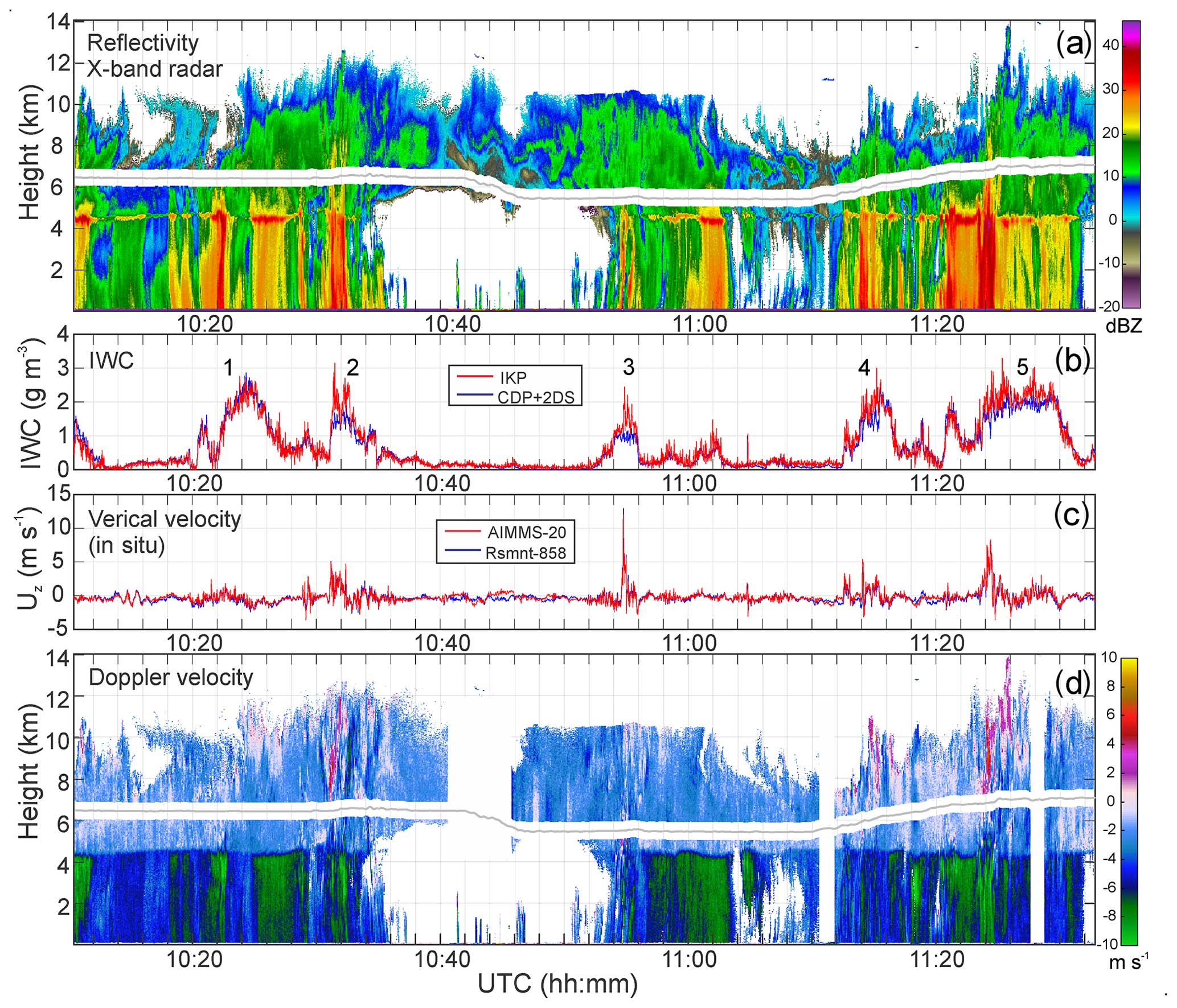
Figure 7 Time series of (a) X-band radar reflectivity, (b) IWC, (c) vertical velocity, and (d) Doppler velocity measured by the X-band radar. The numbers in panel (b) indicate HIWC cell number (see the text). The measurements were collected from the NRC Convair-580 on 27 May 2015. GOES-13 satellite images with the Convair-580 flight track for this flight segment are shown in Fig. B1c and d.

The time series in Fig. 7 illustrates the relationship between IWC and u_z described above (Appendix B). As already seen, four of five HIWC cells (i.e., nos.2–5 in Fig. 7b) are associated with the embedded convection observed somewhere within these cells (Fig. 7c). In situ vertical velocity measured on the flight level (Fig. 7c) correlates well with the Doppler velocity (Fig. 7d), which in some cases may extend to the cloud top of the MCSs. However, no distinct convective updrafts were observed within HIWC cell no. 1 (in Fig. 7b; ∼ 10:20–10:26 UTC). An encounter of the convective updrafts during the transit through the HIWC region depends on the flight pattern, and it is possible that the aircraft trajectory did not intersect or come close enough to the convective region. It is also possible that during sampling of the HIWC region, the convection in this area faded away.

A comprehensive analysis of the relation between IWC and the proximity to the center of the nearest convection based on the combined analysis of the in situ and satellite data was conducted by Hu et al. (2021). It was found that IWC, on average, depends on the distance from the convective core (L_conv) and that IWC decreases with increasing L_conv. The dependence of IWC on the distance from the convective core was also indicated in Lawson et al. (1998).

The relationship between IWC and U_z described above suggests that the convective updrafts transport small ice particles to the upper levels. Due to the small fall velocity, newly formed secondary ice particles can be transported to high altitudes even with a relatively low vertical velocity. During the ascent, ice crystals grow through water vapor deposition, which ultimately results in the formation of HIWC.

3 Numerical simulations

The objective of this section is to summarize results of numerical simulations of HIWC in tropical MCSs and explore the role of SIP in the vicinity of the melting layer on the formation of HIWC environments.

3.1 Model configuration

3.1.1 Atmospheric model

The numerical model used in this study is the Global Environmental Multiscale (GEM) atmospheric model (Côté et al., 1998; Girard et al., 2014). GEM is the operational numerical weather prediction (NWP) model of Environment and Climate Change Canada (ECCC) that is used for all of the ECCC's deterministic and ensemble NWP prediction systems. It is also capable of running at a high spatial resolution (including sub-kilometer and near-cloud-resolving scales) for detailed atmospheric research purposes. The dynamical core of GEM is formulated based on the non-hydrostatic, fully compressible, and primitive equations with a terrain-following hybrid vertical grid. For the simulations described below, the model dynamics and physics options are summarized in Appendix C (Table C1).

A tropical MSC that was observed during the HIWC–HAIC campaign was simulated using a quasi-idealized model configuration of GEM, similar to the simulations described in Qu et al. (2022). A model sounding from the analysis of ECCC's global deterministic NWP system was used to initialize GEM on a domain with a 250 m horizontal grid spacing, with 256 km × 256 km and 183 unevenly spaced vertical levels. The initial atmospheric conditions were horizontally homogeneous, based on the sounding taken at 12:00 UTC on 15 May 2015 at 6.769° N and 49.551° W (Appendix C; Fig. C1). The initial sea surface temperature was set to 300.37 K. To initiate the convection, the updraft nudging method of Naylor and Gilmore (2012) was used to force convection during the first 15 min of the simulation, with a maximum vertical wind speed of 10 m s⁻¹. Three distinct updrafts 16 km apart from each other in the western part of the simulation domain were initialized. The simulations were integrated for 3 h.

In order to examine the impact of SIP on HIWC from a modeling point of view, two simulations were run. In the baseline (i.e., control) simulation, referred to BASE, four ice categories in the microphysics scheme (see Sect. 3.1.2 below) were used, and all SIP processes were deactivated. In the second run, referred to as SIP-ON, the parameterized HM and FFD mechanisms for SIP were activated (see Sect. 3.1.3 below). A comparison of the two simulations allows for an investigation of the impacts of SIP processes on HIWC.

Note that at 250 m, the simulations conducted are near to what is conventionally regarded as the “cloud-resolving” or large eddy simulation (LES) scale (with horizontal grid spacings of ∼ 100 m or less). At this scale, a 3D turbulence parameterization should be used. GEM currently lacks the capability to run in true LES mode; thus, the following results are not truly cloud-resolving simulations. However, GEM has been used successfully by other groups to simulate deep convection with a 250 m horizontal grid spacing (e.g., Belair et al., 2018). Furthermore, the model results shown below are reasonably close to the in situ observations in terms of bulk microphysical fields and the model sensitivity with respect to the inclusion of SIP processes is consistent with observational evidence. Hence, despite the limitations of the model, the simulation results can be used with a sufficient degree of confidence to support the conceptual model proposed in Sect. 4.

3.1.2 Microphysics scheme

Given the relative importance of the model microphysics in this study, some additional detail on the P3 microphysics scheme is warranted. The P3 scheme was introduced in Morrison and Milbrandt (2015). Since its inception, there have been several major developments which are summarized in Cholette et al. (2023). The liquid phase component of P3 uses a standard two-moment, two-category approach, with liquid hydrometeors partitioned into “cloud” (small droplets) and “rain”. Each liquid category is represented by a complete gamma size distribution and has prognostic variables for the mass and number mixing ratios. As such, the size distribution of each category goes from zero to infinity; however, for practical purposes, a diameter of around 80 µm can be regarded as a de facto demarcation size between the two categories.

The ice phase, on the other hand, is treated much differently in P3 than in traditional schemes which typically partition frozen hydrometeors into several predefined categories (e.g., pristine “ice”, “snow”, and “graupel”) with associated fixed parameters to prescribe physical properties (e.g., density). Rather, P3 has a user-specified number of generic ice-phase (or mixed-phase) hydrometeor categories, each of whose physical properties can evolve freely and continuously in time and space due to the choice of prognostic variables (Milbrandt and Morrison, 2016). The PSD for each ice category is a complete gamma function. The following six mixing ratio variables for each ice category are predicted: the total mass, rime mass, liquid mass, total number, rime volume, and the sixth moment. With these prognostic variables, which are advected by the GEM dynamics and whose values are updated due to microphysical process in the P3 scheme itself, bulk physical properties (of each ice category), including density, mean size, rime fraction, liquid fraction (thereby allowing for mixed-phase particles), and PSD spectral width, are all predicted independently. Fields such as bulk fall speeds and radar reflectivity can also be computed and benefit from the degrees of freedom.

While each ice category is generic and can represent a wide range of mixed-phase hydrometeor particles, it can only represent a single dominant mode or particle type (e.g., lightly rimed small aggregates) for the population of particles that it represents. In order to represent multiple modes of ice particles at a given point in space (i.e., model grid point) and time, two or more ice categories must be used. Thus, in order to model SIP using P3, at least two ice categories must be used since SIP can result in the production of numerous small crystals in the presence of pre-existing larger ice, such as graupel in the case of the HM SIP process. The P3 microphysics scheme, therefore, is an appropriate and useful tool for the examination of the impacts of SIP in an atmospheric model. Qu et al. (2022) showed a “near-convergence” of GEM model solutions with P3 using three ice categories. In the simulations in this study, four ice categories were used.

The Doppler velocities were calculated offline by subtracting the mass-weighted fall speed of hydrometeors from the vertical wind speed. In the P3 scheme, the mass-weighted fall speed for each ice category is computed based on the fall speed for an individual particle of a given size and set of predicted bulk properties (following Heymsfield et al., 2007) and integrated over the particle size distribution (see Morrison and Milbrandt, 2015, for details). The overall mass-weighted fall speed is then obtained by summing the bulk fall speeds of all four ice categories and for rain, weighted by their respective masses.

3.1.3 Parameterization of SIP processes

Two SIP mechanisms were examined, HM and FFD, and are activated in the SIP-ON simulation. The parameterized HM process produces 10 µm ice splinters with a maximum number of 350 crystals per milligram of collected liquid cloud droplets by graupel during riming within a temperature range of −3 °C > T > −8 °C, with the peak value at −5 °C and varying linearly to zero at the extreme temperature ranges. In the P3 scheme, ice properties evolve freely within a free-ice category, as there is no predefined graupel category. For this study, graupel is defined as ice with a rime fraction between 0.4 and 1.0, a bulk ice density between 50 and 700 kg m⁻³, and a mean mass diameter greater than 2 mm.

For FFD, the number of ice splinters produced is calculated based on the number of raindrops with diameters between 100 and 3500 µm colliding with ice particles with diameter smaller than 100 µm. This parameterized process follows the heuristic relationship proposed by Lawson et al. (2015), based on the agreement of parcel model results with in situ aircraft observations:

$$\begin{array}{}\text{(1)}& N_{\text{sip}}=N_{\mathrm{r}}\mathrm{2.5}\times {\mathrm{10}}^{-\mathrm{11}}{D}^{\mathrm{4}},\end{array}$$

where N_sip is the number of ice splinters produced by the freezing of raindrops of a given diameter D. N_r is the number of drops with diameter D colliding with ice particles with diameter smaller than 100 µm. The total number of ice splinters produced by FFD process will be the integral of Eq. (1) over D between 100 and 3500 µm. To prevent extreme values of the ice number mixing ratio, a maximum total value of 5 × 10⁷ kg⁻¹ (the sum of all four ice categories) is imposed in the simulations.

Based on Keinert et al. (2020), the FFD process exhibit activity within a specific temperature range of −25 °C < T < −2 °C. Their findings indicate that among supercooled liquid drops, the most frequent splitting and ejection events occur at −12.5 °C. However, the dependence of the total number of small ice splinters versus temperature and drop size remains unclear from laboratory studies to date. The observational evidence suggests that SIP production is particularly active within 2 km above the melting layer. In this study, the maximum FFD rate N_sip is set to occur at T = −4 °C. Beyond this point, the FFD rate is assumed to decrease linearly from its peak at −4 °C to zero at the two temperature extremes (−25 and −2 °C).

In the analysis in the following sections, various quantities are computed from direct model output fields from the GEM simulations. The raw model output fields include mixing ratios for hydrometeor mass and total number for cloud droplets (Q_c and N_c), rain (Q_r and N_r), and each category x for ice (Q_i,x and N_i,x). For Q_i,x, this is the total (for category x) of the deposition mass, rime mass, and liquid mass (for mixed-phase particles), each of which are independent prognostic model variables. With the air density ρ_a, the mass contents are computed as LWC_cloud = ρ_aQ_c, LWC_rain = ρ_aQ_r, and IWC = ${\mathit{\rho }}_{\mathrm{a}}(Q_{\mathrm{i},\mathrm{1}}+Q_{\mathrm{i},\mathrm{2}}+Q_{\mathrm{i},\mathrm{3}}+Q_{\mathrm{i},\mathrm{4}})$, and the total number concentrations as N_cloud = ρ_aN_c, N_rain = ρ_aN_r, and N_ice = ${\mathit{\rho }}_{\mathrm{a}}(N_{\mathrm{i},\mathrm{1}}+N_{\mathrm{i},\mathrm{2}}+N_{\mathrm{i},\mathrm{3}}+N_{\mathrm{i},\mathrm{4}}$). However, for consistency with the observations, which exclude ice particle sizes smaller than 40 µm, each N_i,x was re-computed from the ice PSDs as the incomplete integral from 40 µm to infinity. The mean mass particle sizes were computed as D_3  cloud = $(\frac{\mathrm{6}}{\mathit{\pi }{\mathit{\rho }}_{\mathrm{w}}}\frac{{\mathrm{LWC}}_{\mathrm{cloud}}}{N_{\text{cloud}}}{)}^{\mathrm{1}/\mathrm{3}}$, D_3  rain = $(\frac{\mathrm{6}}{\mathit{\pi }{\mathit{\rho }}_{\mathrm{w}}}\frac{{\mathrm{LWC}}_{\mathrm{rain}}}{N_{\text{rain}}}{)}^{\mathrm{1}/\mathrm{3}}$, and D_3  ice = $(\frac{\mathrm{6}}{\mathit{\pi }{\mathit{\rho }}_{\text{ice}}}\frac{IWC}{N_{\text{ice}}}{)}^{\mathrm{1}/\mathrm{3}}$, where ρ_w and ρ_ice are the bulk densities of water and ice, respectively. Note that D_3  ice represents the diameter of an equivalent mass sphere. In P3, ρ_ice is a predicted variable (for each category); however, since we primarily examine small unrimed ice, a value of 917 kg m⁻³ is assumed for simplicity. The model reflectivity, Z, is computed in-line (within the microphysics scheme); see Cholette et al. (2023) for details. The total SIP rates ($\mathrm{d}{N}_{\text{ice}}/\mathrm{d}t$) are computed in-line and output for analysis.

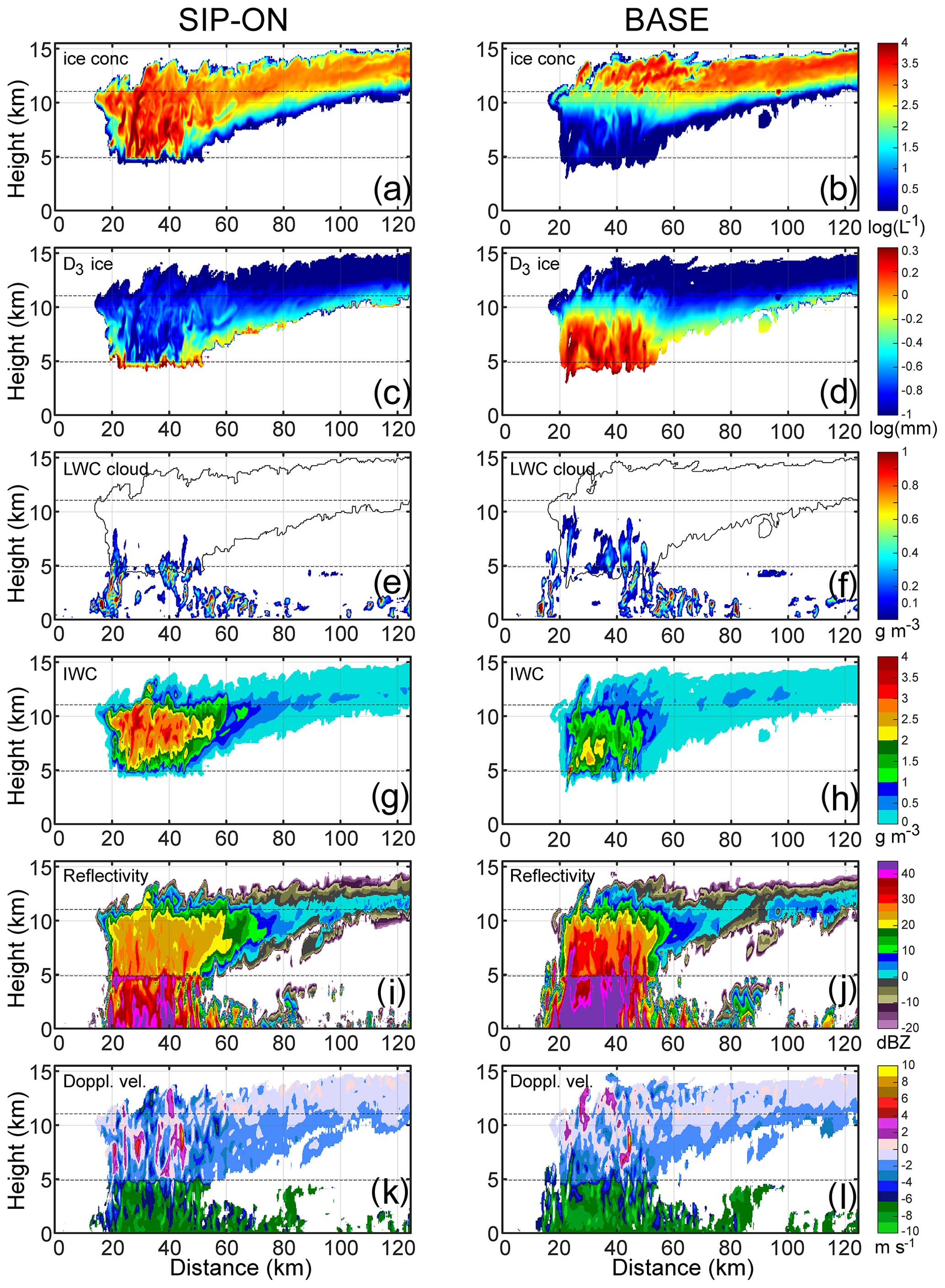
Figure 8 Vertical cross section domains of different parameters of GEM simulations for SIP-ON (left column) and BASE (right column) setups. (a, b) N_ice; (c, d) D_3  ice; (e, f) LWC_cloud; (g, h) IWC; (i, j) Z ; (k, l) U_Doppl. The cross sections were performed for the same vertical plane at 90 min on the modeled time. Horizontal dashed lines show levels corresponding to T = 0 °C (H = 4.9 km) and T = −40 °C (H = 11.1 km) levels.

3.2 Comparisons of SIP-ON and BASE simulations

The two sets of vertical cross sections of SIP-ON and BASE in Fig. 8 show stark differences between the model fields of the SIP-ON and BASE simulations. To facilitate comparison, both SIP-ON and BASE cross sections were produced along the same vertical planes at 90 min simulation time. The top view of the location of the cross sections within the cloud domain is shown in Fig. D1 (Appendix D).

In the BASE simulation, N_ice increases by approximately 2 orders of magnitude within a short distance above an altitude of 10 km (Fig. 8b). A similar rapid vertical change in ice particle sizes is seen above H ∼ 10 km, where D_3  ice decreases from approximately 1–1.5 mm at H < 10 km to 100–400 µm at H > 10 km (Fig. 8d).

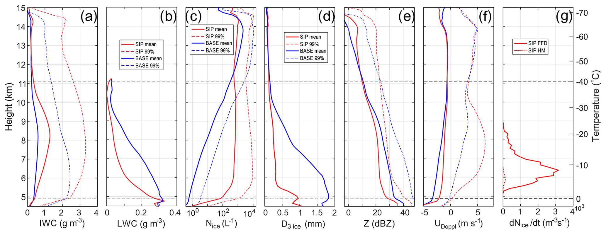
Figure 9 Average profiles of the results of SIP-ON (red) and BASE (blue) simulations. (a) IWC (solid) and IWC₉₉ (dashed); (b) LWC (solid); (c) N_ice (solid) and N_ice  99 (dashed); (d) D_3  ice; (e) Z (solid) and Z₉₉ (dashed); (f) U_Doppl (solid) and U_{Doppl  99} (dashed); (g) ice crystal production rates for FFD (solid) and HM (dashed) for the SIP-ON simulation. The profiles are spatially averaged over the cloud domain above the precipitation below the melting layer. The cloud domain was determined as the environment with IWC > 0.001 g m⁻³. The temporal averaging was performed over 13 modeling domains with time step of 5 min within the time frame from 75 to 135 min. Horizontal dashed lines show levels corresponding to T=0 °C (H=4.9 km) and $T=-\mathrm{40}$ °C (H=11.1 km) levels.

The vertical behavior of N_ice and D_3  ice in BASE is in contrast with that in the SIP-ON simulation. As seen from Fig. 8a and c, N_ice and D_3  ice experience only modest changes in the vertical direction, and they change in a smaller range compared to the BASE run. In the SIP-ON simulation, ice with high concentrations (∼ 10³ L⁻¹) is present in the cloud domain right above the melting layer (∼ 5 km), and the field of N_ice remains relatively uniform up to the cloud top (Fig. 8a). Ice particle size D_3  ice, on average, exhibits relatively minor changes between the melting layer and the cloud top (Fig. 8c). The LWC_cloud field has a broader horizontal extent (at least in most locations) and extends higher in BASE compared to the SIP-ON simulation (Fig. 8e and f). Figure 8g and h shows that the SIP-ON simulation has much higher values of IWC than BASE. Maximum IWC in the SIP-ON run approaches 4 g m⁻³ in some regions (Fig. 8g), whereas in BASE, the maximum IWC barely reaches 2.5 g m⁻³ (Fig. 8h). The area with high IWC (> 1 g m⁻³) in SIP-ON (Fig. 8g) has considerably more horizontal and vertical extent compared to BASE (Fig. 8h). Figure 8i and j show that the radar reflectivity is noticeably lower in the SIP-ON simulation than in the BASE simulation. Such behavior of Z is the reverse of that of IWC. The domains of the Doppler velocity (Fig. 8k and l) show that SIP-ON clouds are more dynamically active than those in BASE. The pattern of the Doppler velocity field in Fig. 8k also indicates significant transport of hydrometeors from the melting layer to the cloud top in the SIP-ON simulation. The intense dynamics and vertical transport of ice will stimulate vertical mixing and homogenizing fields of N_ice and IWC in the SIP-ON simulation (Fig. 8a).

While Fig. 8 provides a qualitative comparison of the results of the SIP-ON and BASE runs, a more definitive comparison of the two simulations can be examined through the temporal and spatial averaging of the modeling results, as shown in Fig. 9. The temporal averaging was done over 1 h, from 75 to 135 min of the model cloud lifetime, which includes 13 modeling domains separated by 5 min. The spatial averaging was computed over the area of precipitation. The selection of the averaging domain above the melting layer was aimed at excluding the outflow anvil area, which may extend to large distances from the convective region and is significantly affected by entrainment and mixing. Another reason for the choice of averaging was to mitigate biases when comparing with in situ airborne observations, which were collected mainly in the vicinity of the convective parts of the MCSs.

Figure 9a shows that below 11 km, the mean IWC in the SIP-ON simulation is up to 2 times higher than that of BASE. However, at H > 11 km, the average IWC in the SIP-ON and BASE simulations is approximately equal. The 99th percentile IWC₉₉ in SIP-ON remains systematically higher from the melting layer up to the cloud top. The maximum of the mean IWC occurs between 8 and 9 km. LWC in BASE remains consistently higher than that of SIP-ON between the melting and homogeneous freezing levels (Fig. 9b).

As seen from Fig. 9c, the behavior of N_ice is very different between the two simulations. In the SIP-ON run, the mean N_ice increases up to ∼ 500 L⁻¹ in the first kilometer above the freezing level and then remains moderately constant, varying between 500 and 700 L⁻¹ up to the homogeneous freezing level (∼ 11 km). After the minimum at 11.5 km, N_ice reaches a maximum of ∼ 1000 L⁻¹ above 14 km.

The vertical distribution of N_ice in BASE contrasts with the SIP-ON simulation. In the BASE run, N_ice increases monotonically with altitude, following a nearly exponential law, and its values change from ∼ 0.5 L⁻¹ at the freezing level to ∼ 2200 L⁻¹ at an elevation of approximately 14 km. The rapid increase in N_ice from 100 to 2000 L⁻¹ between 10 and 13.7 km occurs due to the homogeneous freezing of cloud droplets in convective updrafts. As seen from Fig. 9b in both SIP-ON and BASE, convective updrafts are capable of maintaining liquid water up to the homogeneous freezing level. This results in an enhancement of N_ice through the freezing of cloud droplets. The fact that the BASE N_ice becomes larger than in SIP-ON above 11.5 km is explained by the larger number of cloud droplets transported by convection to the homogeneous freezing level in BASE compared to SIP-ON, which turn into ice and enhance the ice concentration rather than evaporate due to the Wegener–Bergeron–Findeisen (WBF) process. This can also be seen in Fig. 9b, which shows a larger LWC in BASE above 11 km compared to the SIP-ON.

Figure 9d shows profiles of mean mass diameter D_3  ice. As seen in both BASE and SIP-ON, D_3  ice decreases monotonically with increasing height up to 11 km, and D_3  ice in BASE always remains larger than in SIP-ON. However, above 11 km D_3  ice in both simulations is approximately equal and remains nearly constant up to the cloud top.

Comparisons of the radar reflectivity in Fig. 9e show that in both BASE and SIP-ON, Z decreases monotonically with altitude from the freezing level to the cloud top. However, the BASE Z remains larger up to 11.5 km, and then it becomes lower before reaching the cloud top. The difference in Z between BASE and SIP-ON in the lower part of the cloud does not exceed 10 dBZ.

Figure 9f shows vertical changes in the Doppler velocity U_Doppl. The mean U_Doppl in BASE remains smaller than in SIP-ON up to ∼ 11 km, and then both become approximately equal. The 99th percentiles U_Doppl follow the same pattern as the mean U_Doppl; i.e., the BASE 99th percentile U_Doppl is lower than the SIP-ON 99th percentile U_Doppl in the lower part of the cloud, and they become equal above 11.5 km. Analysis of the vertical wind velocity U_air shows that the mean and 99th percentiles of BASE and SIP-ON U_air remain approximately equal regardless of the cloud depth (Fig. D2). This indicates the dynamical similarity of the simulated BASE and SIP-ON clouds. Therefore, the lower values of the U_Doppl in BASE can be mainly attributed to the presence of large particles and, therefore, larger fall speeds compared to those in SIP-ON. This conclusion is also supported by larger BASE D_3  ice compared to SIP-ON D_3  ice (Fig. 9d).

Figure 9g shows the production rates of the FFD and HM processes in the SIP-ON simulation. Note that these processes were shut off in the BASE simulation. In the SIP-ON run, the FFD rate is much higher than that of HM and is therefore the main contributor to the production of secondary ice. The peak of the FFD rate occurs at approximately 6.4 km (−8 °C).

It is worth noting that both SIP-ON and BASE simulations show distinct differences in the behavior of cloud microphysical parameters below and above the homogeneous freezing level (∼ 11 km). Thus IWC, D_3  ice, and U_Doppl in both BASE and SIP-ON are approximately equal above 11 km. In contrast, below 11 km, the changes in IWC, N_ice, D_3  ice, Z, and U_Doppl with altitude are markedly different between the two runs. This suggests a significant difference in dominant physical processes responsible for the formation of the cloud microstructure.

3.2.1 Comparisons with observations

In this section, the results of the SIP-ON simulation are compared with the measurements collected from the NRC CV580 and SAFIRE F20 during the HAIC–HIWC Cayenne field campaign.

The outflow non-precipitating cloud segments and anvil regions identified from the on-board X-band radar were excluded from the CV580 statistics. The mean LWC_m, mean IWC_m, 99th percentiles, IWC₉₉, and D_3  ice from the CV580 data, presented below, were sampled within the altitude range of 6 to 7.3 km and averaged over a total horizontal distance of 5374 km. The F20 IWC_m, IWC₉₉, and median mass diameter MMD_ice for various altitudes were brought from Strapp et al. (2020, 2021).

The CV580 data were averaged over 1 s, corresponding to approximately 115 m spatial averaging at the average CV580 speed, whereas the F20 data were averaged over 0.5 NM (∼ 930 m). The averaging scales of CV580 and F20 are close enough to that of the GEM model (250 m) to address the purposes of the comparisons. The differences in spatial averaging may affect the 99th percentile values. However, the mean values are expected to experience a minor effect.

For the purposes of comparison, the results of the GEM simulations were averaged over a 1 h period from 75 to 135 min, as in Fig. 9. This time frame covers the “mature” period of simulated MCSs after the maximum IWC has been reached at approximately 45–50 min. During the averaged period, the cloud remains dynamically active, with maximum updrafts peaking at U_z ≈ 15 m s⁻¹, although the convective area is diminishing over time. The choice of the averaging time of the simulation was aimed to align with the in situ airborne CV580 and F20 sampling, which was typically extended over 2–3 h.

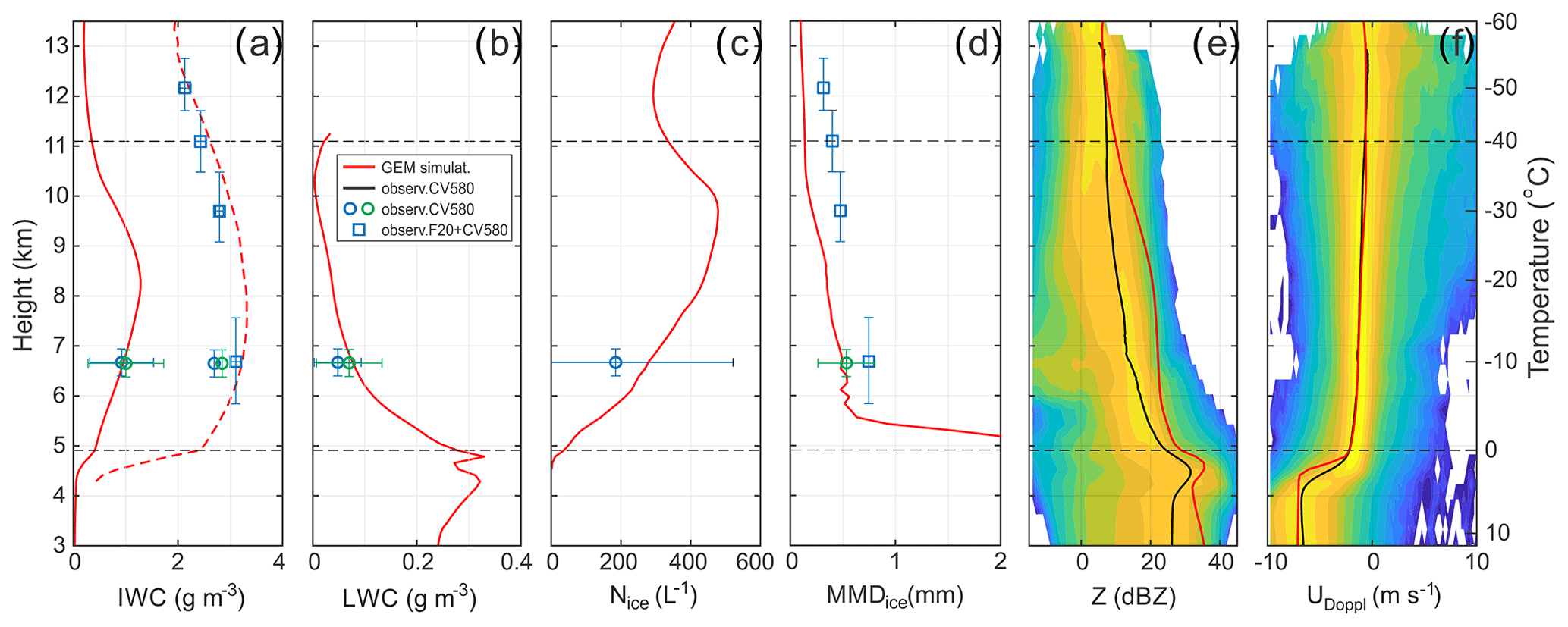
Figure 10 Comparisons of the average microphysical parameters from the GEM simulation and in situ measurements collected from CV580 (circles) and F20 (squares). (a) Simulated IWC_m (solid red) and IWC₉₉ (dashed red) measured by IKP (blue circles ) and 2D probes (green circle). (b) Mean modeled LWC (red), measured by FSSP (green circle) and CDP (blue circle). (c) Mean modeled (red) and measured (blue circle) concentration of ice N_ice with D> 40 µm. (d) Modeled D_3  ice corrected on the ice density, CV580 D_3  ice (blue circles), and measured F20 MMD_ice (blue squares). (e) Measured by the CV580 X-band radar probability density field and mean reflectivity Z (black) and modeled mean Z (red). (f) Measured by the CV580 X-band radar probability density field and mean Doppler velocity U_Doppl (black) and modeled mean U_Doppl (red). The F20 vertical error bars indicate the temperature range of the sampled data. The CV580 vertical and horizontal error bars indicate the standard deviation of the sampling statistics. Horizontal dashed lines show levels corresponding to T=0 °C (H=4.9 km) and $T=-\mathrm{40}$ °C (H=11.1 km) levels.

Figure 10a shows comparisons of the observed and modeled IWC_m and IWC₉₉. The CV580 IWC were measured by the IKP and calculated from composite PSDs measured by 2D-S and PIP. The F20 IWC was measured by the IKP (Strapp et al., 2020, 2021). The difference between measured and simulated IWC_m and IWC₉₉ does not exceed 6 % and 20 %, respectively.

Figure 10b shows comparisons of the simulated LWC_m to that calculated from the FSSP and CDP measurements. The difference between the modeled LWC_m and that measured by the FSSP and CDP is 38 % and 9 %, respectively.

For the purposes of comparison, the model N_ice was modified to match the size range of ice particles measured by the 2D-S. Since the first three size bins in 2D-S measurements were omitted due to the uncertainty in the depth-of-field definition and large errors in sizing of small particles, the 2D-S-measured N_ice did not include ice particles smaller than 40 µm. In order to make direct comparisons of observed and modeled N_ice, the ice particle sizes smaller than 40 µm were also excluded from the modeled N_ice by recomputing the concentration from the model ice PSDs but with an incomplete gamma function, starting at 40 µm. Figure 10c shows a reasonable agreement between of the corrected modeled and measured N_ice, and the deviation between the modeled and observed N_ice is 35 %.

As mentioned in Sect. 3.1.3, the modeled D_3  ice is the diameter of an equivalent mass sphere. However, the measured ice particle sizes represent one dimension of randomly oriented projections of non-spherical particles. In order to make direct comparisons between the modeled and measured ice particle sizes, the simulated D_3  ice was modified from that for unrimed ice in the original P3 microphysics scheme to D_3  corr = $(\frac{\mathit{\pi }{\mathit{\rho }}_{\text{ice}}}{a}{D}_{\mathrm{3}\text{ice}}^{\mathrm{3}}{)}^{\frac{\mathrm{1}}{b}}$, where a and b are parameters in the mass–size relation, V(D) = aD^b (e.g., Brown and Francis, 1995). The comparisons of values measured from the CV580 and the corrected simulated D_3  ice are shown in Fig. 10d.

Figure 10d also shows the median mass size MMD_ice measured from F20. MMD_ice and D_3  ice may be quite different, depending on the shape of a PSD, which makes the comparisons of these two sizes not strictly valid. As seen from Fig. 10d, the modeled D_3  ice and measured MMD_ice differ from each other by 2 to 4 times above 9 km. However, despite these differences in the definitions of the modeled and measured sizes, the observed MMD_ice profiles show a general trend in the size reduction towards the cloud top, which is similar to the behavior of the simulated D_3  ice profile.

Comparisons in Fig. 10e show that the modeled mean Z is systematically larger than the measured values, with differences reaching 10 dBZ. This is an overly large difference. The analysis of the model setup suggests that the complete gamma function for the ice PSDs in the microphysics scheme overestimates the number of large particle sizes for which higher moments such as radar reflectivity are sensitive. At the time of writing, a solution for this diagnostic problem is being examined, and the problem will be corrected in a future version of the P3 scheme. Note that small errors in the tail of the PSDs can create relatively large errors in higher moments of the PSDs (including Z) but only small errors in lower moments, such as those associated with the fields of interest (e.g., N_ice, MMD_ice, and IWC), which appears to be the case in the simulations presented. Also note that the model reflectivity field is computed as a simple diagnostic and not an instrument simulator per se; it is calculated based on Rayleigh scattering assumptions and does not account for Mie scattering for large particles for the case of X-band radar.

Despite the significant difference in reflectivity, the modeled and observed Doppler velocity values have a surprisingly good agreement. One of the explanations for such a good agreement is the weak dependence of particle fall velocity on particle size for diffusion grown ice particles (Pruppacher and Klett, 1997). In this case, the presence of artificially large particles may not have a significant effect on the Doppler velocity.

Another set of comparisons is shown in Fig. 11. Figure 11a shows modeled and observed ice number concentration versus IWC. The latter was shown earlier in Fig. 4a. For comparison purposes, the particles < 40 µm were excluded from N_ice to be consistent with the measured values. As seen in Fig. 11, the median observed and modeled ice concentrations reasonably agree to approximately 2 g m⁻³. The model produces a higher ice number concentration for IWC > 2 g m⁻³ than those observed in situ.

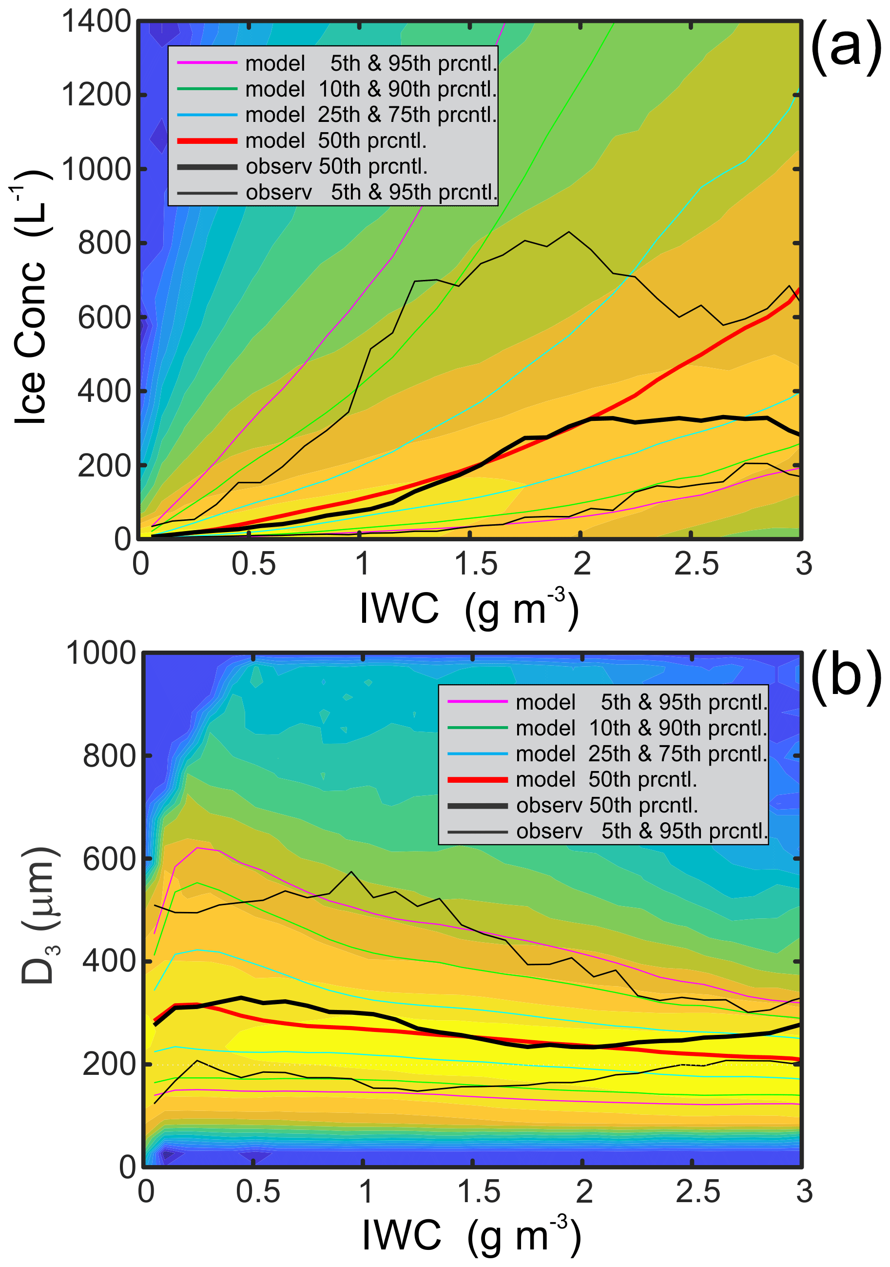
Figure 11 Comparisons of modeling results and in situ observations of IWC, D_3  ice, and N_ice. Fields of modeled (a) concentration of ice particles > 40 µm vs. IWC and (b) equivalent volume diameter of ice particles vs. IWC. Observed median (thick) and 5th and 95th percentile (thin) values are shown in black. The modeling data were averaged over a time period from 75 to 135 min and a range of altitudes between 5.8 and 7.4 km, corresponding to the CV580 sampling altitudes.

Figure 11b shows comparisons of the modeled mean volume diameter of ice particles with those obtained from observations. In order to match the definition of the modeled ice size, the measured mean volume diameter was calculated as D_3  ice = $(\frac{\mathrm{6}}{\mathit{\pi }{\mathit{\rho }}_{\text{ice}}}\frac{\mathrm{IWC}}{N_{\text{ice}}}{)}^{\mathrm{1}/\mathrm{3}}$. As already seen, the measured and modeled median D_3  ice agree within 25 %. However, the modeled sizes have large scatter compared to the measured ones.

We emphasize that there are many limitations in this study, and these clearly illustrate the need for further laboratory, numerical, and field studies. On the measurement side, there are challenges with in situ observations such as limited sampling statistics, limitations of flight operations, and instrumentation uncertainties and errors. For the numerical model, there are challenges and limitations that include unresolved turbulent air motion, hydrometeor size distribution assumptions in the bulk microphysics scheme, incomplete knowledge of natural cloud microphysics to constrain the parameterization of individual processes, and the use of a quasi-idealized model setup. Overall, however, the GEM model simulations using the P3 microphysics scheme yield a reasonably good agreement with the in situ observations, with the caveat that observations themselves were used to derive the FFD parameterization. This provides a strong motivation to establish better FFD formulations as a potential leading mechanism of formation of HIWC environment in tropical MCSs.

3.2.2 SIP initiation

The results of the SIP-ON simulation show that the cloud environment above the melting layer is densely populated with small ice crystals (Figs. 8a, c and 9c, d). Thus, within 1 km above the melting layer, the average N_ice in the SIP-ON run exceeds that of BASE by 2 orders of magnitude (Fig. 9c). Since the inclusion of the FFD and HM processes in the SIP-ON simulation is the only difference between the SIP-ON and BASE configurations, the enhanced concentration of ice particles above the melting layer in the SIP-ON simulation is unambiguously attributed to the secondary ice processes.

Of the two additional processes included in the SIP-ON simulation, the Hallett–Mossop (HM) process was found to be significantly less efficient in producing secondary ice compared to FFD (Fig. 8g). Therefore, the main contribution to the ice concentration is from the FFD. Equation (1) shows a strong dependence on the drop size, which suggests that the FFD rate will be most efficient in presence of large drops. This raises the question of the source of large drops inside deep-glaciated MCSs.

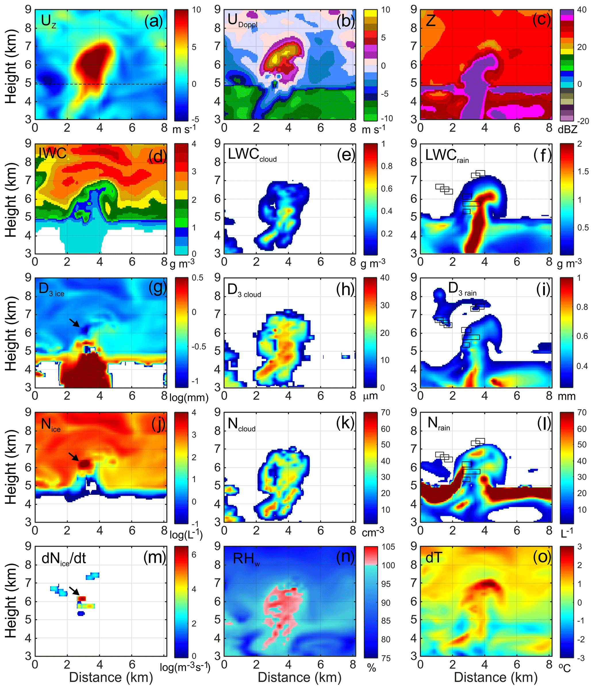
Figure 12 Model microphysical and thermodynamical fields illustrating the effects of recirculating raindrops in convective updrafts on the FFD process. (a) Vertical velocity U_z; (b) Doppler velocity U_Doppl; (c) radar reflectivity Z; (d) IWC; (e) LWC_cloud; (f) LWC_rain; (g) mean mass diameter of ice D_3  ice; (h) mean mass diameter of cloud droplets D_3  cloud; (i) mean mass diameter of raindrops D_3  rain; (j) ice particle number concentration N_ice; (k) cloud droplet number concentration N_cloud; (l) raindrop number concentration N_rain; (m) SIP rate $\mathrm{d}{N}_{\text{ice}}/\mathrm{d}t$; (n) relative humidity over liquid RH_w; (o) temperature perturbation ΔT. The rectangles in (f), (i), (l) indicate locations of the active SIP regions shown in (m).

The set of diagrams in Fig. 12 presents vertical 6 × 8 km fields of the main microphysical fields of interest intersecting a convective updraft in the vicinity of the melting layer. As seen from Fig. 12a, the vertical updraft starts at approximately 3 km and extends above 7 km. The convective updraft results in supersaturation over water (Fig. 12n) and the activation of cloud droplets (Fig. 12e, h, and k). The boundary of the water supersaturation region (Fig. 12n) and newly formed cloud (Fig. 12e, h, and k) follows the pattern of the convective plume (Fig. 12a).

The Doppler velocity field in Fig. 12b shows that the majority of cloud particles above the melting layer are moved upward within this convective updraft. The depression of 5 m s⁻¹ of the Doppler velocity field with respect to the neighboring region below the melting layer indicates that precipitation size drops with D > 2 mm are lifted by the updraft. Smaller-sized drops will have higher upward velocity in the updraft, and they will be brought up by the updraft to higher altitudes during the same time period. This is consistent with the D_3  rain field (Fig. 12i), which shows that 1 mm drops did not ascend through the melting layer because of the slow vertical velocity of their ascent. However, drops with D < 500 µm have a small enough fall velocity to be moved by the convective updraft above the melting layer.

Figure 12l shows how a convective updraft affects the field of the concentration of raindrops N_rain. It is worth noting that the top of the melting layer is densely populated with a large number of small-sized rain and drizzle drops, the concentration of which may reach several hundred per liter. The small sizes of these small drops are explained by the melting of small secondary ice particles, which melt rapidly below the freezing level. The concentration of raindrops in the melting layer of BASE is lower because of the lower ice concentration, and the size of the raindrops is larger because of larger ice particles compared to the SIP-ON simulation.

The upward transport of rainwater through the melting layer (Fig. 12a and f) eventually manifests in the disturbance of the bright band (Fig. 12c). Similar disturbances of the bright band are observed in situ (Figs. 6a and 7a). Note that the patterns of the fields of LWC_rain, N_rain, and D_3  rain do not coincide with that of LWC_cloud, N_cloud, and D_3  cloud; this suggests that the rainwater is primarily transported by the updraft from underneath of the melting layer rather than being formed locally though the collision–coalescence process of cloud water. However, accretion of cloud water may contribute to the enhancement of raindrop sizes.

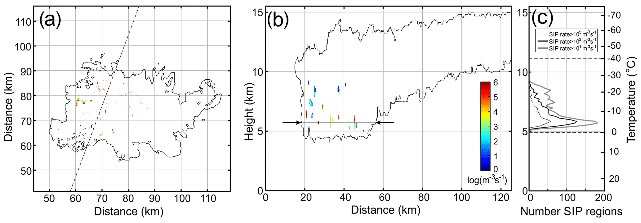
Figure 13 Cloud regions with active SIP simulated at 90 min. (a) Horizontal cross section of the SIP rate field at H = 5.8 km and T = −5 °C. (b) Vertical section of SIP rate field along the line indicated by the dashed line in panel (a). Arrows in panel (b) indicate the level of the horizontal section shown in panel (a). Thin black lines (a, b) indicate cloud boundaries at the isoline of ice concentration at the threshold N_ice = 0.01 L⁻¹. (c) Vertical profiles of the number of spatially isolated SIP regions at different SIP rate thresholds for the cloud shown in panels (a) and (b).

The high value of $\mathrm{d}{N}_{\text{ice}}/\mathrm{d}t$ results in the increase in N_ice (Fig. 12j; location indicated by the arrow). As expected, the newly formed particles in the region with enhanced concentration have smaller sizes (Fig. 12g; indicated by arrow) due to their smaller age.

Figure 12m shows that the field of the high SIP rate $\mathrm{d}{N}_{\text{ice}}/\mathrm{d}t$ (peak location indicated by the arrow) occurs inside the fields of LWC_rain, N_rain, and D_3  rain in Fig. 12f, i, and l, but it does not necessarily coincide with their peak values. The area maximum values of $\mathrm{d}{N}_{\text{ice}}/\mathrm{d}t$, indicated by rectangles in Fig. 12f, i, and l, are offset from the local maxima of LWC_rain, N_rain, and D_3  rain. One of the reasons for that is that besides the droplet size, the FFD rate also depends on temperature, the concentration of large drops, the ice particles sizes, and their concentrations. Consequently, combinations of these five fields may result in local maxima of $\mathrm{d}{N}_{\text{ice}}/\mathrm{d}t$, which are not necessarily coincident with the individual maxima of N_rain, D_3  rain, N_ice, and D_3  ice.

Freezing of cloud and raindrops and the depositional growth of numerous secondary ice particles result in the release of latent heat, which will subsequently lead to positive temperature perturbations. The local temperature perturbation near the top of the updraft reaches approximately 3 °C (Fig. 12o). Such high-temperature fluctuations will result in the invigoration of convection above the melting layer.

The analysis of the numerous cases similar to that in Fig. 12 across the model domain suggests that convective updrafts play a key role in transporting precipitation size drops across the melting layer. The presence of large drops provides one of the necessary conditions for initiating the FFD process. However, just the presence of the large drops is not sufficient for triggering the FFD chain reaction; there are four other criteria required for efficient SIP production, i.e., (1) drop concentration, (2) size of ice particles, (3) concentration of ice particles, and (4) temperature, must be also met. The optimum conditions for the FFD $\mathrm{d}{N}_{\text{ice}}/\mathrm{d}t$ may not necessarily occur inside the updrafts intersecting the melting layer, but rather they may happen somewhere in their vicinity of the convection when the outflow of large drops mixes with the pre-existing ice outside of the convective plume.

3.2.3 Spatial and temporal characteristics of SIP regions

One of the important aspects of HIWC formation is understanding where, when, and at what rate ice initiation occurs. This section analyzes the rates of ice production and spatial distributions of SIP regions in the model domain. Given that the FFD SIP process is the main contributor to ice production, for the sake of conciseness, the following analysis is focused on the FFD regions, and the discussion of the role of the HM is omitted.

Figure 13a and b show horizontal and vertical cross sections of the FFD rate fields inside the modeled MCSs. The horizontal cross section in Fig. 13a refers to the altitude of 5.8 km (−5 °C), as indicated by two arrows in Fig. 13b, and the vertical section in Fig. 13b was done along the dashed line in Fig. 13a. As seen from these diagrams, $\mathrm{d}{N}_{\text{ice}}/\mathrm{d}t$ varies within several orders of magnitude and may reach 10⁷ ${\mathrm{m}}^{-\mathrm{3}}{\mathrm{s}}^{-\mathrm{1}}$.

Figure 13a and b show that regions of secondary ice production have highly clustered spatial structures. The vertical changes in the number of the isolated SIP regions (n_SIP) integrated over each model level in Fig. 13a and b are shown in Fig. 13c. As seen from Fig. 13c, n_SIP depends on the threshold of $\mathrm{d}{N}_{\text{ice}}/\mathrm{d}t$. The general trend of the vertical changes in n_SIP for all three SIP thresholds remains the same, and they all reach a maximum at the same altitude ∼ 5.8 km (−5 °C). The production of secondary ice extends up to 9.2 km, which corresponds to −25 °C, the lowest temperature of the FFD process (Keinert et al., 2020).

Figure 14 shows the frequency distributions of the horizontal F(L_h) and vertical F(L_v) lengths of the SIP regions. These distributions were integrated over the cloud layer between 5.2 and 9.2 km (30 model levels). The mean values of L_h and L_v are equal to 340 and 190 m, respectively. However, in terms of the modeled grid cell dimensions (i.e., horizontal = 250 m and vertical ≈ 145 m) the mean values of L_h and L_v are 1.36 and 1.31, respectively. That is, in the modeled space, the shapes of SIP regions are isometric, with L_h ≈ L_v. This suggests that the resolution of the model may not be sufficient to resolve the actual dimensions of the SIP regions and that SIP is an essentially a subgrid process (within the context of a model with a 250 m horizontal grid spacing).

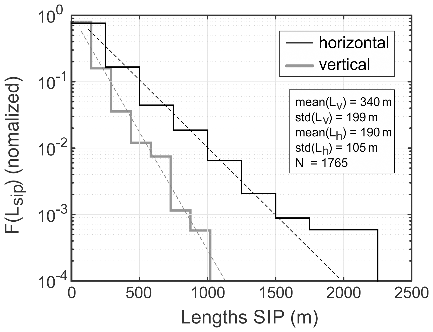
Figure 14 Frequency distributions of vertical L_v and horizontal L_h lengths of SIP cloud regions with the SIP rate > 10³ ${\mathrm{m}}^{-\mathrm{3}}{\mathrm{s}}^{-\mathrm{1}}$. The spatial averaging was performed over the in-cloud layer 5.0 < H < 9.2 km at 90 min of modeled cloud. Dashed lines are the parameterization of the frequency distributions.

Both F(L_h) and F(L_v) can be well parameterized by an exponential function $F\left(L\right)=a{e}^{-bL}$, where a_v = −8.2 × 10⁻³, b_v = 0.024, a_h = −4.7 × 10⁻³, and b_h = 0.089. As follows from Fig. 14, approximately 75 % of active SIP regions L_h and L_v have scales of approximately one grid cell, i.e., 250 and 145 m, respectively.

The F(L_h) and F(L_v) distributions were calculated for the SIP regions with the rate $\mathrm{d}{N}_{\text{ice}}/\mathrm{d}t$ > 10³ ${\mathrm{m}}^{-\mathrm{3}}{\mathrm{s}}^{-\mathrm{1}}$. Calculations of F(L_h) and F(L_v) for other SIP thresholds in the range 10¹ ${\mathrm{m}}^{-\mathrm{3}}{\mathrm{s}}^{-\mathrm{1}}$ < $\mathrm{d}{N}_{\text{ice}}/\mathrm{d}t$ < 10⁵ ${\mathrm{m}}^{-\mathrm{3}}{\mathrm{s}}^{-\mathrm{1}}$ showed that it does not have any significant effect on the shape of the distributions in Fig. 14, and the mean values of L_h and L_v vary within only 7 %.

Another important characteristic of SIP regions is their spatial occurrence. Figure 15 shows the vertical profiles of the area fraction and the average distance between SIP regions. The area fraction is defined as the ratio of the area of all SIP regions in the modeled layer to the area of the horizontal cloud cross section at that level. The cloud cross-sectional area was calculated for the environment with N_ice > 0.01 L⁻¹ (e.g., Fig. 13a). As seen in Fig. 15a, the SIP area fraction varies between 0.2 % and 2 %, depending on the SIP rate threshold, and its maximum occurs between 5.5 and 5.8 km. This altitude corresponds to the maximum rate of SIP (Fig. 8g) and maximum number of SIP regions (Fig. 13c). The average distance between SIP regions (Fig. 15b), depending on the SIP threshold, varies from approximately 30 to 100 km at the level of maximum SIP occurrence (5.5 to 5.8 km). Above and below this altitude, the average distance between SIP regions rapidly increases.

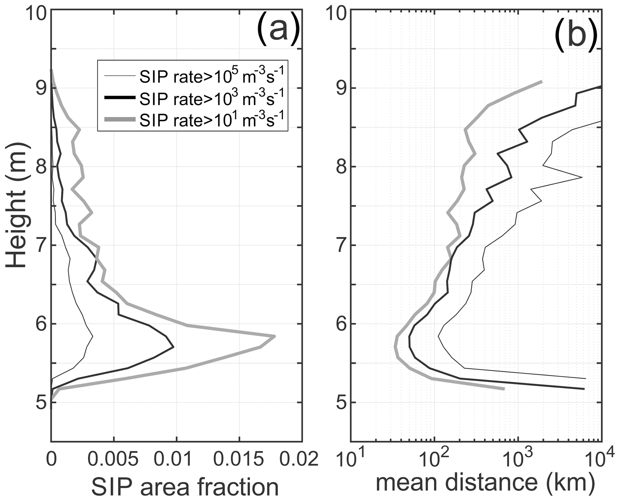
Figure 15 Vertical profiles of (a) the area fraction and (b) mean distance between the SIP cloud regions.

Endurance of the individual SIP regions is an important parameter affecting the formation and maintenance of the HIWC environment. The lifetime of individual SIP cloud regions can be estimated from the animations of the modeled cloud regions with the SIP rate $\mathrm{d}{N}_{\text{ice}}/\mathrm{d}t$ > 10⁵ ${\mathrm{m}}^{-\mathrm{3}}{\mathrm{s}}^{-\mathrm{1}}$ available in the Supplement (Korolev et al., 2024). Visual analysis of the animations allowed a rough assessment showing that the endurance of the SIP regions is of the order of 10¹–10² s⁻¹, with an average of close to 2–3 min. Typically, small SIP regions with a horizontal extent of a few hundred meters have a relatively short lifetime of 20 to 40 s. Meanwhile, the lifetime of SIP regions over a few kilometers may reach over 10 min. The lifetime of the FFD SIP regions is primarily determined by the presence of large drops, which are depleted with time due to freezing on impact with secondary or preexisting ice particles, precipitating out of the cloud volume, and through evaporation due to the WBF process.

The primary findings of this section can be summarized as follows. The FFD SIP regions are short-lived cloud objects (∼ 10² s) with spatial scales of the order of hundreds of meters. The area fraction of SIP regions is quite small and typically less than 1 %. At the level of their maximum SIP occurrence, the average distance between the SIP regions is of the order of tens of kilometers. Altogether, the spatial sparsity and short lifetime make the SIP regions challenging objects for in situ observations.

Existing observational techniques do not allow for measurements of SIP rates. However, the spatial scales of the cloud regions that experienced SIP in the recent past could be estimated from the measurements of horizontal lengths of cloud regions with enhanced concentrations of small facetted ice crystals (D_max < 100 µm). Such small ice crystals, due to their young age, are still associated with the location of their origin, and the dimensions of the cloud regions affected by SIP have not yet been significantly changed by turbulent diffusion. Therefore, the dimensions of the cloud regions with enhanced concentrations of small ice particles can be used as a proxy for the active SIP regions. Thus, Korolev et al. (2020; Figs. 5a and 23a) showed that the typical horizontal dimensions of such cloud regions are of the order of a few hundred meters. The same study showed that SIP regions are separated by tens of kilometers. Therefore, spatial scales, the clustering of SIP cloud regions, and the distance between them obtained in simulations are generally consistent with the in situ observations.

4 Summary of observations and modeling

Prior to the formulation of the conceptual model of HIWC, we summarize the main outcomes of in situ observations (Sect. 2) and numerical simulation (Sect. 3), which are relevant to the understanding of the formation of HIWC:

1. Small facetted hexagonal prisms (D_max < 100 µm) with measured number concentrations N_ice up to ∼ 10³ L⁻¹ were observed above the melting layer at temperatures of T < −2 °C. The enhanced concentrations of small ice particles were attributed to the massive production of secondary ice (Sect. 2.3).

2. The secondary ice production cloud regions with enhanced concentrations of small facetted ice were frequently accompanied by observations of supercooled large drops (D < 300 µm), deformed frozen drops, and fragments of frozen drops. This enables the hypothesis that the main mechanism of SIP is the fragmentation of freezing drops (FFDs) (Sect. 2.3).

3. Cloud regions experiencing SIP were sparse and had small horizontal extents (i.e., of the order of 10² m). SIP regions were typically associated with convective regions (Sect. 3.2.3).

4. The dominating ice shapes in tropical MCSs has a distinct pattern in the vertical direction above the melting layer with “small hexagonal prisms” → “columns” → “capped columns”. Such vertical changes in the ice particle habits can be explained by metamorphosis of ice particles when they experience successive columnar growth (−9 °C < T < −2 °C) followed by plate growth (−22 °C < T < −9 °C) regimes. The observed changes in ice particles in the vertical direction suggest that the small ice particles formed in the vicinity of the melting layer were transported upwards by the convective updrafts and went through columnar and then plate growth regimes (Sect. 2.4).

5. The HIWC cloud regions on average have significantly higher concentrations and smaller ice particles compared to the cloud regions with low IWC (Sect. 2.3; Figs. 3 and 4; Table 1).

6. Mixed-phase cloud regions in mature MCSs are sparse and occupy only a few percent of in-cloud space at −5 °C. Mixed-phase cloud regions were primarily observed in convective updrafts, which can force the coexistence of the ice and liquid phase (Sect. 2.5).

7. Spatially sparse large drops (100 µm < D < 300 µm) with number concentration < 10⁻³ L⁻¹ were observed at 1–2 km above the melting layer in the vicinity of updrafts. In the absence of any significant LWC layers, the only source of these large drops could be the precipitating size drops formed below the melting layer and then transported upward by convective updrafts (Sect. 2.6).

8. The disturbance of the bright band was typically observed in convective regions and is explained by vertical transport of melting ice, along with precipitation size drops, through the melting layer in an upward direction (Sect. 2.7).

9. HIWC cells are associated with convective updrafts existing somewhere inside these cells (Sect. 2.8).

The numerical model simulation (SIP-ON configuration) reproduced the observed large concentration of ice particles above the melting layer, with an average ranging from 10² to 10³ L⁻¹ and peaking up to 10⁴ L⁻¹. The main mechanism of ice initiation was related to the FFD process.

The model was able to reproduce the high clustering and sparsity of SIP regions when using a parameterization that was based on previous aircraft measurements. The typical horizontal dimensions (10²–10³ m) and distances between SIP regions (10¹–10² km) are generally consistent with observations. The model qualitatively and quantitatively reproduced trends of vertical profiles of IWC, LWC, N_ice, D_3  ice, Z, and U_Doppl (Fig. 10) and the general relations between N_ice and D_3  ice versus IWC (Fig. 11).

The numerical modeling confirmed the hypothesis of transport of precipitation size drops through the melting layer by convective updrafts (Korolev et al., 2020). The model also reproduced the disturbance of the bright band and justified the hypothesis of disturbance of the bright band by convective updrafts. The vertical transport of precipitation size drops creates an environment above the melting layer favorable for the SIP FFD process.

The agreement between in situ observations and numerical simulations creates a basis for the following conceptual model of the formation of HIWC cloud regions in tropical MCSs.

Figure 16 Illustration of a conceptual model of HIWC formation in tropical MCSs.

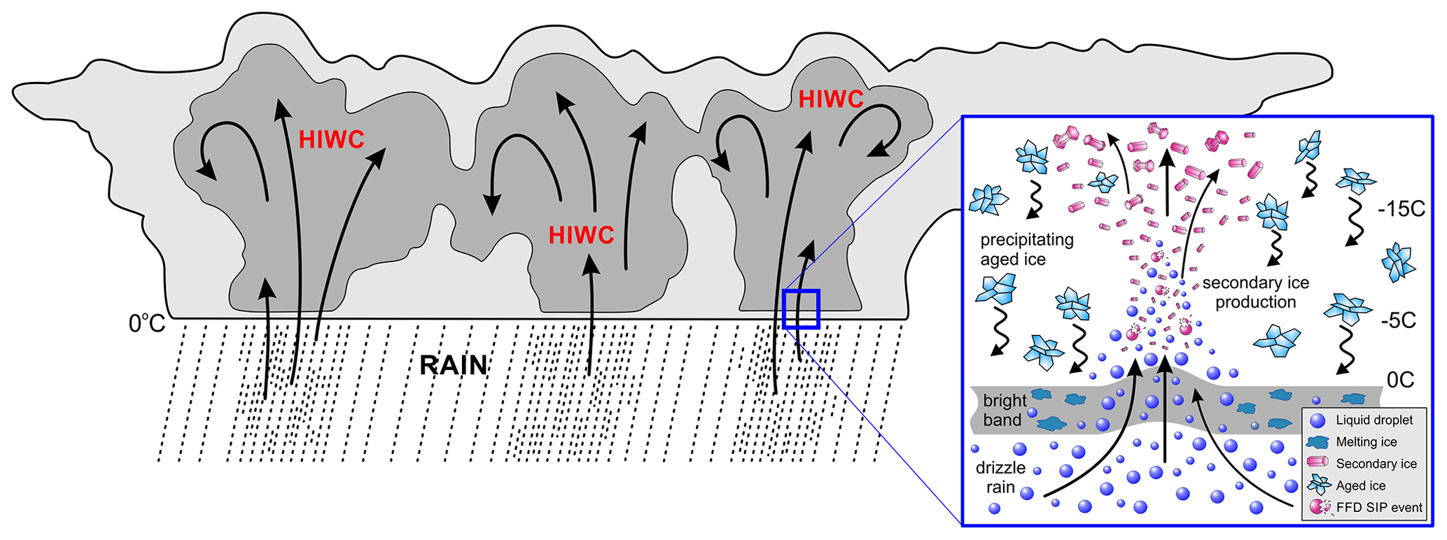
Conceptual model of HIWC

The combination of in situ observations and numerical simulations enables us to make the following general conclusions regarding the formation of HIWC in oceanic tropical MCSs. The process begins with forming a melting layer in a convective environment during the early stage of MCSs. Updrafts generated by regular convection or gravity waves transport precipitation sized drops from below the melting layer to above it. Above the melting layer, large supercooled drops create a favorable environment for the FFD SIP process. FFD yields a massive production of secondary ice particles within 1 to 1.5 km above the melting layer, with a maximum of around −5 to −8 °C. Freezing drops and rapid depositional growth of large amounts of ice particles result in the enhanced release of the latent heat and invigoration of the convection. During the subsequent updraft, the ensemble of small ice crystals rapidly depletes the supersaturated water vapor, increasing IWC, and thereby forming the HIWC environment. High concentrations of secondary ice particles lead to intense competition for the water vapor, which hinders their growth. As a result, ice particles constituting the HIWC environment remain small in size. The convective updrafts transport small ice particles to higher altitudes and distribute them throughout the stratiform regions.

Convective updrafts across the MSC domain periodically pump small ice crystals to high altitudes, maintaining the HIWC environment there. The maintenance of HIWC is also facilitated by small sizes of ice particles, which may remain suspended in the cloud for a longer time due to the small fall speeds. Overall, HIWC environments are dynamic cloud objects that form due to a balance between particle sedimentation and IWC brought up by convection.

The conceptual model of the HIWC formation is illustrated in Fig. 16.

While the proposed conceptual model is based on a relatively limited number of in situ observations (focused on one specific geographical location) and quasi-idealized numerical model simulations, both of which have limitations and challenges, the central point of the conceptual model is that HIWC environments in tropical MCSs form as a result of the intensive production of secondary ice particles at temperatures just below freezing (primarily −10 °C < T < −2 °C), which are then transported to high altitudes (∼ 7 < H < 15 km) by convective updrafts. This part of the conceptual model is well justified, based on in situ observations, and can be considered an established experimental fact.

However, despite observational evidence indicating that the FFD process is the major contributor to the production of secondary ice, this part of the conceptual model requires more in situ observations and especially laboratory studies. The latter is crucial for detailed studies on the dependence of FFD rates in environmental conditions and the development of physically based parameterizations that can be used in numerical simulations. The simulations examined in this study support the hypothesis that FFD SIP alone is sufficient to explain the large amounts of ice generated without involving other SIP mechanisms (Korolev and Leisner, 2020; James et al., 2021). That said, the authors acknowledge that the FFD mechanism is not well established in the laboratory, and the contribution of other mechanisms also remains uncertain and requires further study.

5 Concluding remarks

The mechanism of HIWC formation described above is specifically relevant to tropical oceanic MCSs, which are characterized by a low aerosol load and relatively moderate convection with vertical velocities peaking at 15 to 20 m s⁻¹. We emphasize that the roles and contributions of different cloud processes in HIWC depend on the initial environmental parameters, and it may be different for continental and midlatitude convective systems compared to HIWC in maritime tropical MCSs. Results of the baseline simulation, with SIP processes off, suggest that any convective system, if strong enough, may generate a HIWC environment. However, the bulk properties of the population of ice particles comprising HIWC, such as MMD, reflectivity, and IWC, may be different from those observed in the tropics. For example, as discussed in Lawson et al. (2015, 2023), the high aerosol load in continental convective systems may suppress SIP. One of the consequences of SIP suppression is the high production of graupel/hail, increased radar reflectivity, and a relatively low ice number concentration. This case would be equivalent to the HIWC environment in the BASE simulations, as described in Sect. 3.2 (Fig. 8). Due to the larger particle sizes and, therefore, higher fall velocity, the endurance of the HIWC environment in such clouds will be shorter compared to those in tropical MCSs with smaller ice particles.

We reiterate that while the numerical simulations presented in this study support the proposed conceptual model for the importance of SIP in the production of HIWC in tropical convection, no claim is made regarding the fidelity of the model in accurately simulating the fundamental processes involved in SIP. Besides the model setup being quasi-idealized, the FFD parameterization itself in the microphysics scheme is ad hoc and is essentially constructed to give good results. Unfortunately, laboratory measurements remain insufficient to support the accurate model representation of FFDs conclusively. The original FFD formulation in Lawson et al. (2015) is essentially an empirical parameterization based on observations; in this study, we have adjusted it further to produce peak FFD rates at relatively warm temperatures (in contrast to laboratory studies) in order to improve the simulations. The utility of this model “tuning” approach is that while we have insufficient knowledge of the fundamental physics on which a credible FFD parameterization can be based, we can at least introduce what may be considered a compensating model error such that the end result (i.e., the numerical simulation with SIP on) is sufficiently close to the in situ microphysical observations so that we can use the simulation to further examine the model storm and to lend support to the largely observation-based conceptual model.

The significance of the initial environmental conditions for the bulk properties of the HIWC environment was supported by the recent in situ observations of the HIWC cloud regions in cold season mid-latitude frontal clouds (Rugg et al., 2022). Despite the small data set, it was found that in the mid-latitude winter clouds, MMD in HIWC regions (Fig. 10 in Rugg et al., 2022) was higher compared to those in tropical MCSs (Fig. 17 in Strapp et al., 2021). These comparisons indicate the need for more observational and modeling studies of bulk properties of HIWC cloud regions in different geographical regions with different environmental backgrounds. An especially high priority should be placed on furthering reproducible laboratory-based parameterizations of FFD and other SIP mechanisms.

Appendix A

Figure A1 Zoomed-in images of cloud particles in Fig. 1a (top) showing details of shapes of secondary ice (highlighted in blue) and frozen drops (highlighted by green frames). Numbers inside the image frames indicate the maximum size of the particle images in micrometers.

Appendix B

Figure B1 GOES-13 satellite infrared and visible images with the Convair-580 flight track for the flight segments shown in (a, b) Fig. 6 and (c, d) Fig. 7.

Appendix C

Table C1 Summary of GEM configuration details.

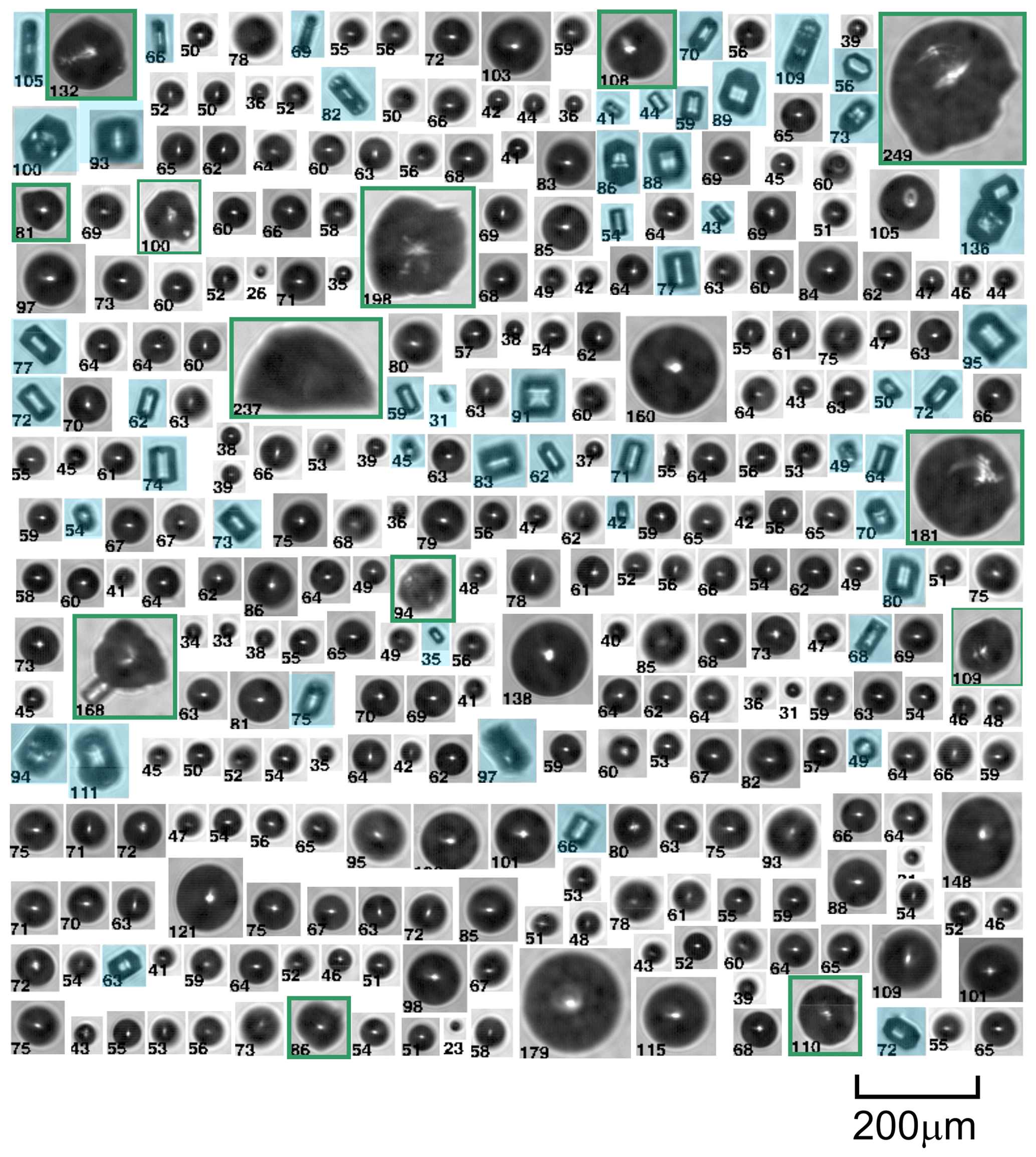
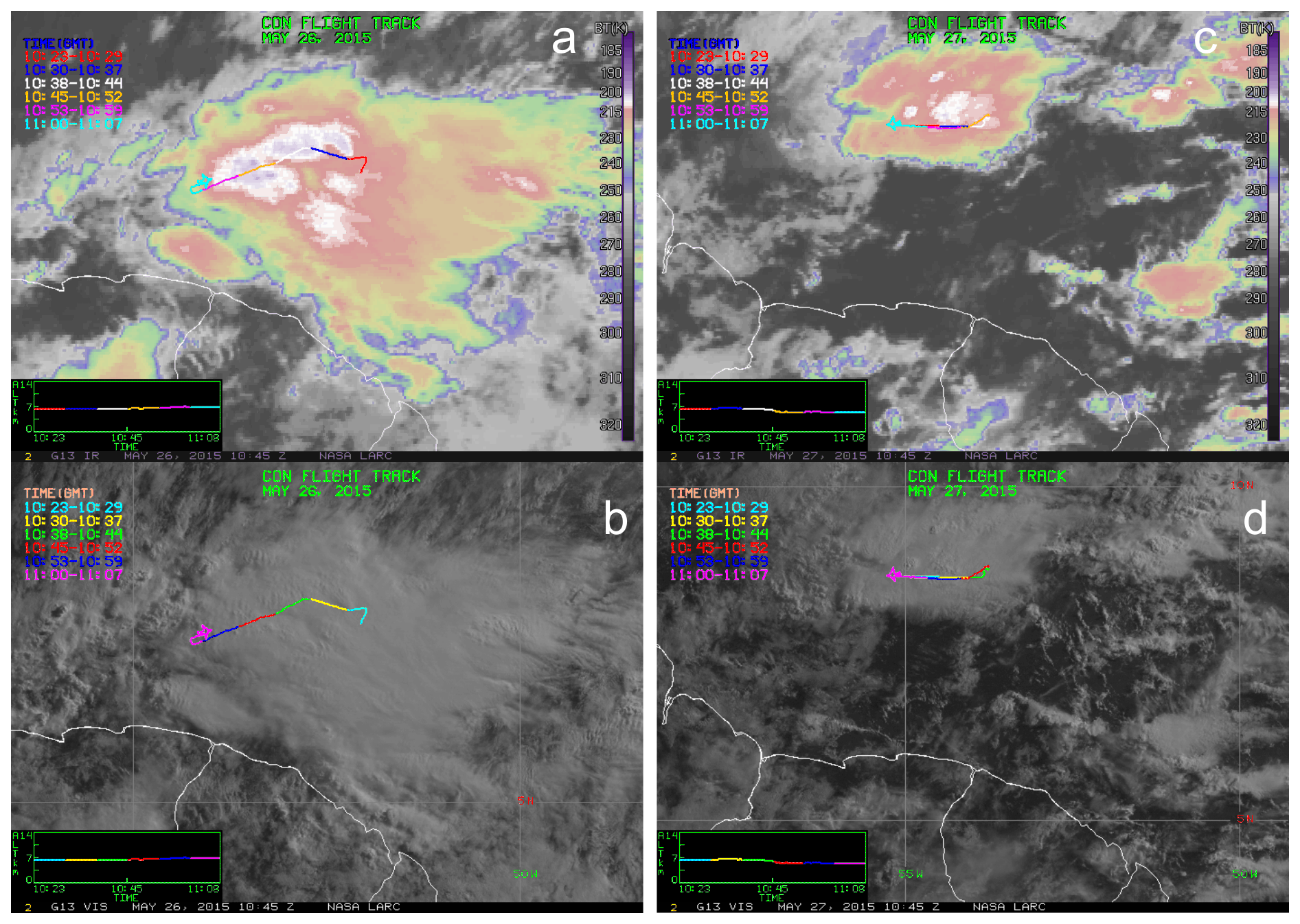
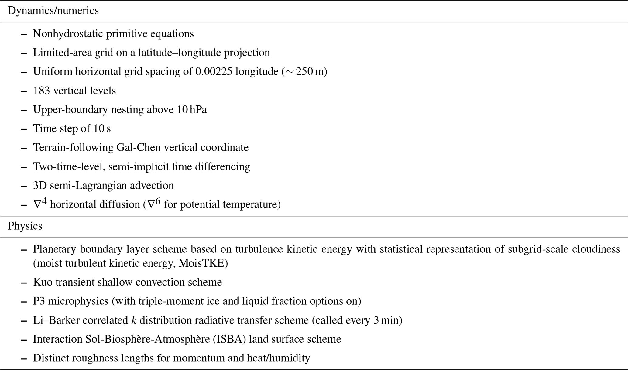
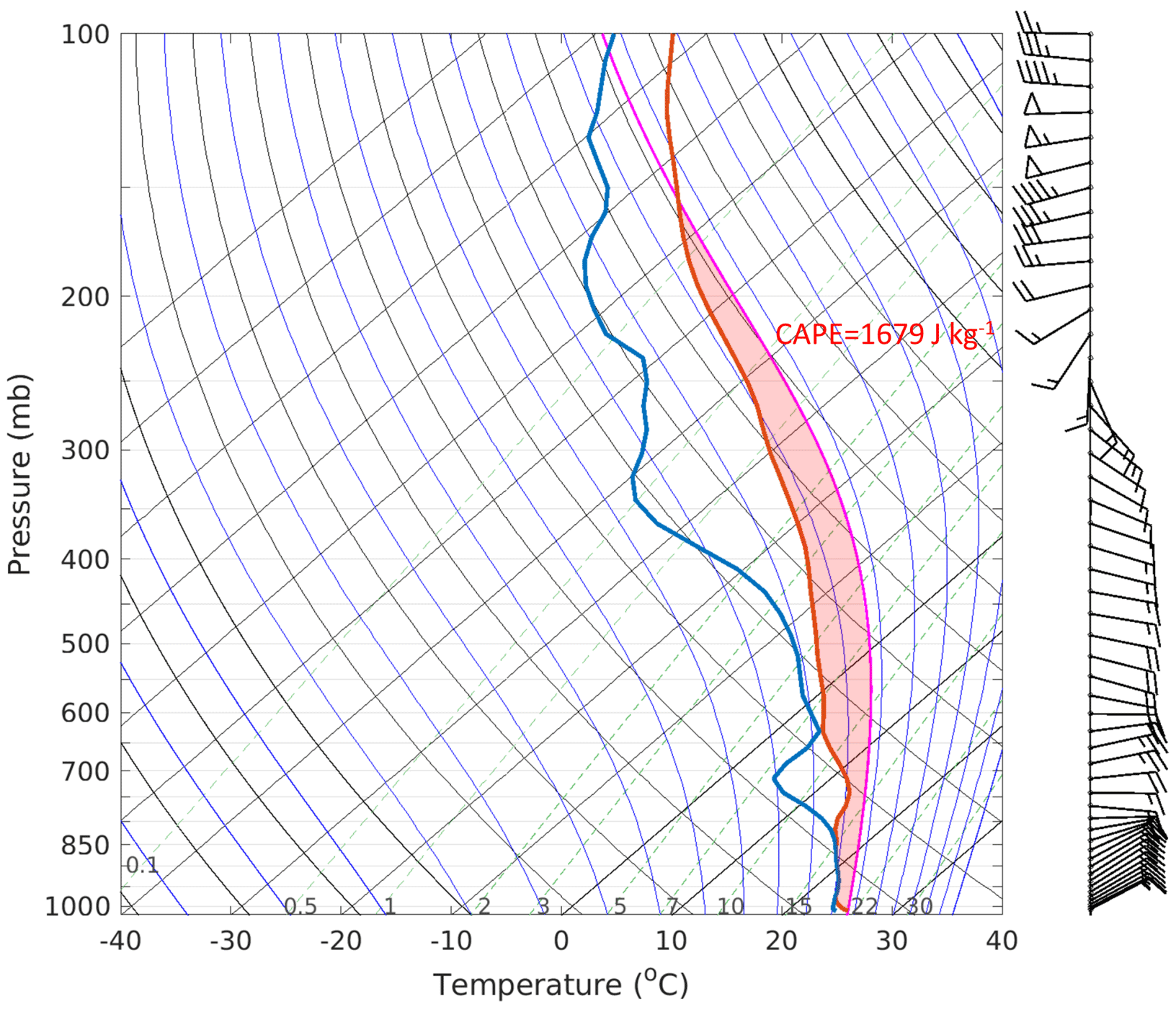
Figure C1 Initial atmospheric profiles for the idealized simulations. The blue line represents the dew point temperature, the red line represents the environment sounding (temperature), and the magenta line represents the parcel lapse rate (Qu et al., 2022).

Appendix D

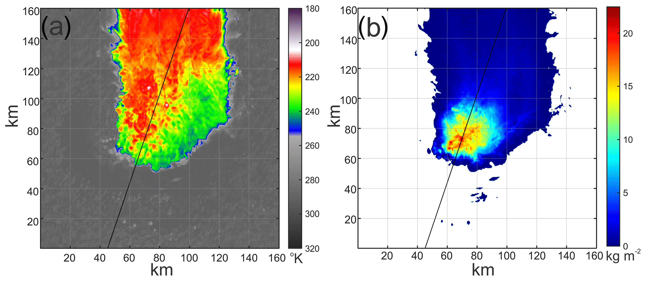
Figure D1 Brightness temperature at 11.2 µm (a) and ice water path (b) of the GEM simulated cloud system at 90 min. Black lines indicate the cross sections of the microphysical fields shown in Fig. 8.

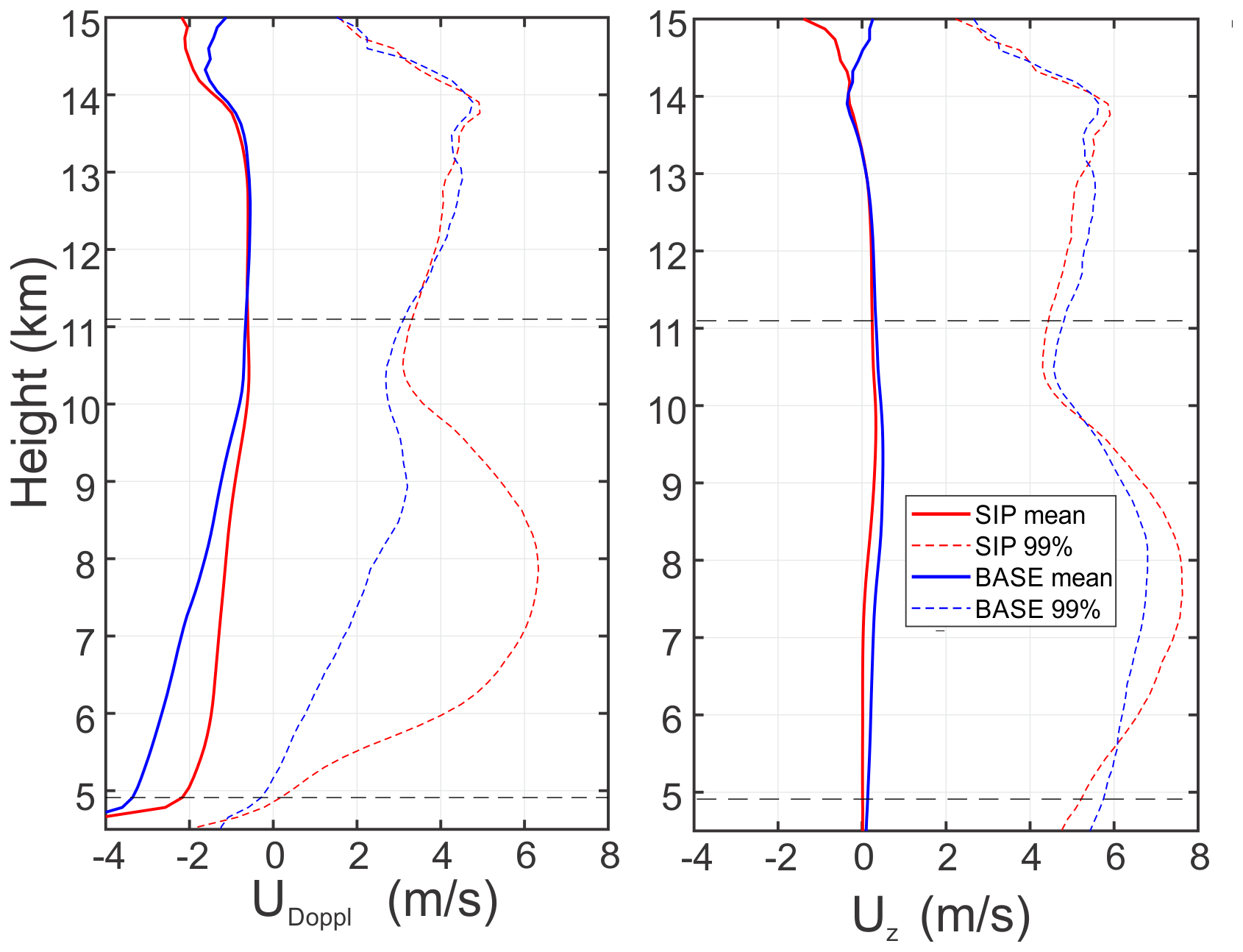
Figure D2 Average vertical profiles of GEM-simulated Doppler velocity U_Doppl and vertical wind velocity U_z. The averaging was performed over a time period from 75 to 135 min.