Multi-year gradient measurements of sea spray fluxes over the Baltic Sea and the North Atlantic Ocean

Ship-based measurements of sea spray aerosol (SSA) gradient fluxes in the size range of 0.5–47 µm in diameter were conducted between 2009–2017 in both the Baltic Sea and the North Atlantic Ocean. Measured total SSA fluxes varied between 8.9 × 10³ ± 6.8 × 10⁵ m⁻² s⁻¹ for the Baltic Sea and 1.0 × 10⁴ ± 10⁵ m⁻² s⁻¹ for the Atlantic Ocean. The analysis uncovered a significant decrease (by a factor of 2.2 in the wind speed range of 10.5–14.5 m s⁻¹) in SSA fluxes, with chlorophyll a (chl a) concentration higher than 3.5 mg m⁻³ in the Baltic Sea area. We found statistically significant correlations for both regions of interest between SSA fluxes and various environmental factors, including wind speed, wind acceleration, wave age, significant wave height, and wave Reynolds number. Our findings indicate that higher chl a concentrations are associated with reduced SSA fluxes at higher wind speeds in the Baltic Sea, while the influence of wave age showed higher aerosol emissions in the Baltic Sea for younger waves compared to the Atlantic Ocean. These insights underscore the complex interplay between biological activity and physical dynamics in regulating SSA emissions. Additionally, in both measurement regions, we observed weak correlations between SSA fluxes and air and water temperature and between SSA fluxes and atmospheric stability. Comparing the Baltic Sea and the North Atlantic, we noted distinct emission behaviors, with higher emissions in the Baltic Sea at low wave age values compared to the Atlantic Ocean. This study represents the first comparative analysis of SSA flux measurements using the same methodology in these contrasting marine environments.

1 Introduction

1.1 Sea spray properties and source processes

The sea and ocean surface is one of the two largest natural aerosol sources (Seinfeld and Pandis, 2006). The production of marine primary aerosol, often referred to as sea spray aerosol (SSA), remains a poorly understood aspect of the marine boundary layer (Quinn et al., 2017). The multitude of factors influencing SSA emission and subsequent turbulent transport contribute to significant uncertainty in global estimates of SSA production (Tsigaridis et al., 2013). This uncertainty derives from several processes that are not well understood: the turbulence in the atmospheric surface layer and the turbulence in the surface ocean and their interaction, therefore including the formation of waves; wave breaking; and entrainment processes. It also encompasses the formation of bubble clouds from the entrained air and the formation of water droplets from the bubbles. A substantial gap of knowledge is present within the aforementioned processes. However, accurate estimates of SSA flux and precise parameterization of its vertical transport through turbulent diffusion are essential across various branches of geoscience (de Leeuw et al., 2011).

The release of SSA from the sea surface is initiated by wind-induced wave breaking (Nilsson et al., 2001, 2021; Yang et al., 2019; Bruch et al., 2023; Zinke et al., 2024). Following wave breaking, air bubbles are entrained into the water column, ascend to the surface, and burst. Traditionally, two types of aerosol droplets resulting from this bubble bursting are identified, namely film and jet drops (Spiel, 1998; Woolf et al., 1987). In high-wind conditions, spume drops are also emitted from the sea surface (Mehta et al., 2019). Subsequently, turbulent diffusion intercepts all three types of droplets, transporting them into the atmosphere within the marine boundary layer.

SSA plays a crucial role in atmospheric chemistry, acting as a primary source of both inorganic and organic aerosol (Cochran et al., 2017); moreover, SSA can act as a sink for semi-volatile gases (biogenic or anthropogenic) and can prevent secondary aerosol generation, including new particle formation (Carslaw et al., 2010). SSA also affects the atmospheric load of cloud condensation nuclei (CCN) and cloud physics (Xu et al., 2022). The chemical composition of SSAs and their degree of internal mixing are other areas of research with large gaps, and these are probably closely connected to the formation of bubbles, since it is known that, while the bubble plumes rise towards the sea surface, they have a great affinity to collect all sorts of surfactants, first enriched in the bubbles and, as the bubbles burst, also enriched in the SSA. This applies to both natural organic surfactants (Facchini et al., 2008) and anthropogenic surface active substances (Oppo et al., 1999; Johansson et al., 2019).

Once acting as CCN, SSAs may interfere with water-phase chemistry in the cloud droplets. Their significance extends to the global radiative balance through both direct aerosol effects (Bates et al., 2006; Mulcachy et al., 2008; Vaishya et al., 2013; Rap et al., 2013) and indirect effects by acting as CCN (O'Dowd et al., 1999; Andrae and Rosenfeld, 2008) and, as such, must be considered in regional and global climate modeling (Partanen et al., 2014).

SSA, apart from its influence on climate, has several other significant aspects. One important aspect is its role in the transport of pollutants from the sea to the air, such as perfluoroalkyl acids (Sha et al., 2020, 2021) or microplastics (Allen et al., 2020, Ferrero et al., 2022).

Moreover, the composition of SSA varies with the seasons and biological activity (Parent et al., 2023). It has been shown to contain a significant organic component (Cavalli et al., 2004; Facchini et al., 2008), which has implications for its hygroscopicity and ice-nucleation activity (Darr et al., 2018). Furthermore, SSA has been demonstrated to be geochemically important over geologic time frames due to the presence of trace elements and metal pollution in aerosols derived from sea spray (Marx et al., 2014).

Despite recognizing the significance of incorporating SSA into the aerosol budget of the marine boundary layer, the development of parameterizations for this aerosol source remains highly challenging, and a wide array of parameterizations have been proposed, drawing from both laboratory studies (Monahan et al., 1982; Mårtensson et al., 2003; Keene et al., 2007; Tyree et al., 2007; Long et al., 2011; Salter et al., 2015) and field studies (Nilsson et al., 2001; Geever et al., 2005; Norris et al., 2008, 2012; Yang et al., 2019; Nilsson et al., 2021; Zinke et al., 2024). Here, we limit the list to such studies where SSA emission fluxes were directly observed using the eddy covariance (EC) method.

The fact that sea surface is impacted by synergies of different factors causes high uncertainty in SSA emission parameterization. For instance, there are indications that sea surface temperature (SST) can influence the sea spray flux through changes in surface tension and kinematic viscosity (i.e., Bowyer et al., 1990; Mårtensson et al., 2003; Hultin et al., 2011; Zabori et al., 2012; Forestieri et al., 2018) and through changes in the bubble spectra (Salter et al., 2014; Zinke et al., 2022). The exact processes in this link are not understood, but bubble coalescence is the most likely candidate (Ribeiro and Meiwes, 2006).

1.2 Gradient method for aerosol fluxes

The studies related to the use of vertical aerosol profiles in the boundary layer have a very long history. The first vertical aerosol profile was measured by John Aitken (Aitken, 1890; Podzimek, 1989). Since these works, a great deal of progress has been made. The understanding of the aerosol profiles in the atmospheric boundary layer has increased thanks to advances in measurement techniques, such as tower measurements and lidar remote sensing.

Recent technological developments of autonomous platforms (e.g., tethered balloons, Ferrero et al., 2014, and drones, Chiliński et al., 2018) and miniaturized, low-cost sensors have led to further progress in vertical aerosol profiling. This has led to the possibility of using the gradient method (GM) for measuring marine aerosol fluxes. In this respect, this work is the continuation of research started by Petelski (2003), in which the GM was applied for the first time, evaluating aerosol profiles measured on board a ship. We present the theory of gradient flux calculation in Appendix C.

The GM has also successfully been applied to derive SSA generation functions from the North Atlantic (Petelski and Piskozub, 2006; Andreas, 2007), the Pacific Ocean (Savelyev et al., 2014), and the Baltic Sea (Petelski et al., 2014; Markuszewski et al., 2016, 2020).

The SSA source function from North Atlantic waters using the GM was calculated by Petelski and Piskozub (2006) (and was later improved by Andreas, 2007). Later, the first-generation function of sea spray for the Baltic Sea was estimated using this method (Petelski et al., 2014).

The GM was further successfully applied to ship-based measurements in the Pacific Ocean by Savelyev et al. (2014). The derived SSA fluxes were compared with the deposition method and parameterized with surface brightness temperature.

The case studies of gradient aerosol fluxes obtained from two ship-based campaigns in the Baltic Sea cruises are presented by Markuszewski et al. (2017). The results show the influence of wave properties calculated based on wave height and peak frequency on sea spray fluxes.

Another case study was presented by Markuszewski et al. (2020), where gradient sea spray fluxes were compared with underwater sound pressure level in relation to the development of a wave state. One of the main results of that study was that it showed the impact of wind history and wave development (in two regimes: developing and developed) on hydroacoustic bubble noise (represented by the power spectrum density of noise) and SSA fluxes.

1.3 Flux parameterization

In order to present sea spray dependence on different factors, so-called sea spray generation functions (SSGFs) (or source functions) are used. The first SSGF was introduced by Monahan et al. (1982), where the laboratory experiment of whitecap simulation was used. Since then, a lot of different approaches have appeared in the literature (Lewis and Schwartz, 2004; de Leeuw et al., 2011; Grythe et al., 2014; Veron, 2015).

This approach is commonly used and is represented as a combination of aerosol size distribution and driving parameterization:

$$\begin{array}{}\text{(1)}& {\displaystyle \frac{\mathrm{d}F\left(D_{\mathrm{p}},\mathit{\alpha },\mathit{\beta },\mathrm{\dots }\right)}{\mathrm{d}{D}_{\mathrm{p}}}}=g\left(D_{\mathrm{p}}\right)h\left(\mathit{\alpha },\mathit{\beta },\mathrm{\dots }\right),\end{array}$$

where F stands for aerosol flux, D_p stands for particle diameter, g and h are separate source functions, and $\mathit{\alpha },\mathit{\beta },\mathrm{\dots }$ represents parameters that could affect the SSGF, such as wind speed and sea surface temperature. We discuss these factors in the following sections.

One of the first SSGFs was introduced by Monahan et al. (1982, 1986), where laboratory experiments of artificial breaking waves were made in a water tank. All parameterizations that are based on laboratory experiments need a method to apply these to the real atmosphere–ocean interface and atmospheric surface layer. Common approaches are the whitecap surface on the ocean scaled to the water surface with bubbles in the laboratory tank (e.g., Mårtensson et al., 2003; Tyree et al., 2007; Fuentes et al., 2010) or the decay timescale of white caps (Monahan et al., 1982, 1986). A later approach scales the air entrainment in a laboratory tank to the air entrainment over the real ocean (Salter et al., 2015; Deike et al., 2022). Since direct measurements of sea spray fluxes using EC became available starting with Nilsson et al. (2001), some laboratory-based parameterizations have been constrained by in situ EC fluxes (e.g., Mårtensson et al., 2003), evaluated by independent EC fluxes (Norris et al., 2008; Yang et al., 2019; Nilsson et al., 2021; Zinke et al., 2024), or used to derive new source parameterizations from in situ EC fluxes (Norris et al., 2012; Zinke et al., 2024). This has improved the overall quality of SSGFs and decreased the discrepancies between them. However, the EC flux method is only useful for particle diameters < 1 µm in practice. The aerosol instruments count the number of particles, and the supermicrometer particles are simply too few. Therefore, the gradient method can make an important contribution, especially for supermicrometer particles.

1.3.1 Wind speed and wind history

Wind speed is the main parameter that greatly influences sea spray emission. Wind speed (1) creates the drag between atmosphere and ocean that builds up the waves until they break and (2) generates turbulent diffusion transport that is responsible for vertical transport of ejected aerosols from the ocean surface through the atmospheric surface layer to the rest of the troposphere. Wind speed dependence is included in most SSGFs. For parameterizations based on laboratory experiments, the wind dependency is usually part of the equation that relates the tank SSA production to the real ocean surface, as mentioned above, derived from whitecap surface relationships, whitecap decay timescale, or air entrainment. The whitecap fraction (W) is usually proportional to the wind speed, with a power law relationship where power exponent λ varies between 2 and 4 (e.g., Monahan and O'Murtaigh, 1980; Callaghan et al., 2008), with λ= 3.41 being the most common (Monahan and O'Muircheartaigh, 1986; Hanson and Phillips, 1999; Long et al., 2011).

SSGFs based on EC flux measurements result in exponential functions of U₁₀ (Nilsson et al., 2001; Geever et al., 2005; Norris et al., 2012; Zinke et al., 2024). Gradient flux data result in SSGFs with a square wind dependency ($U_{\mathrm{10}}^{\mathrm{2}}$) (Petelski et al., 2005) or exponential functions (Petelski and Piskozub, 2006; Andreas, 2007).

Another parameter connected with the development of the sea surface is wind acceleration (or wind history parameter). This parameter can be defined the same as Hanson and Phillips (1999) or Callaghan et al. (2008) as wind acceleration:

$$\begin{array}{}\text{(2)}& a_U={\displaystyle \frac{{\stackrel{\mathrm{‾}}{\mathrm{\Delta }U}}_{\mathrm{10}}}{\mathrm{\Delta }t}}.\end{array}$$

Here, ${\stackrel{\mathrm{‾}}{\mathrm{\Delta }U}}_{\mathrm{10}}$ represents averaged wind speed over wind acceleration time (in this work we assumed 2 h) and Δt is the time step interval between flux measurements.

1.3.2 Wave state

Apart from wind speed, another factor that can affect SSA emissions is wave state. Massel (2007) used dimensional analysis to link aerosol emission with significant wave height and peak frequency. According to Norris et al. (2012), another parameter influencing SSA emissions is the mean wave slope (which combines significant wave height with mean wave period). Later on, Norris et al. (2013), Ovadnevaite et al. (2014), and, recently, Yang et al. (2019) and Zinke et al. (2024) showed a linear correlation between EC sea spray flux and the wave-state-dependent Reynolds number (ReH_w), which includes friction velocity, significant wave height, and water viscosity (which is weakly related to water temperature).

In order to understand the relationship between aerosol emission and wind waves, it is essential to describe the mechanisms of wind wave generation. Wind drag on the sea surface is responsible for the initiation of the generation of wind waves. The turbulent kinetic energy transport from the atmosphere causes pulsation of pressure, which generates normal tension to the sea surface. The resonance between these pulsations and the random response of the free sea surface is called a Phillips generation mechanism (Phillips, 1957). Similarly, while waves are growing, the shear stress becomes increasingly important in the development of the wave field. Finally, the shear stress causes even more of an increase in wave energy. This type of generation process is called the Miles mechanism (Miles, 1957). Profound analyses of known models of wave generation mechanisms are given, among others, by Phillips (1977) and Massel (2017).

One of the parameters that gives information about described mechanisms is the so-called wave age w_a. The dimensionless wave age is defined as the ratio between wave phase velocity c_p and wind speed (Massel, 2010):

$$\begin{array}{}\text{(3)}& w_{\mathrm{a}}={\displaystyle \frac{c_{\mathrm{p}}}{U_{\mathrm{10}}}},\end{array}$$

where the wave phase velocity is defined as (deep water assumption)

$$\begin{array}{}\text{(4)}& c_{\mathrm{p}}={\displaystyle \frac{g}{\mathrm{2}\mathit{\pi }}}{t}_{\mathrm{p}},\end{array}$$

where g is the gravitational acceleration and t_p is the wave period. The wave age gives information on the state of the wave field development. If the wave phase is lower than the wind speed, the wave field is developing and the waves are “young”. In the reverse situation, where the velocity of waves is higher, the wave field is developed and waves are “old”.

The original application of the Reynolds number to describe the wave state and wave breaking was given by Zhao and Toba (2001):

$$\begin{array}{}\text{(5)}& Re{H}_{\mathrm{w}}={\displaystyle \frac{u_{*}{H}_{\mathrm{s}}}{\mathit{\nu }}},\end{array}$$

where u_* is a friction velocity. For the length-scale parameter that is always part of the Reynolds number, we use H_s, and ν represents kinematic viscosity in the denominator. The first application of the wave Reynolds number in the parameterization of gas transfer velocity was proposed by Woolf (2005), relating to its dependence on water viscosity (notation ReH_w). Ovadnevaite et al. (2014) were the first to apply the wave Reynolds number to parameterize SSA fluxes in the parameterization of sea spray fluxes. Recently, this parameter was also investigated by Yang et al. (2019) and Zinke et al. (2024).

1.3.3 Seawater temperature

Another parameter influencing the sea spray emission is water temperature (T_w). This effect was first discovered in laboratory experiments by Bowyer et al. (1990) using the same wave-breaking tank as Monahan et al. (1982). It was extended to submicrometric particles by Mårtensson et al. (2003). For submicrometric particles there is a near consensus, with a decline in particle production with increasing temperature, especially below 15 °C (Mårtensson et al., 2003; Hultin et al., 2011; Salter et al., 2014, 2015; Zinke et al., 2022; Sellegri et al., 2023), both with artificial seawater and in situ with local seawater. Supermicrometer SSA may have the opposite temperature trend (Bowyer et al., 1990; Jaeglé et al., 2011; Dror et al., 2018). The temperature trend may also be modified or disappear if wall effects are allowed to influence how the bubble spectra evolve. Salter et al. (2015) presented an updated temperature-based SSGF using state-of-the-art measurements of sea spray production in a sea spray simulation tank. Extension of this research was recently presented by Zinke et al. (2022), where the influence of salinity and temperature was investigated in a similar experiment.

1.3.4 Atmospheric stability

There have been very few attempts to combine sea spray emission with water and air temperature difference ($T_{\mathrm{d}}=T_{\mathrm{w}}-T_{\mathrm{a}}$), sometimes called bulk atmospheric stability. SSA emission may be represented indirectly by W, according to Monahan and O'Muircheartaigh (1985) and Monahan (1986). According to these papers, the relation of W should be proportional to the value T_d. This means that, for an unstable atmosphere (T_d> 0 °C), a higher whitecapping is expected than for a stable one (T_d < 0 °C). However, the effect seems not to be easy to capture, and that is why other researchers had difficulties in reproducing these results. For instance, Stramska and Petelski (2003) reported no correlations between whitecap coverage and atmospheric stability.

1.3.5 Marine biological activity

Since the last review of the topic (Gantt and Meskhidze, 2013), there is still a lack of consensus as to how marine biological activity influences SSA emissions. Recent findings given by Bates et al. (2020) support previous studies (Gantt et al., 2011; Long et al., 2011; Schwier et al., 2017; Ault et al., 2013) in describing that the role of organic matter or marine biological blooms has a minor impact on marine primary emitted aerosol. Keene et al. (2007), Facchini et al. (2008), Quinn et al. (2014), Alpert et al. (2015), Long et al. (2014), and, more recently, Christiansen et al. (2019) and Sellegri et al. (2023) suggest that the presence of surfactants (surface active agents) may modulate the SSA emission; the surfactant amount can be represented as total organic carbon or chlorophyll a (chl a) concentration. Several studies (e.g., Keene et al., 2007; Facchini et al., 2008) showed that sea salt dominates the supermicrometer sea spray. Below that, the importance of organic sea spray increases until it reaches about 80 % at 0.1 µm D_p. Based on this, organic sea spray should have a limited effect on the current study. Nilsson et al. (2021) demonstrated with EC flux measurements that the presence of organic sea spray from microbiological activity changes the wind dependency of sea spray aerosol emissions.

1.4 Objectives of this study

In this study, we analyzed a comprehensive dataset of measured sea spray fluxes obtained on board a research vessel in open-sea conditions within the Baltic Sea and North Atlantic Ocean regions. The sea spray fluxes were obtained using the gradient method (Petelski, 2003). Our analysis of these data addresses the following research objectives:

1. What is the impact of selected meteorological and oceanographic parameters (wind speed U₁₀, wind acceleration a_U, wave age w_a, significant wave height H_S, wave Reynolds number ReH_w, sea surface temperature T_w, air temperature T_a, atmospheric stability T_d, and chlorophyll a concentration chl a) on SSA fluxes?

2. Can we identify relations that are useful as source parameterizations or which may improve existing parameterizations?

3. How do our results relate to previous relevant source parameterizations?

4. How do SSA fluxes from the Baltic Sea compare to fluxes from the Atlantic Ocean (in terms of SSA flux magnitude and the above impact of selected parameters)?

2 Measurements, methods, and data

2.1 Measurement platform and study areas

2.1.1 RV Oceania

All measurements were carried out on board the RV Oceania. The ship is owned by the Institute of Oceanology Polish Academy of Sciences (https://old.iopan.pl/oceania.php, last access: 27 September 2024) and is a sailing vessel (length: 48.9 m, width: 9 m, draft: 3.9 m). Owing to this fact, it is well suited for all atmospheric observations due to the main body of the ship being near the water surface. When using a ship as a platform for flux studies, the mean air flow is tilted upward by the ship (e.g., Landwehr et al., 2015; Losi et al., 2023). The low profile of the RV Oceania implies that the flow distortion is small. The ship has three masts (each 32 m tall).

Measurements were carried out in two different marine environments: in the southern Baltic Sea area (Baltic Proper) and in the northern Atlantic Ocean (Norwegian Sea and Greenland Sea). The locations of the measurements are presented in Fig. 1. The scientific equipment used for this study was installed on the balcony on the foremast at 10 m a.s.l. (the meteorological probe) and on a special lift on the right-hand side of the ship moving in levels from 8 to 20 m; see below.

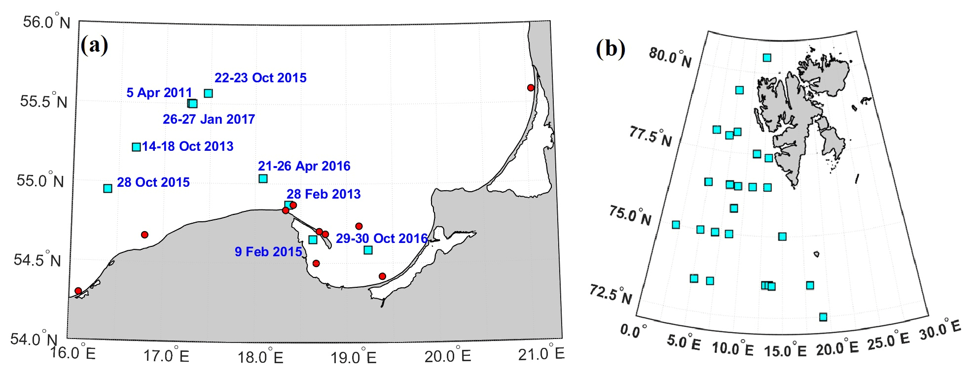
Figure 1 The flux measurement stations in the (a) Baltic Proper area and in the (b) North Atlantic Ocean. Stations marked in cyan indicate a long fetch and sea air mass conditions, which were used in the analysis. Points marked in red indicate a short fetch and land air mass advection, which were excluded from the analysis (these factors were obtained based on the HYSPLIT backward trajectories; see Appendix A).

2.1.2 The Baltic Proper

The Baltic Sea is one of the largest closed brackish seas. Fresh ocean deep-water inflows are rare (Rak, 2016). The wave fetch is much shorter than in the open ocean and depends on the wind direction and the upwind trajectories. That is why younger waves dominate in this environment (Lepparanta and Myrberg, 2009). As such, the Baltic Sea is characterized by different wave conditions (e.g., younger waves) compared to the open ocean.

In this study, 224 h of data gathered between 2011 and 2017 on 12 research cruises were used. The cruises were conducted mostly during late fall (October/November) and winter (January/February). Those periods were chosen due to the increased occurrence of high wind speeds. Main measurement stations from Baltic measurements are presented in Fig. 1a. Dates and positions of measurement stations are shown in Table A1.

2.1.3 North Atlantic Ocean

Measurements in the North Atlantic Ocean were conducted during summer. Aerosol measurements are included in the larger project, the so-called Arctic Experiment (AREX; Walczowski et al., 2017). The AREX cruises are annually organized 3-month-long Arctic research cruises on board RV Oceania and have occurred since 1986.

During these campaigns, multidisciplinary marine observations were conducted. The first part of each cruise was devoted to hydrological measurements. Aerosol concentration gradient measurements were carried out if meteorological and technical conditions were appropriate during each station (i.e., the station had to last more than 1 h, without occurrence of rain or fog). Despite difficult conditions, we succeeded in gathering a total of 56 h of measurements between 2009–2017 from six cruises. Aerosol measurement points during the AREX campaign are presented in Fig. 1b.

2.2 Instrumentation

For aerosol measurements, the optical particle counter CSASP-100-HV (CSASP) of the particle measurement system was used. The device counts aerosol particles in the diameter range 0.5 < D_p < 47 µm. In this study, 36 particle size bins were used for analysis. The sampling rate of the instrument was set up to 10 s. The detection limit of the device is 0.5 µm. The detailed technical specifications of this instrument are given in Appendix B.

Meteorological parameters, such as wind speed and humidity, were measured with a Vaisala meteorological probe at 10 m above the sea surface (WXT530). Humidity measurements were also verified at regular intervals using an Assmann psychrometer.

2.3 Gradient flux determination

To apply the gradient method, the CSASP was placed on a special lift on the starboard side of the ship. The lift allows one to change the height of the measurements between five levels: 8, 11, 14, 17, and 20 m. A single measurement on a single level lasts at least 2 min (with a 10 s sampling rate in each size range mode). After this time, the device was moved to the next level. Each flux was determined based on 30 min of vertical aerosol gradient measurements. The application of the method is presented in Appendix C, and a detailed description of the measurement methodology is given by Petelski (2003).

The net fluxes derived from the gradient method are affected by upward (emission) and downward (deposition) fluxes. This study focuses on the SSA emission, so all presented fluxes are emission fluxes and are labeled as F_N (flux of aerosol volume is marked as F_V). SSA emission fluxes were obtained based on the subtraction of modeled deposition fluxes from the net flux; in this respect, we used the Schack Jr. et al. (1985) model for deposition flux, as it has been tested for both Arctic waters (Nilsson et al., 2001) and the Baltic Sea (Nilsson et al., 2021). Due to the size range of the CSASP (> 0.5 µm D_p), the deposition flux from Schack Jr. et al. (1985) was dominated by impaction and sedimentation. All fluxes were reduced to 80 % equilibrium humidity using the approach of Fitzgerald (1975) updated with the recent sea spray growth factor given by Zieger et al. (2017). In this paper, all aerosol and flux spectra are presented in relation to reduced diameters, which are marked later as D_p@80 %: diameter at 80 % humidity.

2.4 External data sources

2.4.1 Reanalysis data

In this work, global atmospheric reanalysis (Hersbach et al., 2020) from the Copernicus platform was used. The parameters used are available with a 1 h temporal resolution and a spatial resolution of 0.5 × 0.5°. They include wind speed (U₁₀), significant wave height (H_S), spectral peak period (t_p), sea surface temperature (T_w), and air temperature (T_a).

For the Baltic region, wave data from the EU Copernicus Marine Service (Baltic Sea wave hindcast) were used. Wave data, such as significant wave height H_s and spectral peak period t_p calculated by the WAM model cycle 4.6.2, are available with 1 × 1^′ spatial resolution and with 1 h temporal resolution.

In order to obtain the same temporal resolution as fluxes (0.5 h), we interpolated all data for each half hour by averaging two known data points for each full hour.

Chlorophyll a (chl a) for the Atlantic Ocean, as an indicator of marine biological activity, was obtained from satellite data available in Global Ocean Colour (Copernicus-GlobColour; Garnesson et al., 1997).

Chl a data in the Baltic region were obtained from the SatBałtyk system (Satellite Monitoring of the Marine Environment in the Baltic Sea; Woźniak et al., 2011a, b), which is run by the Institute of Oceanology of the Polish Academy of Sciences. The chl a data are the product of satellite data (MODIS satellite) compiled with the EcoSat ecohydrodynamic model. The approach of data compilation is presented by Konik et al. (2019).

2.4.2 Back-trajectories

We established air mass backward trajectories, fetch, and time over the sea during measurements. To determine these, we used the HYSPLIT model (Stein et al., 2015) fed by the National Centers for Environmental Prediction Global Data Assimilation System (NCEP GDAS) 0.5 × 0.5° meteorological data; the back-trajectories were propagated for 24 h, reaching a final altitude of 10 m a.s.l. HYSPLIT outputs also embedded the mixing layer depth. All measurement time series with date, time, and duration are presented in Appendix A (Tables A1 and A2).

2.4.3 Secondary parameters

The meteorological and oceanographic parameters were compared with the SSA fluxes. Based on primary parameters (U₁₀, H_S, t_p, T_w, T_a), we also calculated secondary parameters, such as wind acceleration a_U, (Eq. 2), wave age (Eq. 3), wave Reynolds number (Eq. 5), and bulk atmospheric stability (also known as temperature difference between seawater and air: $T_{\mathrm{d}}=T_{\mathrm{w}}-T_{\mathrm{a}}$). In order to calculate water viscosity in ReH_w determination, we used seawater property library routines given by Nayar et al. (2016) and Sharqawy et al. (2010).

2.5 Error propagation

Measurement uncertainty values were calculated according to general rules of error propagation (i.e., Taylor, 2012). The absolute uncertainty of the particle counter can be obtained from Poisson's distribution properties, which is the standard deviation ${\mathit{\sigma }}_{\mathrm{P}}=\sqrt{\mathit{\mu }}$, where μ is the mean concentration value. The relative uncertainty can be defined as δ_p= ${\mathit{\mu }}^{\mathrm{1}/\mathrm{2}}/\mathit{\mu }$ so it is inversely proportional to the mean particle concentration (in our case, the single measurement was 10 s). By taking into account mean values from our measurements, we obtained Poisson error values between 0.02 % for the lower aerosol channel (0.5–1.0 µm) and 15.68 % for the last channel (44.0–47.0 µm). Such values are in a similar range to other OPCs available on the market (i.e., TSI 3340 LAS, Grimm OPC 1.109). We present detailed relations between δ_p and the size distribution of the OPC in Fig. C2.

The uncertainty of wind speed measured by acoustic anemometer, according to the manual, is below < 1 %. The uncertainty of the data taken from the WAM model is estimated as follows: ΔU₁₀≈ 10 %, ΔH_s≈ 2 %–5 % after Janssen et al. (2007), and Δω_p≈ 15 % after Abdalla et al. (2010).

The uncertainty of the fitting N_* parameter can be obtained from absolute uncertainty of the least-squares method:

$$\begin{array}{}\text{(6)}& {\displaystyle }{\mathit{\sigma }}_n=\sqrt{{\displaystyle \frac{\mathrm{1}}{l-\mathrm{2}}}{\sum }_{i=\mathrm{1}}^l{\left(n_i-C-N_{*}\ln \left(z\right)\right)}^{\mathrm{2}}}\text{(7)}& {\displaystyle }{\mathit{\sigma }}_{N_{*}}={\mathit{\sigma }}_n\sqrt{{\displaystyle \frac{l}{l\sum \ln {\left(z\right)}^{\mathrm{2}}-{\left(\sum \ln \left(z\right)\right)}^{\mathrm{2}}}}},\end{array}$$

where l= 5 (number of measurement levels), ln(z) is the natural logarithm of measurement height, and n_i is a single measurement on each level. For different values of the correlation coefficient r of the fitting, relative uncertainty (defined as ${\mathit{\sigma }}_{N*}{N}_{*}^{-\mathrm{1}}$) was checked. For r values in the range of 1.0 < r < 0.5, uncertainty was lower than 7 %. For worst fitting (r < 0.5), the relative uncertainty increases drastically (for r= 0.2, even 30 %). Lower values of r imply that the aerosol concentration gradient did not exist, so it is impossible to consider the aerosol gradient flux. As such, data with correlations lower than 0.4 were excluded from further consideration.

Based on these considerations, the total uncertainty of the flux measurements varied between 7 % and 17 %. In Fig. C2, we present detailed total uncertainty vs. size distribution of the CSASP.

3 Results and discussion

3.1 Flux overview

A histogram of total fluxes F_N is presented in the Appendix (Fig. A1), from which it is clear that positive (emission) fluxes dominated in both Baltic and Atlantic data. The peak for the Baltic Sea fluxes at 5 % of total frequency occurrence have a median value M_F= 3.4 × 10⁴ m⁻² s⁻¹ (mean value μ_F= 8.9 × 10³ m⁻² s⁻¹) and standard deviation σ_F= 6.8 × 10⁵ m⁻² s⁻¹. For the Atlantic dataset, the peak of occurrence is at 14 % of cases with a median value M_F=4.0 × 10⁴ m⁻² s⁻¹ (mean value μ_F=1.0 × 10⁴ m⁻² s⁻¹) and σ_F=2.7 × 10⁵ m⁻² s⁻¹. The significantly higher fluxes measured in the Atlantic dataset are explained by the fact that, during ocean measurements, we deal with high fetch and a lack of air mass advection from land. In the Baltic Sea cases, measurements with land advection (according to the 24 h backward trajectories) were excluded from further analysis.

To avoid the influence of air mass advection from land, the measurements were divided into two groups according to surface conditions derived from 24 h backward trajectories (see below Sect. 3.5.2): (1) entirely marine during the last 24 h and (2) some marine during the last 24 h, with land influence. For marine conditions, the estimated fetch varied between 110 and 350 km. The times over the sea for marine conditions varied from 6 to 20 h.

3.2 Overall data trends

In order to present the large data trends in a compact way, we use the following exponential fits to describe the relationship between the total aerosol fluxes and wind speed, wave age, wave height, and wave Reynolds number:

$$\begin{array}{}\text{(8)}& P\left(x\right)=\exp \left(a{x}^b\right).\end{array}$$

The relationship between wind acceleration and aerosol number flux can be described with the following exponential relationship:

$$\begin{array}{}\text{(9)}& G\left(x\right)=\exp \left(ax+b\right).\end{array}$$

The relationship between temperatures and aerosol number flux can be described with the following linear relationship:

$$\begin{array}{}\text{(10)}& L\left(x\right)=ax+b,\end{array}$$

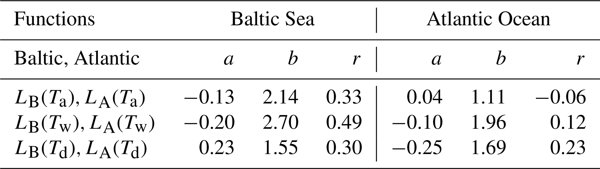
where x stands for a chosen parameter. The fitting results with the functional parameters a and b are presented in Tables 1 and 2. The first two functions, P(x) and G(x), were used for the total fluxes. The third group of functions L(x) was fitted to fluxes which were normalized by a wind speed relation:

$$\begin{array}{}\text{(11)}& F_{\mathrm{S}}=F_N/P_{\mathrm{B}}^{\mathit{\beta }}\left(U_{\mathrm{10}}\right).\end{array}$$

The resulting coefficients of this parameterization are presented in Table 3.

Tables 1–3 also contain the squared correlation coefficient. We can note a strong correlation between the total aerosol flux and U₁₀ at low chl a and between the total aerosol flux and ReH_w.

Table 1 Parameterization results between several ambient factors and the total aerosol fluxes from the Baltic Sea: wind speed U₁₀, wind acceleration a_U, wave age $c_{\mathrm{p}}/U_{\mathrm{10}}$, wave Reynolds number ReH_w, and significant wave height H_s. The parameterization coefficients a and b are based on Eqs. (8), (9), and (10), and r represents the fitting correlation. Additional subscripts indicate the following: “B” is the fit to the Baltic Sea data, “α” is the fit to the whole range of chlorophyll a concentrations, “β” is the fit to data in the range below 3.5 mg m⁻³ of chl a, and “v” is the fit to volume flux data.

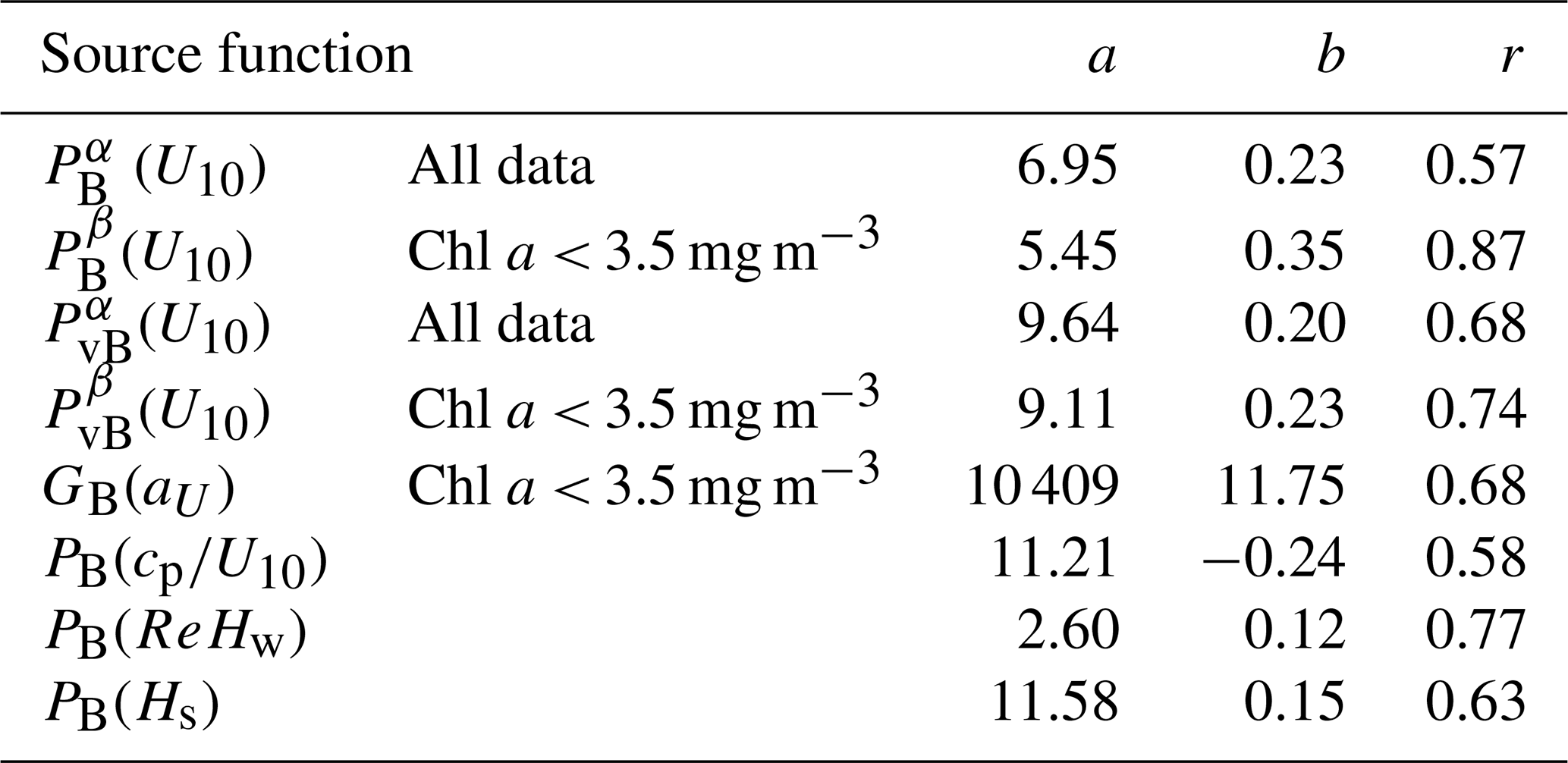
Table 2 Parameterization results between factors and total aerosol fluxes from the Atlantic Ocean. The analyzed parameters are the same as in Table 1. The subscript “A” indicates fit to the Atlantic Ocean data.

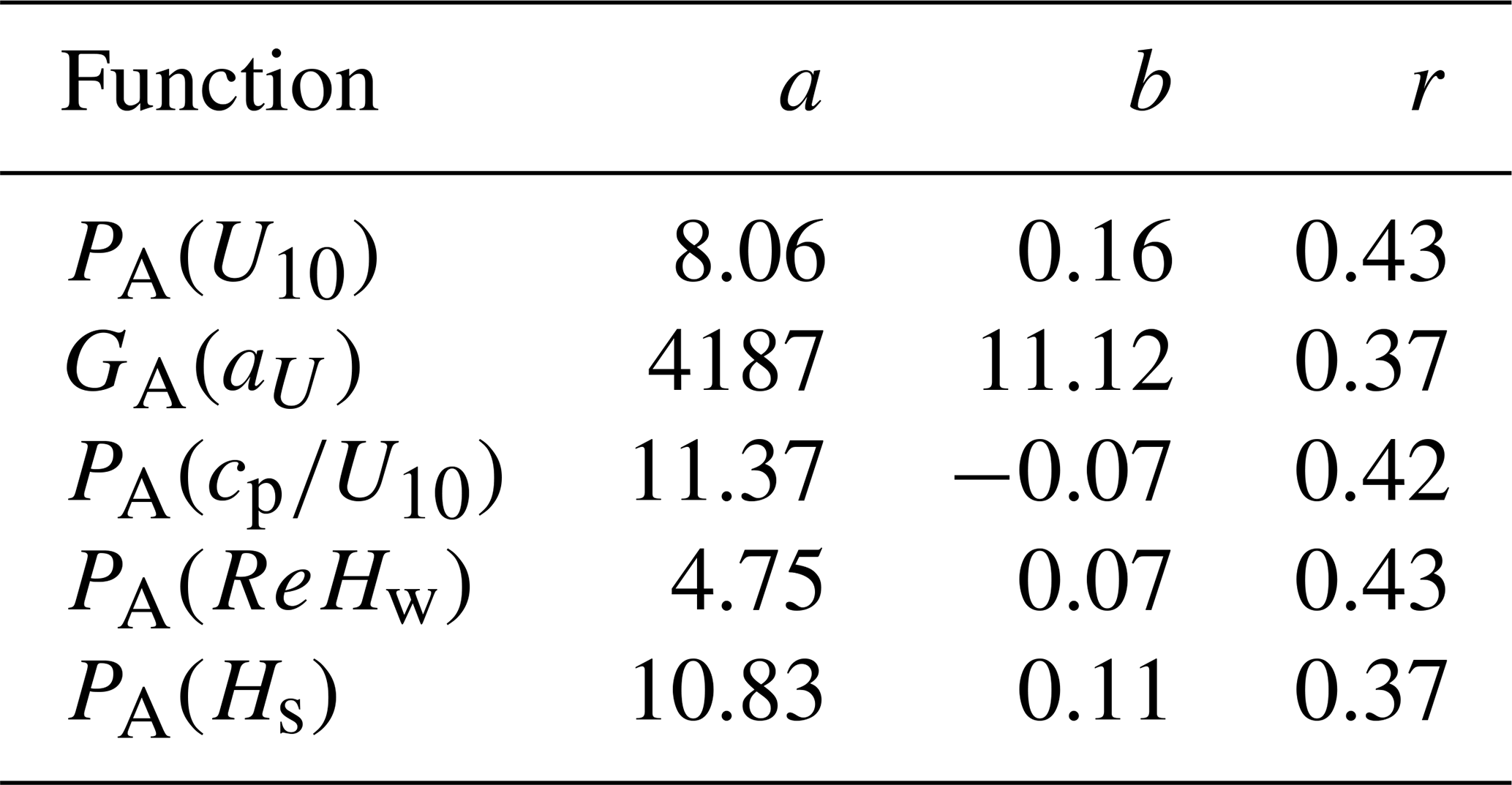
Table 3 The fitting coefficients of functions fitted to all wind-speed-normalized aerosol fluxes according to Eq. (11).

3.2.1 The impact of marine biological activity on sea spray fluxes

Based on the findings by Nilsson et al. (2021), who reported a weakened wind dependency when organics were present, we could expect influences of biological activity in the seawater on sea spray formation. Some of our measurements in the Baltic region were also carried out during early summer and fall, the typical periods of algae bloom in the Baltic Sea. In contrast, our Atlantic measurements were carried out entirely during the summer season. For this reason, we chose to employ chl a as a proxy for marine biological activity. From here on, we use superscript α to denote the entire dataset and superscript β for chl a < 3.5 mg m⁻³.

In the Baltic Sea, the chl a varied between values of 0.23 and 4.28 mg m⁻³. In the Atlantic Ocean measurements, the minimum chl a concentration was 0.13 mg m⁻³ and the maximum was 2.20 mg m⁻³. These numbers are within the range of typical seasonal mean values (Stoń-Egiert and Ostrowska, 2022). The upper range also compares well with the Baltic EC flux data by Zinke et al. (2024), with averages of 3.9 and 5.2 mg m⁻³ for the May and August field campaigns, respectively.

In Fig. 2 we present interrelations between total SSA fluxes, wind speed, and water chl a concentration in the Baltic Sea. To indicate the impact of chl a, we fitted four curves to our dataset, assigned respectively as $P_{\mathrm{B}}^{\mathit{\alpha }}(U_{\mathrm{10}}$), $P_{\mathrm{B}}^{\mathit{\beta }}(U_{\mathrm{10}}$), $P_{\mathrm{vB}}^{\mathit{\alpha }}(U_{\mathrm{10}}$), and $P_{\mathrm{vB}}^{\mathit{\beta }}(U_{\mathrm{10}}$), with dashed red lines for the entire dataset (upper index α) and dotted blue lines for low chl a below 3.5 mg m⁻³ (upper index β). The first two functions were fitted to number flux, and the second two were fitted to volume flux (as indicated by the additional subscript “v”). The curve coefficients are specified in Table 1.

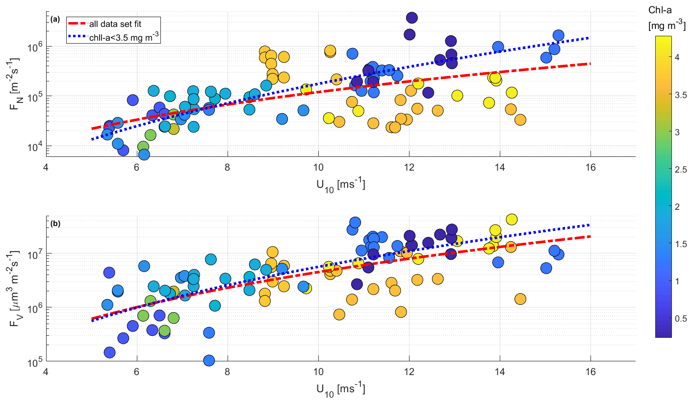
Figure 2 The influence of 10 m wind speed and chlorophyll a concentration in water on sea spray fluxes over the Baltic Sea. (a) Aerosol number flux. (b) Aerosol volume flux.

All measurements at higher chl a concentration were made in the open-sea region (5 May 2011, 18 October 2013, 23 October 2015, and 22 April 2016; details with mean values are presented in Table A1). All these high chl a measurements were made in the open-sea region without any fresh water inflow from rivers that might have affected the measurements. This is also reflected in the constant salinity values across all stations.

In the wind range 8.5–10.5 m s⁻¹, we observed higher aerosol emissions at chl a > 3.5 mg m⁻³ compared to lower chl a concentrations, while, at higher wind speeds (10.5–14.5 m s⁻¹) with high chl a, we observed aerosol fluxes almost 1 order of magnitude lower than in the case of low chl a concentrations. This effect is less pronounced if we investigate the SSA volume fluxes (Fig. 3b), which suggest that smaller particles were mostly associated with higher emission. We did not observe such an effect on the fluxes measured in the Atlantic Ocean.

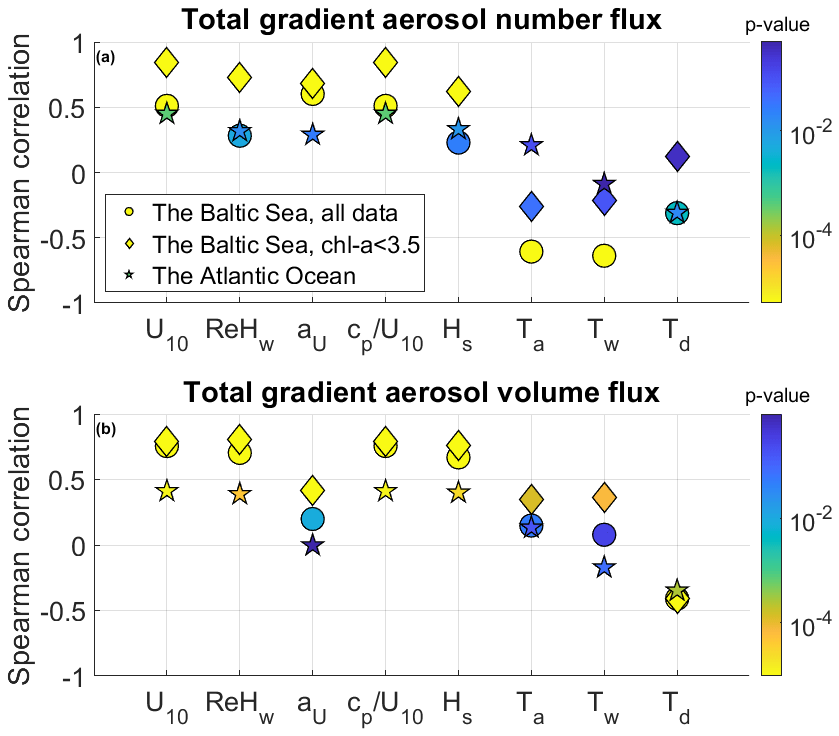
Figure 3 Spearman correlations calculated between measured aerosol fluxes and investigated parameters (wind speed U₁₀, wave Reynolds number ReH_w, wind acceleration a_U, wave age $c_{\mathrm{p}}/U_{\mathrm{10}}$, wave height H_s, air temperature T_a, and water temperature T_w. In panel (a) we present number flux correlations, and in panel (b) we present volume flux correlations. Circles represents correlations in the Baltic Sea in all chl a conditions, diamonds represent correlations in the Baltic Sea in low chl a conditions, and stars represent correlations in the Atlantic Ocean. Instances of statistical significance are presented as p-values with colors. Blue represents low p-values (where the correlation is statistically significant), green is the boundary of the statistical significance level, and yellow indicates high p-values (where the correlation is insignificant).

To statistically prove the difference between the fits to the low and high chl a regimes ($P_{\mathrm{B}}^{\mathit{\alpha }}(U_{\mathrm{10}}$) with $P_{\mathrm{B}}^{\mathit{\beta }}(U_{\mathrm{10}}$) and $P_{\mathrm{vB}}^{\mathit{\alpha }}(U_{\mathrm{10}}$) with $P_{\mathrm{vB}}^{\mathit{\beta }}\left(U_{\mathrm{10}}\right))$, we applied several statistical tests (all test results are presented at the 5 % significance level). Since the variances of analyzed datasets are not equal, we have to use the so-called unequal variances t test (Welch's t test, which is the generalization of the classical t test). A detailed summary of the test results is provided in Table D1.

In terms of number flux, the low and high chl a regimes were statistically different (p= 0.0094), while, in terms of volume flux, the difference was not significant (p= 0.13). This finding implies that the emission of smaller submicrometer particles (which contribute to number concentration) was more affected by chl a than bigger supermicrometer particles (which contribute to aerosol volume).

We also employed the right-tailed Welch's test in order to investigate in detail the difference between curves $P_{\mathrm{B}}^{\mathit{\alpha }}(U_{\mathrm{10}}$) and $P_{\mathrm{B}}^{\mathit{\beta }}(U_{\mathrm{10}}$). The fits were segregated into a low wind speed range (below 10 m s⁻¹) and a higher wind speed range (above 10 m s⁻¹). In the case of low wind speeds, the right-tailed Welch's test proved that there was no significant difference between both fits (p= 0.32). However, at high wind speeds they were significantly different (p= 5 × 10⁻⁴).

The above results show that number concentration flux from waters with a higher chl a was decreased in higher wind speed regimes in comparison with low chl a concentrations. This finding suggests that biological activity indicated by chl a may have a suppressing effect on aerosol number flux. The cause of flux decrease for higher organic activity may be caused by changes in surface tension which affect the bubble properties, such as bubble film thickness and lifetime (Sellegri et al., 2021; Barthelmeß and Engel, 2022).

However, we did not observe a dampening effect for the volume flux, which is mostly affected by bigger particles. This result relates to previous studies, which reported that submicron particles emitted from the sea surface are mostly enriched with organic matter, while supermicron particles mainly consist of inorganic sea salt (Keene et al., 2007; Yoon et al., 2007; Facchini et al., 2008; Quinn et al., 2014). For this reason, we should not expect a significant influence on the gradient aerosol volume flux from organic sea spray in the supermicrometer range of the CSASP-100-HV used in this study, and we should expect only limited influence in the submicrometer range, since it is limited to > 0.5 µm D_p.

Nonetheless, Nilsson et al. (2021; Fig. 9) reported that, while the EC flux of sea salt particles had a log-linear fit between log10(F_n) and U₁₀ with a slope of 0.11 and a correlation of r= 0.74, the EC flux with organic sea spray included only gave a slope of 0.02 and a correlation of r= 0.23. Hence, the presence of organic compounds in the sea spray aerosol decreases SSA emissions and at the same time increases the scatter of the data points, lowering the correlation. This is in good agreement with Fig. 2, especially the gradient aerosol number flux in Fig. 2a, where the slope decreases significantly when high chl a data points are included and the scatter between data points increases.

3.2.2 Parameter correlations with sea spray emission

In Fig. 3 we present Spearman's correlations between measured total fluxes (Fig. 4a) and volume fluxes (Fig. 4b) with analyzed parameters, with statistical significance expressed as p-values.

As described above, we have split the Baltic Sea measurements into two categories: data with low chl a concentrations (chl a < 3.5 mg m⁻³; see Fig. 4a) and all data. We treat the Atlantic Ocean data as a third category, where chl a was always lower than in the Baltic Sea data (Atlantic chl a = 0.60 ± 0.58 mg m⁻³). We observed the highest statistically significant (p-value < 0.05) positive correlations (r_s > 0.6) between the gradient aerosol fluxes and U₁₀ and wave state parameters at low chl a conditions in the Baltic Sea.

The effect of biological activity in the Baltic Sea region reduces the correlation of wind and wave parameters with aerosol fluxes, which is in agreement with Nilsson et al. (2021). The influence of biological activity hence weakens the effect of increasing U₁₀. This is why, for the remaining analysis, we decided to present the effect of U₁₀ and wave state by analyzing only aerosol gradient fluxes with low chl a.

In middle- and high-latitude meteorological data, the correlation between wind speed and temperature is usually high because cold periods are usually associated with higher wind speed and vice versa, on both a seasonal and a synoptic timescale. Likewise, sea surface temperature and the temperature of the atmospheric surface layer are usually highly correlated. In order to eliminate the influence of wind speed on our data, which may interfere with temperature effects, we calculate correlations between normalized aerosol fluxes and temperature parameters (T_a, T_w, and T_d). We implemented a normalization by dividing measured fluxes by the obtained wind-speed-related function (details in Sect. 4.3.3).

For the effect of temperature, we observed a more complex picture. We found that T_a and T_w have a negative statistically significant correlation (r_s < −0.5, p-val < 10⁻¹¹) with all chl a cases of the Baltic aerosol number fluxes (Fig. 3a). The remaining calculated correlations (cases of low chl a in the Baltic Sea and Atlantic Ocean) were insignificant (and also negative, apart from T_d in the Atlantic Ocean cases). We obtained the opposite results when analyzing the aerosol volume flux. In this case, T_a and T_w correlated positively with Baltic Sea gradient aerosol volume fluxes limited to low chl a conditions. The correlations were not high (r_s ∼ 0.4), but they were significant in both cases (p-val < 0.05). The cases of high chl a correlations were insignificant for T_a and T_w. We also obtained statistically significant negative correlations between aerosol gradient volume fluxes and T_d in all three datasets.

3.2.3 Dependence of sea spray fluxes on horizontal wind speed

An exponential increase in the total SSA number flux was observed with increasing horizontal wind speeds and wind acceleration for both the Baltic Sea and Atlantic Ocean measurements (see Fig. 4).

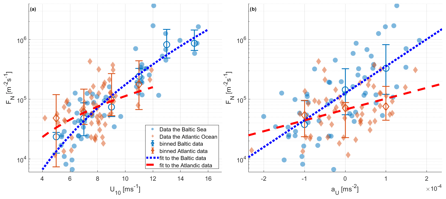
Figure 4 Total aerosol fluxes versus wind speed (a) and wind acceleration (b). Error bars represent the first and third quantile of each data bin (25 %–75 %), with a median value (50 %). Fitting coefficients are presented in Table 1.

SSA fluxes were categorized based on wind speed classes, each having a bin width of 2 m s⁻¹. Aerosol gradient fluxes measurements were carried out over the Baltic Sea between 2.1 and 15.8 m s⁻¹ and in the Atlantic Ocean between 2.1 and 11.9 m s⁻¹.

For each wind speed class, we present median and percentile 25 %–75 %, with empty circles for the Baltic Sea data and empty diamonds for the Atlantic Ocean data and error bars. We used the same convention for all total flux comparisons with other parameters.

Size-resolved aerosol gradient fluxes binned according to these wind speed classes are presented in Fig. 5. In the Baltic Sea, we can see a systematic increased emission of particles from 0.25 µm < D_p < 2 µm. For aerosols with D_p > 2 µm, the pattern is different: in the highest wind speed class (15 m s⁻¹), we observed a small decrease in the emission fluxes compared to 11 m s⁻¹.

In Fig. 5b, we present aerosol gradient flux size distributions in wind speed classes present in the Atlantic Ocean data (there was no U₁₀ in the 15 m s⁻¹ range in the Atlantic Ocean dataset). In this case, the increase in fluxes with wind speed was smaller, which is also visible if we compare the slopes of the fitted curves in Fig. 4a. We can also observe that, in lower wind speed classes, the measured Atlantic Ocean emission aerosol gradient fluxes were higher than over the Baltic Sea, by factors of 3.0 for 5 m s⁻¹ and 1.7 for 7 m s⁻¹. The highest U₁₀ range present in both datasets and in both Fig. 5a and b (11 m s⁻¹) are relatively similar, so the smaller increase in sea spray emissions over the Atlantic Ocean with increasing U₁₀ is due to higher fluxes at the lowest wind speeds.

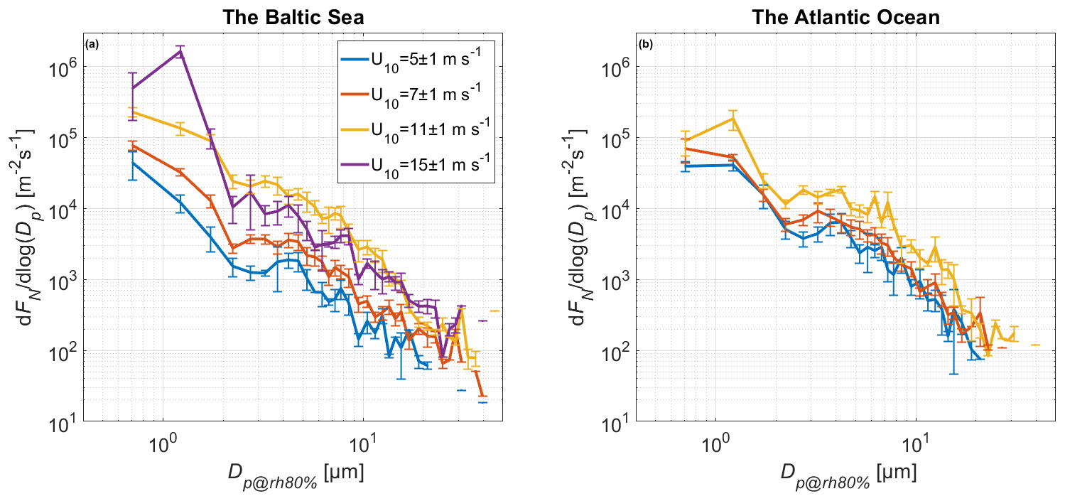
Figure 5 Measured mean sea spray aerosol number gradient flux spectra reduced to 80 % relative humidity in relation to wind speed binned in wind speed classes (U₁₀). Error bars indicate 1 standard error. (a) Over the Baltic Sea. (b) Over the Atlantic Ocean. The highest wind speed range (U₁₀= 15 m s⁻¹) is absent in the Atlantic Ocean dataset. No U₁₀ < 4 m s⁻¹ is included, since we do not expect breaking waves in this wind speed range.

3.2.4 Dependence of sea spray fluxes on horizontal wind acceleration

The wind acceleration varied from minimum values of −2.0 × 10⁻⁴ m s⁻² (over the Baltic Sea) and −2.3 × 10⁻⁴ m s⁻² (over the Atlantic Ocean) up to maximum values of 1.8 × 10⁻⁴ and 1.7 × 10⁻⁴ m s⁻². In this case, we assumed only three classes: decreasing wind speed (a_u < −2.5 × 10⁻⁵ m s⁻²), increasing wind speed (a_u > 2.5 × 10⁻⁵ m s⁻²), and near-constant wind speed (−2.5 × 10⁻⁵ < a_u < 2.5 × 10⁻⁵ m s⁻²).

Over the Baltic Sea, the measured aerosol gradient flux size distributions for increasing U₁₀ conditions are higher for decreasing wind conditions in sizes up to diameters of 16 µm. For larger particles, the difference between these two classes is much smaller and less significant (overlapping each other's error range). We did not observe any difference between these two classes over the Atlantic Ocean. The reason for that may be the lack of U₁₀ > 12 m s⁻¹ (and hence fewer wind speed accelerations), which does not let us observe enough variability.

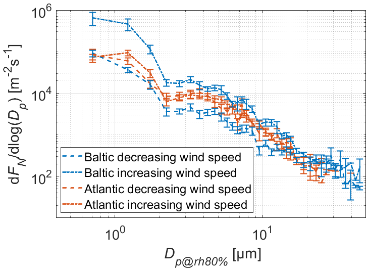
Figure 6 Aerosol number sea spray gradient flux size distribution in relation to the wind acceleration parameter a_u. The size spectra present mean values over the Baltic Sea and Atlantic Ocean for two cases: increasing U₁₀ (a_u > 2.5 × 10⁻⁵ m s⁻²) and decreasing wind speed U₁₀ (a_u < 2.5 × 10⁻⁵ m s⁻²).

This is opposite to the total aerosol fluxes (0.11–6 µm D_p) reported by Yang et al. (2019), which are larger for decreasing U₁₀ than for increasing U₁₀. In the current study, this could be explained by larger H_s during decreasing wind speeds. This is also opposite to the wind history effect on W presented by Stramska and Petelski (2003) and Callaghan et al. (2008), which showed that W was larger for the same wind speed when the wind speed was decreasing than when it was increasing, but only for U₁₀ > 10 m s⁻¹. This dataset was from a ship cruise in the northeastern Atlantic Ocean, so it should be more comparable to our Atlantic dataset. We are not aware of any whitecap wind history study in the Baltic Sea.

3.2.5 Wave state parameters

For the Baltic Sea cruises, it was possible to gather a wide range of wave heights ranging from 0.1 to 3.7 m. The corresponding peak period ranged from 1.5 to 9.3 s. In the Atlantic Ocean region, the H_s value varied in the range of 0.7 to 2.2 m. Peak-period values were in the range of 4.7 to 8.2 s.

With increasing wave age, we observe an exponential decrease in total aerosol production (see Fig. 7a). In the Baltic area, our SSA gradient flux observation covered wave ages in the range of 0.46 < $c_{\mathrm{p}}/U_{\mathrm{10}}$ < 1.87. In the Atlantic Ocean region, there were no younger waves; therefore, observations covered wave ages in the range of 0.81 < $c_{\mathrm{p}}/U_{\mathrm{10}}$ < 8.23. Measurement points were combined in wave age classes with a bin width of 0.5: three classes for the Baltic Sea data and six classes for the Atlantic data.

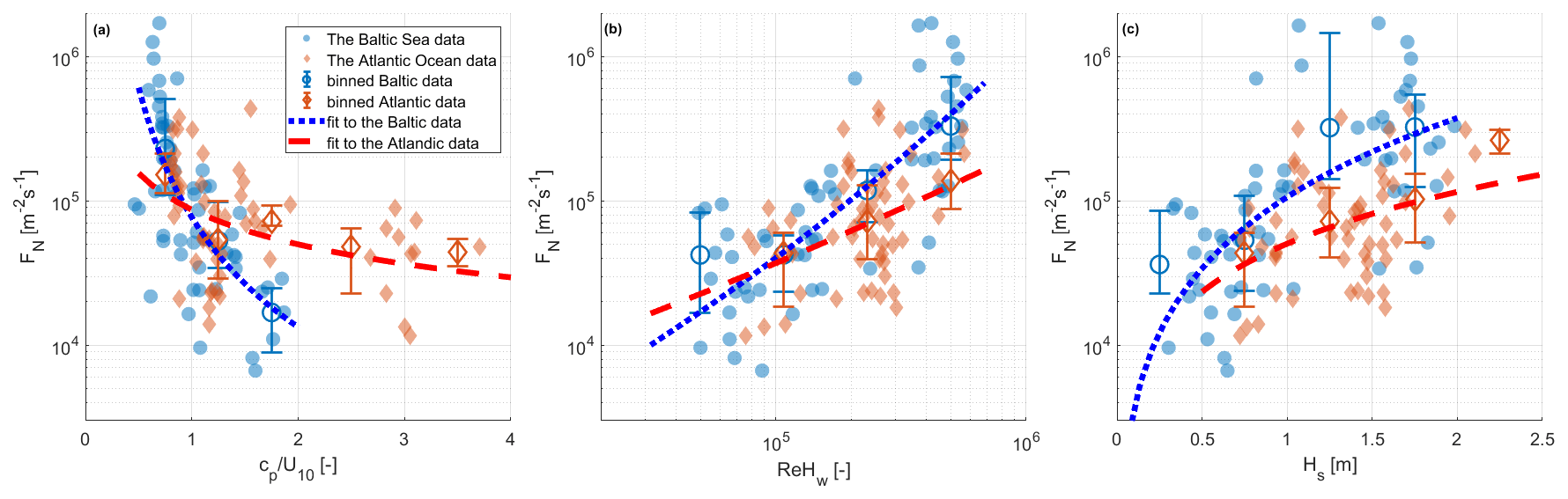
Figure 7 Total aerosol number gradient fluxes depending on wave age (a), wave Reynolds number ReH_w (b), and wave height H_s (c). Error bars represent the first and third quantile of each data bin (25 %–75 %), with a median. Fitting coefficients are presented in Table 1.

We can see a constant decrease in the aerosol flux with the wave age in both datasets. We observed a much more rapid decrease in the total gradient aerosol flux over the Baltic Sea than over the Atlantic Ocean and a $c_{\mathrm{p}}/U_{\mathrm{10}}$ span over a wider range with higher values.

Both datasets were binned into four bins of ReH_w (Fig. 7b). We observed a linear increase in the total aerosol gradient number flux with increasing ReH_w over both the Baltic Sea and the Atlantic Ocean. This increase was steeper over the Baltic Sea. In the highest bin of the Reynolds number (mean ReH_w= 5 × 10⁶), we observed higher aerosol flux in the Baltic Sea than over the Atlantic Ocean. Yang et al. (2019) presented total aerosol EC fluxes (0.11–6 µm D_p) as a function of H_s, and for their open-sea data they derived a linear relationship for H_s < 1 m and EC fluxes < 10⁴ m⁻² s⁻¹. Zinke et al. (2024) presented a total aerosol EC flux (0.25–2.5 µm wet diameter) as a power law function of H_s, where the slope was 0.05 and the power was 2.2. The aerosol EC fluxes were < 3 × 10⁵ m⁻² s⁻¹ and H_s < 2 m. Yang et al. (2019) noted that ReH_w failed to reconcile their EC aerosol fluxes with those of Norris et al. (2013), and we can now conclude that neither study reconciles this dataset, or that of Zinke et al. (2024), with these sea spray fluxes.

Figure 7c shows the total aerosol gradient fluxes binned according to wave height H_s with a bin width of 0.5 m. We observed an SSA flux increase with increasing H_s, which was also reported by Yang et al. (2019) and Zinke et al. (2024). They have aerosol EC fluxes of higher magnitudes than our gradient aerosol fluxes because their measurements included smaller aerosol particles. Zinke et al. (2024) reports a linear fit between aerosol EC emission fluxes with a slope of 1.68 × 10⁻⁷. Yang et al. (2019) presented an exponential fit, with unknown slope. The curves fitted to our data were exponential power laws, where the slope was 2.60 and the power was 0.12.

3.2.6 Temperature and atmospheric stability

We further investigated the impact of air and seawater temperatures on the aerosol emission flux. The air temperature oscillated in the Baltic Sea from −3.2 to 13.3 °C and in the Atlantic Ocean from 1.2 to 8.4 °C. The water temperature in the Baltic Sea was between 1.6 and 13.1 °C, and it was between 2.3 and 8.4 °C in the Atlantic Ocean. We also used the temperature difference between sea surface temperature and air temperature at 2 m a.s.l. ($T_{\mathrm{d}}=T_{\mathrm{w}}-T_{\mathrm{a}}$) as an indicator of atmospheric stability. These values varied from −2.6 to 4.8 °C in the Baltic Sea and from −0.5 to 4.0 °C in the Atlantic Ocean region.

Due to a correlation between temperature and wind speed, a direct correlation between aerosol gradient fluxes and temperature could be biased. The reason is the strong, high correlation between T_a and U₁₀ on both seasonal and synoptic timescales (higher air temperatures correlate with lower wind speeds and vice versa). That is why, in order to exclude the effect of U₁₀, we normalized fluxes by our source function expression $P_{\mathrm{B}}^{\mathit{\beta }}$ (U₁₀). The normalized fluxes, in relation to T_a,T_w, and T_d, are presented in Fig. 8.

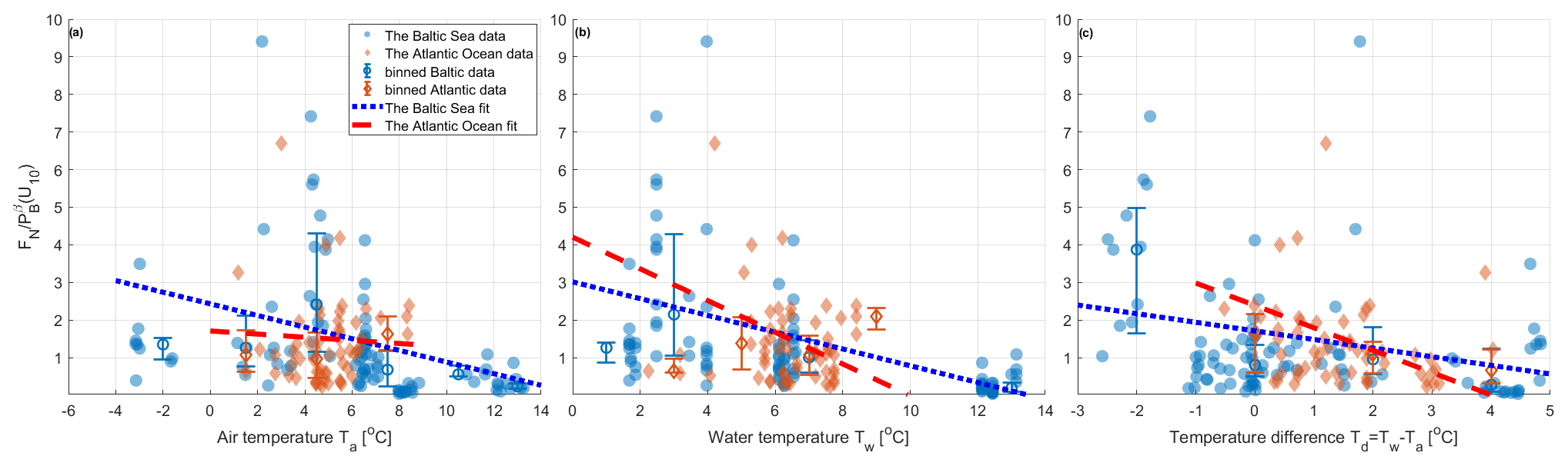
Figure 8 Total sea spray aerosol gradient fluxes normalized by the wind-speed-dependent source function $P_{\mathrm{B}}^{\mathit{\beta }}$ (U₁₀) (Eqs. 8 and 11) as a function of air temperature T_a, water temperature T_w, and temperatures difference T_d. We fitted the functions according to Eq. (10). The fitting coefficients are presented in Table 3.

As we can see in Fig. 3 and Table 3, the Spearman's correlations of wind-normalized fluxes with T_a and T_d are lacking significant aerosol volume flux correlations. In the case of aerosol gradient number fluxes, we observed negative correlations (statistically significant only in the case of all Baltic Sea chl a values), and only for T_w (r²= 0.24), using a linear fit with a negative slope of −0.20; see Table 3. In the case of volume fluxes, we observed positive correlations (statistically significant only for the low chl a case; see Fig. 3).

The decrease in sea spray emission gradient fluxes with increasing T_w is consistent with studies which report the suppression of SSA emission with increasing T_w (see references in the Introduction and compare also with Fig. 3). It is worth noting that our Baltic Sea dataset, which spans T_w= 1.6 to 13.1 °C, covers exactly the T_w range (from −2 to about 12–15 °C) in which Salter et al. (2014) and many others have observed the largest decrease in submicrometer sea spray production. The narrower T_w range in the Atlantic dataset (2.3 to 8.4 °C) may not be enough to distinguish this trend. The fact that we observe it only for the total aerosol number gradient flux is logical, since this should be dominated by the submicrometer aerosol particles, while we do not see a clear trend in the total aerosol volume gradient fluxes, since these are likely dominated by supermicrometer particles.

As discussed in the Introduction, for the supermicrometer sea spray, some studies show an increase in sea spray emissions with increasing T_w (Liu et al., 2021), so, in this case, our results also support this finding. Based on that, we speculate that we observed two different phenomena (just like Bowyer et al., 1990). An increase in T_w suppresses the emission of submicron particles but increases the emission of supermicrometer mode. This leads to a decrease in SSA number but an increase in SSA volume with increasing T_w.

The higher aerosol gradients observed under stable atmospheric conditions are likely caused by increased stratification and suppression of turbulent mixing and dispersion. In the case of stable atmosphere, turbulent eddies were smaller and less energetic, so particles reached lower heights, which caused us to observe a higher gradient flux. As we can see, our data source fittings have low correlations. Large data scatter suggests that many effects interact in these observations. Further research is needed to disentangle the different factors impacting SSA fluxes.

3.3 Comparison with relevant source functions

We decided to choose several different source functions for comparison with our datasets. In order to compare wind speed dependence, we used three functions determined by in situ measurements: f_pet from Petelski and Piskozub (2006) with improvements by Andreas (2007), f_sm from Smith et al. (1993), and f_zin from Zinke et al. (2024). The f_zin function is the only one specifically derived for the brackish seawater of the central Baltic Sea and is therefore relevant for part of our dataset. We also used two functions determined in tank experiments, f_mar from Mårtensson et al. (2003) and f_sal from Salter et al. (2015), because they are currently the only ones available that depend on T_w, and we used one general source function used in the Norwegian Earth System Model (NorESM) – f_kir from Kirkevag et al. (2013) – which is a modification of the Mårtensson et al. (2003) function adapted to the modal aerosol model in NorESM by Struthers et al. (2011). In Fig. 9, we can see the relatively good comparisons of source functions with our measurement flux spectra in two wind speed classes.

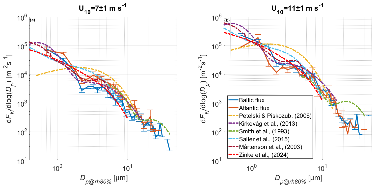
Figure 9 Comparison of our measured sea spray aerosol number gradient flux size spectra with selected sea spray generation functions in relation to two different wind speed cases: (a) 7 m s⁻¹ and (b) 11 m s⁻¹. For the source parameterizations by Mårtensson et al. (2003), Struthers et al. (2011)/Kirkevåg et al. (2013) and Salter et al. (2015) used T_w= 6.34 °C.

As evident in Fig. 9, the related f_kir and f_mar functions in particular (originating from the same laboratory data) reproduce our observations very well. The fit is decent for both submicrometer particles and in the coarse particle range (D_p > 2 µm). It is also worth noting that the shape and location of the modal distribution agree with the results obtained. The f_sal and f_zin functions also reproduce the order of magnitude of SSA emission fluxes well. For these functions, a clear overestimation of the SSA emission fluxes in the aerosol size range from 1 to 4 µm D_p is visible.

The f_sm function, which is the oldest of the selected parameterizations dedicated to the largest aerosol particles (valid for D_p@rh80 > 6 µm; see Appendix A of de Leeuw et al., 2011), reproduces the emissions well in the range of 5 to 15 µm. For larger particles, the function predicts the existence of another aerosol mode associated with spume droplets. We did not observe the predicted increase in emission in this range. This is due to the fact that, in order to perform accurate emission measurements in this size range, longer measurement times are necessary to collect enough of the spume droplets, which have a very small atmospheric number concentration. This is beyond the scope of our study.

We further compared the dependence of aerosol fluxes on the wave Reynolds number observed in this study to parameterizations by Ovadnevaite et al. (2014) and Zinke et al. (2024), assigned as f_ova and f_zinRe (Fig. 10).

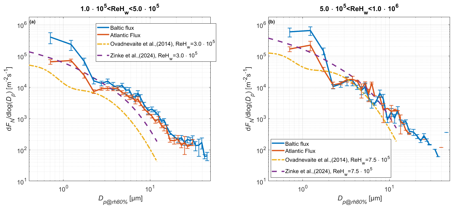
Figure 10 Comparison of measured sea spray aerosol number gradient flux size spectra as a function of D_p (at 80 % relative humidity), with selected sea spray generation functions related to two different wave Reynolds numbers.

As can be seen in Fig. 10, the f_ova function underestimates the aerosol emission, especially for the submicron mode (D_p < 2 µm). With increasing ReH_w values (Fig. 10b), the f_ova function much better reproduces the emission for larger particles (D_p > 1.5 µm). In the case of the f_zinRe function, we observe a good agreement with the Atlantic fluxes. The differences between the source functions and the measurements in the range of ∼ 1.7 to ∼ 3.2 µm are largely due to the different modal characteristics of the fits.

In Fig. 11, we compare the chosen source functions with our measurement data as a function of U₁₀, H_s, and ReH_w. The source functions were integrated over the size distribution range of this work (0.5 µm < D_p < 47 µm).

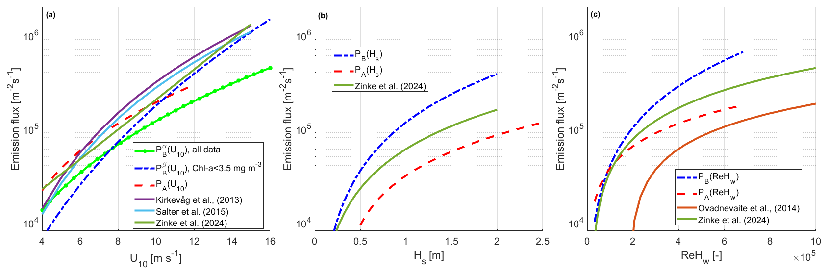
Figure 11 Comparison of the parameterizations presented in this work with selected literature source functions: wind speed in panel (a), significant wave height in panel (b), and Reynolds number in panel (c).

For U₁₀ < 8 m s⁻¹, the P_A(U₁₀) function (the Atlantic emissions) shows a good agreement with the other source functions. For larger wind speeds, the discrepancy increases due to the different slope of the curve compared to the other models. The $P_{\mathrm{B}}^{\mathit{\beta }}$ function (low chl a concentrations) is characterized by a similar slope to the compared literature functions, but it shows slightly lower values than the pre-existing functions over the entire U₁₀ range. In the case of the Baltic fit $P_{\mathrm{B}}^{\mathit{\alpha }}$ (all Baltic data), we observe significantly lower values than what the other source functions predict. The slope of this function is similar to the fit to the Atlantic fluxes, but these are at a higher magnitude for the same U₁₀.

In the case of the functional dependence of aerosol emission on significant wave height (Fig. 11b), we observe large discrepancies. The fit of the function for the Atlantic measurements is clearly lower than the F_zinHs function. The Baltic fit, on the other hand, is clearly higher than the predicted emissions, which suggests that the F_zinHs function does not reach all the way in its attempt to represent the Baltic Sea. We speculate that the cause of this is the different region of measurements. The function F_zinHs was made based on experiments in the Baltic Proper/eastern Gotland Basin, while this research is in the southern Baltic area.

In comparison, the f_ova function is clearly lower compared to both our new functions based on gradient fluxes and the f_zinRe function. The f_zinRe function for values of ReH_w= 1.7 × 10⁵ and < 10⁵ m⁻² s⁻¹ SSA emissions is similar in value to both our Baltic and Atlantic fits. For higher ReH_w values, the functions deviate from each other, and we observe similar discrepancies to those in the case of H_s dependence: the Baltic parameterization is higher, while the Atlantic parameterization is lower than the F_zinRe function. The f_ova function against ReH_w clearly underestimates the emission flux by almost 1 order of magnitude.

3.4 The comparison of sea spray fluxes from the Baltic Sea and the Atlantic Ocean

In order to compare the properties of the Baltic fluxes with the Atlantic fluxes, we again used the statistical tools used in Sect. 4.1.1, namely the Welch t test. The comparison was made in the wind speed range from 5 to 12 m s⁻¹ due to the comparable amount of data in both groups in these ranges: both the aerosol number gradient fluxes and the aerosol volume gradient fluxes.

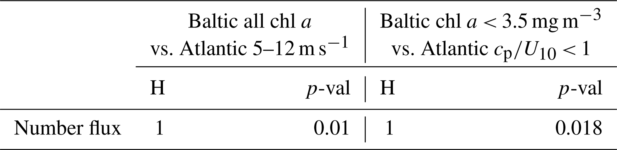
In the case of aerosol number fluxes, the results of statistical testing showed no difference between the Baltic fluxes measured at low chl a concentrations and the Atlantic fluxes. However, the right-sided Welch test showed that aerosol fluxes for the entire chl a concentration range have significantly higher values than fluxes measured in the Atlantic. This result is due to the observed increased Baltic aerosol emission in the 8–10 m s⁻¹ range for higher chl a concentrations visible in Fig. 2. As shown in Sect. 4.1.1, with further increase in wind speed, a statistically significant damping of Baltic aerosol emissions is observed compared to emissions measured at low chl a values. Due to the lack of observations of aerosol emission in the Atlantic region at wind speeds greater than 12 m s⁻¹, the further evaluation of the phenomenon is not possible. In the case of volume fluxes, all tests showed no significant differences in the values of both datasets.

Based on our analysis, we speculate that the biological activity of seawater represented by chl a significantly contributes to the differences in SSA emissions. The observed lack of difference between volume fluxes suggests that this process mainly concerns smaller submicron particles, which dominate the aerosol number flux. This may be related to the reproducible result from several studies that show that organic compounds contribute insignificantly to the supermicrometer SSA but that, in the submicrometer, the organic sea spray fraction increases with decreasing diameter until it approaches 80 % around 0.1 µm D_p (see references in the Introduction).

Another difference in emissions was observed when considering the influence of wave field properties. In order to compare statistically, we separated the datasets measured for “young” waves ($c_{\mathrm{p}}/U_{\mathrm{10}}$ < 1) and “old” waves ($c_{\mathrm{p}}/U_{\mathrm{10}}$ > 1). The results showed that the emissions from the Baltic Sea for young waves are statistically significantly higher than the emissions from the Atlantic Ocean. In the case of old waves, the Welch test showed no statistically significant differences in aerosol emissions between the Atlantic Ocean and the Baltic Sea.

4 Summary and conclusions

In this study, we present results of multi-year gradient measurements of aerosol fluxes in the Baltic Sea and the North Atlantic Ocean from a research vessel. The amount of data collected allowed us to investigate the influence of a wide range of sea- and atmosphere-related parameters and size distribution SSA fluxes in the range of 0.5 to 47 µm. We observed a statistically significant suppressing effect of marine biological matter represented by chl a concentration on SSA fluxes. The threshold chl a concentration value above which we observed the suppressing effect was 3.5 mg m⁻³. Further parameterizations were performed for fluxes measured at chl a concentrations below this value in order to keep them comparable between the Baltic and Atlantic waters. We observed high and statistically significant correlations of SSA emissions with the following parameters: wind speed, wind acceleration, wave age, significant wave height, and wave Reynolds number.

In addition, for seawater and air temperature, we observed a negative correlation with temperatures for the concentration flux and a positive correlation with temperatures for the volume flux. The values of both correlations and the presented parameterizations were statistically weak.

The main factors that we identified that influence the differences between the Baltic Sea and the Atlantic Ocean are the presence of chl a and the properties of the wave field. Statistical analysis showed that elevated chl a concentrations were associated with suppression of emissions at higher wind speeds (above 10 m s⁻¹) in the Baltic Sea. We also found no statistically significant differences between the Baltic Sea and the North Atlantic at low chl a concentrations. In the case of the wave field properties represented by the wave age parameter, we showed that aerosol emissions from the Baltic Sea were statistically significantly higher for “young” waves than from the Atlantic Ocean.

The parameterizations we developed were compared with other aerosol source functions. Our measured fluxes – both total fluxes and size distributions – as a function of wind speed are in good agreement with previous studies. Our results are in particularly good agreement with the parameterization of Kirkevåg et al. (2013). In the case of the variability in size distributions as a function of Reynolds number, the parameterization of Zinke et al. (2024) reproduces our measurements well. The Ovadnevaite et al. (2014) function, on the other hand, clearly underestimates aerosol emissions. For total fluxes dependent on the significant wave height and wave Reynolds number, the Zinke et al. (2024) function overestimates Atlantic fluxes and underestimates Baltic Sea fluxes.

Our study is the first to compare aerosol emission measurements using the same method in two different marine environments. In addition, the analysis of a large database of aerosol fluxes measured under various atmospheric and oceanographic conditions allows a broader presentation of the influence of various factors on emission. The Baltic Sea is particularly distinguishable in this respect, where the dynamics in the chemical composition of water and temperature changes are greater than in the waters of the Atlantic Ocean. This work identifies possible factors influencing the differences between these regions. A more extensive sea spray aerosol observation effort is still needed, and the contribution of water temperature, atmospheric stability, and marine biology on sea spray fluxes especially should be investigated further.

Appendix A: Flux overview

Table A1 The Baltic Sea flux overview.

Table A2 The Atlantic Ocean flux overview.

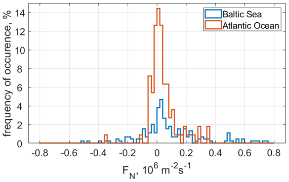
Figure A1 Flux frequency distribution after the data cleaning of measurements from the Baltic Sea (blue line) and the Atlantic Ocean (orange line).

Appendix B: CSASP-100-HV description

This section describes the classical scattering aerosol spectrometer PMS model CSASP-100-HV of Particle Measuring Systems, Inc.

The device was successfully used many times in different studies (e.g., Hoppel et al., 1994; Jensen et al., 2001; Petelski, 2005; Savelyev et al., 2014; Markuszewski et al., 2017; Bruch et al., 2023).

The CSASP uses a 5 mW He–Ne laser. The instrument samples an air volume of 12.6 cm³ s⁻¹ at a flow velocity of 32.8 m s⁻¹. The device works in four size range modes. In each mode there are 15 channels of size bins: mode 0 (diameter size range 2–47 µm with interval 3 µm), mode 1 (2–32 µm with interval 2 µm), mode 2 (1–16 µm with 1 µm), and mode 3 (0.5–8.0 µm with size interval 0.5 µm).

A photo of the device and a way of placement are presented in Fig. B1.

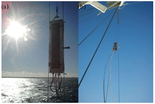
Figure B1 The classical aerosol spectrometer (left) and the method of the device moving between altitude levels during gradient measurements (right).

Appendix C: Sea spray aerosol fluxes calculated using an aerosol gradient

To evaluate the aerosol gradient flux equation, let us start with the wind gradient formula:

$$\begin{array}{}\text{(C1)}& {\displaystyle \frac{\mathrm{d}U}{\mathrm{d}z}}={\displaystyle \frac{u_{*}}{kz}},\end{array}$$

where $\mathrm{d}u/\mathrm{d}z$ is the wind speed profile of the function of altitude z and u_* is the friction velocity defined from the definition of the momentum flux τ as

$$\begin{array}{}\text{(C2)}& \mathit{\tau }\equiv \mathit{\rho }{u}_{*}^{\mathrm{2}},\end{array}$$

where ρ is the fluid density.

The general solution of Eq. (C1) is given by Panofsky (1963):

$$\begin{array}{}\text{(C3)}& u\left(z\right)={\displaystyle \frac{u_{*}}{kz}}[\ln \left(z/z_{\mathrm{0}}\right)-{\mathit{\psi }}_m\left(z/L\right)],\end{array}$$

where z₀ is the roughness length for the wind profile, ψ_m is the diabatic correction to the logarithmic wind profile in Monin–Obukhov theory, and L is the Monin–Obukhov length.

A similar approach is used for other scalars, such as the potential temperature profile. Therefore, it is also possible to apply it for the aerosol concentration (N) profile:

$$\begin{array}{}\text{(C4)}& {\displaystyle \frac{\mathrm{d}N(z,D_{\mathrm{p}})}{\mathrm{d}{D}_{\mathrm{p}}}}={\displaystyle \frac{\mathrm{d}{N}_{*}\left(D_{\mathrm{p}}\right)}{\mathrm{d}{D}_{\mathrm{p}}}}\ln \left(z\right)+C\left(D_{\mathrm{p}}\right),\end{array}$$

where N_* represents the aerosol concentration gradient analogues of u_*.

Using the least-squares method, where N_* is the linear coefficient of approximation and C is the free coefficient, the correlation coefficients r of each linear fitting were calculated within aerosol concentration gradient calculations. Results with correlations less than 0.4 were excluded from further analysis.

By differentiating the above equation, we obtain

$$\begin{array}{}\text{(C5)}& {\displaystyle \frac{d}{\mathrm{d}z}}\left({\displaystyle \frac{\mathrm{d}N\left(D_{\mathrm{p}}\right)}{\mathrm{d}{D}_{\mathrm{p}}}}\right)={\displaystyle \frac{\mathrm{1}}{z}}{\displaystyle \frac{\mathrm{d}{N}_{*}\left(D_{\mathrm{p}}\right)}{\mathrm{d}{D}_{\mathrm{p}}}}.\end{array}$$

Let us multiply both sides with the momentum diffusivity coefficient with the assumption of near-neutral stratification ($K_h=kz{u}_{*}$) and treat aerosol concentration as a scalar. Based on that, we can define aerosol flux:

$$\begin{array}{}\text{(C6)}& -u_{*}kz{\displaystyle \frac{d}{\mathrm{d}z}}\left[{\displaystyle \frac{\mathrm{d}N\left(D_{\mathrm{p}}\right)}{\mathrm{d}{D}_{\mathrm{p}}}}\right]=-k{u}_{*}{\displaystyle \frac{\mathrm{d}{N}_{*}\left(D_{\mathrm{p}}\right)}{\mathrm{d}{D}_{\mathrm{p}}}}\equiv {\displaystyle \frac{\mathrm{d}{F}_N\left(D_{\mathrm{p}}\right)}{\mathrm{d}{D}_{\mathrm{p}}}}.\end{array}$$

Using this formula, it is possible to determine aerosol vertical flux in near-neutral stratification of the marine boundary layer. Detailed considerations about the determinations of the above formulas are given by Panofsky (1963), Petelski (2003), and Andreas (2007).

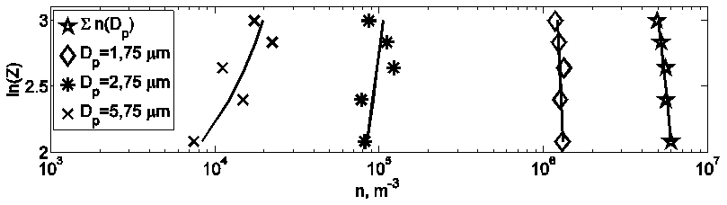
Figure C1 Exemplary linear fitting to vertical profiles of aerosol concentration for exemplary size bins. Measurement carried out during the Baltic cruise, 21 February 2013.

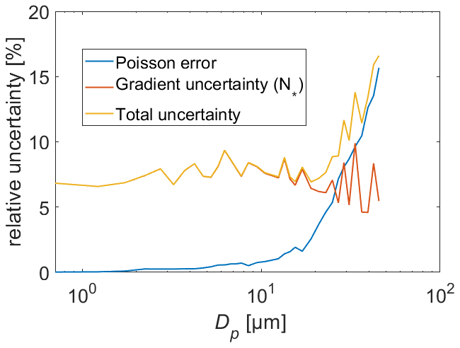
Figure C2 Relation of measurement uncertainties with aerosol size distribution measured with the CSASP.

The obtained aerosol concentration scale N_* multiplied by u_* gives the aerosol concentration flux according to Eq. (C6). u_* was calculated using our wind speed measurements using the formula given by Large and Yeager (2004). This methodology was applied for total aerosol concentration and for each of 36 size bins.

Obtained fluxes were corrected for dry deposition flux and calculated in each size bin using deposition velocity proposed by Schack Jr. et al. (1985).

In the end, all fluxes were also reduced to 80 % equilibrium humidity using the Fitzgerald (1975) formula updated with the recent sea spray growth factor given by Zieger et al. (2017). In this paper, all aerosol and flux spectra are presented in relation to reduced diameters, which were marked later as D_p@80 % (diameter at 80 % humidity).

Exemplary results of such fitting are presented in Fig. C1.

As we can see in Fig. C2, the Poisson error up to 16 µm is low (below 2 %), with a very small increase with size distribution. For a higher particle size range, the error increases up to 16 % for the last aerosol channel. The uncertainty of the gradient method oscillates around a constant value of 7 %. The total uncertainty of flux measurement is the sum of these two elements.

Appendix D: Statistical test results

In order to proceed with the statistical comparisons, we first need to run Levene's test (Levene, 1960), which is an inferential statistic used to assess the equality of variances for a variable calculated for two or more groups. Testing proved that there was a statistically significant difference between all analyzed pairs of data. After proving the variance difference, it is possible to run Welch's t test, (or unequal variances t test; Welch, 1947), a two-sample location test which is used to test the (null) hypothesis that two populations have equal means.

Table D1 The Welch t test results between source functions fitted to Baltic Sea fluxes. $P_{\mathrm{B}}^{\mathit{\alpha }}(U_{\mathrm{10}}$) represents the function fitted to all data, and $P_{\mathrm{B}}^{\mathit{\beta }}(U_{\mathrm{10}}$) is the function fitted to low chl a cases only. The left side of the table shows the test result for mean difference between the functions. On the right side of the table, the right-tailed Welch t test results shows that, for wind speed above 10 m s⁻¹, the function $P_{\mathrm{B}}^{\mathit{\alpha }}(U_{\mathrm{10}}$) is significantly higher than the function with the low chl a case.

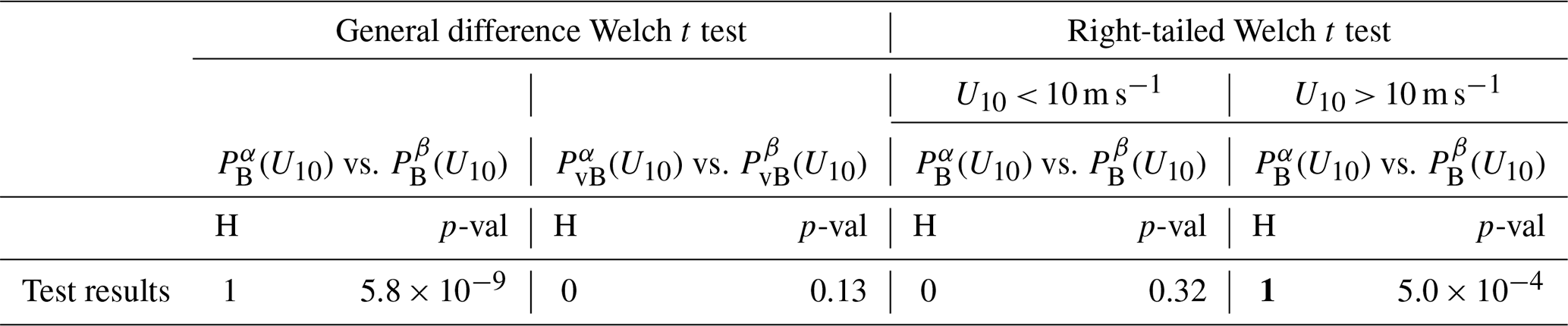
Table D2 Welch t test results of total fluxes measured in the Baltic Sea region compared with fluxes measured in the Atlantic Ocean area. Fluxes were compared for the same wind speed ranges of 5–12 m s⁻¹ (first two columns) and two cases of wave ages: young $c_{\mathrm{p}}/U_{\mathrm{10}}$ < 1 and old $c_{\mathrm{p}}/U_{\mathrm{10}}$ > 1 (third and fourth columns).

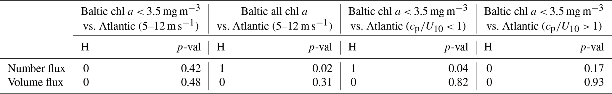
Table D3 Right-tailed Welch t test results of comparison between Baltic and Atlantic total fluxes in the same wind speed range (first column) and for young waves only (second column).