the Creative Commons Attribution 4.0 License.
the Creative Commons Attribution 4.0 License.
 | 05 Jan 2024
Climatologically invariant scale invariance seen in distributions of cloud horizontal sizes
Thomas D. DeWitt
Karlie N. Rees
Corey Bois
Steven K. Krueger
Nicolas Ferlay
Cloud area distributions are a defining feature of Earth's radiative exchanges with outer space. Cloud perimeter distributions n(p) are also interesting because the shared interface between clouds and clear sky determines exchanges of buoyant energy and air. Here, we test using detailed model output and a wide range of satellite datasets a first-principles prediction that perimeter distributions follow a scale-invariant power law n(p) ∝ , where the exponent β = 1 is evaluated for perimeters within moist isentropic atmospheric layers. In model analyses, the value of β is closely reproduced. In satellite data, β is remarkably robust to latitude, season, and land–ocean contrasts, which suggests that, at least statistically speaking, cloud perimeter distributions are determined more by atmospheric stability than Coriolis forces, surface temperature, or contrasts in aerosol loading between continental and marine environments. However, the satellite-measured value of β is found to be 1.26 ± 0.06 rather than β = 1. The reason for the discrepancy is unclear, but comparison with a model reproduction of the satellite perspective suggests that it may owe to cloud overlap. Satellite observations also show that scale invariance governs cloud areas for a range at least as large as ∼ 3 to ∼ 3 × 10⁵ km2, and notably with a corresponding power law exponent close to unity. Many prior studies observed a much smaller range for power law behavior, and we argue this difference is due to inappropriate treatments of the statistics of clouds that are truncated by the edge of the measurement domain.
- Article
(2428 KB) - Full-text XML
-
Supplement
(604 KB) - BibTeX
- EndNote


Since the first numerical global climate models (GCMs) were developed in the 1960s, there have been exponential advances in computational capabilities that have led to spectacular simulations of cloud structures. The next generation of climate models is expected to resolve individual clouds at kilometer scales (Schär et al., 2020). The strategy behind this “bottom-up” approach to representing the role of clouds in climate is that pursuing ever finer spatial resolution and improved model physics will lead to more accurate predictions, accepting the necessary evil of increased computational expense (Slingo et al., 2022). Yet, perhaps alarmingly, it has not been clear that this approach has been successful in its goal given that the spread in GCM predictions of the climate sensitivity to greenhouse gases has, if anything, only increased (Palmer, 2016; Arias et al., 2021; Lovejoy, 2022).
In some sense, time-dependent deterministic simulations are not obviously well suited for obtaining a statistical time-independent climatology. An alternative approach might be to derive the statistics directly, using principles of statistical thermodynamics, from bulk physical constraints (Arakawa, 2004; Procyk et al., 2022). A familiar example is the simplicity of the derivation of the Maxwell–Boltzmann statistics characterizing the distribution of speeds of molecules in an ideal gas, obtained knowing only the average energy per molecule and without deterministically simulating individual particles and the extraordinary complexities of their quantum mechanical interactions (Schroeder, 2021). There is some evidence that this “top-down” philosophy may work for convective cloud fields. An exponential distribution of mass fluxes can be derived for non-interacting clouds by considering only the large-scale vertical mass flux (Cohen and Craig, 2006; Craig and Cohen, 2006). Another study by Garrett et al. (2018) took a similar top-down approach but allowed for cloud interactions. It obtained a distribution of cloud horizontal sizes in a steady state that follows an exponential in saturated static energy and a power law with respect to cloud perimeter.
In this study, we use a range of satellite observations to test the validity of the cloud perimeter distribution derived by Garrett et al. (2018). We show that both cloud perimeters and cloud areas do indeed follow a power law but that the power law exponent appears to be a function of perspective, agreeing well with theory in thin horizontal layers in cloud-resolving models but not with satellite observations of cloud fields looking down from space. We also find that the choice of domain size and treatment of clouds that are truncated by the domain edge can introduce spurious scale breaks in power law size distributions. We suggest that previous results that do not account for these subtle effects should be interpreted with caution.
This paper is organized as follows. In Sect. 2, we first provide an overview of the theoretical arguments presented by Garrett et al. (2018) that led to the predicted cloud perimeter distribution. With this necessary background, prior empirical measurements of the related cloud area distribution are then discussed, along with the subtleties involved in measuring distributions of cloud sizes. The methods are presented in Sect. 3, and results from satellite observations are presented in Sect. 4. In Sect. 5, we examine the role of perspective in measuring cloud size distributions and finally conclude in Sect. 6.
To begin, we justify why it is physically meaningful to look at cloud perimeters by summarizing the derivation of the cloud perimeter number distribution n(p) presented by Garrett et al. (2018). The foundation follows a parcel through an idealized thermodynamic cycle around cloud edges – what was termed a “mixing engine” – defined by four “legs”:
-
moist adiabatic ascent inside cloud
-
diabatic mixing with clear air across cloud edge that dries the parcel and reduces cloud perimeter
-
dry adiabatic clear-sky descent
-
diabatic mixing with cloudy air across cloud edge that moistens the parcel and lengthens cloud perimeter.
The cycle is analogous to the familiar Carnot cycle, used to describe hurricanes (Emanuel, 1991), but with entropy generation associated with mixing at the cloud edge rather than with energetic exchanges with the oceans or outer space. In observations of tropical convection, Heus and Jonker (2008) found that shallow cumulus clouds tend to have a neutrally buoyant cloud edge and a “subsiding shell” of descending clear air adjacent to the cloud edge. A similar pattern was later observed in local circulations around simulated deep convection (Glenn and Krueger, 2014). These observations appear to support the mixing engine framework, at least for actively convecting clouds.
Representing mass fluxes across cloud edges in 4D space-time coordinates, as is typically done in detailed cloud numerical simulations, is difficult because turbulent mixing changes both the location and length of the cloud edge itself and over a very wide range of time and space scales. However, while the cloud edge may deform during mixing, it maintains its position as a point of approximate neutral buoyancy and in this sense can serve as a fixed reference point in a related coordinate system. For this purpose, we use the moist static energy, which is given by
where g, cp, and Lv are the gravitational acceleration, the specific heat of air at constant pressure, and the latent heat of vaporization of water, respectively, and z, T, and q are height, temperature, and the water vapor mixing ratio, respectively. At the cloud edge, air is just saturated, so the moist static energy is equal to the saturated static energy, defined as , where q⋆ is the saturated mixing ratio. At a given height, perturbations in saturated static energy can be related to temperature (and hence buoyancy) perturbations T′ through , where (Randall, 1980).
In a tropical atmosphere, variability in h⋆ between horizontal levels dominates variability within a given level, so a constant h⋆ surface can be approximated as lying along a surface of constant z (Xu and Emanuel, 1989). Supposing a thin atmospheric layer of thickness δz, clouds within this layer can be partitioned into discrete bins j of mean perimeter pj. For a number nj of such clouds, each bin has a total cloud perimeter njpj and a total surface area σ=njpjδz. This surface area is the component of the overall cloud surface area that is vertically oriented. Fick's law suggests that for bin j, the total rate of dissipation of potential energy across the cloud edge Qj due to diabatic turbulent mixing is proportional to the product of the energy gradient between cloudy and clear air ∇h and the total surface area σ (Garrett, 2012; Garrett et al., 2018). Provided that the perturbation from the domain mean δh is much smaller than the mean value 〈h⋆〉, a constraint that is satisfied even over the entire depth of the troposphere, and that turbulence around cloud edges is approximately isotropic (Heus and Jonker, 2008; Heus et al., 2009; Wang et al., 2009), the vertical and horizontal legs of the mixing engine are approximately the same size, so δx≈δz and , where S is the stability. Thus the rate of dissipation of energy due to horizontal mixing across the cloud edge in any given size bin j is
In any cloud field, clouds continually grow and shrink due to turbulent mixing processes, and so cloud number is passed from one perimeter bin j to the next j+1 or j−1. In a steady state, however, which can be defined as a time-invariant perimeter distribution, there must be no net convergence of cloud number or energy into any bin j. This implies that or in discretized form from Eq. (2) that njpj=const. The steady-state perimeter distribution n(p) can therefore be expected to follow the power law (Garrett et al., 2018)
Power laws such as Eq. (3) are generally considered to be “scaling”, since a rescaling of p by some constant factor c results in a constant rescaling of n(p) by a constant factor . Of course, it is impossible for any physical system to exhibit scale invariance over an infinite range of scales, and so such scaling behavior can only be valid over a finite range . Beyond these “scale breaks”, the value of β changes, or the functional form of the distribution changes. As an example, a common feature of power law distributions describing many other natural and social systems is an exponential cutoff at large scales (Newman, 2005; Clauset et al., 2009).
For clouds, as a guess, the smallest possible size defining pmin might be the Kolmogorov microscale for turbulent circulations such as in the mixing engine, whose order of magnitude is ∼1 mm (Tennekes and Lumley, 1972). The largest possible clouds are of course limited by the Earth's circumference of ∼105 km but might be more reasonably constrained by the Rossby radius of deformation ∼103 km where Coriolis forces limit horizontal spreading.
Since cloud edges are fractal (Lovejoy, 1982), calculated perimeter lengths depend on the chosen measurement resolution, so pmax can be orders of magnitude larger than the distance from one end of a cloud to the other. A measure of maximum cloud size that is less resolution-dependent is maximum cloud area, which is roughly 𝒪(cloud length)2.
The continuous function n(p) can be discretized into linearly spaced bins with constant Δp, in which case the slope on a plot with two logarithmic axes would be . If logarithmically binned with constant Δln p, the slope of the power law would be −β because . We favor logarithmically spaced bins as being better suited to describe the vast range of cloud sizes because linearly spaced bins increase sampling uncertainty in large bins with few counts (White et al., 2008).
The challenge of measuring cloud size distributions
For the power law exponent β, Garrett et al. (2018) found in a comparison with a highly detailed numerical simulation of a tropical cloud field, in close agreement with the theoretically expected value of β=1. Cloud perimeter distributions have yet to be assessed observationally, although cloud area distributions have been widely studied, generally revealing power law distributions in both satellite observations (Cahalan and Joseph, 1989; Kuo et al., 1993; Benner and Curry, 1998; Koren et al., 2008; Wood and Field, 2011) and models (Neggers et al., 2003; Yamaguchi and Feingold, 2013; Neggers et al., 2019; Christensen and Driver, 2021), although not in every study (López, 1977). Assuming both cloud areas and perimeters are power-law-distributed, the two quantities can be related by the scaling relationship
D is often interpreted to be the fractal dimension Df as it is formally defined by the relation relating how the measured length l of a fractal line such as cloud perimeter depends on the “ruler length” (or resolution) ξ used to measure it (Mandelbrot, 1982). Assuming the relationship D=Df is valid, the fractal dimension can be determined by fitting a linear regression between observations of and ln p (e.g., Lovejoy, 1982; Cahalan and Joseph, 1989; Siebesma and Jonker, 2000; Christensen and Driver, 2021).
Subsequent work has shown that, for clouds, D is not in fact strictly equivalent to the fractal dimension Df. Batista-Tomás et al. (2016) and Peters et al. (2009) pointed out that adopting the equivalence D=Df requires holes in clouds to be excluded from contributing to the cloud's perimeter, as the fractal dimension is a property of a single curve (a cloud's exterior perimeter) rather than an ensemble of curves (a cloud's exterior perimeter and the perimeter of each hole).
Furthermore, Imre (1992) showed that the constant pre-factor in Eq. (4) often itself scales with a. In this case, fitting a regression line to a scatterplot of vs. ln p would yield a value for D that implicitly includes a scaling contribution from the supposed “constant”.
Setting aside these details, a scaling of the form Eq. (4) nonetheless can be used to empirically relate cloud areas and perimeters, making the expression useful regardless of any particular interpretation of D. Here, it permits the perimeter size distribution Eq. (3) to be converted to a distribution in cloud area. Since dln a∝dln p, , and so
Adopting (Lovejoy, 1982; Siebesma and Jonker, 2000), noting that both higher (Cahalan and Joseph, 1989; Christensen and Driver, 2021) and lower (Cahalan and Joseph, 1989; Batista-Tomás et al., 2016) values have been measured, and β=1 as proposed by Garrett et al. (2018), Eq. (5) yields . By contrast, widely conflicting values are observed for α, as well as for the location of the scale break amax. Cahalan and Joseph (1989) and Benner and Curry (1998) found in satellite observations values for amax ranging from 4 km2 to between 0.28 and 0.62 km2, respectively. In large-eddy simulations, Neggers et al. (2003) found scale breaks between km2.
For larger domains considered in other studies amax tends to be larger. Wood and Field (2011) found using MODIS satellite data that and amax≳106 km2. Peters et al. (2009) found a scale break in mesoscale convective clusters at amax∼105 km2, although it depended on the value of a threshold based on column water vapor. Conversely, Christensen and Driver (2021) found amax∼106 km2 for tropical deep convection. There is also variation in calculated values for α, with Koren et al. (2008) finding and Yamaguchi and Feingold (2013) finding α=0.59. Neither found evidence for a scale break amax, although they considered smaller domains.
These conflicting results could reflect meteorological differences, as there is some evidence that D, or α through Eq. (5), is itself dependent on cloud type and size (Cahalan and Joseph, 1989; Batista-Tomás et al., 2016). However, a largely overlooked explanation for the surprising variance in values for α and amax is one of sampling bias. Larger clouds are more likely to be truncated by the edge of the measurement domain than small clouds, and if they are removed from the analysis, as is sometimes done, there can be a spurious scale break introduced to the size distribution. Such a scale break would depend only on the size of domain considered, rather than some intrinsic physical property of the cloud field itself. This spurious effect of domain size has also been found to influence the measured power law exponent for idealized 1D cloud sizes (Wood and Field, 2011).
Past studies generally do not mention how clouds truncated by the domain edge are treated, or, in some cases, they simply remove them from analysis (e.g., Peters et al., 2009; Christensen and Driver, 2021). Plausibly, some of the inconsistencies seen in measured values of amax and α could owe to this measurement problem. For example, one seeming solution is to retain clouds that are truncated by the domain edge but measure only the portion of the cloud area that lies within the domain. With this approach, a portion of the given cloud's area is necessarily omitted, likely placing it in a smaller size bin where counts are consequently oversampled.
Our goal here is to test in satellite observations and models the hypotheses proposed by Garrett et al. (2018), namely that β=1 as specified by Eq. (3) and that the value of β is the same for any cloud field in a steady state. Second, we attempt to address inconsistencies in previous observations of α and amax by appropriately accounting for bias introduced by the treatment of clouds truncated by the edge of a satellite measurement domain.
3.1 Satellite datasets
The satellite platforms used to image clouds in this study fall into two broad categories: full disk and polar-orbiting. Full-disk images are effectively a snapshot of Earth taken from geostationary orbit or, in the case of EPIC, the L1 Lagrange point. Polar-orbiting sensors continuously scan a rectangular swath as they move poleward. Details about the datasets are summarized in Table 1.
Derrien and Gléau (2005, 2010)Derrien and Gléau (2005, 2010)Derrien and Gléau (2005, 2010)Derrien and Gléau (2005, 2010)Derrien and Gléau (2005, 2010)Yang et al. (2019)Kopp et al. (2014)Ackerman et al.19982008Buriez et al.1997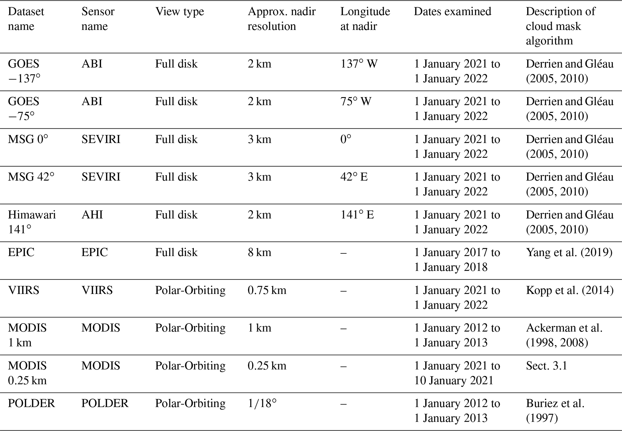
For most of the satellite datasets described in Table 1, individual clouds are identified from pre-processed binary cloud masks designed to distinguish cloudy and clear sky. The definition of a cloud is somewhat subjective, and so inevitable differences in cloud identification algorithms and sensor capabilities lead to variations in global cloud coverage estimates between datasets. Even for a given satellite dataset, estimates of global cloud fraction depend on the choice of viewing angle, increasing with more oblique perspectives (Maddux et al., 2010). To mitigate this concern, images are truncated to exclude cloud imagery where the sensor zenith angle is greater than 60∘, a choice intended as a compromise between limiting sensitivity to viewing angle while retaining a large domain area.
To test the sensitivity of measured distributions of cloud sizes to cloud definition, we also use a simple cloud mask based on MODIS band 1 optical reflectance R, which is sensitive to wavelengths between 620 and 670 nm and has a resolution at nadir of 0.25 km. We examine 13 tropical maritime granules, each centered between approximately 10∘ S and 20∘ N and 115∘ W and 140∘ W and covering an area approximately 1950 km wide by 2030 km long. Images from each granule were visually inspected for artifacts from sun glint, and several additional granules were omitted from the analysis due to sun glint contamination. Figure 1 compares several example cloud masks generated using various thresholds in R alongside the pre-processed cloud mask and an RGB image.
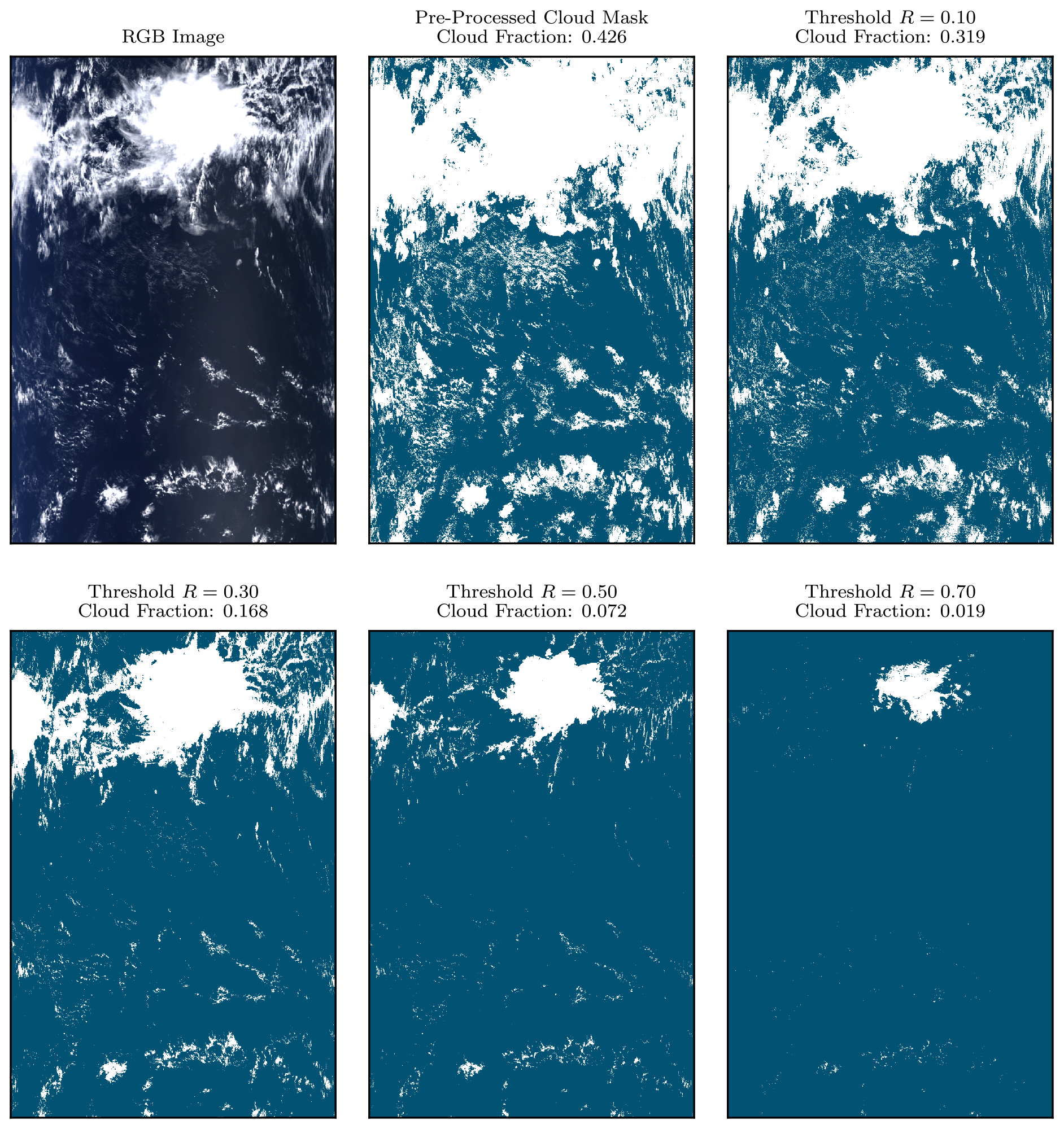
Figure 1Example RGB image, pre-processed cloud mask, and cloud masks created from various thresholds in optical reflectance R for a single MODIS granule. In the reflectance-based cloud masks, pixels with reflectance higher than the threshold are set to cloudy (white), while the others are set to clear (dark blue). The image is centered at approximately 1∘ S, 130∘ W and was taken on 1 January 2021 at approximately 19:05 UTC. Note that pixels are depicted here as being uniform in size but that cloud size calculations account for pixel size increasing away from nadir.
3.2 SAM numerical simulations
For numerical simulations of cloud fields, we use output from the System for Atmospheric Modeling (SAM) (Khairoutdinov and Randall, 2003). SAM was initialized and forced by large-scale thermodynamic tendencies derived from mean conditions during the GATE Phase III field experiment (Khairoutdinov et al., 2009) and run with prescribed radiative heating and diagnostic subgrid-scale turbulence. From two prognostic hydrometeor variables (precipitating and non-precipitating), cloud water, cloud ice, rain, snow, and graupel are diagnosed. The simulation's domain size is 204.8 km × 204.8 km with 100 m horizontal grid spacing and a 2 s time step. The vertical grid spacing is 50 m below z=1.2 km and increases to 100 m at z=5 km. There are a total of 210 vertical levels.
Shallow cumulus form in the first hour of the simulation, gradually deepening into deep convection by hour 6. Beyond approximately hour 12, a steady-state period is reached where the convection is in quasi-equilibrium with the prescribed large-scale forcing (Arakawa and Schubert, 1974; Lord and Arakawa, 1980; Lord, 1982). During this steady-state period, the precipitation rate and cloud cover fluctuate without significant trends, and the simulation does not self-aggregate (Khairoutdinov et al., 2009). We analyze hourly 3D model output from hours 12 to 24. Output from this simulation was also used in Garrett et al. (2018) and is described in full detail in Khairoutdinov et al. (2009).
A cloud mask for each horizontal layer in the simulation was applied by setting all grid cells with non-precipitating cloud condensate mixing ratios qn (including both liquid and ice) in excess of 1 % of the saturated mixing ratio q⋆ to cloudy and the remainder to clear. Once every grid cell is defined as either cloudy or clear, 2D images were created by isolating each individual height level in the domain, creating 210 images for every time step. These images were then analyzed separately using the same method as the satellite imagery (described below). Isolating individual horizontal layers in this manner provides an approximate method of isolating constant h⋆ surfaces (Garrett et al., 2018). After perimeters were calculated and binned for each layer, counts were summed over all layers. We also create a “satellite-like” image from the simulation, which is described in Sect. 5.
3.3 Cloud identification and filtering
Both the satellite and model datasets yield 2D binary cloud masks where grid cells or pixels are either cloudy or clear. Individual clouds are defined as connected cloudy regions, identified by applying a convention that adjacent cloudy pixels are connected, whereas diagonal cloudy pixels are not (termed “4-connectivity”; Wood and Field, 2011; Christensen and Driver, 2021), although the analysis is not significantly affected by this choice (Kuo et al., 1993). In the satellite datasets, the pixel lengths in the x and y directions are determined independently as a function of satellite distance and sensor zenith angle.
The cloud perimeter is then computed by summing all pixel side lengths along the edge of the cloud and cloud area by summing the areas of each individual cloudy pixel. Cloud holes add to the cloud's perimeter but reduce its area, which as described above implies D≠Df in Eq. (4). Clouds consisting of a small number of pixels are more Euclidean than fractal (Christensen and Driver, 2021), which leads to an inaccurate estimate of the small portion of the size distribution. We therefore truncate number distributions to exclude cloud perimeters ≤ 10 × (resolution at nadir) or areas ≤ 10 × (resolution at nadir)2.
Unexpectedly the smaller portion of the size distributions obtained using EPIC display non-power-law behavior, in contrast to all other satellite datasets over similar scales. To ensure values for α and β were calculated over only the power law regime, thresholds used for EPIC clouds were increased to exclude perimeters ≤ 30 × (nadir resolution) or areas ≤ 1000 × (nadir resolution)2. Conceivably, the discrepancy is caused by a compression algorithm that averages 2×2 pixel regions before data transmission. The regions are subsequently interpolated back to the original resolution, which may smooth cloud perimeters (see Appendix A for further discussion).
To account for possible scale breaks in size distributions introduced by clouds truncated by the edge of the measurement domain, area or perimeter bins in which the number of clouds truncated by the edge is greater than 50 % of the total in that bin are removed from consideration. For the observed cloud fields, such bins tend to be those in the larger end of the size spectrum as large clouds are most likely to touch the domain edge. The threshold choice of 50 % represents a compromise, removing bins most sensitive to truncation effects while allowing for a large range of cloud sizes to be studied. Calculated values for α and β are relatively insensitive to more stringent thresholds less than 50 %.
We calculate the power law exponents α and β by performing a linear regression in logarithmic space since from Eqs. (3) and (5) and . It has been argued this method can lead to underestimates of the exponent (Clauset et al., 2009), but there is no straightforward alternative when presented, as is the case here, with a power law that has both an upper and lower bound (Hanel et al., 2017). We evaluate uncertainties as 95 % confidence intervals corresponding to 2 standard errors of the regression. We report numerical values of plotted data in the Supplement.
In satellite observations examined here, both cloud areas and perimeters are well described by a power law distribution. For cloud areas, Fig. 2 shows measured values of α ranging between (POLDER and MODIS 0.25 km) and (GOES −75∘ and Himawari 141∘) and a mean value, across all satellite datasets, of . These values are largely in agreement with several previous studies (e.g., Cahalan and Joseph, 1989, Benner and Curry, 1998, and Wood and Field, 2011).
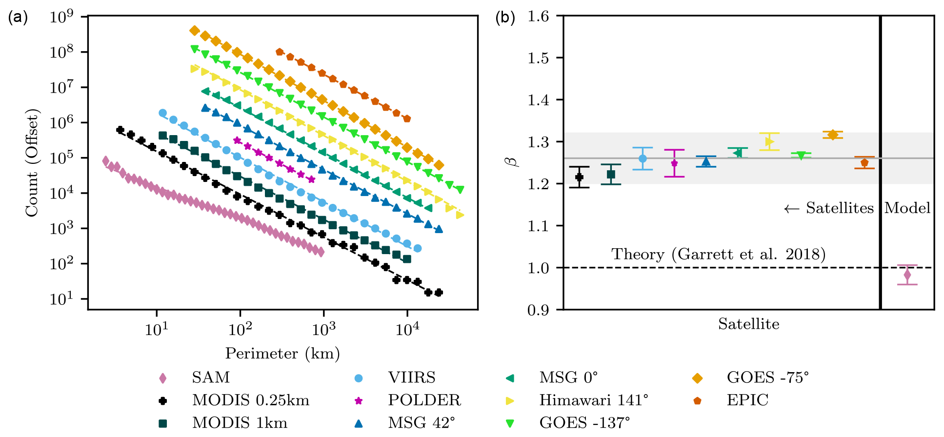
For cloud perimeters, Fig. 3 shows values of β ranging from (MODIS 1 and 0.25 km) to (GOES −75∘), with a mean across all satellite datasets of . This value differs from that found in SAM horizontal levels, where , and from the theoretically derived value of β=1 (Eq. 3).
These mean values of α and β imply, from Eq. (4), that , which is in good agreement with prior studies that have generally found values of D slightly greater than , e.g., D=1.35 (Lovejoy, 1982), (Cahalan and Joseph, 1989), or D=1.4 (Christensen and Driver, 2021).
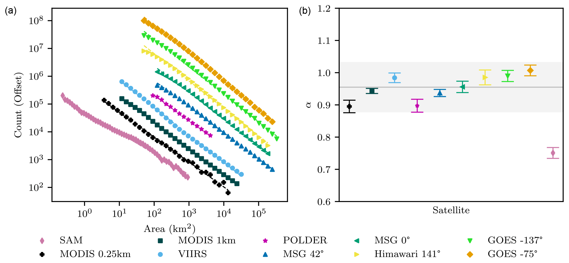
Figure 2(a) Logarithmically binned histograms of cloud areas for satellite datasets. (b) Measured values of the power law exponent α (Eq. 5) with associated mean (gray line) and 95 % confidence interval (gray box). Counts have been vertically offset for clarity. Uncertainties represent 95 % confidence intervals, derived from a linear regression standard error analysis.
After omitting bins containing 50 % or more clouds truncated by the domain edge, a scale break amax is no longer evident in the area distributions. In several cases, the distributions exhibit scale invariance extending to areas larger than 105 km2, with the largest to at least km2 (EPIC). We find that amax must therefore have a value larger than roughly 3×10⁵ km2, corresponding to an effective diameter of ∼600 km, substantially larger than some have previously suggested (e.g., Cahalan and Joseph, 1989; Benner and Curry, 1998; Neggers et al., 2003), with Wood and Field (2011) extending amax to 106 km2.
Variability with seasonality, latitude, and surface type
The perimeter size distribution, given by Eq. (3), was derived without explicit consideration of local climatological characteristics such as season, surface type, or latitudinal location (Garrett et al., 2018). In satellite observations, the sensitivity of β to such considerations is shown in Figs. 4, 5, and 6. Comparisons between latitude bands shown in Figs. 4 and 5 are restricted to observations using the polar-orbiting satellites MODIS and VIIRS because imagery from these sensors, regardless of latitudinal location, is both similar in domain area and always centered directly below the satellite. These conditions reduce the likelihood of bias due to differing viewing geometry, and neither condition holds for the full-disk images. POLDER has been omitted from Figs. 4, 5, and 6 because, when limited to smaller domains, its smaller sample size introduces significant statistical variability.
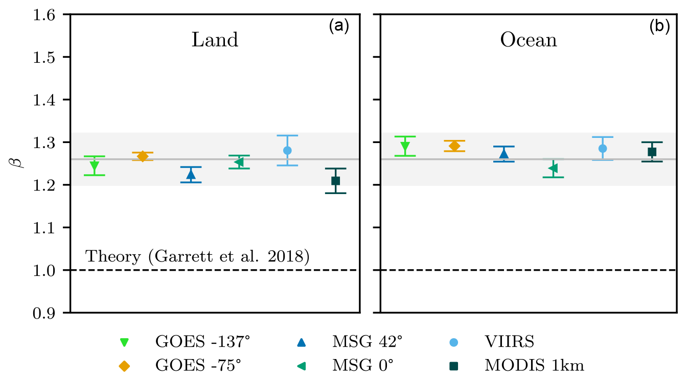
Independent of sensor, measured values of β appear robust across latitudinal regions, land–ocean contrasts, and seasons. Figure 5 does show modest variability in the value of β by month in the midlatitude regions 60–30∘ S and 30–60∘ N between a minimum value of (MODIS; March, May, June; northern midlatitudes) and a maximum value of 1.32±0.02 (MODIS; June, July; southern midlatitudes). Annual mean values of β for the midlatitude and equatorial regions in Fig. 4 show similar values ranging from for MODIS at northern midlatitudes to for VIIRS in all regions and MODIS at southern midlatitudes. Separating clouds by marine and continental regions in Fig. 6, mean values for β are 1.25±0.05 for land and 1.28±0.04 for ocean. All values are consistent with the global mean value across datasets of .
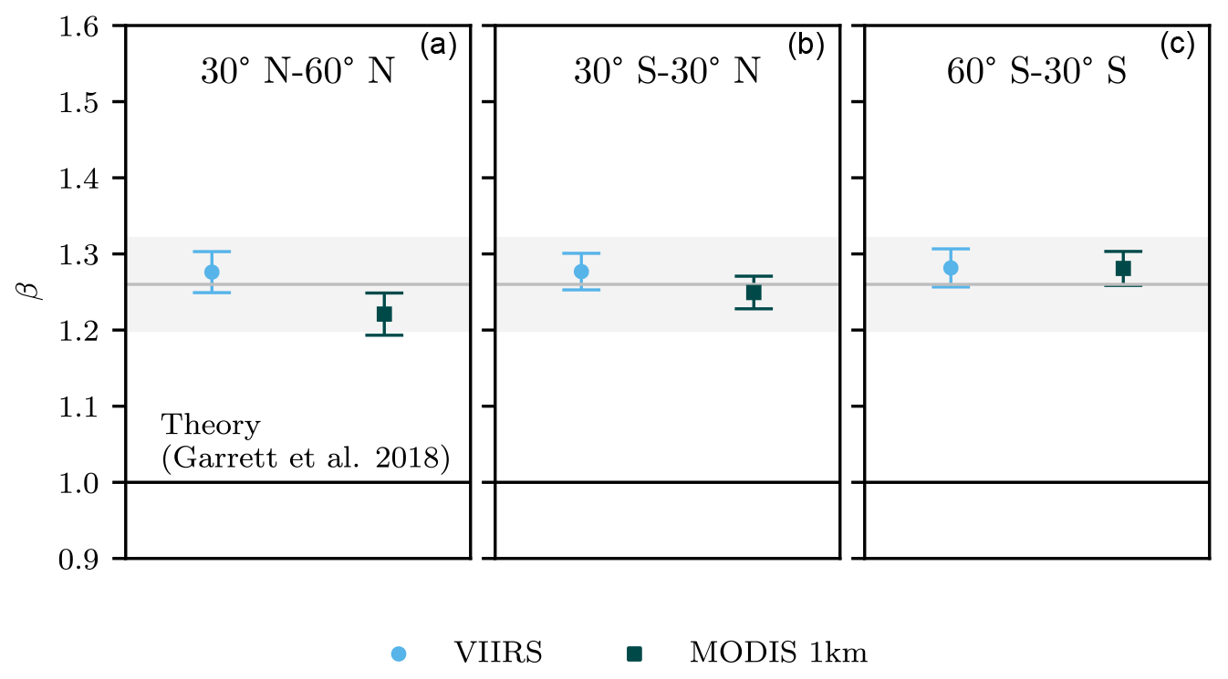
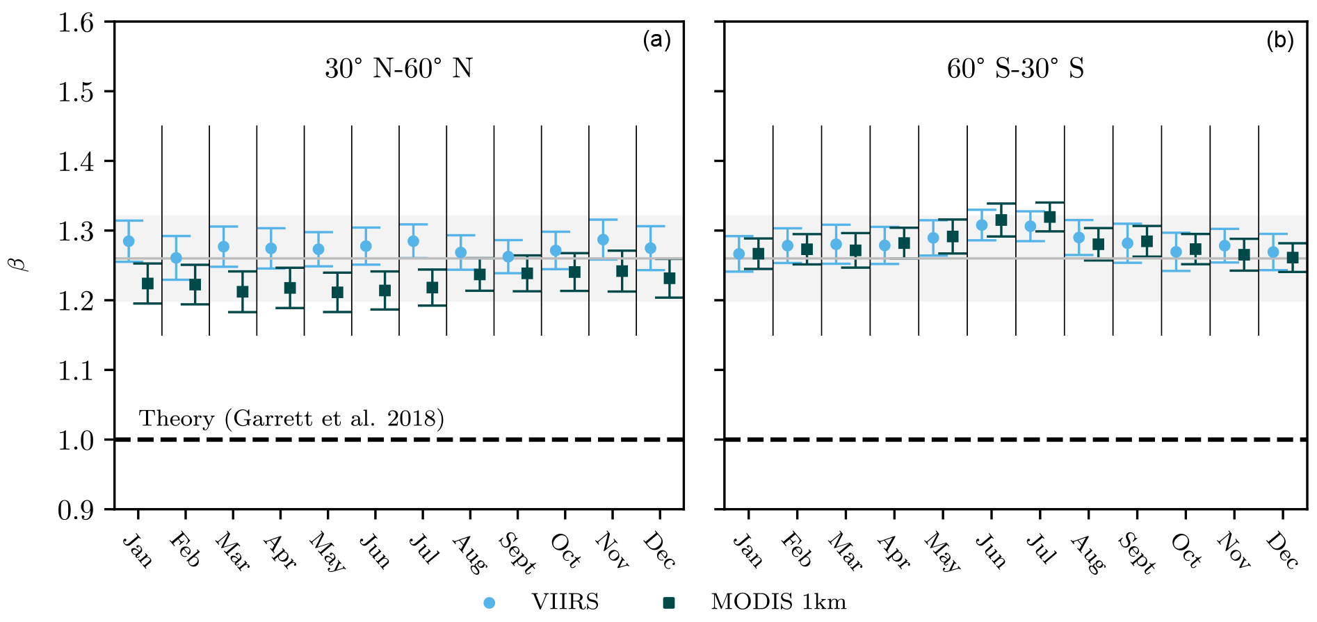
Figure 5Measured values of β (Eq. 3), for the northern midlatitude region (a) and the southern midlatitude region (b), separated by month. The equatorial region (not shown) shows similar variability around a mean value shown in Fig. 4. The gray line and box represent the global mean and 95 % confidence interval, respectively, from Fig. 3.
After accounting for spurious scale breaks introduced by the problem of attempting to measure the extent of scale invariance with a finite domain, we find that a power law describes the distributions of both cloud perimeters and areas for a size range spanning 4 and 5 orders of magnitude, respectively, and likely extends even further. This result is perhaps all the more remarkable for the fact that the value of the exponent β appears to be robust to such local climatological characteristics as season, latitude, land–ocean contrasts, and latitude, which might be related to surface temperature, the Coriolis force, dominant cloud type, or aerosol loading. In this sense, the observations appear to lend support to the general theoretical “mixing engine” approach employed by Garrett et al. (2018) to obtain Eq. (3), where β was derived only by considering mixing processes at the cloud edge.
However, a puzzle remains: the global mean value of in satellite observations is higher than the value of β≃1 obtained both theoretically (Eq. 3) and from SAM model simulations (Fig. 3). The difference is significant given the range of scales in cloud sizes involved. For example, for a roughly 3-order-of-magnitude measured range for cloud perimeters, the discrepancy would imply an order-of-magnitude difference in cloud counts.
The most obvious inference is that the theory is missing something fundamental about what determines cloud perimeters, even if it produced perimeter distribution values of β very close to those seen in a highly detailed numerical cloud model. Alternatively, one important distinction that may be made between the two approaches is simply one of perspective. Perimeter distributions from the numerical model SAM shown in Fig. 3 and previously in Garrett et al. (2018) were calculated by treating every individual horizontal layer in the SAM volume as an independent 2D image. Only after each cloud perimeter was calculated and binned were the counts summed over all layers to create a single histogram, with no account made for cloud overlap. We term this method “layers”.
Satellite imagery differs, as it offers a two-dimensional representation of a cloud field as seen from above rather than within. Any vertical cloud overlap is effectively “compressed” into a single horizontal plane before individual cloud perimeters are calculated. No distinction is made between overlapping clouds and vertically continuous clouds.
For example, the idealized cloud field in Fig. 7 yields a single cloud with p=12 in the compressed satellite view (panel b), whereas a layer analysis would see three clouds, two in panel c, each with p=4, and one in panel d, with p=10. A priori, we might therefore expect a compressed image to yield relatively fewer small clouds than the layer case, as is the case in the example. This would result in a smaller value of β for the compressed case relative to the layer case. Counterintuitively, however, the opposite appears true: the value of β is larger in the compressed satellite perimeter distribution than in the layered SAM distribution.
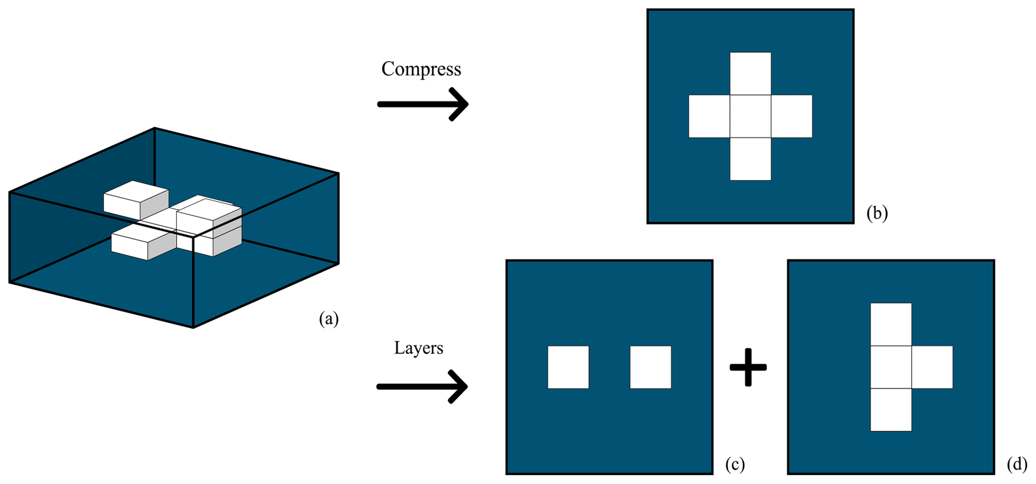
Figure 7Example comparison of two methods of measuring perimeters of a 3D cloud in SAM. The “compressed” method creates a 2D image by vertically summing cloud properties, resulting in a single image for each volume representing how clouds might be seen from above. In contrast, the “layers” method used in Garrett et al. (2018) considers each horizontal slice as a separate image such that for n horizontal layers, n individual images would be produced and analyzed as independent images. In the example, the “compressed” method would produce one cloud with p=12 pixels, and the “layers” method would produce three clouds, one with p=10 and two with p=4.
The difference between the two perspectives can be manufactured in SAM by creating vertically compressed images as they might be seen by a satellite from above. Here, this is accomplished by creating a 2D vertically summed optical depth (τ) field, to which a range of optical depth thresholds are applied to create a selection of cloud masks. Once binary cloud masks are created, clouds are identified and analyzed, as described in Sect. 3.3.
Figure 8 shows that values of β, calculated using the “layer” method in SAM, are consistent with the theoretical prediction β=1 regardless of the threshold used to define clouds; however, the value of β does indeed increase when the perspective is switched to one in which the clouds are vertically compressed as they might be seen from space.
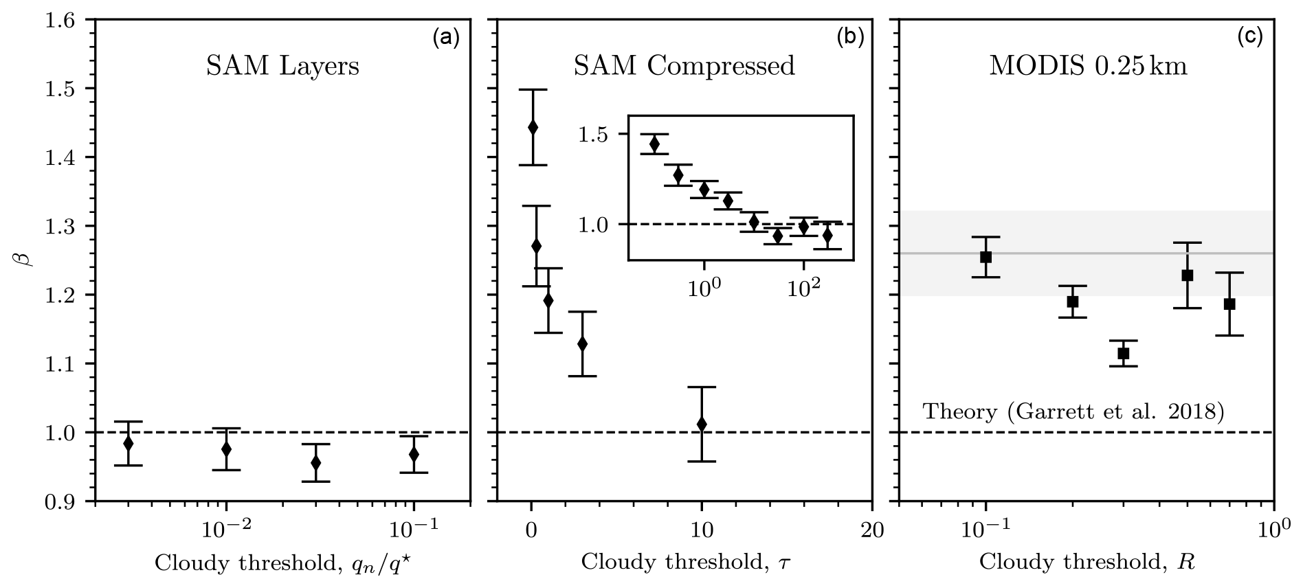
Figure 8(a) Measurements of β for individual horizontal layers (“layers”) in SAM for varying thresholds in total cloud condensate qn, normalized by the saturated mixing ratio q⋆. (b) Measured values of β for “compressed” images in SAM for varying model τ thresholds, created by vertically summing modeled τ. The middle inset displays β vs. τ for the compressed SAM data, using a logarithmically scaled abscissa, over a larger range in τ. (c) Measured values of β for cloud masks of varying reflectance (R) thresholds for MODIS 0.25 km data. See Fig. 7 for a visualization of the difference between “compressed” images and “layers”. The gray line and box indicate the global mean (Fig. 3). Histograms from which values for β are calculated are shown in Sect. S2 in the Supplement.
On the other hand, as the compressed threshold in τ grows, β decreases, reaching a value of roughly 1 at τ≳10. Such sensitivity of β to optical depth threshold is at odds with observations, given that cloud masks specified by thresholds in reflectance between R=0.1 and R=0.7 for MODIS 0.25 km data show very little trend in calculated β. Note, for comparison, that the range of reflectance thresholds considered is roughly equivalent to a range of optical depths between τ=1 and τ=10 and that the reflectance thresholds in MODIS 0.25 km data generally produce values of β that are consistent with the global mean value derived from the pre-processed MODIS cloud mask.
By considering cloud edges as a surface across which cloudy and clear skies compete for available convective potential energy through small-scale mixing processes in a “mixing engine”, Garrett et al. (2018) derived a cloud perimeter distribution that follows a power law , where β=1 (Eq. 3), for perimeters evaluated within thin isentropic layers. The prediction is independent of such considerations as the details of cloud microphysics or climatological state. We find in a detailed numerical simulation of a tropical cloud field that , which is consistent with the prediction.
In a wide range of satellite observations, however, the picture is more nuanced. Within measurement uncertainty, values of β are insensitive to zonal band, land–ocean contrasts, and season, conditionally supporting the small-scale mixing engine hypothesis. However, the globally averaged value across all satellite datasets is significantly higher than predicted by either theory or models, with a value of .
The discrepancy likely owes to a difference in perspective between cloud size distributions measured within individual quasi-horizontal moist isentropic layers, as was done with the numerical simulation, and those seen looking from above, as was calculated using satellite observations. The precise explanation remains a puzzle. We do see that values of β are higher in numerical simulations when the perspective is changed to one looking from above where clouds are defined by a threshold in vertically summed optical depth. This may seem to help resolve the matter. But even here the picture is unclear since β approaches unity as the optical depth threshold increases, and there is no similar sensitivity to reflectance threshold seen in MODIS observations.
Our results also suggest a warning for how future satellite missions are designed. The data compression algorithm used prior to transmission of EPIC data averages 2×2 pixel regions and then interpolates them back to the original resolution in post-processing. We argue that this approach may produce erroneous cloud size distributions that do not follow a power law. Further work could determine whether the interpolation adversely impacts other calculated cloud properties.
Regardless, scale invariance appears to be a defining feature of clouds over at least 4 orders of magnitude in perimeter and 5 in area. We find, in satellite observations, that the upper limit of scale invariance in cloud area distributions amax has a value larger than 3×10⁵ km2, a scale much larger than some other studies have suggested (e.g., Cahalan and Joseph, 1989; Benner and Curry, 1998; Neggers et al., 2003) and close to that found in Wood and Field (2011).
The distribution of cloud areas at large scales remains difficult to measure due to domain size limitations. An intriguing possibility might be to synthesize geostationary data to produce a quasi-global cloud mask product. The product would be similar to existing aerosol optical depth maps (Ceamanos et al., 2021).
With a better understanding of cloud perimeter and area distributions, at least statistically speaking, it may only be necessary to simulate the counts of the largest clouds to predict the numbers of the smallest.
Due to the inaccuracy of measuring cloud perimeters and areas consisting of a small number of pixels (Christensen and Driver, 2021), we remove all clouds with perimeters ≤ 10 × (nadir resolution) or areas ≤ 10 × (nadir resolution)2 (Sect. 3.3). If these same minimum thresholds are used for EPIC's cloud size distributions, results show non-power-law size distributions for both area and perimeter at the small end of the size distribution (Fig. A1). This is in contrast to all other satellite datasets over similar size ranges (Figs. 2 and 3).
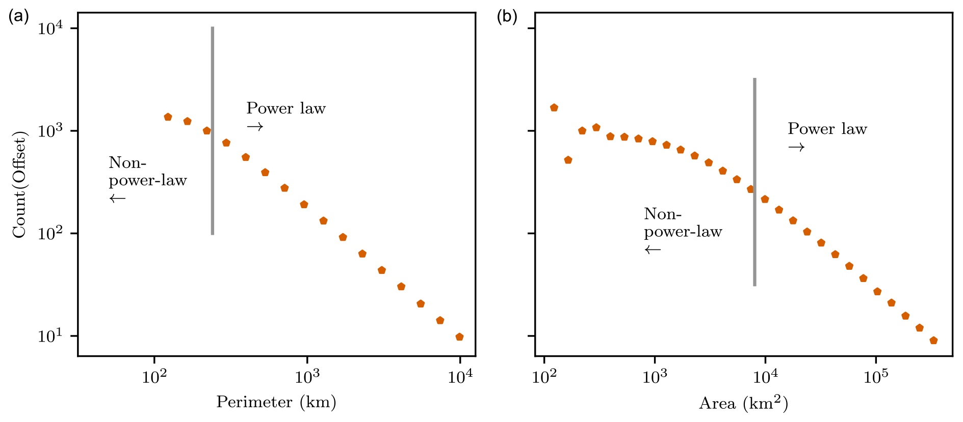
Figure A1Cloud perimeter (a) and area (b) histograms for EPIC, omitting data with perimeters ≤ 10 × (nadir resolution) or areas ≤ 10 × (nadir resolution)2. These thresholds are the same as those used for other datasets; however, EPIC displays non-power-law behavior over the range left of the gray lines. In Figs. 2 and 3, we instead use the gray lines as minimum thresholds (that is, we omit perimeters ≤ 30 × (nadir resolution) or areas ≤ 1000 × (nadir resolution)2).
As a possible explanation for this discrepancy, EPIC imagery is compressed prior to transmission to Earth by averaging 2×2 pixel regions. These regions are then interpolated back to their original resolution in post-processing, artificially smoothing out the details of cloud perimeters. Since cloud perimeter lengths are resolution-dependent, this results in an inaccurate perimeter measurement given EPIC's resolution. Likewise, if the cloud signal in a cloudy pixel is “spread out” into neighboring clear pixels by the smoothing process, pixels that were originally cloudy may become clear or vice versa, so individual cloud areas are likely not conserved through the compression process. Conceivably, these effects may explain the anomalous EPIC area and perimeter distributions, though other differences in, for example, the cloud masking algorithm used may contribute.
It appears that interpolation predominately affects measurements of area and perimeter in small clouds. To account for this inconsistency, we instead truncate EPIC's size distributions where perimeters ≤ 30 × (nadir resolution) or areas ≤ 1000 × (nadir resolution)2. With these revised thresholds, results from EPIC roughly agree with those from other datasets (Figs. 2 and 3).
Python code to analyze all data and generate all figures is available from the first author upon request. The VIIRS and EPIC datasets were downloaded from NASA Earthdata (https://www.earthdata.nasa.gov/, NASA, 2023) and all others from the ICARE Data Center in Lille, France (https://www.icare.univ-lille.fr/, ICARE, 2023).
The supplement related to this article is available online at: https://doi.org/10.5194/acp-24-109-2024-supplement.
TDD: formal analysis, methodology, writing (original draft preparation). TJG: conceptualization, funding acquisition, supervision, methodology, writing (review and editing). KNR: methodology, writing (review and editing). CB: methodology, writing (review and editing). SKK: funding acquisition, writing (review and editing). NF: formal analysis.
At least one of the (co-)authors is a member of the editorial board of Atmospheric Chemistry and Physics. The peer-review process was guided by an independent editor, and the authors also have no other competing interests to declare.
Publisher’s note: Copernicus Publications remains neutral with regard to jurisdictional claims made in the text, published maps, institutional affiliations, or any other geographical representation in this paper. While Copernicus Publications makes every effort to include appropriate place names, the final responsibility lies with the authors.
The Laboratoire d’Optique Atmosphérique kindly hosted visits by Thomas D. DeWitt and Timothy J. Garrett to l'Université de Lille in support of scientific collaboration. The AERIS/ICARE Data and Services Center at l'Université de Lille and the Center for High Performance Computing at the University of Utah provided data storage and computing services. Simon R. Proud and two anonymous referees provided constructive feedback about the manuscript during the interactive discussion phase.
This research has been supported by the National Science Foundation (grant no. 2022941).
This paper was edited by Corinna Hoose and reviewed by two anonymous referees.
Ackerman, S. A., Strabala, K., Menzel, W., Frey, R., Moeller, C., and Gumley, L.: Discriminating clear sky from clouds with MODIS, J. Geophys. Res., 103, 32141–32157, 1998. a, b
Ackerman, S. A., Holz, R. E., Frey, R., Eloranta, E. W., Maddux, B. C., and McGill, M.: Cloud detection with MODIS. Part II: Validation, J. Atmos. Ocean. Tech., 25, 1073–1086, 2008. a
Arakawa, A.: The cumulus parameterization problem: Past, present, and future, J. Climate, 17, 2493–2525, 2004. a
Arakawa, A. and Schubert, W. H.: Interaction of a Cumulus Cloud Ensemble with the Large-Scale Environment, Part I, J. Atmos. Sci., 31, 674–701, https://doi.org/10.1175/1520-0469(1974)031<0674:IOACCE>2.0.CO;2, 1974. a
Arias, P., Bellouin, N., Coppola, E., Jones, R., Krinner, G., Marotzke, J., Naik, V., Palmer, M., Plattner, G.-K., Rogelj, J., Rojas, M., Sillmann, J., Storelvmo, T., Thorne, P., Trewin, B., Achuta Rao, K., Adhikary, B., Allan, R., Armour, K., Bala, G., Barimalala, R., Berger, S., Canadell, J., Cassou, C., Cherchi, A., Collins, W., Collins, W., Connors, S., Corti, S., Cruz, F., Dentener, F., Dereczynski, C., Di Luca, A., Diongue Niang, A., Doblas-Reyes, F., Dosio, A., Douville, H., Engelbrecht, F., Eyring, V., Fischer, E., Forster, P., Fox-Kemper, B., Fuglestvedt, J., Fyfe, J., Gillett, N., Goldfarb, L., Gorodetskaya, I., Gutierrez, J., Hamdi, R., Hawkins, E., Hewitt, H., Hope, P., Islam, A., Jones, C., Kaufman, D., Kopp, R., Kosaka, Y., Kossin, J., Krakovska, S., Lee, J.-Y., Li, J., Mauritsen, T., Maycock, T., Meinshausen, M., Min, S.-K., Monteiro, P., Ngo-Duc, T., Otto, F., Pinto, I., Pirani, A., Raghavan, K., Ranasinghe, R., Ruane, A., Ruiz, L., Sallée, J.-B., Samset, B., Sathyendranath, S., Seneviratne, S., Sörensson, A., Szopa, S., Takayabu, I., Tréguier, A.-M., van den Hurk, B., Vautard, R., von Schuckmann, K., Zaehle, S., Zhang, X., and Zickfeld, K.: Technical Summary, 33–144, Cambridge University Press, Cambridge, United Kingdom and New York, NY, USA, https://doi.org/10.1017/9781009157896.002, 2021. a
Batista-Tomás, A., Díaz, O., Batista-Leyva, A., and Altshuler, E.: Classification and dynamics of tropical clouds by their fractal dimension, Q. J. Roy. Meteor. Soc., 142, 983–988, 2016. a, b, c
Benner, T. C. and Curry, J. A.: Characteristics of small tropical cumulus clouds and their impact on the environment, J. Geophys. Res.-Atmos., 103, 28753–28767, 1998. a, b, c, d, e
Buriez, J. C., Vanbauce, C., Parol, F., Goloub, P., Herman, M., Bonnel, B., Fouquart, Y., Couvert, P., and Seze, G.: Cloud detection and derivation of cloud properties from POLDER, Int. J. Remote Sens., 18, 2785–2813, https://doi.org/10.1080/014311697217332, 1997. a, b
Cahalan, R. F. and Joseph, J. H.: Fractal statistics of cloud fields, Mon. Weather Rev., 117, 261–272, 1989. a, b, c, d, e, f, g, h, i, j
Ceamanos, X., Six, B., and Riedi, J.: Quasi-Global Maps of Daily Aerosol Optical Depth From a Ring of Five Geostationary Meteorological Satellites Using AERUS-GEO, J. Geophys. Res.-Atmos., 126, e2021JD034906, https://doi.org/10.1029/2021JD034906, 2021. a
Christensen, H. M. and Driver, O. G.: The Fractal Nature of Clouds in Global Storm-Resolving Models, Geophys. Res. Lett., 48, e2021GL095746, https://doi.org/10.1029/2021GL095746, 2021. a, b, c, d, e, f, g, h, i
Clauset, A., Shalizi, C. R., and Newman, M. E.: Power-law distributions in empirical data, SIAM Rev., 51, 661–703, 2009. a, b
Cohen, B. G. and Craig, G. C.: Fluctuations in an equilibrium convective ensemble. Part II: Numerical experiments, J. Atmos. Sci., 63, 2005–2015, 2006. a
Craig, G. C. and Cohen, B. G.: Fluctuations in an equilibrium convective ensemble. Part I: Theoretical formulation, J. Atmos. Sci., 63, 1996–2004, 2006. a
Derrien, M. and Gléau, H. L.: MSG/SEVIRI cloud mask and type from SAFNWC, Int. J. Remote Sens., 26, 4707–4732, https://doi.org/10.1080/01431160500166128, 2005. a, b, c, d, e
Derrien, M. and Gléau, H. L.: Improvement of cloud detection near sunrise and sunset by temporal-differencing and region-growing techniques with real-time SEVIRI, Int. J. Remote Sens., 31, 1765–1780, https://doi.org/10.1080/01431160902926632, 2010. a, b, c, d, e
Emanuel, K. A.: The theory of hurricanes, Annu. Rev. Fluid Mech., 23, 179–196, 1991. a
Garrett, T. J.: Modes of growth in dynamic systems, P. Roy. Soc. A-Math. Phy., 468, 2532–2549, https://doi.org/10.1098/rspa.2012.0039, 2012. a
Garrett, T. J., Glenn, I. B., and Krueger, S. K.: Thermodynamic constraints on the size distributions of tropical clouds, J. Geophys. Res.-Atmos., 123, 8832–8849, 2018. a, b, c, d, e, f, g, h, i, j, k, l, m, n, o, p
Glenn, I. B. and Krueger, S. K.: Downdrafts in the near cloud environment of deep convective updrafts, J. Adv. Model. Earth Sy., 6, 1–8, 2014. a
Hanel, R., Corominas-Murtra, B., Liu, B., and Thurner, S.: Fitting power-laws in empirical data with estimators that work for all exponents, PloS one, 12, e0170920, https://doi.org/10.1371/journal.pone.0170920, 2017. a
Heus, T. and Jonker, H. J.: Subsiding shells around shallow cumulus clouds, J. Atmos. Sci., 65, 1003–1018, 2008. a, b
Heus, T., J. Pols, C. F., J. Jonker, H. J., A. Van den Akker, H. E., and Lenschow, D. H.: Observational validation of the compensating mass flux through the shell around cumulus clouds, Q. J. Roy. Meteor. Soc., 135, 101–112, 2009. a
ICARE: ICARE Data and Services Center, ICARE [data set], https://www.icare.univ-lille.fr/, last access: 1 March 2023. a
Imre, A.: Problems of measuring the fractal dimension by the slit-island method, Scripta Metall. Mater., 27, 1713–1716, 1992. a
Khairoutdinov, M. F. and Randall, D. A.: Cloud resolving modeling of the ARM summer 1997 IOP: Model formulation, results, uncertainties, and sensitivities, J. Atmos. Sci., 60, 607–625, 2003. a
Khairoutdinov, M. F., Krueger, S. K., Moeng, C.-H., Bogenschutz, P. A., and Randall, D. A.: Large-Eddy Simulation of Maritime Deep Tropical Convection, J. Adv. Model. Earth Sy., 1, 15, https://doi.org/10.3894/JAMES.2009.1.15, 2009. a, b, c
Kopp, T. J., Thomas, W., Heidinger, A. K., Botambekov, D., Frey, R. A., Hutchison, K. D., Iisager, B. D., Brueske, K., and Reed, B.: The VIIRS Cloud Mask: Progress in the first year of S-NPP toward a common cloud detection scheme, J. Geophys. Res.-Atmos., 119, 2441–2456, https://doi.org/10.1002/2013JD020458, 2014. a
Koren, I., Oreopoulos, L., Feingold, G., Remer, L. A., and Altaratz, O.: How small is a small cloud?, Atmos. Chem. Phys., 8, 3855–3864, https://doi.org/10.5194/acp-8-3855-2008, 2008. a, b
Kuo, K.-S., Welch, R. M., Weger, R. C., Engelstad, M. A., and Sengupta, S.: The three-dimensional structure of cumulus clouds over the ocean: 1. Structural analysis, J. Geophys. Res.-Atmos., 98, 20685–20711, 1993. a, b
López, R. E.: The lognormal distribution and cumulus cloud populations, Mon. Weather Rev., 105, 865–872, 1977. a
Lord, S. J.: Interaction of a Cumulus Cloud Ensemble with the Large-Scale Environment. Part III: Semi-Prognostic Test of the Arakawa-Schubert Cumulus Parameterization, J. Atmos. Sci., 39, 88–103, https://doi.org/10.1175/1520-0469(1982)039<0088:IOACCE>2.0.CO;2, 1982. a
Lord, S. J. and Arakawa, A.: Interaction of a Cumulus Cloud Ensemble with the Large-Scale Environment. Part II, J. Atmos. Sci., 37, 2677–2692, https://doi.org/10.1175/1520-0469(1980)037<2677:IOACCE>2.0.CO;2, 1980. a
Lovejoy, S.: Area-perimeter relation for rain and cloud areas, Science, 216, 185–187, 1982. a, b, c, d
Lovejoy, S.: The Future of Climate Modelling: Weather Details, Macroweather Stochastics – Or Both?, Meteorology, 1, 414–449, https://doi.org/10.3390/meteorology1040027, 2022. a
Maddux, B., Ackerman, S., and Platnick, S.: Viewing geometry dependencies in MODIS cloud products, J. Atmos. Ocean. Tech., 27, 1519–1528, 2010. a
Mandelbrot, B. B.: The fractal geometry of nature, Vol. 1, WH freeman New York, 1982. a
NASA: NASA Earthdata, NASA [data set], https://www.earthdata.nasa.gov/, last access: 1 March 2023. a
Neggers, R., Griewank, P., and Heus, T.: Power-law scaling in the internal variability of cumulus cloud size distributions due to subsampling and spatial organization, J. Atmos. Sci., 76, 1489–1503, 2019. a
Neggers, R. A., Jonker, H. J., and Siebesma, A.: Size statistics of cumulus cloud populations in large-eddy simulations, J. Atmos. Sci., 60, 1060–1074, 2003. a, b, c, d
Newman, M. E.: Power laws, Pareto distributions and Zipf's law, Contemp. Phys., 46, 323–351, 2005. a
Palmer, T. N.: A personal perspective on modelling the climate system, P. Roy. Soc. A-Math. Phy., 472, 20150772, https://doi.org/10.1098/rspa.2015.0772, 2016. a
Peters, O., Neelin, J. D., and Nesbitt, S. W.: Mesoscale convective systems and critical clusters, J. Atmos. Sci., 66, 2913–2924, 2009. a, b, c
Procyk, R., Lovejoy, S., and Hébert, R.: The fractional energy balance equation for climate projections through 2100, Earth Syst. Dynam., 13, 81–107, https://doi.org/10.5194/esd-13-81-2022, 2022. a
Randall, D. A.: Conditional Instability of the First Kind Upside-Down, J. Atmos. Sci., 37, 125–130, https://doi.org/10.1175/1520-0469(1980)037<0125:CIOTFK>2.0.CO;2, 1980. a
Schär, C., Fuhrer, O., Arteaga, A., Ban, N., Charpilloz, C., Di Girolamo, S., Hentgen, L., Hoefler, T., Lapillonne, X., Leutwyler, D., Osterried, K., Panosetti, D., Rüdisühli, S., Schlemmer, L., Schulthess, T. C., Sprenger, M., Ubbiali, S., and Wernli, H.: Kilometer-scale climate models: Prospects and challenges, B. Am. Meteorol. Soc., 101, E567–E587, 2020. a
Schroeder, D.: An Introduction to Thermal Physics, Oxford University Press, ISBN 9780192895547, 2021. a
Siebesma, A. and Jonker, H.: Anomalous scaling of cumulus cloud boundaries, Phys. Rev. Lett., 85, 214–217, https://doi.org/10.1103/PhysRevLett.85.214, 2000. a, b
Slingo, J., Bates, P., Bauer, P., Belcher, S., Palmer, T., Stephens, G., Stevens, B., Stocker, T., and Teutsch, G.: Ambitious partnership needed for reliable climate prediction, Nat. Clim. Change, 12, 499–503, 2022. a
Tennekes, H. and Lumley, J. L.: A first course in turbulence, MIT press, https://doi.org/10.7551/mitpress/3014.001.0001, 1972. a
Wang, Y., Geerts, B., and French, J.: Dynamics of the cumulus cloud margin: An observational study, J. Atmos. Sci., 66, 3660–3677, 2009. a
White, E. P., Enquist, B. J., and Green, J. L.: On Estimating the Exponent Of Power-Law Frequency Distributions, Ecology, 89, 905–912, https://doi.org/10.1890/07-1288.1, 2008. a
Wood, R. and Field, P. R.: The distribution of cloud horizontal sizes, J. Climate, 24, 4800–4816, 2011. a, b, c, d, e, f, g
Xu, K.-M. and Emanuel, K. A.: Is the Tropical Atmosphere Conditionally Unstable?, Mon. Weather Rev., 117, 1471–1479, https://doi.org/10.1175/1520-0493(1989)117<1471:ITTACU>2.0.CO;2, 1989. a
Yamaguchi, T. and Feingold, G.: On the size distribution of cloud holes in stratocumulus and their relationship to cloud-top entrainment, Geophys. Res. Lett., 40, 2450–2454, 2013. a, b
Yang, Y., Meyer, K., Wind, G., Zhou, Y., Marshak, A., Platnick, S., Min, Q., Davis, A. B., Joiner, J., Vasilkov, A., Duda, D., and Su, W.: Cloud products from the Earth Polychromatic Imaging Camera (EPIC): algorithms and initial evaluation, Atmos. Meas. Tech., 12, 2019–2031, https://doi.org/10.5194/amt-12-2019-2019, 2019. a
- Abstract
- Introduction
- A steady-state thermodynamic model for cloud size distributions
- Methods
- Measured cloud size distributions
- Discussion
- Conclusions
- Appendix A: EPIC data
- Code and data availability
- Author contributions
- Competing interests
- Disclaimer
- Acknowledgements
- Financial support
- Review statement
- References
- Supplement