the Creative Commons Attribution 4.0 License.
the Creative Commons Attribution 4.0 License.
 | 07 Sep 2023
Constraints on simulated past Arctic amplification and lapse rate feedback from observations
Olivia Linke
Johannes Quaas
Finja Baumer
Sebastian Becker
Jan Chylik
Sandro Dahlke
André Ehrlich
Dörthe Handorf
Christoph Jacobi
Heike Kalesse-Los
Luca Lelli
Sina Mehrdad
Roel A. J. Neggers
Johannes Riebold
Pablo Saavedra Garfias
Niklas Schnierstein
Matthew D. Shupe
Chris Smith
Gunnar Spreen
Baptiste Verneuil
Kameswara S. Vinjamuri
Marco Vountas
Manfred Wendisch
The Arctic has warmed more rapidly than the global mean during the past few decades. The lapse rate feedback (LRF) has been identified as being a large contributor to the Arctic amplification (AA) of climate change. This particular feedback arises from the vertically non-uniform warming of the troposphere, which in the Arctic emerges as strong near-surface and muted free-tropospheric warming. Stable stratification and meridional energy transport are two characteristic processes that are evoked as causes for this vertical warming structure. Our aim is to constrain these governing processes by making use of detailed observations in combination with the large climate model ensemble of the sixth Coupled Model Intercomparison Project (CMIP6). We build on the result that CMIP6 models show a large spread in AA and Arctic LRF, which are positively correlated for the historical period of 1951–2014. Thus, we present process-oriented constraints by linking characteristics of the current climate to historical climate simulations. In particular, we compare a large consortium of present-day observations to co-located model data from subsets that show a weak and strong simulated AA and Arctic LRF in the past. Our analyses suggest that the vertical temperature structure of the Arctic boundary layer is more realistically depicted in climate models with weak (w) AA and Arctic LRF (CMIP6/w) in the past. In particular, CMIP6/w models show stronger inversions in the present climate for boreal autumn and winter and over sea ice, which is more consistent with the observations. These results are based on observations from the year-long Multidisciplinary Drifting Observatory for the Study of Arctic Climate (MOSAiC) expedition in the central Arctic, long-term measurements at the Utqiaġvik site in Alaska, USA, and dropsonde temperature profiling from aircraft campaigns in the Fram Strait. In addition, the atmospheric energy transport from lower latitudes that can further mediate the warming structure in the free troposphere is more realistically represented by CMIP6/w models. In particular, CMIP6/w models systemically simulate a weaker Arctic atmospheric energy transport convergence in the present climate for boreal autumn and winter, which is more consistent with fifth generation reanalysis of the European Centre for Medium-Range Weather Forecasts (ERA5). We further show a positive relationship between the magnitude of the present-day transport convergence and the strength of past AA. With respect to the Arctic LRF, we find links between the changes in transport pathways that drive vertical warming structures and local differences in the LRF. This highlights the mediating influence of advection on the Arctic LRF and motivates deeper studies to explicitly link spatial patterns of Arctic feedbacks to changes in the large-scale circulation.
- Article
(3043 KB) - Full-text XML
- BibTeX
- EndNote


The Arctic region has warmed more rapidly than the global average during the past few decades, which is seen in both observations and model simulations (e.g. Serreze and Francis, 2006; Serreze et al., 2009; Screen and Simmonds, 2010; Polyakov et al., 2012; Stroeve et al., 2012; Wang and Overland, 2012; Cohen et al., 2014). The most recent period of this Arctic amplification (AA) of climate change started from the end of the 20th century and continues into the 21st century (Overland et al., 2008; Serreze and Barry, 2011; Wendisch et al., 2023). Several intertwined processes and feedback mechanisms give rise to AA, including surface albedo and temperature feedback systems (e.g. Pithan and Mauritsen, 2014; Block et al., 2020). Here we focus on the lapse rate feedback (LRF), which arises from the vertically non-uniform contribution to the total temperature feedback. The LRF contributes at a level that is similar to the surface albedo feedback to AA, but its underlying physical mechanisms are less well understood (Feldl et al., 2020; Lauer et al., 2020; Boeke et al., 2021). Results from the recent multiclimate model ensemble within the sixth Coupled Model Intercomparison Project (CMIP6; Eyring et al., 2016) confirm that the LRF has a unique latitudinal dependence. The multimodel average in Fig. 1a shows a negative LRF in the tropics and large parts of the mid-latitudes and a positive LRF in the polar regions, primarily the Arctic. Most of the negative feedback contribution comes from the tropical regions, where the warming is amplified in higher altitudes. This enhances the outgoing long-wave radiation and thus the atmospheric cooling ability towards space.
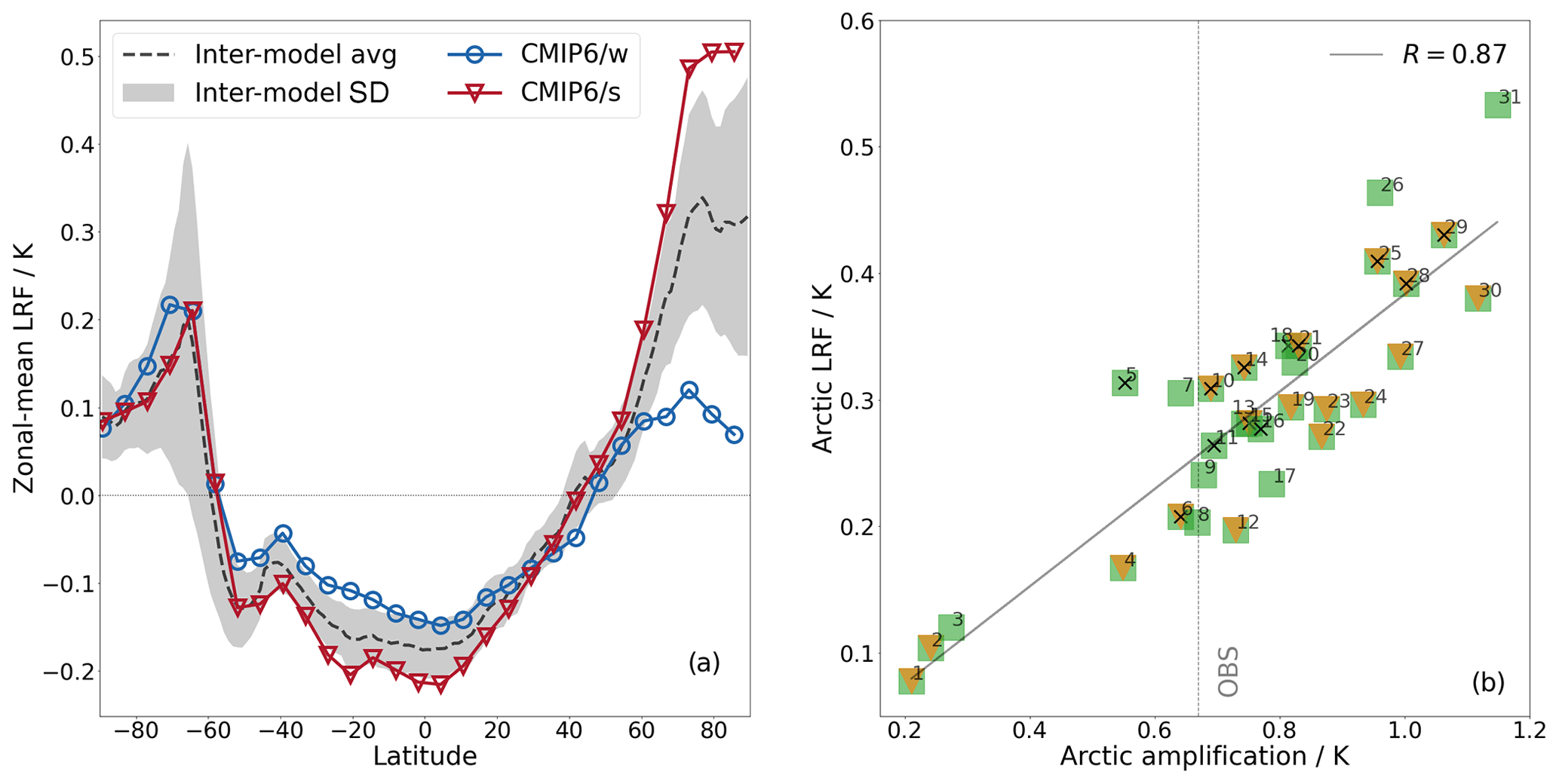
Figure 1(a) Zonal and annual mean LRF (for the period 1985–2014, with respect to 1951–1980) expressed in surface temperature change units (K). The dashed black line indicates the multimodel average (avg) from all 31 CMIP6 models used in this study. The shaded area gives the inter-model standard deviation (SD) around the model mean. The blue lines with circles and red lines with triangles give the average of the three models in the ensemble with lowest and highest AA (CMIP6/w and CMIP6/s), i.e. models 1–3 and 29–31 in Table 1, respectively. The LRF is derived as an average from different radiative kernels (CAM5, GFDL AM2, ERA-Interim, and HadGEM3-GA7). (b) Relationship between AA and Arctic LRF (ALRF) in CMIP6 models. As in panel (a), the model-specific temperature change and feedback is derived for the period 1985–2014, with respect to 1951–1980. Green squares represent the models for monthly data, orange triangles for daily data, and black crosses for 6 h output data that are available from the CMIP6 archive. For the derivation of model-specific AA and LRF, monthly diagnostics of all models (the numbering in panel b corresponds to Table 1) have been used. The observational estimate (OBS) gives the averaged AA derived from different observational data sets.
In the Arctic, the prevailing surface-based temperature inversion and limited vertical mixing abilities of the atmosphere cause the majority of the warming to remain in the lower troposphere (Manabe and Wetherald, 1975). This bottom-heavy warming (BHW) is a key feature of the overall positive Arctic LRF (ALRF). Due to the muted warming in the free troposphere, the ALRF decreases the outgoing long-wave radiation, and thus the atmospheric cooling to space, when compared to vertically uniform warming. This reversed sign of the LRF in different parts of the globe is considered to be an important contribution to AA (Pithan and Mauritsen, 2014; Block et al., 2020).
The ALRF experiences a unique seasonal and spatial variability (e.g. Feldl et al., 2020; Boeke et al., 2021). The majority of the overall positive feedback results from the boreal autumn and winter period, where the degree of sea ice retreat has a strong control on the local intensity of the LRF. Local changes in sea ice concentration are of central importance, as they mediate changes in the surface turbulent heat fluxes. Those regions with strong sea ice reductions primarily experience a large increase in upward turbulent heating from the surface over ocean areas, which mediates the local maximum of the seasonal ALRF (Feldl et al., 2020; Linke and Quaas, 2022).
Here, we are interested in the contribution of the LRF to Arctic warming, which has been observed since 1951. Wendisch et al. (2023) report that in the Arctic (defined in their study as the averaged area north of 60∘ N), the period of 1991–2021 was warmer by 1.33 K compared to the reference period 1951–1980, which is more than twice the global mean warming. We make use of the CMIP6 historical simulations with the best estimates of transient climate forcings over the time period of 1850–2014. In our work, we quantify climate change as being the difference between the last 30 years available from historical simulations (1985–2014) and an earlier 30-year period (1951–1980). The resulting AA and ALRF values are expressed in Fig. 1b, which shows the inter-model spread of both quantities that are linearly correlated (r=0.87). We further derive an observational estimate for AA in the form of an average from several data sets (OBS). In this study, we define AA as being the difference between the Arctic (accounting for the area north of 66∘ N) and global mean warming.
Given the strong seasonal and spatial variability in the ALRF, it is useful to distinguish between different seasons and different surface types for a detailed analysis. For the former point, our results are presented for different times of the year, depending on the availability of observational constraints. We distinguish boreal spring, summer, autumn, and the extended winter as April–May–June (AMJ), July–August–September (JAS), October–November (ON), and December–January–February–March (DJFM), respectively. Even though all seasons are considered, we mostly focus on the winter season, where both AA and ALRF are strong. For the latter point of the surface control on the ALRF, it is most relevant whether the atmospheric column is over sea ice or open ocean (Lauer et al., 2020; Boeke et al., 2021). Since we focus mainly on observational constraints over the Arctic ocean, we exclude the influence of snow-covered vs. snow-free land here. It is further relevant for the evolution of the atmospheric temperature profile to distinguish between the clear and cloudy states of the Arctic atmosphere. In the clear state, strong inversions can evolve, and radiative cooling occurs at the surface. With clouds forming, radiative cooling occurs in the cloud layer rather than at the surface, which ultimately weakens the inversion (Pithan et al., 2014).
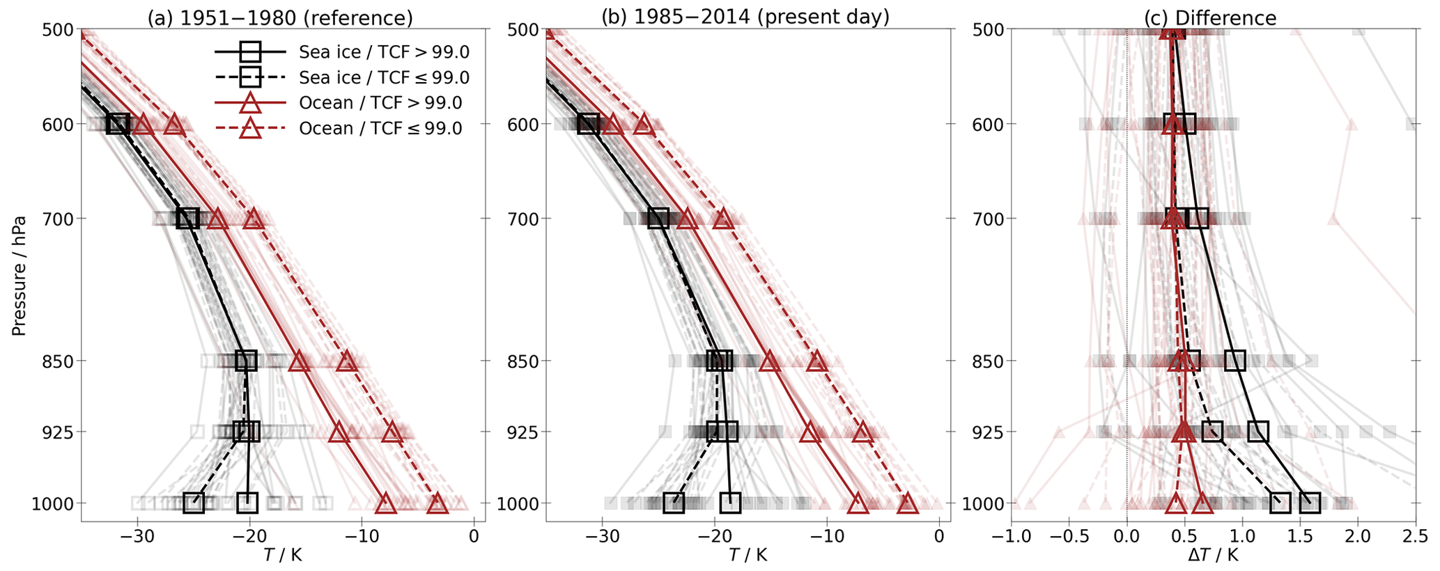
Figure 2Temperature profiles derived from monthly mean CMIP6 data for (a) the reference period 1951–1980, (b) the present-day period 1985–2014, and (c) the difference between the later and earlier period, respectively. The season is DJFM. Temperature profiles are derived over sea ice and ocean surfaces for overcast conditions with the total cloud fraction (TCF) > 99 % and non-overcast conditions with TCF ≤ 99 % in the columnar monthly mean files, respectively. The sea ice concentration threshold is 15 %, above which we define the ocean surface as being covered by sea ice. Model grid points are selected as either sea ice or open ocean in contexts where these conditions are fulfilled for both reference and present-day period, respectively. The difference profiles in panel (c) are derived from grid points for which these conditions are true for both reference and present-day period, respectively. The curves show the multimodel average (thicker curves) and individual models (thin shaded curves). Note that not all 31 models are included here, as not every model gave an output profile for each of the four classifications according to surface type and cloudiness.
We first motivate the influence of both surface type and cloudiness on the ALRF during the extended winter using only CMIP6 data. Figure 2 shows temperature profiles in the lower and middle troposphere that is filtered for different conditions. Profiles are categorised into two surface types (sea ice or ocean) and two cloud conditions, which is based upon a threshold in the total cloud fraction (TCF) within the model grid cell (TCF > 99 % or TCF ≤ 99 %). Therefore, we distinguish four different cases, namely sea ice/TCF > 99 %, sea ice/TCF ≤ 99 %, ocean/TCF > 99 %, and ocean/TCF ≤ 99 %. The sea ice concentration threshold of 15 % is used to distinguish sea ice from the open-ocean areas (e.g. Lauer et al., 2020; Boeke et al., 2021; Linke and Quaas, 2022). The categorisation of cloudiness aims to separate the particularly cloudy (overcast) conditions from the rest. We discuss the choice of the TCF threshold later on in the text.
By comparing two different states of cloudiness while considering the same surface type (sea ice or ocean), we at least partly isolate the effect of cloudiness on the temperature profile and its changes. On the other hand, by comparing two different surface types while considering the same state of cloudiness (overcast or non-overcast), we at least partly isolate the effect of different surface types on the temperature profile and its changes.
By distinguishing according to surface type and cloudiness, we motivate the observational constraints with the following conclusions based on purely model-based outputs.
-
Reference (1951–1980) and present-day (1985–2014) periods. For non-overcast cases (TCF ≤ 99 %), the contrast in surface temperature over sea ice and open ocean dominates the temperature profiles. Over sea ice, strong surface inversions exist, while over the relatively warm ocean, the atmospheric boundary layer is well mixed. For overcast cases (TCF > 99 %), the strong cloud cover reduces the surface temperature contrast between sea ice and open ocean. Over sea ice, cloud-top cooling leads to a top-down mixing of the atmospheric boundary layer, which weakens the surface inversion. Some models show a lifted inversion (e.g. CESM2; not shown). Over open ocean, both cloud conditions show a similar stability, but the highly clouded profile is colder throughout the lower troposphere. This is due to the fact that these cases appear most frequently along the sea ice edge than in other parts of the Arctic (not shown here) when compared to the less clouded profiles over ocean.
-
Present-day period minus reference period. The open-ocean areas show no substantial change in the lapse rate; i.e. there are no strong LRF results from both cloud conditions over open ocean. However, there is a strong warming near the surface over sea ice for both overcast and non-overcast conditions, when compared to over open ocean. The overall warming in the overcast cases is more pronounced than for other conditions, likely due to the fact that these cases mostly appear over the strong ice melt areas of the Barents–Kara seas (not shown here), which have a notoriously strong warming. However, it is only under overcast conditions that this enhanced warming signal extends up into the mid-troposphere. The gradient of the temperature change from the surface to 850 hPa over sea ice is larger under less clouded conditions relative to overcast conditions. Thus, more clouds reduce the bottom-heavy warming with respect to the lower troposphere by up to 850 hPa. However, considering the entire troposphere (extending from the surface to 300 hPa at the poles; Soden and Held, 2006), the overall columnar LRF accounting for the lapse rate change in each layer is stronger for overcast profiles.
Summarising this introduction, state-of-the-art climate models imply a large role of inversion, surface types, and clouds for the evolution of the Arctic temperature profile with warming. In addition, the thermal structure of the atmosphere can be impacted by remote processes like poleward energy transport. Those controls motivate the investigation of whether detailed observations or reanalyses can be used as constraints, based upon the CMIP6 inter-model spread in AA and ALRF (Fig. 1b).
The key ideas are as follows.
-
The Arctic LRF is largely controlled by local influences on the near-surface thermodynamic structure because the lack of vertical mixing in the Arctic boundary layer is key to understanding and adequately modelling the ALRF. As a result, one focus will be on the evaluation of simulated inversion strengths by using various means. Additionally, the ALRF is largely dependent on the underlying surface type. Most importantly, the strong contrast in LRF and local warming over sea ice and open-ocean surfaces motivates an evaluation of the simulated warming that is expected through sea ice retreat.
-
The meridional transport of energy in the Arctic free troposphere undergoes a change due to Arctic warming and may amplify or dampen the ALRF through energy advection at different altitudes.
-
The lapse rate change is linked to the cloudiness and vertical mixing strength in the atmospheric column. A further aim is to motivate an assessment of how clouds and boundary layer dynamics shape changes in the lapse rate through a vertical redistribution of the warming.
We address points 1 and 2 by comparing present-day (or historical changes in) observations or reanalyses with co-located model data. The constraint is based on the separation of the co-located model data into a subset of models with either weak or strong simulated past AA (and ALRF, given their high inter-model correlation; Fig. 1b). By identifying differences between both model subsets, and falsifying either one or the other based upon observations, we link characteristics of the current climate to a long-term historical climate simulation. This allows us to evaluate the performance of CMIP6 models and to constrain parameters linked to both local and remote processes mediating the ALRF and AA. Point 3, which regards the role of clouds and boundary layer dynamics, is treated separately from this process-oriented constraint. Our model-based results in Fig. 2 are thus linked to a deeper study of these perspectives in large-eddy simulations.
We note that this work aims to provide insight to different perspectives on the ALRF and AA. We bring together a variety of contributions from a large research consortium and ultimately seek synergy among them.
In Sect. 2, we first elaborate on how AA and the Arctic LRF are calculated from climate model diagnostics and radiative kernels and on how to facilitate a constraint based upon this. Second, the different observational data sets and individual methods are described. Section 3 evaluates the performance of the two CMIP6 model subsets to simulate parameters linked to processes that can impact the Arctic LRF, based on the observations introduced in Sect. 2. In Sect. 4, we further explain the differences between both model subsets and link our results to the historical climate simulations, which is equivalent to our constraint. Our final conclusions revisit hypotheses 1–3.
To address the objectives of this study, we evaluate the performance of CMIP6 models with a wide range of observables in different parts of the Arctic. From CMIP6, we use historical simulations with the best estimates of the transient climate forcings during 1850–2014 (Eyring et al., 2016). In this study, we focus on the period 1951–2014. For our analyses, we use the entire data set of available CMIP6 data and compute ensemble means over all realisations per model. In this way, each model carries equal weight in the inter-model distribution, and we further exclude the chance of choosing one model realisation that deviates substantially from the entire population. By taking the average of the model realisations over the past few decades, we average out the effect of internal climate variability and isolate the response to external forcing. However, the observations represent a single climate trajectory and thus combine both the effect of internal variability and the forcing response. We therefore also discuss our main results in the context of internal variability (see Sect. 2.9).
Volodin et al. (2019a)Volodin et al. (2019b)Krasting et al. (2018)Ridley et al. (2018)Park and Shin (2019)Neubauer et al. (2019)Scoccimarro et al. (2020)Savita et al. (2019)Hajima et al. (2019)Danek et al. (2020)Bentsen et al. (2019)Danabasoglu (2019a)Xin et al. (2018)Voldoire (2018)Wieners et al. (2019)Tatebe and Watanabe (2018)Ziehn et al. (2019)NASA/GISS (2018a)Tang et al. (2019)Cao and Wang (2019)Jungclaus et al. (2019)Danabasoglu (2019b)Guo et al. (2018)Danabasoglu (2019c)Seferian (2018)Yu (2018)Danabasoglu (2019d)Voldoire (2019)Boucher et al. (2018)Yukimoto et al. (2019)NASA/GISS (2018b)Table 1All CMIP6 models used in this study with AA and ALRF are derived from the near-surface atmospheric temperature and lapse rate difference, respectively, between 1985–2014 and 1951–1980. Table 1 further gives the time resolution available in the model diagnostics (with 6 h, day for daily, and mon for monthly), together with the categorisation of weak or strong AA models (CMIP6/w or CMIP6/s; seen in the superscript of the acronyms) per time resolution group. Model acronyms in bold indicate models that are most skilled at simulating a realistic volume of sea ice loss together with a plausible global temperature change over time according to Notz and the SIMIP Community (2020).
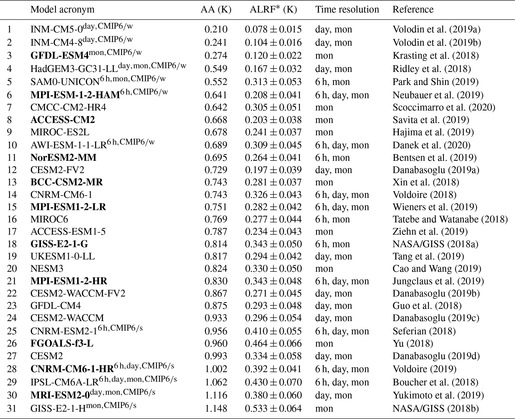
* ALRF values are computed by averaging the results derived from several kernels (CAM5, GFDL AM2, ERA-Interim, and HadGEM3-GA7). The inter-kernel standard deviation gives the error range.
While monthly mean data are available for all CMIP6 models used in this study, only a few models provide all diagnostics necessary for comparing the data at higher time resolutions. Therefore, we define three different model data sets at different time resolutions, namely monthly (all 31 models), daily, and 6 h. We specify the models that provide all necessary diagnostics per time resolution group in Table 1. The model data for each of these time resolution groups are further broken down into a respective subset that simulates either a weak (w) or strong (s) historical AA and ALRF (CMIP6/w or CMIP6/s, respectively). For CMIP6/w and CMIP6/s subsets, we group together the three models with lowest- and highest-simulated AA, respectively (see Table 1 for details). Thus, we largely focus on climate models at the edge of the inter-model range to ensure a clear signal and allow for an attribution to either weak or strong historical AA and ALRF projections. We do not perform a “classic” emergent constraint that seeks strong statistical relationships between aspects of past or future climate simulations and the observable present.
We further use observational estimates to calculate AA and to interpret the simulated model range with respect to observations. The “best” estimate of AA is derived from the AA averages of the NASA Goddard Institute for Space Studies Surface Temperature version 4 (GISTEMP v4), the Berkeley Earth Surface Temperatures (BEST) data set, the Met Office Hadley Centre/Climatic Research Unit version 5.0.1.0 (HadCRUT5), the NOAA Merged Land and Ocean Surface Temperature Analysis (MLOST), and the fifth generation reanalysis of the European Centre for Medium-Range Weather Forecasts (ERA5).
In each comparison step, we use a specific observational data set to evaluate the performance of the respective CMIP6/w and CMIP6/s subset and to constrain one key parameter linked to a characteristic process. The locations of the observational sites are summarised in Fig. 3. The model-to-observation (or model-to-reanalysis) comparisons include the following:
-
We compare temperature inversion strengths measured during the Multidisciplinary Drifting Observatory for the Study of Arctic Climate (MOSAiC; Shupe et al., 2022) to the corresponding CMIP6 data. The colour coding in Fig. 3 shows the drift of the research vessel (R/V) Polarstern during MOSAiC from October 2019 to October 2020. More information is given in Sect. 2.2.
-
Complementary to MOSAiC, we further use inversion data from long-term radiosonde observations at the Atmospheric Radiation Measurement (ARM) site at Utqiaġvik, Alaska, USA (see Sect. 2.3 for details).
-
We further analyse measurements of temperature profiles by dropsondes released from research aircraft during several measurement campaigns in the Fram Strait (grey box in Fig. 3). More information about the campaign data is provided in Sect. 2.4.
-
In the context of remote controls on the ALRF, we relate the depth of the Arctic warming at the observational sites at Utqiaġvik and Fram Strait (red sectors in Fig. 3) with preferred large-scale atmospheric circulation regimes over these regions. Further information is given in Sect. 2.5.
-
To broaden the perspective of advective controls, we derive the pan-Arctic poleward energy transport across the Arctic boundary at 66∘ N, which encloses the entire area illustrated in Fig. 3. The methodology is further specified in Sect. 2.6.
-
Finally, the LRF as a positive radiative feedback in the Arctic locally enhances the greenhouse effect. Therefore, we relate its strength to changes in the long-wave radiation budget at the top of the atmosphere (TOA). Again, we consider the area north of 66∘ N to derive pan-Arctic averages. Details are described in Sect. 2.7.
-
From an outlook perspective, and to augment the observational data sets derived during MOSAiC, we further conducted daily large-eddy simulations (LESs) for the whole MOSAiC drift (Sect. 2.8). These simulations aid in the discussion of processes at turbulence- and cloud-resolving scales, as they are largely underrepresented in the literature covering the Arctic LRF.
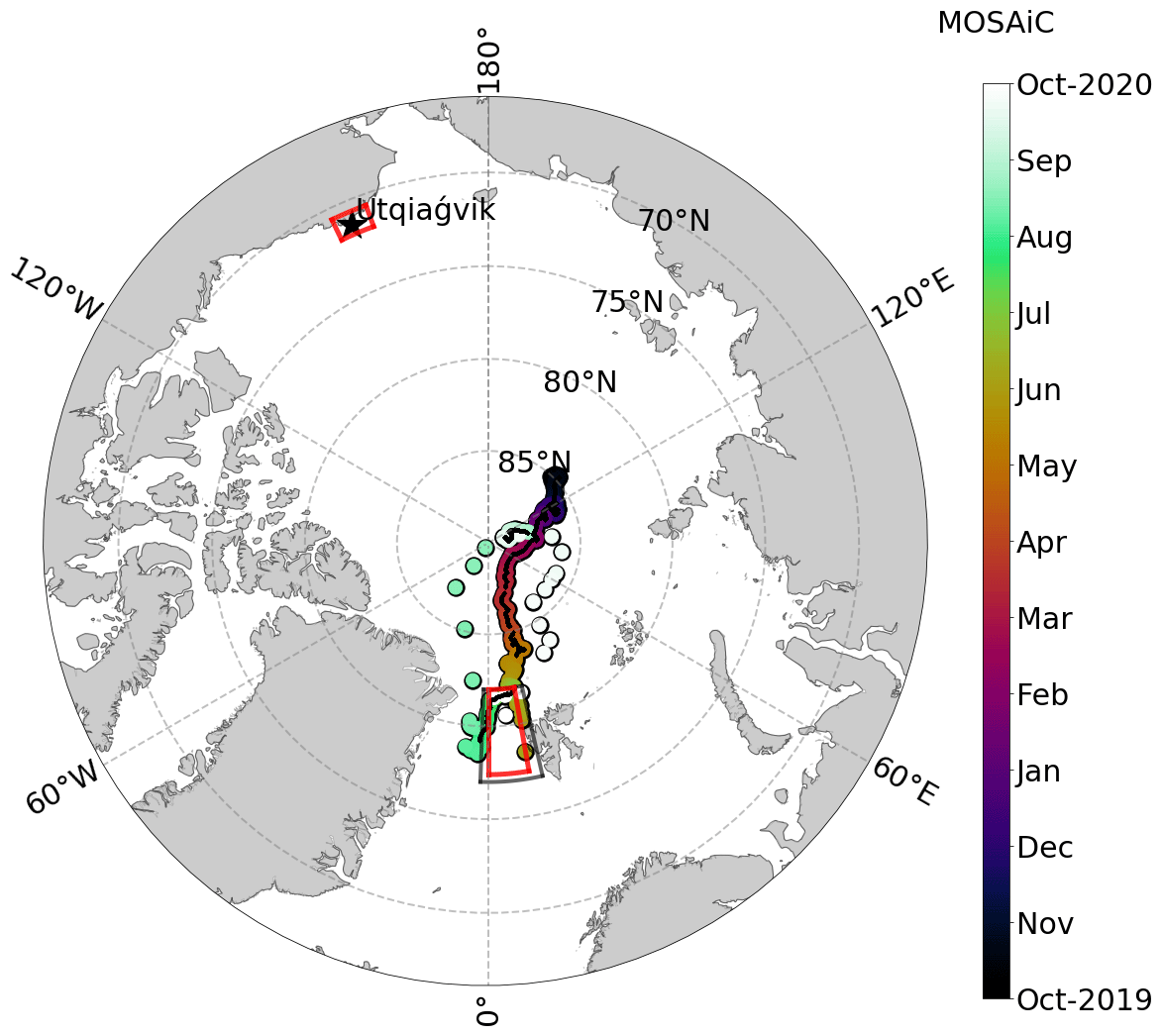
Figure 3The Arctic region north of 66∘ N, which summarises all domains considered for comparing the observations and reanalyses to CMIP6. Colour coding represents the location of the R/V Polarstern drift as a function of time from October 2019 to October 2020 during the MOSAiC expedition. Black dots (appearing as a connected line in the reddish colour range) in the track represent location and time of the observational data set used in this study (Sect. 2.2). The ARM site at Utqiaġvik, Alaska, is marked by a star (Sect. 2.3). The dropsonde domain is the enclosed area in the Fram Strait marked by the dark grey trapezoid (Sect. 2.4). The regions around Utqiaġvik and the Fram Strait that are discussed in Sect. 2.5 are marked by red trapezes. The entire area north of 66∘ N is used for deriving pan-Arctic averages of Arctic LRF and AA (Sect. 2.1). Additionally, we consider the net energy transport across the Arctic boundary and the long-wave radiation budget at the TOA within this area (Sects. 2.6 and 2.7, respectively).
2.1 Arctic amplification and Arctic LRF in CMIP6 models
To facilitate constraints on the past AA and ALRF, we first calculate a model-specific AA and ALRF value from monthly mean temperature fields for all 31 climate models considered in this study. We define the degree of AA by subtracting the global mean near-surface air temperature change, ΔTs, from the respective Arctic mean. Arctic mean values account for the averaged area north of 66∘ N. We chose this metric over defining AA as the ratio of global mean and Arctic warming as the period of interest because some model realisations show a global mean warming that is close to zero. Therefore, the ratio estimator causes the risk to arbitrarily inflate the model spread (Hind et al., 2016; Davy et al., 2018).
Again, the LRF arises from tropospheric warming that is vertically non-uniform. The change in the temperature profile is calculated for the averaged period of the last 30 years of the historical simulations (1985–2014) compared to the period 1951–1980. By choosing that time period, we cover the modern era of AA that has been identified from the second half of the 20th century and that continues into the 21st century (Davy et al., 2018, and references therein). The LRF is derived from pre-computed radiative kernels which give the change in the TOA radiation balance due to a perturbation in the temperature of 1 K. We consider radiative kernels from the CAM5 (Pendergrass, 2017), GFDL AM2 (Feldl et al., 2017), ERA-Interim (Huang et al., 2017), and HadGEM3-GA7 (Smith et al., 2020) climate models. The model-specific LRF is derived as the LRF average, which has been derived from each kernel individually. The corresponding kernel-averaged ALRF values are given in Table 1, with inter-kernel standard deviations as the uncertainty ranges. We want to stress that the inter-model relationship between AA and ALRF is only slightly affected by the choice of kernel, with correlation coefficients of r=0.89, 0.90, 0.91, and 0.92 for HadGEM3-GA7, CAM5, ERA-Interim, and GFDL AM2, respectively. Therefore, our classification of either CMIP6/w or CMIP6/s models is not sensitive to the choice of kernel.
The feedback parameter λ is defined as
with representing the radiative kernel. ΔX gives the change in temperature profile that deviates from ΔTs. The LRF is calculated by applying Eq. (1) and integrating it over the troposphere. We derive the tropopause, following Soden and Held (2006), by defining the 100 hPa pressure level as tropopause at the Equator and using a linear slope (according to geographical latitude) down to 300 hPa at the poles.
The feedback parameter λ has the unit of watts per square metre per kelvin (). We redefine the feedback parameter as a warming contribution to ΔTs by using the local energy budget and following several prior studies (Lu and Cai, 2009; Crook et al., 2011; Feldl and Roe, 2013; Taylor et al., 2013; Pithan and Mauritsen, 2014; Goosse et al., 2018; Hahn et al., 2021):
The local energy budget in Eq. (2) describes the energetic contributions of the radiative forcing F, the feedbacks (λiΔTs), and the Planck response (λPΔTs), as well as the ocean heat uptake (ΔOHU) and the anomalous atmospheric heat transport convergence (ΔAHT). The second step splits the Planck feedback into its global mean value, , and the spatially resolved deviation from it, . Therefore, we can derive the warming contributions to ΔTs from the forcings and feedbacks by dividing each term in Eq. (2) by the global mean Planck feedback (), as follows:
In that form, each of the individual contributions on the right-hand side add up to the full change in Ts. In our study, however, we only consider the contribution of the LRF to ΔTs.
2.2 Temperature inversions during MOSAiC
During the MOSAiC expedition between October 2019 and October 2020, R/V Polarstern drifted within the central Arctic sea ice. During the expedition, vast atmospheric measurements, among others, were carried out (Shupe et al., 2022). In this study, we analyse thermodynamic profiles from Vaisala RS41-SGP radiosondes that were launched at least 4 times per day (Maturilli et al., 2021). In order to estimate the temperature inversions from the soundings, we additionally employ concurrent 2 m temperature (T2m) measurements from the nearby MOSAiC ice camp (Cox et al., 2021), since the soundings were launched from the ship's helicopter deck approximately 10 m above the ice, thus missing the lowermost metres of the atmospheric column. In addition, using the T2m tower data will reduce the impact of the ship on the near-surface temperature. We derive the inversion strength as the difference between the temperature profile maximum (Tmax; between the surface and 250 hPa) and T2m. Each model's vertical resolution is thus maintained without interpolating the profiles to a common pressure coordinate.
The temporal resolution for the inversion data follows the frequency of the radiosonde launches during the MOSAiC expedition (approximately every 6 h). For the model-to-observation comparison, we consider 6 h temperature diagnostics for the period 2010–2014 that were co-located to MOSAiC in the space and time of the year. Since the climate models are free-running coupled models, it is not essential to use the exact years of 2019–2020; instead, the correct time (i.e. time of day and season) and spatial location are co-located. Nevertheless, we justify the model-to-observation comparison by testing the similarity between the model's time series for historical output data 2000–2014 and the highest emission scenario (Shared Socioeconomic Pathway 585 or SSP585) as the upper boundary of available scenarios in CMIP6 (for those models that provide 6 h diagnostics for both simulations; not shown). Our analysis shows that the SSP585 time series consistently lies within the inter-annual range of the 2000–2014 historical data and is, for most of the year, within the range of inter-annual standard deviation, which justifies our approach.
The model output data are chosen to correspond to whichever time step and grid box midpoint is closest to each individual MOSAiC radiosonde launch. Essentially, the model data “follow” the MOSAiC track in the space and time of the year. We thus derive the temperature inversion in the model data as being the difference between Tmax and T2m.
Note that there are no inversion data available for MOSAiC between 9 May 2020 to 10 June 2020 and 29 July 2020 to 25 August 2020, which is when the ship was in transit through the sea ice. Figure 3 shows the entire drift of R/V Polarstern, with the time attribution according to the radiosonde launches shown with colour coding. The black dots following the drift depict the locations where observational data were available for our study (limited by the availability of T2m tower data).
2.3 Temperature inversions at Utqiaġvik (NSA)
The ARM programme organised by the U.S. Department Of Energy (DOE) provides a long-term record of atmospheric observations from permanent and mobile measurement sites around the world (Mather and Voyles, 2013). One ARM site that is particularly relevant for Arctic studies is the northern slope of Alaska (NSA) in Utqiaġvik, Alaska, USA. With a geographical location of 71.23∘ N, 156.61∘ W, the NSA site is one of the most important sources for long-term western Arctic atmospheric observations, which makes it ideal for climate studies.
For this study, we use atmospheric temperature profiles from radiosonde launches performed at the NSA site. The so-called Interpolated Sonde (INTERPSONDE) value-added product is obtained after linearly interpolating the atmospheric state variables from consecutive soundings into a fixed 2-D time–height grid. The grid's temporal resolution is 1 min. The vertical resolutions vary with altitude, ranging from 20 m in the lowest 3.5 km and 50 m between 3.5–5 km to 100 m between 5–7 km and 200 m between 7–20 km altitude, respectively. It is important to mention that the input for the INTERPSONDE product comprises only data from quality-controlled soundings and precipitable water vapour estimated from microwave radiometer measurements, and it does not incorporate ancillary observations from surface or tower meteorological observations. The INTERPSONDE product's fixed 2-D grid facilitates the comparison with weather and climate models. Radiosonde data for the NSA site have been available since April 2002, varying from two to four launches per day (Jensen et al., 1998).
Once the CMIP6 model output and NSA radiosonde data are processed to be comparable, we estimate the temperature inversion strength as for MOSAiC (i.e. the difference between Tmax and T2m at 6 h time resolution).
2.4 Temperature profiles in the Fram Strait
The relationship between the ALRF and the strength of sea ice retreat motivates the assessment of temperature profiles above both sea ice and open-ocean surfaces and the assessment of their differences. For this purpose, measurements of dropsondes released from research aircraft in the Fram Strait are analysed. The dropsondes deliver atmospheric profiles for altitudes below the launch location. The limited flight altitude of the employed research aircraft constrains the maximum altitude of the resulting temperature profiles to about 3 km. Since the measurements presented here are available only for March, we restrict the model-to-observation comparison to this month. However, the thermodynamic conditions are similar when compared to the extended winter season of DJFM (not shown).
In total, 52 dropsondes are analysed, and these were mainly launched in an area between 77–82∘ N and 2∘ W–13∘ E (see Fig. 3) during the following three campaigns: eight sondes during the Radiation and Eddy Flux Experiment (REFLEX; performed in March 1993; Lüpkes and Schlünzen, 1996), 22 sondes during the Springtime Atmospheric Boundary Layer Experiment (STABLE; performed in March 2013; Lüpkes et al., 2021), and 22 sondes during the Airborne measurements of radiative and turbulent FLUXes of energy and momentum in the Arctic boundary layer campaign (AFLUX; performed in March–April 2019; Becker et al., 2020).
For the surface type classification, the sea ice concentration at the dropsonde launch location was obtained from satellite observations (Kern et al., 2020, for REFLEX and Melsheimer and Spreen, 2019, for STABLE and AFLUX). If the sea ice concentration was below 15 %, then the profile is considered to represent conditions over open ocean, while a sea ice concentration above 85 % corresponds to a sea-ice-covered ocean. Thus, we exclude data from six dropsondes that were launched over the marginal sea ice zone (15–85 %) in this analysis, which is designed to obtain a clear signal for the difference between sea ice and open ocean.
As for MOSAiC and NSA, the model-to-observation comparison applies data with 6 h time resolution for 2010–2014 in the model output. Similar to the observations, the temperature profiles from the models were grouped into open-ocean and sea ice conditions, based on the model sea ice concentration at the respective grid cell. The location of the sea ice edge varies significantly among the models. To reduce the impact of the different distances to the sea ice edge on the thermodynamic profile, grid points with a distance of more than 250 km to the 50 % isoline of sea ice concentration are excluded from the analysis.
2.5 The role of local advective heating
The thermodynamic structure of the atmosphere is not only affected by atmospheric stability and sea ice loss but also by remote influences. Here, we link the vertical structure of Arctic warming to large-scale atmospheric circulation regimes over the regions of the Fram Strait and Utqiaġvik (marked in Fig. 3). Again, the years of 1951–1980 are chosen as the reference period, and the years 1985–2014 represent the present-day climate state.
We identify the preferred atmospheric circulation regimes in the reanalysis data by analysing the daily mean sea level pressure (SLP) anomaly fields over the North Atlantic–Eurasian region (30–90∘ N, 90∘ W–90∘ E) and over the North Pacific region (30–90∘ N, 90∘ E–90∘ W) separately for the extended winter season (DJFM). For the reanalysis data, the ERA5 reanalysis is employed (Hersbach et al., 2023). We follow the approach described in Crasemann et al. (2017) and determine the ERA5-based circulation regimes as being non-Gaussian structures in a reduced-state space (Dawson and Palmer, 2015). In more detail, the analysis comprises the following steps: (1) the dimensionality of the data set is reduced by an empirical orthogonal function (EOF) analysis. The subsequent analysis is performed in the reduced-state space spanned by the five leading EOFs (Dawson and Palmer, 2015), which explain about 57.5 % of the variance in the SLP anomaly fields over the North Atlantic–Eurasian region and 54.8 % of the variance over the North Pacific region. The leading EOFs resemble well-known teleconnection patterns such as the North Atlantic Oscillation (NAO), east Atlantic pattern, Pacific–North American pattern, and west Pacific pattern. The coordinates in the reduced-state space are provided by the corresponding non-normalised principal component (PC) time series. We have proven the robustness of the identified regimes with an analysis in the state space that is spanned by the 10 leading EOFs. (2) A k-means clustering has been performed in the reduced-state space, where the number of clusters k has been set to k=5, following Crasemann et al. (2017). These clusters are interpreted as being the preferred circulation regimes, and each time step of the data set has been assigned to one of the clusters. The clusters are characterised by SLP anomaly fields, reconstructed from the 5-dimensional coordinate vectors of the cluster centroids.
For the analysis of the CMIP6 data, we apply a projection approach, as described in Fabiano et al. (2021), where the state space spanned by the ERA5 EOFs serves as the reference state space for the CMIP6 simulations. The coordinates for each simulation are provided by projecting the SLP anomaly data onto the reference state space, thus obtaining five pseudo-PCs for each model simulation. Based on these pseudo-PCs, each day of the respective model simulation is assigned to the closest centroid of the five ERA5 reference clusters. The advantage of this approach is the consistent definition of the atmospheric circulation regimes.
A bootstrap test, similar to that used in Crasemann et al. (2017), was used to test for changes in the relative frequency of occurrence of the regimes between the reference and the present-day period. A significant change in the frequency of occurrence was detected at the 95 % level if no more than 5 % of the 10 000 bootstrap replicates of the time series describing the occurrence of the regimes showed a greater difference than the change in the frequency of occurrence of the original occurrence time series.
In order to relate the occurrence probability of each circulation regime i (Pi, ) to the vertical structure of the warming at the observational sites, we applied a multinomial logistic regression (MNLR) approach. This approach was used by, for example, Detring et al. (2021) to study the recent trends in blocking probabilities, but it is also suitable for the multiclass problem of describing Pi in the dependence of some covariates. The basic idea of MNLR is to describe the log odds (defined as the logarithm of the chance of observing a distinct regime with respect to a predefined baseline regime) as a linear combination of the covariates. For our analysis, the covariates comprise the 2 m temperature (T2m), the mid-tropospheric temperature at 500 hPa (T500), and time. T2m and T500 are averaged values over the region around the respective measurement site.
Finally, the relationship between the occurrence probability of each circulation regime and the warming structure is expressed as a 2-dimensional probability density function (PDF) dependent on the T2m and T500 changes. We henceforward refer to an increase in T2m and T500 with time as bottom-heavy warming and top-heavy warming, respectively. We constrain the remote influence of advective heating on the ALRF by a model-to-reanalysis comparison, using ERA5 and CMIP6 models with daily output data, as specified in Table 1.
We ultimately seek to establish a link between changes in large-scale circulation patterns that mediate vertically non-uniform warming structures and the local magnitude of the LRF in the Arctic. In a second step, we extent this method and focus on the pan-Arctic atmospheric transport in the current climate and its connection to both past AA and ALRF.
2.6 Pan-Arctic atmospheric energy transport convergence
To derive the pan-Arctic atmospheric transport in the present-day climate state, we make use of the large-scale and long-term Arctic atmospheric energy budget (AEB) equation. Following previous works (e.g. Nakamura and Oort, 1988; Trenberth, 1997; Serreze et al., 2007), we can describe the energy budget of any atmospheric column that extends from the surface to the TOA as
which comprises the tendency in energy storage , the net atmospheric radiation budget Ra, the sum of turbulent heat fluxes at the surface QH, and the convergence of the horizontal atmospheric energy transport . The radiation budget Ra is derived from the sum of the net downward radiative flux at the TOA and the upward radiative flux at the surface in both long- and short-wave frequencies, respectively. The net turbulent heat flux at the surface is composed of both sensible and latent heating. The AEB in the form of Eq. (4) is a simplification and does not account for factors like the conversion between liquid water and precipitating ice. However, the residual that arises from these terms is shown to be small in the long-term and annual mean Arctic AEB, just like the storage tendency under the steady-state assumption (Serreze et al., 2007; Linke and Quaas, 2022). The main components that define the long-term and large-scale Arctic AEB are therefore the atmospheric radiation budget, the net surface turbulent heat flux, and the transport term. We apply the same approach as the one in Linke and Quaas (2022) and derive the horizontal convergence of atmospheric energy transport indirectly, i.e. as the residual of Eq. (4). From the indirect method of using the AEB, we do not distinguish either contribution of dry static energy and latent heat transport.
For our constraint, we compare the transport convergence (positive is the net atmospheric transport into the polar cap) at present-day climate state (2000–2014) in a model-to-reanalysis comparison. Due to the larger volume of model data available in the subset with a monthly resolution (Table 1), we further calculate the inter-model correlation coefficients for the entire collection of models.
To determine the statistical significance in our analysis, a bootstrap method based on 10 000 samples was used. Correlation coefficients with a two-tailed p value of less than 0.05 were considered to be statistically significant.
2.7 Pan-Arctic outgoing long-wave radiation at the TOA
Our last constraint for past AA and ALRF exploits changes in the outgoing long-wave radiation (OLR) at TOA (OLRTOA) during the past few decades. Theoretically, the magnitude of both AA and ALRF is reflected in the OLRTOA and its evolution with time.
We compare the CMIP6 models against two data records from satellite observations (all-sky broadband radiation fluxes) and ERA5 reanalyses, respectively. The first satellite data record is derived from the Advanced Very High Resolution Radiometer (AVHRR) afternoon orbit (PM) sensors aboard the Polar Operational Environmental Satellite (POES) missions (Stengel et al., 2020). The data record covers the period 1982–2016 and was funded by the European Space Agency (ESA) as part of the ESA Climate Change Initiative (CCI) programme. Although the morning (AM) sensor series was available, it was found that only the afternoon (PM) series has the radiometric stability needed for trend studies (Lelli et al., 2023). The second satellite record is produced by the National Oceanic and Atmospheric Administration (NOAA) and the National Centers for Environmental Information (NCEI) from the High Resolution Infrared Radiation Sounder (HIRS) instruments on board the NOAA and MetOp (Meteorological Operational) satellites (Zhang et al., 2021). It provides the OLR flux at the TOA from 1979 onwards, thus offering observations over more than 40 years. We average all three data records to derive a “best combined” (BEST COMB) estimate of OLRTOA data.
Changes in the OLRTOA data records are derived as linear trends (least squares polynomial fit) for the period 1983–2014. Thus, we do not cover the entire period of historical CMIP6 simulations that are ongoing from 1951 to address the change (like in Sect. 2.5) but instead use the overlap period between the beginning of the satellite record (1983; starting with the full year) and the end of the historical CMIP6 simulations.
2.8 The role of advection, clouds, and entrainment in large-eddy simulations (LES)
While the MOSAiC observational data sets (partly addressed in Sect. 2.2) are unprecedented in their coverage of the low-level thermal structure in the central Arctic, various crucial aspects were not continuously sampled. These include processes such as turbulent entrainment driven by cloud-top cooling across shallow liquid layers. To augment the observational MOSAiC data set, we conduct daily LES for the whole MOSAiC drift at turbulence- and cloud-resolving scales. The 4-dimensional output of these simulations is used as a virtual laboratory to address how small-scale boundary layer processes affect the thermal structure of the lower atmosphere within a heat budget framework. Covering the full MOSAiC drift with such simulations is a significant computational effort and goes far beyond the more common application of LES for short, single case studies. The added value of this effort is that it allows for bridging the gap between small-scale, fast-acting atmospheric boundary layer processes and long-term means at climate timescales (Neggers et al., 2012).
The daily LES experiments for MOSAiC were conducted with the DALES code (Heus et al., 2010). The simulated domain is Eulerian, situated around the location of the R/V Polarstern. The domain size is 0.8 km × 0.8 km × 12 km, discretised at a grid size of 8 × 8 × 288. The horizontal grid spacing is 100 m × 100 m, while for the vertical dimension, a telescopic grid is used, featuring a vertical resolution of 10 m across the lowest 2 km. A previous LES study using such micro-grid LES experiments (Neggers et al., 2019) showed that at this resolution and domain size, the turbulent entrainment flux is sufficiently resolved. We thus achieve an optimal balance between computational efficiency and spatial resolution to serve our research goals. Subgrid transport is represented using a turbulent kinetic energy (TKE) scheme, while cloud microphysics are represented using the bulk double moment mixed-phase scheme, as described by Seifert and Beheng (2006), applied to five hydrometeor species. While the cloud condensation nuclei (CCN) concentration is prognostic, affected by processes such as advection, diffusion, and microphysics, the concentration of ice-nucleating particles (INPs) is constant. The radiation is interactive with the model state, as are the surface turbulent fluxes.
The experiments are initialised with the 11:00 UTC radiosonde profile, which is interpolated onto the LES grid. Observed CCN (Koontz and Uin, 2016) and INP (Creamean, 2019) concentrations at the surface are used to initialise the associated profiles. The lower boundary condition consists of a prescribed observed skin temperature of sea ice (Reynolds and Riihimaki, 2019) and open water, which is combined through the observed sea ice fraction. The impact of processes larger than the domain size is represented through the prescribed forcings for momentum, temperature, and water vapour, which is derived from ERA5, following the method described by Van Laar et al. (2019) and Neggers et al. (2019). Profiles for horizontal advection tendencies are prescribed and applied homogeneously in the grid. Vertical advection relies on a prescribed profile of large-scale vertical motion that acts on the model state. Composite forcing is applied, meaning that it is time constant and consists of profiles being time-averaged over the first 11 h of each day at the R/V Polarstern location. As a result, the simulation can equilibrate after the spin-up. Nudging is applied above the thermal inversion that marks the boundary layer top, with the nudging increasing linearly in intensity across a 1 km deep transition layer towards full nudging above, at a relaxation timescale of 1800 s. Below the inversion, no nudging is applied, thus leaving the turbulence and clouds free to evolve.
2.9 Internal variability
In each of the above-described methods, we compare the observations and reanalyses to the co-located CMIP6 model data of ensemble means. By taking the average of all model realisations over the past few decades, we average out the effect of internal variability and isolate the response to external forcing. As such, the differences between CMIP6/w and CMIP6/s subsets can be attributed to the inter-model differences in the response to forcing. The observations and reanalyses, however, represent a single climate trajectory and thus combine both the effect of internal variability and the response to external forcing. When comparing the observations and reanalyses to the model output (from CMIP6/w and CMIP6/s, respectively), it is important to discuss if constraining the simulated parameters is justified when accounting for simulated internal climate variability in CMIP6. We therefore examine whether the differences between the observations and reanalyses and the model simulations can be explained by internal variability within each subset, under the assumption that the models adequately represent internal variability. In particular, we compute the differences (observations and reanalyses minus CMIP6/w and CMIP6/s, respectively) and compare the difference to the respective range of model realisations which is attributable to internal variability. This range is calculated by subtracting the ensemble mean from each realisation per model (to remove the forced response) and then calculating the central 95 % range per model subset (e.g. England et al., 2021). If the observation and reanalysis model difference lies outside of that range, then it cannot confidently be explained by the internal variability, which justifies falsifying the specific model subset based on the constraint.
In the following, we revisit all aspects of the current climate system introduced in Sect. 2 in the scope of a model-to-observation and reanalysis comparison. We first present the basis on which our constraints are built in Sect. 3.1; then we discuss the large spread among CMIP6 models simulating the magnitude of historical ALRF and AA and their inter-model relationship. Following that, we compare each individual observational and reanalysis data set to the co-located weak and strong AA and ALRF model output data and falsify either one or the other. We consider first the local, near-surface thermal structure of the Arctic boundary layer in Sect. 3.2 by comparing the temperature profiling from radio soundings and dropsondes to co-located model data. We then transition from local to remote processes that can further affect the thermal structure of the free troposphere in Sect. 3.3. In Sect. 3.4, we consider changes in the long-wave radiation budget at the TOA which can reflect signals of both AA and ALRF. Section 3.5 gives an outlook on the role of clouds and boundary layer dynamics in the context of the vertical redistribution of heat, as motivated in Fig. 2.
3.1 Arctic amplification and Arctic LRF in CMIP6 models
First, the scatterplot in Fig. 1b shows the spread in AA among climate models, which linearly relates to the spread in ALRF (R=0.87). Thus, models with a higher magnitude of AA have a stronger positive ALRF. The best observational estimate (OBS) indicates that more models overpredict the simulated value of AA and consequently ALRF, whereas fewer models underestimate the OBS. However, the OBS magnitude of 0.67 K is close to the centre of the simulated AA model range (0.68 K). Therefore, our classification into CMIP6/w or CMIP6/s subsets by grouping together the three models with lowest- and highest-simulated AA ensures that the subset averages lie below and above the observational AA value, respectively. This justifies the categorisation as being weak or strong AA and ALRF models with respect to observations.
Second, Fig. 1a shows the clear distinction of the CMIP6/w and CMIP6/s model subsets from the multimodel mean, and the results from these models naturally fall outside of the ensemble standard deviation. In addition, the stronger contribution to AA from CMIP6/s models arises from the combination of a more negative LRF in the tropics and a more positive LRF in the Arctic, respectively. This, however, does not necessarily relate to the inter-model spread in global warming. The linear correlation coefficient between global warming and AA and ALRF is 0.51 and 0.45, respectively.
All models used in this study are specified in Table 1, including the model-specific AA and ALRF, corresponding to Fig. 1b. Again, we use different models to represent CMIP6/w and CMIP6/s model subsets, depending on the time resolution. The model usage is specified in Table 1 by a superscript in the model acronym. Note that individual time resolution groups always apply for the same models. For instance, in Sect. 3.2 we compare model and observational data at 6 h resolution. Thus, the CMIP6/w subset includes data from models 5, 6, and 10, and CMIP6/s includes data from models 25, 28, and 29 in Table 1, respectively.
3.2 Local aspects: thermal structure of the lower boundary layer
In a first step, we evaluate the ability of the CMIP6 models to simulate the omnipresent surface-based temperature inversion, just like the temperature profiles in the Arctic. We compare the inversion data derived from radiosondes and weather stations during the MOSAiC expedition and at Utqiaġvik (NSA), just like the temperature profiling from several dropsondes in the Fram Strait, to co-located model data with a 6 h time resolution.
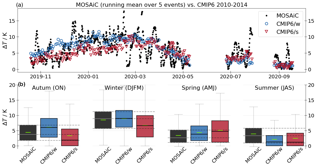
Figure 4(a) Temperature inversion strengths ΔT obtained from radio soundings during the MOSAiC expedition and for the model subsets CMIP6/w and CMIP6/s, respectively. The time series of the radio soundings during MOSAiC is given as rolling average over 10 launches. (b) Seasonal inversion strengths ΔT as box plots, corresponding to panel (a). Boxes show the 25th to 75th percentiles of the data, whiskers show the 5th to 95th percentiles, horizontal grey lines in the boxes show the median values, and horizontal green lines show the mean values. MOSAiC data were collected from October 2019 to October 2020 and are compared to co-located 6 h model data in the period of 2010–2014. Details on the data processing are given in Sect. 2.2.
3.2.1 Temperature inversions during MOSAiC
Figure 4 shows the comparison between inversion measurements during the MOSAiC expedition and co-located simulated inversion data for the CMIP6/w and CMIP6/s subsets, respectively.
The time series in Fig. 4a depicts, on average, a stronger inversion for the CMIP6/w subset during boreal autumn (ON) and extended winter (DJFM). In turn, during spring (AMJ), the CMIP6/s subset shows slightly stronger inversions, on average. For summer (JAS), both model groups have similar inversion strengths. The differences between both model subsets are most noteworthy during October to March.
We propose the following to explain the relation between the present-day inversion and historical LRF in the Arctic. The stronger inversion in CMIP6/w in the present-day period during October to March is consistent with the negative relationship between ALRF and the change in inversion strength among climate models (Boeke et al., 2021). A stronger Arctic LRF corresponds to more bottom-heavy warming in the past (i.e. a stronger depletion of the surface temperature inversion). This explains why CMIP6/s models end up having a weaker inversion in the present-day period.
During extended winter, the CMIP6/w models are in better agreement with the observations compared to the CMIP6/s subset (compare to box plots in Fig. 4b). During ON, the observations lie in between both sub-groups but are still closer to the CMIP6/w average. During AMJ, both model subsets tend to overestimate the inversion strength from the observations. However, the CMIP6/w subset is slightly closer to the observations. During JAS, both subsets show inversions that are too weak in comparison to the MOSAiC observations. However, severe data gaps during spring and summer make the interpretation somewhat less reliable.
It is noteworthy that during MOSAiC, a number of anomalous events were detected, e.g. extreme cases of warm, moist air transported from the northern North Atlantic or northwestern Siberia during late autumn until early spring (Rinke et al., 2021). That raises the question of whether MOSAiC inversion data are an appropriate choice for constraining climate models. Rinke et al. (2021) compare the near-surface meteorological conditions during MOSAiC to the context of the recent climatology and show that for the full time series, the temperature at 2 m and 850 hPa lies mostly within the record, even during storms and moisture intrusion events. We thus expect that the temperature inversion is representative of climatological averages. Another line of evidence is that the wintertime inversion during MOSAiC is similar to the wintertime inversion during the SHEBA (Surface Heat Budget of the Arctic Ocean) campaign (approx. 8 K in the averaged DJF temperature profile; Stramler et al., 2011).
In summary, from the presented comparative time series, we particularly emphasise the results presented during October to March. The R/V Polarstern drifted within the central Arctic, mostly north of 85∘ during that time (Fig. 3). CMIP6/w models simulate a stronger present-day inversion than CMIP6/s and are closer to the observed distribution during the MOSAiC expedition, primarily during winter. The model subsets during DJFM are clearly distinguishable, also by the range of individual models. The average inversion strength from those three models in the CMIP6/w and CMIP6/s subset lies within 7.6–10.6 and 5.8–6.9 K, respectively. During ON, the CMIP6/w and CMIP6/s subset results lie within 4.6–5.8 and 1.8–3.5 K, respectively. Primarily during DJFM, the MOSAiC inversion average (8.49 K) is most attributable to the range of CMIP6/w models. We further elaborate on the statistical representativeness of the results during DJFM by explicitly showing the three distributions of CMIP6/w, CMIP6/s, and the MOSAiC inversion data as a histogram in Fig. A1. It is noteworthy that the model subsets show a shift in the distribution towards lower inversion values for CMIP6/s models. We further perform a two-sample Kolmogorov–Smirnov test to compare the similarity of CMIP6/w and CMIP6/s distributions (not shown explicitly). The test indicates that both model subsets show a significantly different distribution and that this difference is largest during DJFM (also large during ON) compared to spring and summer. In addition, the highest correspondence between MOSAiC and model simulations is seen during DJFM, which is supported by Fig. A1.
Regarding the role of internal variability, we note that our conclusion that CMIP6/w models more realistically represent the MOSAiC inversion data is based on the comparison to ensemble means. However, individual CMIP6/s realisations might still be consistent with the observed inversion. Figure B1a indicates that this is not the case. The bar plots show the averaged inversion during DJFM for observed and simulated values (ensemble averages; corresponding to Fig. 4b). The grey bars further indicate the residuals after subtracting CMIP6/w and CMIP6/s averages (externally forced response) from the observations. The error bars account for internal variability in the respective model subset (see Sect. 2.9 for details). The internal variability range in the CMIP6/s model does not fully cover the MOSAiC–CMIP6/s difference. The difference can therefore not be explained with confidence by the internal variability in the CMIP6/s ensemble, as in the case for the smaller MOSAiC–CMIP6/w difference. This justifies our conclusion that CMIP6/s models systematically underestimate the inversion during DJFM. The same applies for a similar comparison during ON and AMJ (not shown).
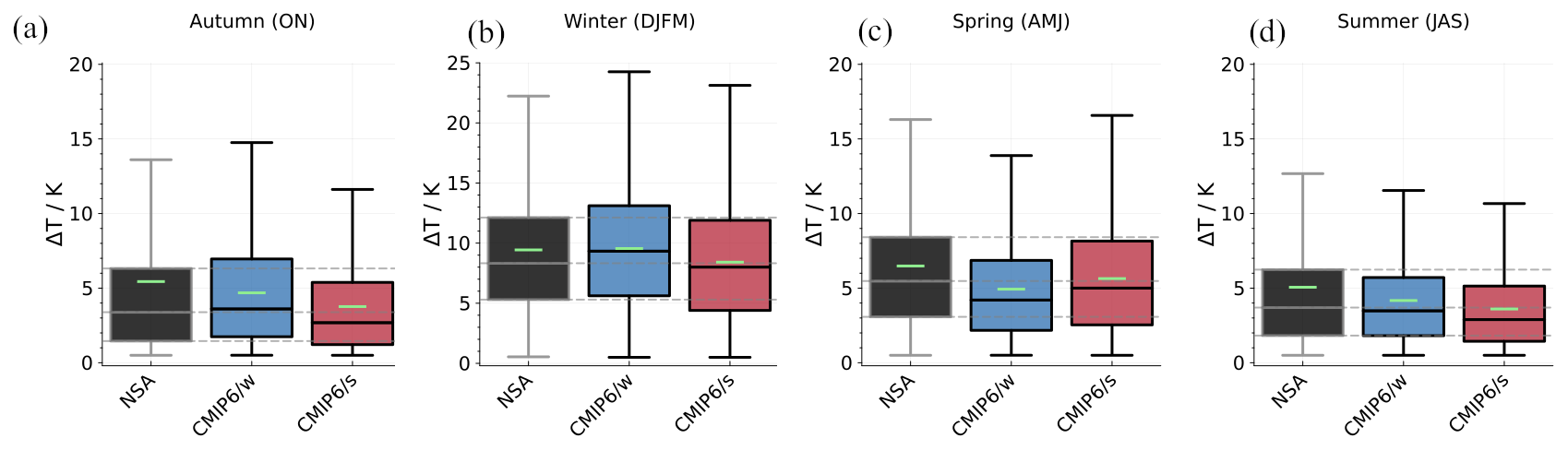
Figure 5Seasonal temperature inversion strengths ΔT as box plots, obtained from radio soundings at the NSA site, and from the model subsets CMIP6/w and CMIP6/s, respectively. The box plots correspond to Fig. 4b, showing the seasonal distribution of ΔT from radio soundings during the MOSAiC expedition. NSA data were collected during 2003–2014 and are compared to co-located 6 h model data in the period 2010–2014. Details on the data processing are given in Sect. 2.3.
3.2.2 Temperature inversions at Utqiaġvik (NSA)
The regular radiosonde observations at the Utqiaġvik site are complementary to the MOSAiC analysis in that they provide long-term statistics, although only at one site, and are representative of a different geographical (coastal) region in the Arctic. We present our results in Fig. 5 in comparison with the measurements conducted during MOSAiC. Correspondingly, the co-located model data cover the period of 2010–2014 and apply the same CMIP6 models (as defined in Table 1).
During both ON and DJFM, CMIP6/w models, on average, show a stronger inversion compared to the CMIP6/s subset, and vice versa during AMJ, which is consistent with the findings for the MOSAiC data in Fig. 4. This agreement with the findings from MOSAiC suggests that the same explanation also holds true for this longer-term analysis.
The comparison of the observed inversion data with the data from models shows that the CMIP6/w model subset lies closer to the observations in ON. For the winter case, it is somewhat less clear than for the MOSAiC comparison. The observations lie between CMIP6/w and CMIP6/s with regard to the 25th and 75th percentiles of the data. The average inversion at NSA is closer to the subset average of CMIP6/w, but the median is closer to CMIP6/s. We expect these differences, when compared to the MOSAiC analysis, to be linked to the vicinity of the ocean at the NSA site. In the following section, dropsonde measurements show that CMIP6/w models overestimate atmospheric stability over ocean, but CMIP6/s models simulate less stable conditions during the month of March. This would explain that the inversion strengths derived at NSA lie somewhere between both subsets. In addition, the model data for both subsets are less clearly distinguishable when compared to the MOSAiC sampling.
In spring, the CMIP6/w models underestimate the inversion strength when compared to the observations, while CMIP6/s models fit the observations better. This is in contrast with our MOSAiC results, which suggest that both model groups overestimate the inversion strength at this time of the year. However, due to large data gaps for MOSAiC during this season, caution should be taken when interpreting the results. During JAS, the inversion strength is underestimated in all models; this is a result that is in agreement with the MOSAiC data.
In summary, we find links between the model-to-observation comparison for the MOSAiC expedition and at the NSA site. In particular, we find that both analyses transfer from a period where the CMIP6/w model has stronger inversions (October to March) to a period where CMIP6/s models simulate more stable conditions (AMJ). Where the observations are deviating from the model average inversion strength (MOSAiC in (ON)DJFM and NSA in ON), we find that the stronger inversions, as simulated by CMIP6/w models, more realistically represent the observations. In addition, during October to March, the MOSAiC–CMIP6 (ensemble mean) difference lies within the range of internal variability for CMIP6/w but not for CMIP6/s (not shown) as seen for MOSAiC.
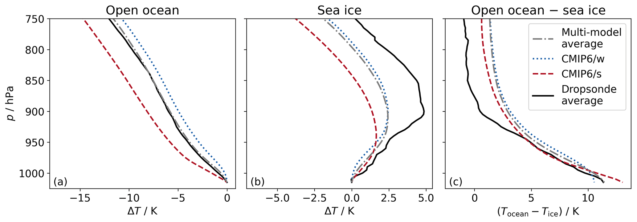
Figure 6Average profiles of temperature normalised with the temperature at 1015 hPa (ΔT) over (a) open ocean and (b) sea ice, respectively. ΔT is obtained from dropsonde launches during aircraft campaigns in the Fram Strait and the model subsets CMIP6/w and CMIP6/s, just like the model average, respectively. Seasonally, our results are restricted to the month of March. Panel (c) shows the difference between the temperature profiles over open ocean and sea ice. Dropsonde data were collected during three flight campaigns in 1993, 2013, and 2019 and are compared to co-located 6 h model data from the period of 2010–2014. Details on the data processing are given in Sect. 2.4.
3.2.3 Temperature profiles in the Fram Strait
In order to further assess the mediating effect of the surface type (open ocean or sea ice; as motivated in Fig. 2) on the temperature profile, we make use of dropsonde profiles launched from aircraft. Again, this analysis is complementary to the results from the MOSAiC and NSA data comparison and embedded in the context of local influences on the Arctic LRF. We therefore apply the same models but only include data during the end of extended winter (March), as discussed before in Sect. 2.4. The comparison with co-located CMIP6/w and CMIP6/s model subsets is shown in Fig. 6. Figure 6a and b show the temperature profiles derived from observations and models over open ocean and sea ice, respectively, which are normalised to the temperature at 1015 hPa. Note that due to a lack of open-ocean data in the CNRM-ESM2-1 (no. 25 in Table 1) domain, CMIP6/s only comprises two models.
The mean temperature profiles derived from both models and observations show an almost linear temperature decrease over open ocean, as also expected climatologically (Fig. 2a and b). In contrast, the profiles over sea ice show a near-surface temperature inversion for both the observations and the model data (in agreement with the climatological analysis in Fig. 2). Over ocean, the CMIP6/s subset shows slightly less stable conditions than the CMIP6/w data. Similarly, the CMIP6/w subset simulates a stronger inversion (on average 4.35 K), when compared to the CMIP6/s data (on average 3.55 K) over sea ice. The inversion strength is derived, as explained in previous sections, as the difference between Tmax and T2m. The stronger simulated stability in present-day temperature profiles, as projected by the CMIP6/w subset, is in agreement with previous results from MOSAiC in the central Arctic and the NSA site located near the coast during autumn and winter. Note that the difference in the stability between both subsets weakens when including campaign data from April (not shown). We attribute this to the fact that during AMJ, both MOSAiC and NSA show a transition to CMIP6/s models simulating stronger present-day inversions compared to CMIP6/w (Figs. 4 and 5, respectively). This likely leads to fewer differences between the subsets in the dropsonde data through overlapping signals between March and April. Overall, both model subsets underestimate the inversion strength compared to the observations over sea ice. However, over both open ocean and sea ice, the CMIP6/w subset is closer to the observations, although being rather consistent with the multimodel average.
To analyse the impact of sea ice retreat on the temperature profile, Fig. 6c shows the difference in profiles between open-ocean and sea ice areas. Close to the surface, the temperature difference between ocean and sea ice is larger for the CMIP6/s subset (on average 13.0 K) compared to CMIP6/w (on average 10.5 K). This is mostly due to higher near-surface air temperatures over ocean in the CMIP6/s subset (not shown). However, above 1000 hPa, the situation reverses, with a larger surface-type temperature difference for CMIP6/w models. When compared to the observations, the warming expected through sea ice retreat is slightly better depicted by the CMIP6/w models very close to the surface. However, in higher layers, the CMIP6/s models simulate a slightly more realistic temperature difference between profiles over ocean and sea ice (although the difference between models subsets is small).
We conclude that in the context of the simulated stability over sea ice, the dropsonde results representing the month of March are in agreement with the inversion data obtained from the central Arctic during MOSAiC and at the coast of the NSA site during DJFM. This concerns the stronger simulated stability by the CMIP6/w models and their closer match with observations during DJFM over sea ice, as shown by the MOSAiC observation-to-model comparison. We further show that when switching from sea ice to open ocean, the CMIP6/s models generate a stronger increase in the near-surface air temperature than the CMIP6/w models but less warming in the higher troposphere. Both results imply that there is a stronger contribution to a positive LRF embedded in the processes driving the Arctic LRF, i.e. bottom-heavy warming (BHW) and muted top-heavy warming (THW). Our data, however, are temporally limited and account solely for the month of March.
3.3 Remote aspects: atmospheric energy transport
Up to this point, we have presented results that concern the local and near-surface Arctic temperature structure and their link to the simulated past AA and Arctic LRF. We now focus on the impact of remote controls, by first extending our results shown in Fig. 6c, i.e. the evolution of bottom-heavy and top-heavy warming, and their potential to mediate the vertical warming structure in a model-to-reanalysis comparison.
3.3.1 The role of local advective heating
In this analysis on advective bottom- and top-heavy warming, we focus on the same area of the Fram Strait as in the previous section and further include the observational site of Utqiaġvik (Sect. 3.2.2). Bottom-heavy warming conceptually addresses the key feature of the Arctic LRF; i.e. the stronger warming of near-surface air masses compared to aloft. Top-heavy warming, on the contrary, describes the concept of stronger warming in the higher layers of the tropospheric column compared to the surface. To address these vertically non-uniform warming structures, we analyse the changes in the occurrence of those transport pathways that are related to either BHW or THW during extended winter (DJFM) and for the time period of interest (1985–2014 with respect to 1951–1980). Thus, we link vertically non-uniform warming structures to the large-scale circulation and further explore the potential impact on the local LRF at site. To evaluate the performance of CMIP6 models, we compare CMIP6/w and CMIP6/s model subsets to ERA5 data. The transport pathways are characterised in terms of the preferred atmospheric circulation regimes, and the warming profiles are described in terms of T2m and T500 anomalies (see Sect. 2.5 for details).
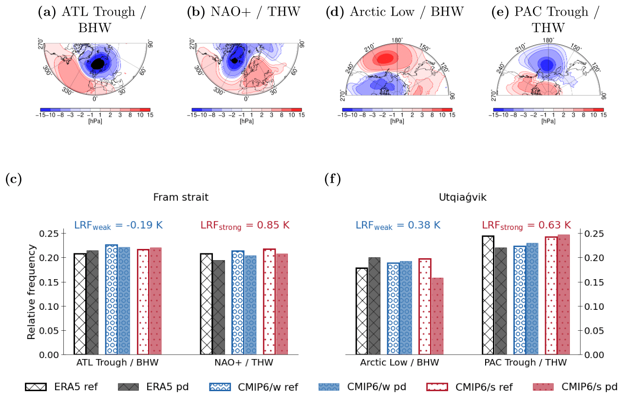
Figure 7Changes in the relative frequency of circulation regimes associated with either bottom-heavy warming (BHW) or top-heavy warming (THW) for ERA5 and the model subsets CMIP6/w and CMIP6/s, respectively. The left-hand side of the plot refers to the North Atlantic–Eurasian region (a–c) and the right-hand side to the North Pacific region (d–f). Upper rows show the circulation regimes, and lower rows show the frequency of occurrence for the reference (ref) and present-day (pd) period, respectively. Seasonally, we focus on the extended winter period DJFM. For the North Atlantic–Eurasian region, we show the SLP anomaly patterns of the two circulation regimes which are related to the (a) strong BHW (Atlantic trough or ATL Trough) and (b) strong THW (NAO+), based on ERA5 daily mean SLP data for 1979–2020. (c) Changes in the relative frequency of occurrence between the reference and the present-day period of the respective regimes over the Fram Strait. For the North Pacific region, panels (d–e) are the same as panels (a–b). The SLP anomaly patterns of the two circulation regimes, which are related to (d) strong BHW (Arctic low) and (e) strong THW (Pacific trough or PAC Trough), are based on ERA5 daily mean SLP data for 1979–2020. Panel (f) is the same as panel (c). Changes in the relative frequency between the reference period and present-day period of the respective regimes are shown, except for Utqiaġvik. The reference and present-day period in ERA5 (CMIP6) is 1979–1999 (1951–1980) and 2000–2020 (1985–2014), respectively. The values above panels (c, f) give the local LRF for CMIP6/w (LRFweak) and CMIP6/s (LRFstrong) over both domains, respectively. We use daily output data for both ERA5 and CMIP6 in this analysis. Details on the data processing are given in Sect. 2.5.
The transport pathways over the Fram Strait region (77.4–82∘ N, 0–10∘ E; see Fig. 3) are characterised by the five distinct circulation regimes over the North Atlantic–Eurasian region (e.g. Crasemann et al., 2017), namely the Scandinavian–Ural blocking regime (SCAN/Ural), the negative phase of the North Atlantic Oscillation (NAO−), the dipole pattern regime (DIPOL), the Atlantic trough regime (ATL Trough), and the positive phase of the North Atlantic Oscillation (NAO+). The application of the MNLR approach described in Sect. 2.5 reveals a high-occurrence probability of the ATL Trough regime for BHW over the Fram Strait for ERA5 (Fig. 7a) and for the climate models (not shown). The occurrence of strong THW over the Fram Strait is associated with a high probability of the NAO+ circulation regime (Fig. 7b). For ERA5, Fig. 7c shows that the ATL Trough regime (associated with BHW) occurs more frequently, and the NAO+ regime (associated with THW) occurs less frequently in the present-day period compared to the reference. Although non-significant, both of these changes imply a potentially positive feedback contribution of advection to the Arctic LRF. For the CMIP6/w models, both the ATL Trough and the NAO+ regime occur less frequently in the present-day period, with the implication of there being counteractive effects on the local LRF by advection. On the other hand, for the CMIP6/s models, the ATL Trough regime occurrence increases and the NAO+ regime occurrence decreases in the present-day period. We suggest that the differences in the sign of occurrence changes in the ATL Trough and BHW regime are related to the differences in the strength of the LRF at site when comparing the two model subsets over the Fram Strait region (discussed later on).
The transport pathways over the Utqiaġvik region (70.6–71.8∘ N, 200–205.9∘ E; see Fig. 3) are characterised by five distinct circulation regimes over the North Pacific region (e.g. Amini and Straus, 2019), namely the Pacific trough (PAC Trough), the Arctic high, the Pacific wave train, the Arctic low, and the Alaskan Ridge regime. By applying the MNLR approach, a high-occurrence probability of the Arctic low regime for BHW for ERA5 (Fig. 7d) and for the climate models (not shown) has been detected. The occurrence of THW over the Utqiaġvik region is related to a high probability of the PAC Trough regime (Fig. 7e). For ERA5, Fig. 7f shows that the Arctic low regime (associated with BHW) occurs more frequently, and the PAC Trough regime (associated with THW) less frequently in the present-day period. Again, both of these changes in the remote influences (which, at Utqiaġvik, have passed the bootstrap significance test described in Sect. 2.5) can positively contribute to the Arctic LRF. For the CMIP6/w models, both the occurrence of the Arctic low regime and the PAC Trough regime increases slightly in the present-day period, with the implication being that there are counteracting effects of advection on the local LRF. For the CMIP6/s models, the Arctic low regime occurrence decreases and the PAC Trough regime occurrence increases in the present-day period, which potentially contributes to a weakening of the positive LRF through advection over the Utqiaġvik region. In summary, at both sites of the Fram Strait and Utqiaġvik, theCMIP6/w and CMIP6/s model subsets differ from each other in terms of their changes in the relative frequency of the BHW regimes in the present-day period 1985–2014 (with respect to 1951–1980). In the Fram Strait domain, CMIP6/w models show a decrease in the relative frequency in BHW, while CMIP6/s models show an increase. Both have less THW in the present-day period. Thus, we suggest a negative LRF contribution to CMIP6/w and a positive LRF contribution to CMIP6/s models through the influence of advective BHW in the Fram Strait, respectively. At Utqiaġvik, the situation is reversed. CMIP6/w models show an increase in the relative frequency in BHW, while CMIP6/s models show a decrease. Both have more THW in the present-day period. Thus, we suggest a positive LRF contribution to CMIP6/w and a negative LRF contribution to CMIP6/s models through the influence of advective BHW at Utqiaġvik, respectively. We link these differences between the model subsets at both locations to the magnitude of the co-located LRF (values given in Fig. 7c and f) later on in the discussion.
In terms of their similarities with ERA5 results, the changes in advective BHW and THW show that the CMIP6/s models have a closer resemblance to ERA5 over the Fram Strait. At Utqiaġvik, the ERA5 data, however, show an opposite tendency in the evolution of BHW and THW in comparison with CMIP6/s models. For the CMIP6/w models, only the increase in BHW is consistent with ERA5, although less pronounced in the models. Note that by applying the bootstrap test, we determine significant changes at the 95 % level only at the site of Utqiaġvik (for changes in BHW and THW in ERA5 and in BHW for CMIP6/s models). Although the attribution of model-simulated results to reanalyses remains somewhat illusive, we argue that the differences in the change in occurrence of BHW and its link to the local LRF at the site motivates a more extensive investigation of the link between large-scale circulation regimes that impact the evolution of local vertical warming structures and local differences in Arctic temperature feedbacks.
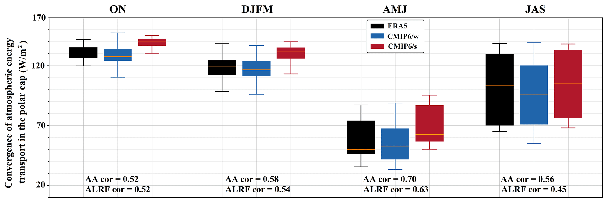
Figure 8Seasonal pan-Arctic atmospheric energy transport convergence north of 66∘ N, obtained from ERA5, and the model subsets CMIP6/w and CMIP6/s, respectively, during 2000–2014. The seasonal inter-model correlation coefficients between the seasonal mean of the transport term and historical AA and ALRF (including all models in Table 1) are given in the lower part of each panel. We use monthly output data for both ERA5 and CMIP6 in this analysis. Details on the derivation of atmospheric energy transport convergence are given in Sect. 2.6.
3.3.2 Pan-Arctic atmospheric energy transport convergence
In the second step of the consideration of remote controls on the Arctic LRF, we extend the perspective of energy transport to a broader view. Figure 8 depicts the total poleward atmospheric energy transport convergence within the Arctic boundary during each season for ERA5, CMIP6/w, and CMIP6/s subsets, respectively. The present-day transport accounts for the averaged period of 2000–2014 for both CMIP6 and reanalysis data. First, it is shown that deriving the atmospheric energy transport convergence as the residual of the energy budget equation (see Sect. 2.6 for details) gives a realistic approximation of the seasonal cycle of the Arctic energy transport. During late autumn and winter, the atmospheric energy transport convergence into the polar cap shows a seasonal maximum due to the absence of solar irradiance. The Arctic atmosphere is in an approximate balance between long-wave radiative cooling and the advection of energy from lower latitudes (Cronin and Jansen, 2016). During spring and early summer, the long-wave cooling intensifies due to higher atmospheric temperatures, but the incoming solar radiation adds a heat source to the atmosphere, which leads to a decrease in the seasonal atmospheric transport into the polar cap (e.g. Trenberth, 1997; Serreze et al., 2007; Linke and Quaas, 2022).
From the differences between the CMIP6/w and CMIP6/s simulations, it is shown that the present-day poleward transport convergence is stronger for the CMIP6/s subset when compared to the CMIP6/w models. This is true for each season, and furthermore, the difference appears to be systematic across the entire model ensemble. The transport convergence and AA and ALRF are positively correlated across all models, which is shown by the inter-model correlation coefficients in the lower part of Fig. 8. This correlation (cor) is particularly strong during AMJ, with AA cor = 0.70 and ALRF cor = 0.63, but it is always above 0.5 (except for ALRF cor during JAS). In addition, the seasonal inter-model mean correlation of the transport term with both AA and ALRF is statically significant throughout the year when using the bootstrapped method with a 0.95 confidence level (see Sect. 2.6 for details). We therefore conclude that the model differences in a simulated atmospheric energy transport convergence are systematic in that stronger AA and ALRF models show a stronger present-day transport, and vice versa for weaker AA and ALRF models.
To evaluate which of the model subsets more realistically projects the atmospheric transport into the polar cap, we compare both CMIP6/w and CMIP6/s simulations to ERA5 results. The box plots in Fig. 8 show that the reanalyses is closer to the transport as simulated by CMIP6/w models during October to March. During AMJ, the ERA5 transport convergence lies between both CMIP6/w and CMIP6/s subsets in terms of its distribution but is slightly closer to CMIP6/w. During JAS, the box plot in Fig. 8 implies that CMIP6/s models more realistically simulated the atmospheric transport convergence into the polar cap.
In summary, we find that during each season, models with weaker (stronger) present-day poleward transport convergence simulate a smaller (larger) past AA and ALRF with statistical significance. For the model-to-reanalyses comparison, we find that during October to March, CMIP6/w models with lower present-day transport convergence more realistically to resemble ERA5 results. During JAS, CMIP6/s models more realistically resemble the transport estimate of ERA5, but the model differences, and thus their attribution to reanalyses, are less clear when compared to October to March.
We further show, in Fig.B1b, that during DJFM, the difference between the average transport in ERA5 and CMIP6/w (ensemble mean) can be mostly explained by the simulated internal variability within the CMIP6/w subset, although not fully. However, due to the positive correlation between AA and ALRF and transport convergence (r=0.58 and r=0.54, respectively), the difference is reduced when choosing, for example, the three next-highest models for CMIP6/w, which is then covered by the simulated internal variability range (not shown). We thus conclude that CMIP6/s models more likely overestimate the energy transport convergence.
Last, we find similarities in previous model-to-observation comparisons of the thermal structure of the lower boundary layer. Our results in Sect. 3.2 have shown that during autumn and extended winter, but primarily during DJFM, the CMIP6/w models more realistically resemble observations of the surface-based temperature inversion over sea ice. We find now that also in the representation of processes that can further affect the free troposphere (energy transport from lower latitudes), CMIP6/w models are closer to reanalyses, primarily during DJFM.
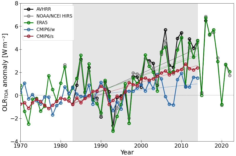
Figure 9Time series of the OLRTOA anomaly with respect to 1983–1997 for AVHRR, NOAA and NCEI HIRS, and ERA5 climate data records (averaged to provide a best combined record of OLR data; BEST COMB), just like the model subsets CMIP6/w and CMIP6/s, respectively. Trends are derived for both satellite observations and reanalyses and model subsets in the form of the linear fit for the data overlap period (1983–2014; shaded area). The trends are 0.138 ± 0.017, 0.037 ± 0.010, and 0.106 ± 0.009 for BEST COMB, CMIP6/w, and CMIP6/s, respectively. The uncertainty ranges account for the standard deviation of the trends, using the bootstrap method of Lelli et al. (2023). The fluxes are averaged over the Arctic area north of 66∘ N and account for the extended winter period DJFM. From CMIP6, we use the collection of monthly mean model diagnostics. Details on the data processing are given in Sect. 2.7.
3.4 Pan-Arctic outgoing long-wave radiation at the TOA
As introduced earlier, the global LRF builds on either the limited atmospheric cooling in the long-wave spectrum (like in the Arctic) or an intensification of this process (i.e. a reduced greenhouse effect, as seen in the tropics) when compared to vertically uniform warming. Thus, the LRF (amongst other feedbacks and forcings) mediates changes in the TOA energy budget. In our final step, we investigate changes in the outgoing long-wave radiation at the TOA during the past few decades. Within the scope of the TOA energy budget, we seek to constrain the overall LRF in the Arctic by a model-to-satellite or reanalysis comparison, covering the period of 1983–2014 (from the beginning of the full-year satellite record to the end of the CMIP6 simulations). Due to previous links found between the intermediate conclusions in Sect. 3.2 and 3.3, we focus on the most relevant winter season (DJFM).
Figure 9 depicts an overall increases in OLRTOA within the period of interest, which is consistent with atmospheric warming. The CMIP6/s subset shows a stronger increase in OLRTOA compared to CMIP6/w, which coincides with a notoriously stronger warming in the CMIP6/s simulations (not shown).
Looking at the anomaly in OLRTOA with respect to 1983–1997, the BEST COMB trend (average of AVHRR, NOAA and NCEI HIRS, and ERA5 records) shows a stronger increase in OLRTOA (0.138 ± 0.017 ) when compared to both CMIP6/w and CMIP6/s subsets (with an increase of 0.037 ± 0.010 and 0.106 ± 0.009 , respectively). Overall, the CMIP6/s subset is closer to the BEST COMB trend but still underestimates the increase in OLRTOA. In a TOA perspective, both model subsets underrepresent the change in the increasing OLRTOA with advanced global warming. This links to a general inability of climate models to project the magnitude of Arctic climate change during the most recent decades (discussed later on).
Including the aspect of internal climate variability, Fig. B1c indicates a large spread across individual realisations for both model subsets (error bars). The conclusion that CMIP6/s simulations more realistically represent the observed OLRTOA trends is supported by the smaller difference between BEST COMB and CMIP6/s when compared to CMIP6/w. This difference lies within the range of internal variability (as simulated by CMIP6/s). On the other hand, the difference between BEST COMB and CMIP6/w cannot be fully explained by the range of internal variability simulated by the CMIP6/w models, which justifies the conclusion that CMIP6/w models systematically underestimate the OLRTOA trend.
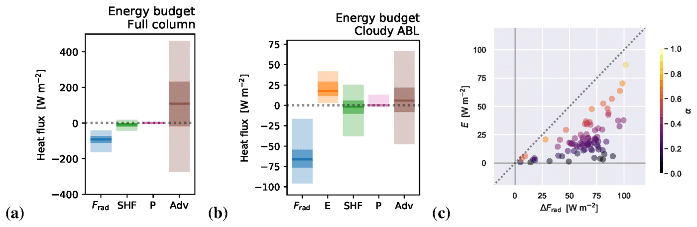
Figure 10LES results for the MOSAiC drift. (a) Drift-averaged heat budget of the full atmospheric column. (b) Conditionally averaged atmospheric boundary layer (ABL) heat budget for all days with a non-zero liquid water path (83 out of 300 simulated days). Budget terms include the net radiative heating (Frad), top entrainment heat flux (E), surface sensible heat flux (SHF), surface precipitation in any form (P), and vertically integrated large-scale advection (Adv). Each term is shown as a distribution, with the median (thick line), interquartile range (dark shading) and 9th–95th percentile range (light shading). (c) Scatterplot of daily average long-wave cooling across the liquid cloud layer versus the entrainment heat flux at the atmospheric boundary layer inversion. Colours represent the entrainment efficiency α, as defined in the text. Details on the data processing are given in Sect. 2.8.
Up to this point, we have compared key features of the Arctic LRF and AA in the current climate to co-located model simulations with both weak and strong simulated ALRF and AA in the past. Our model-to-observation and reanalysis comparisons covered the key aspects of Arctic temperature inversion, sea ice retreat, local air mass advection, and pan-Arctic atmospheric energy transport convergence, as well as the link between AA and ALRF and changes in the TOA long-wave radiation budget with warming. On the other hand, processes at turbulence- and cloud-resolving scales are largely underrepresented in the literature covering the Arctic LRF. In our final step, we show the potential of these processes to impact the evolution of the Arctic temperature profile. We thus link to our results in Fig. 2, which motivated the role of clouds in the evolution of the Arctic temperature profile in a purely CMIP6-based analysis. The next section deepens this analysis in the scope of a local energy budget perspective in large-eddy simulations covering the MOSAiC drift. We treat this section separately from the constraint approach and thus put the comparison climate model data into a section devoted to providing an outlook perspective.
3.5 Outlook: the role of advection, clouds, and entrainment in large-eddy simulations (LES)
To gain insight in the role of clouds and boundary layer dynamics, we now investigate the Arctic energy budget in more detail, using output data from year-long LES covering the MOSAiC drift. The results are shown in Fig. 10.
Averaged over all 300 daily simulations, we find that the full column heat budget is approximately in radiative–advective equilibrium (RAE; Fig. 10a). This RAE has been previously introduced as basic-state model for representing the high-latitude atmosphere (Cronin and Jansen, 2016). Even if only a certain number of weather situations were sampled during the drift, and even if the scatter in particular in the advective heating remains large, this confirms what is expected for the large-scale energy budget of the ice-covered Arctic. In particular, the sensible heat flux (SHF) and precipitation (P; representing net condensation and freezing in the column) are negligible compared to the radiative cooling (Frad) and vertically integrated large-scale advection (Adv).
The situation is rather different when (i) only analysing cases with low-level liquid cloud mass and (ii) considering the heat budget for the atmospheric boundary layer (ABL). For the whole drift, about 1 out of 3 d feature low-level liquid clouds. This frequency of occurrence is roughly consistent with the findings of Bennartz et al. (2013) and is an expression of the resilience of mixed-phase clouds at high latitudes (Morrison et al., 2012). In contrast to the full column, the ABL heat budget shows an imbalance in which the radiative cooling dominates (Fig. 10b). On average, this leads to a gradual cooling of the ABL in cloudy cases, which likely expresses the ongoing transformation of warm and moist air masses in which these clouds are embedded (Pithan and Mauritsen, 2014; Pithan et al., 2018).
An intriguing result in the context of the LRF is the significant role played by entrainment at the top of the ABL, which is here defined as the height of the strongest gradient in liquid water potential temperature (θl) in the lowest 5 km. In these cloudy cases, in addition to the weak advective heating, the warming of the ABL due to the entrainment flux (E) is significant, while the sensible and latent heat flux are again negligible, as was the case in all-sky conditions (Fig. 10b). The entrainment heating (E=ϵtΔθl) depends on the ABL top entrainment rate (ϵt) and the temperature jump across the inversion (Δθl), which is an expression of the local (elevated) inversion strength. Entrainment warming can only counteract the radiative cooling partially, an effect which is investigated in further detail in Fig. 10c. The impact on the ABL heat budget is expressed by the entrainment efficiency (α) and defined as the ratio of entrainment warming to the radiative cooling (Stevens et al., 2005):
We find that, on the basis of these year-long LES results for the MOSAiC drift, for mixed-phase Arctic clouds, this ratio is about one-third, implying that entrainment warming is never able to fully balance the radiative cooling. However, it still significantly counteracts the gradual cooling of warm and moist air masses that enter the Arctic system. In this process, the main role of the inversion strength is to determine the entrainment warming. As a result, it modulates the transformation of such warm cloudy air masses, with the effect being that it keeps them warm for longer. This in turn affects the LRF, in particular in ice-covered areas over which such cloudy air masses travel.
We have presented data from several Arctic-based observations and reanalyses in conjunction with co-located CMIP6 model simulations to constrain various processes and relevant parameters that mediate both the Arctic amplification and the Arctic LRF. We thus exploit the considerable inter-model spread in simulated AA and ALRF, which are linearly related across CMIP6 models. For the linear relationship between AA and ALRF, we show that models with stronger positive ALRF values contribute more to AA, through locally enhancing global warming in the Arctic and cooling the tropics, which does not necessarily reflect in the inter-model spread of projected global warming.
Our process-oriented constraints attribute observable aspects of the current climate system to co-located CMIP6 simulations from models that have projected either a weak or a strong AA and ALRF in the past. This allows us to establish a link between key aspects of the current climate and the evolution of AA and ALRF in the past. The magnitude of ALRF and AA for the historical past is defined as the time period of 1951–2014.
For our constraint, we first make use of the hypothesis that AA and ALRF are related to the lack of boundary layer mixing in the Arctic. Previous literature, since the earliest global dynamical simulations of climate change, has demonstrated that stable stratification is a necessary condition for a positive LRF in the Arctic (Manabe and Wetherald, 1975). This leads to the hypothesis that the ALRF inter-model spread is correlated to the change in the inversion strength, which is associated with bottom-heavy warming (Boeke et al., 2021; Feldl et al., 2020). Another hypothesis suggests that a stronger initial stratification produces a more positive feedback, without there being a consensus among scientists. Here, we look at present-day, surface-based temperature inversion data in the scope of a model-to-observation comparison. We use two data sets of radiosondes launched during the MOSAiC expedition in the central Arctic and from the permanent ARM site at Utqiaġvik (NSA). Using dropsonde observations from research aircraft during several boreal springtime campaigns, we quantify the contrast in the temperature profiles over sea ice and the open ocean in the Fram Strait. We aim to constrain the impact of sea ice retreat, which is widely considered to be a strong source of bottom-heavy warming over the Arctic ocean.
In spite of their spatiotemporal differences in data acquisition, we find distinct similarities in the individual comparisons of MOSAiC, NSA, and dropsonde data when compared to CMIP6. Our results confirm that during the autumn and extended winter (October to March), models that simulated a weaker AA and ALRF in the past have stronger inversions over sea ice in the present. We argue that during the autumn and winter, a key feature of the positive Arctic LRF, bottom-heavy warming has led to a stronger depletion of the surface-based temperature inversion in those models that had stronger AA and ALRF since 1951–1980. Based on the CMIP6 comparison to dropsonde data, we show that even though CMIP6/s models simulate weaker present-day inversions (consistent with MOSAiC and NSA), the sea ice melt remains an important process to mediate a stronger bottom-heavy warming and, by extension, positive LRF in future scenarios when compared to CMIP6/w models. In sum, all model-to-observation comparisons suggest an overall more realistic depiction of the lower thermal structure of the boundary layer over sea ice by models that had weak simulated AA and ALRF in the past during October to March. On the other hand, the residual between the observations and CMIP6/s simulations suggests that these models systematically underestimate the temperature inversion, rather than being a manifestation of simulated internal variability.
We want to emphasise that interpreting the local and near-surface thermal structure up to this point relies on a small number of models (see Table 1) that provide the required time resolution for a comparison of the inversion data. Therefore, our analysis is limited by data availability. For model comparisons with MOSAiC (just like NSA and dropsonde) data, we use model averages from models 5, 6, and 10 to derive CMIP6/w and models 25, 28, and 29 for CMIP6/s simulations, respectively. In particular, the CMIP6/w subset does not represent the lower edge of the simulated AA range across all used CMIP6 models (see Fig. 1b). However, the classification into a weak and strong AA model subset is still justified by the fact that the CMIP6/w and CMIP6/s AA averages lie below and above the OBS estimate of past AA values, respectively. We further tested the sensitivity of the model-to-observation comparison to the number of models chosen for the CMIP6/w and CMIP6/s classification in this time resolution group. Therefore, we added the next-highest or next-lowest AA model to the CMIP6/w and CMIP6/s subset (model 11 and 21), respectively. This addition of the models has no qualitative effect on our key conclusions that CMIP6/w models show stronger inversions during October to March and are overall closer to the observations than CMIP6/s. We further emphasise that, although the statistical interpretation due to the lack of data remains vague, the combined comparison of radiosonde data during MOSAiC and at the NSA site, just like the dropsonde data from flight campaigns in the Fram strait, agree with respect to the main emerging points discussed above.
On the other hand, not only local processes but also remote influences like the poleward atmospheric energy transport have the potential to mediate the ALRF and AA. First, we consider the impact of advective bottom- and top-heavy warming on the local LRF, which is connected to changes in typical circulation regimes. The hypothesis is that an increased frequency of occurrence of weather situations favouring BHW imposes a positive contribution on the LRF. In turn, more frequent events of THW aid long-wave cooling in higher layers, thus weakening the positive LRF. We focus on the period of extended winter (DJFM) in our analysis and, locally, on the observational sites of Utqiaġvik and the Fram Strait. At the two measuring sites, the CMIP6/w and CMIP6/s models differ from each other in terms of their change in the relative frequency of BHW regimes ongoing from 1951. We suggest a link between the change in the advective BHW and LRF at site. Our data show that in the Fram Strait, the difference in LRF between CMIP6/w (−0.19 K) and CMIP6/s (0.85 K) is larger when compared to Utqiaġvik, where the difference in LRF between CMIP6/w (0.38 K) and CMIP6/s (0.63 K) is smaller by a factor 4. We relate this to an increase (decrease) in BHW in CMIP6/s (CMIP6/w) in the Fram Strait region, where we hence expect an even bigger spread in the local LRF between both model subsets and a decrease (increase) in BHW in CMIP6/s (CMIP6/w) at the site in Utqiaġvik, where we also expect a reduction in the spread in the local LRF between both model subsets. In short, the advective BHW increases the climatological spread between CMIP6/w and CMIP6/s simulated LRF in the Fram Strait and decreases it at Utqiaġvik. Although we cannot exclude the possibility that these differences are also linked to local factors (e.g. sea ice reduction) between the two simulations, our results hint at a signature of advective influences mediating the spatial pattern of the Arctic LRF. Although no conclusive results are found in the attribution of either CMIP6/w or CMIP6/s model simulations to ERA5 results, we want to highlight the potential of linking local differences in the model-projected magnitude of the LRF to changes in vertically non-uniform warming structures that are mediated by changes in the large-scale circulation.
While we present our previous results as a detailed analysis of the vertically resolved temperature change and local feedback aspects, we further extend this perspective to speculate on the coupling between pan-Arctic atmospheric energy transport (convergence) and past AA and ALRF. Our results show that a stronger present-day transport convergence within the Arctic boundary is systematically related to a stronger annual mean AA and ALRF in the past. It is useful to consider the energetic framework for explaining the positive relationship between present-day atmospheric transport convergence and AA. We specifically show, in an analysis of OLR at the TOA, that CMIP6/s models have a stronger cooling tendency in terms of OLRTOA. It is likely that the stronger cooling at the TOA due to more advanced Arctic warming in these simulations requires a larger overall atmospheric transport convergence into the polar cap to balance the radiative cooling and ensure the local energy budget (Linke and Quaas, 2022). To constrain the remote aspects of the current climate, we show that CMIP6/w models overall resemble the ERA5 transport term more realistically during October to March. On the other hand, the overestimation of the energy transport convergence in the CMIP6/s model subset cannot be explained fully by the simulated internal variability.
To finalise the constraint of past AA and ALRF, we compare recent trends of OLR at the TOA to observational estimates. The CMIP6-derived OLRTOA trends of the past 30–40 years underestimate the observations. Recent work by Rantanen et al. (2022) shows that since 1979, the Arctic has warmed more drastically than previously thought and that CMIP6 models underrepresent the warming trend that is depicted by observations. We see a link to these results when exploring the trend in OLR that has occurred at the TOA since 1983 during DJFM. Both CMIP6/w and CMIP6/s models show lower trends in the increasing OLRTOA when compared to the observations. However, for CMIP6/s models, this underestimation of the OLR trend can be interpreted as a manifestation of simulated internal variability.
To motivate a deeper perspective on clouds, boundary layer dynamics, and advective heating at the process level, we conduct a large sample of small-domain daily LES complementing the MOSAiC full drift. Averaged over all cases, the radiative cooling of the full atmospheric column is balanced by advective heating (through RAE). However, for liquid-bearing cloudy boundary layers, the entrainment heating of the boundary layer is significant, and even more important than horizontal advection, despite only modest efficiencies in counteracting the radiative cooling. This links to Fig. 2c, which implies a negative contribution of clouds to the LRF in the lower ABL (extending up to 850 hPa) but a positive contribution in higher layers. We draw two conclusions from this result. First, entrainment heating represents a significant internal column redistribution of heat, which impacts the lapse rate over sea ice. Second, liquid-bearing cloudy boundary layers are not in strict RAE but are closer to a radiative–convective–advective equilibrium due to the significance of the top-down convective heating through entrainment. However, full equilibrium is not reached, indicating that these liquid-bearing, low-level air masses are still in the process of cooling. How these low-level processes in effect contribute to AA and the ALRF requires further research, for example, by conducting LES for perturbed climate conditions.
Beyond the processes analysed in the present study, the rate at which sea ice melted in the study period also plays a large role for simulated AA and ALRF. However, we do not find a strong relation between skill levels in simulating sea ice and its decline and the magnitude of AA within a model. CMIP6 models that are identified as being capable of simulating a realistic volume of sea ice loss together with a plausible change in global mean temperature over time (1979–2014; Notz and the SIMIP Community, 2020) span across our collection of models (acronyms in bold in Table 1).
We have presented a variety of Arctic-based observations and reanalyses, in conjunction with projections of state-of-the art climate models, within CMIP6 to find synergy among them in support of advancing our understanding of AA and the Arctic LRF. We propose a constraint on past AA and ALRF by attributing observable aspects of the current climate system to co-located CMIP6 simulations by models that have projected either a weak or a strong AA and ALRF during the past few decades. In the scope of our main hypotheses formulated in points 1–3 of the introduction, we conclude the following key results, which largely focus on seasonal results during boreal autumn and winter:
-
Our data sets for boreal winter (and autumn) show that the vertical temperature structure of the Arctic boundary layer is more realistically depicted in climate models with weak simulated AA and ALRF in the past. The attribution of observations to CMIP6/w models during DJFM is mainly based on data collected during the MOSAiC expedition (representing the central Arctic during that time) and dropsonde measurements in the Fram strait over sea ice. The CMIP6/w models in particular simulate a stronger present-day temperature inversion through less depletion in the past and generate a smaller low-level warming through sea ice retreat. The latter implies that ,for CMIP6/w models, there is less warming close to the surface for a given volume of sea ice retreat and thus a smaller contribution to the positive ALRF through this process. More specifically, CMIP6/w models remain CMIP6/w models in future scenarios in this context.
-
An analysis of the pan-Arctic atmospheric transport convergence within the polar cap supports these constraints and means that this remote aspect that can further mediate the warming structure in the free troposphere is more realistically represented by climate models with weak simulated AA and ALRF in the past during autumn and winter. In particular, CMIP6/w models systematically simulate a smaller present-day atmospheric energy transport convergence in the Arctic during boreal autumn and winter, which is consistent with reanalyses. We further explore changes in the leading transport pathways that mediate vertically non-uniform warming structures, namely bottom- and top-heavy warming. Although no clear attribution of either CMIP6/w or CMIP6/s models to reanalysis results is possible, we highlight the potential of establishing links between large-scale regulated vertical warming structures and the spatial distribution of Arctic feedbacks.
-
Last, we show the difference in temperature profiles and surface energy budget between cloudy and clear-sky conditions in CMIP6 models and LES data, respectively. Both climate models and LES simulations show that in cloudy cases, the vertical mixing becomes an important heating term for the boundary layer. Even though we do not engage in a deeper study to attribute the representation of these processes to either weak or strong AA and ALRF simulations in the past, we want to motivate a perspective on the role of clouds on boundary layer dynamics and vertical warming structures. These processes are notoriously underrepresented in the literature concerning the Arctic LRF, but both the local energy budget and vertical heat distribution can play an important role in its evolution.
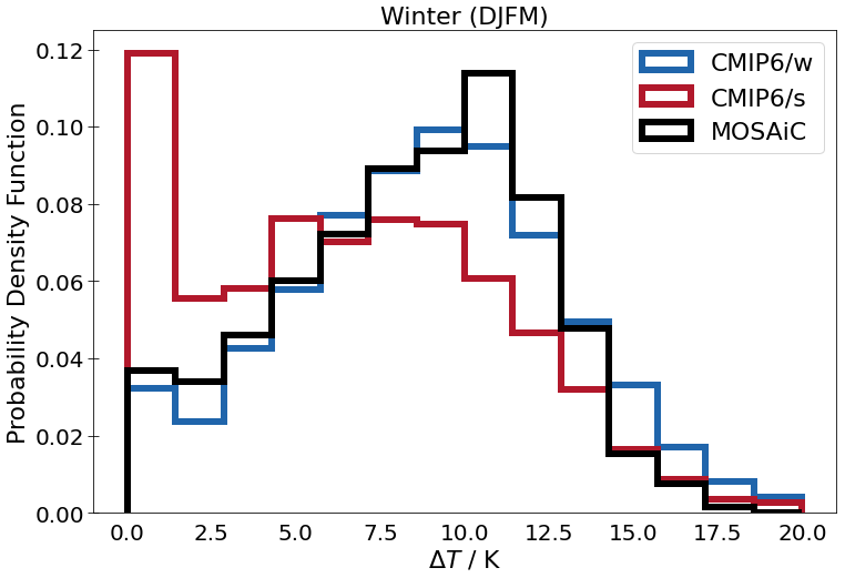
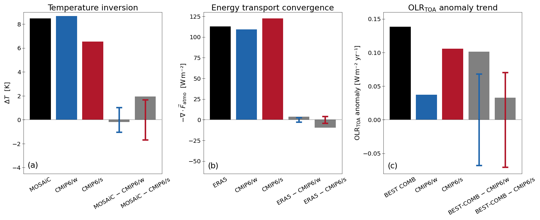
Figure B1The role of internal variability. (a) Averaged temperature inversion during DJFM for MOSAiC (black) and co-located CMIP6/w (blue) and CMIP6/s (red) model data. Model data are expressed as ensemble means over all available realisations per subset. Grey bars give the residuals after subtracting the externally forced simulations (CMIP6/w and CMIP6/s ensemble means) from the observed inversion. The error bars indicate the 95 % range of simulated internal variability for both CMIP6/w (blue) and CMIP6/s (red) models, respectively. Each year of the present-day model period is considered separately for the derivation of the range to estimate the simulated internal variability. Panels (b,)̧ are analogous to panel (a) but for comparing observations and reanalyses of atmospheric energy transport convergence and OLRTOA anomaly trends to co-located CMIP6 data, respectively.
The LES code (DALES) used in this study is open-access and available on GitHub at https://github.com/dalesteam/dales (Heus et al., 2010). The current version of DALES (https://doi.org/10.5281/zenodo.5642477, van Heerwaarden et al., 2021; dales 4.3, with an extension for mixed-phase microphysics) is available on GitHub at https://github.com/jchylik/dales/releases/tag/dales4.3sb3cgn (last access: 8 November 2021).
CMIP6 data were provided by the DKRZ (Deutsches Klimarechenzentrum; https://esgf-data.dkrz.de/search/cmip6-dkrz/, last access: 27 March 2023; see Table 1 for further information). GISTEMP data are available from https://data.giss.nasa.gov/gistemp/ (GISTEMP Team, 2023), Berkeley Earth data are from http://doi.org/10.5281/zenodo.3634713 (Rohde and Hausfather, 2019), HadCRUT5 data are from https://www.metoffice.gov.uk/hadobs/hadcrut5/data/current/download.html (Morice et al., 2021), and NOAA data are from https://doi.org/10.25921/9qth-2p70 (Zhang et al., 2019). Data from radiosondes launched during the MOSAiC expedition can be downloaded from PANGAEA (https://doi.org/10.1594/PANGAEA.928656, Maturilli et al., 2021). Near-surface temperature data during MOSAiC can be downloaded from the Arctic Data Centre (https://doi.org/10.18739/A2VM42Z5F, Cox et al., 2021). NSA radiosonde data are available from the DOE ARM data repository (https://doi.org/10.5439/1095316, Jensen et al., 1998). Dropsonde data from the three different aircraft campaigns considered in our study can be downloaded from the PANGAEA repository (Lüpkes and Schlünzen, 1996, https://doi.org/10.1594/PANGAEA.857807; Lüpkes et al., 2021, https://doi.org/10.1594/PANGAEA.936635; Becker et al., 2020, https://doi.org/10.1594/PANGAEA.921996). ERA5 data can be downloaded from the ECMWF data catalogue at https://doi.org/10.24381/cds.f17050d7 (Hersbach et al., 2023). AVHRR OLR data are available at the DWD website (https://doi.org/10.5676/DWD/ESA_Cloud_cci/AVHRR-PM/V003, Stengel et al., 2019). NOAA and NCEI HIRS OLR data can be downloaded at https://doi.org/10.24381/cds.85a8f66e (Hai-Tien and NOAA CDR Program, 2018).
The study was conceived by OL and JQ, with contributions by all authors. OL performed the CMIP6 model analyses and many of the model-to-observation or reanalysis comparisons. CS contributed the feedback analysis tools and advised on their application and interpretation. BV and OL analysed the MOSAiC data vs. CMIP models, with substantial help from MDS and SD. The Utqiaġvik analysis was carried out by PSG, FB, and HKL, together with OL. SB, AE, and MW contributed the dropsonde analysis, together with OL. The analysis on local advection and circulation patterns was provided by DH, with input from OL. The pan-Arctic energy transport analysis was contributed by SM and CJ, with support by OL. RN, JC, and NS performed and analysed the LES. MV, LL, and KV analysed the satellite retrievals. GS advised on the role of sea ice. All authors contributed to writing the paper.
At least one of the (co-)authors is a member of the editorial board of Atmospheric Chemistry and Physics. The peer-review process was guided by an independent editor, and the authors also have no other competing interests to declare.
Publisher's note: Copernicus Publications remains neutral with regard to jurisdictional claims in published maps and institutional affiliations.
We gratefully acknowledge the funding by the Deutsche Forschungsgemeinschaft (DFG, German Research Foundation; grant no. 268020496 – TRR 172) within the Transregional Collaborative Research Centre “ArctiC Amplification: Climate-Relevant Atmospheric and SurfaCe Processes and Feedback Mechanisms (AC)3”. Matthew D. Shupe has been supported by a Mercator Fellowship as part of (AC)3. The authors would like to thank Benjamin Kirbus for constructive comments on the paper.
This research has been supported by the Deutsche Forschungsgemeinschaft (grant no. 268020496).
This paper was edited by Hailong Wang and reviewed by two anonymous referees.
Amini, S. and Straus, D. M.: Control of storminess over the Pacific and North America by circulation regimes, Clim. Dynam., 52, 4749–4770, https://doi.org/10.1007/s00382-018-4409-7, 2019. a
Becker, S., Ehrlich, A., Stapf, J., Lüpkes, C., Mech, M., Crewell, S., and Wendisch, M.: Meteorological measurements by dropsondes released from POLAR 5 during AFLUX 2019, PANGAEA – Data Publisher for Earth & Environmental Science [data set], https://doi.org/10.1594/PANGAEA.921996, 2020. a, b
Bennartz, R., Shupe, M. D., Turner, D. D., Walden, V. P., Steffen, K., Cox, C. J., Kulie, M. S., Miller, N. B., and Pettersen, C.: July 2012 Greenland melt extent enhanced by low-level liquid clouds, Nature, 496, 83–86, https://doi.org/10.1038/nature12002, 2013. a
Bentsen, M., Oliviè, D. J. L., Seland, y., Toniazzo, T., Gjermundsen, A., Graff, L. S., Debernard, J. B., Gupta, A. K., He, Y., Kirkevåg, A., Schwinger, J., Tjiputra, J., Aas, K. S., Bethke, I., Fan, Y., Griesfeller, J., Grini, A., Guo, C., Ilicak, M., Karset, I. H. H., Landgren, O. A., Liakka, J., Moseid, K. O., Nummelin, A., Spensberger, C., Tang, H., Zhang, Z., Heinze, C., Iversen, T., and Schulz, M.: NCC NorESM2-MM model output prepared for CMIP6 CMIP, Earth System Grid Federation [data set], https://doi.org/10.22033/ESGF/CMIP6.506, 2019. a
Block, K., Schneider, F. A., Mülmenstädt, J., Salzmann, M., and Quaas, J.: Climate models disagree on the sign of total radiative feedback in the Arctic, Tellus A, 72, 1–14, https://doi.org/10.1080/16000870.2019.1696139, 2020. a, b
Boeke, R. C., Taylor, P. C., and Sejas, S. A.: On the Nature of the Arctic's Positive Lapse-Rate Feedback, Geophys. Res. Lett., 48, e2020GL091109, https://doi.org/10.1029/2020GL091109, 2021. a, b, c, d, e, f
Boucher, O., Denvil, S., Levavasseur, G., Cozic, A., Caubel, A., Foujols, M.-A., Meurdesoif, Y., Cadule, P., Devilliers, M., Ghattas, J., Lebas, N., Lurton, T., Mellul, L., Musat, I., Mignot, J., and Cheruy, F.: IPSL IPSL-CM6A-LR model output prepared for CMIP6 CMIP, Earth System Grid Federation [data set], https://doi.org/10.22033/ESGF/CMIP6.1534, 2018. a
Cao, J. and Wang, B.: NUIST NESMv3 model output prepared for CMIP6 CMIP, Earth System Grid Federation [data set], https://doi.org/10.22033/ESGF/CMIP6.2021, 2019. a
Cohen, J., Screen, J. A., Furtado, J. C., Barlow, M., Whittleston, D., Coumou, D., Francis, J., Dethloff, K., Entekhabi, D., Overland, J., and Jones, J.: Recent Arctic amplification and extreme mid-latitude weather, Nat. Geosci., 7, 627–637, 2014. a
Cox, C., Gallagher, M., Shupe, M., Persson, O., Solomon, A., Blomquist, B., Brooks, I., Costa, D., Gottas, D., Hutchings, J., and Osborn, J.: 10-meter (m) meteorological flux tower measurements (Level 1 Raw), Multidisciplinary drifting observatory for the study of arctic climate (MOSAiC), central Arctic, October 2019–September 2020, Arctic Data Center [data set], https://doi.org/10.18739/A2VM42Z5F, 2021. a, b
Crasemann, B., Handorf, D., Jaiser, R., Dethloff, K., Nakamura, T., Ukita, J., and Yamazaki, K.: Can preferred atmospheric circulation patterns over the North-Atlantic-Eurasian region be associated with arctic sea ice loss?, Polar Sci., 14, 9–20, https://doi.org/10.1016/j.polar.2017.09.002, 2017. a, b, c, d
Creamean, J.: Size-resolved ice nucleating particle (INP) concentrations from the MOSAiC campaign, ARM Research Facility [data set], https://doi.org/10.5439/1798162, 2019. a
Cronin, T. W. and Jansen, M. F.: Analytic radiative-advective equilibrium as a model for high-latitude climate, Geophys. Res. Lett., 43, 449–457, 2016. a, b
Crook, J. A., Forster, P. M., and Stuber, N.: Spatial patterns of modeled climate feedback and contributions to temperature response and polar amplification, J. Climate, 24, 3575–3592, 2011. a
Danabasoglu, G.: NCAR CESM2-FV2 model output prepared for CMIP6 CMIP, Earth System Grid Federation [data set], https://doi.org/10.22033/ESGF/CMIP6.11281, 2019a. a
Danabasoglu, G.: NCAR CESM2-WACCM-FV2 model output prepared for CMIP6 CMIP, Earth System Grid Federation [data set], https://doi.org/10.22033/ESGF/CMIP6.11282, 2019b. a
Danabasoglu, G.: NCAR CESM2-WACCM model output prepared for CMIP6 CMIP, Earth System Grid Federation [data set], https://doi.org/10.22033/ESGF/CMIP6.10024, 2019c. a
Danabasoglu, G.: NCAR CESM2 model output prepared for CMIP6 CMIP, Earth System Grid Federation [data set], https://doi.org/10.22033/ESGF/CMIP6.2185, 2019d. a
Danek, C., Shi, X., Stepanek, C., Yang, H., Barbi, D., Hegewald, J., and Lohmann, G.: AWI AWI-ESM1.1LR model output prepared for CMIP6 CMIP, Earth System Grid Federation [data set], https://doi.org/10.22033/ESGF/CMIP6.9301, 2020. a
Davy, R., Chen, L., and Hanna, E.: Arctic amplification metrics, Int. J. Climatol., 38, 4384–4394, 2018. a, b
Dawson, A. and Palmer, T. N.: Simulating weather regimes: Impact of model resolution and stochastic parameterization, Clim. Dynam., 44, 2177–2193, https://doi.org/10.1007/s00382-014-2238-x, 2015. a, b
Detring, C., Müller, A., Schielicke, L., Névir, P., and Rust, H. W.: Occurrence and transition probabilities of omega and high-over-low blocking in the Euro-Atlantic region, Weather Clim. Dynam., 2, 927–952, https://doi.org/10.5194/wcd-2-927-2021, 2021. a
England, M. R., Eisenman, I., Lutsko, N. J., and Wagner, T. J.: The recent emergence of Arctic Amplification, Geophys. Res. Lett., 48, e2021GL094086, https://doi.org/10.1029/2021GL094086, 2021. a
Eyring, V., Bony, S., Meehl, G. A., Senior, C. A., Stevens, B., Stouffer, R. J., and Taylor, K. E.: Overview of the Coupled Model Intercomparison Project Phase 6 (CMIP6) experimental design and organization, Geosci. Model Dev., 9, 1937–1958, https://doi.org/10.5194/gmd-9-1937-2016, 2016. a, b
Fabiano, F., Meccia, V. L., Davini, P., Ghinassi, P., and Corti, S.: A regime view of future atmospheric circulation changes in northern mid-latitudes, Weather Clim. Dynam., 2, 163–180, https://doi.org/10.5194/wcd-2-163-2021, 2021. a
Feldl, N. and Roe, G.: Four perspectives on climate feedbacks, Geophys. Res. Lett., 40, 4007–4011, 2013. a
Feldl, N., Bordoni, S., and Merlis, T. M.: Coupled High-Latitude Climate Feedbacks and Their Impact on Atmospheric Heat Transport, J. Climate, 30, 189–201, https://doi.org/10.1175/JCLI-D-16-0324.1, 2017. a
Feldl, N., Po-Chedley, S., Singh, H. K., Hay, S., and Kushner, P. J.: Sea ice and atmospheric circulation shape the high-latitude lapse rate feedback, NPJ Climate and Atmospheric Science, 3, 1–9, 2020. a, b, c, d
GISTEMP Team: GISS Surface Temperature Analysis (GISTEMP), version 4, NASA Goddard Institute for Space Studies [data set], https://data.giss.nasa.gov/gistemp/ (last access: 5 January 2023), 2023. a
Goosse, H., Kay, J. E., Armour, K. C., Bodas-Salcedo, A., Chepfer, H., Docquier, D., Jonko, A., Kushner, P. J., Lecomte, O., Massonnet, F., and Park, H. S.: Quantifying climate feedbacks in polar regions, Nat. Commun., 9, 1–13, 2018. a
Guo, H., John, J. G., Blanton, C., McHugh, C., Nikonov, S., Radhakrishnan, A., Rand, K., Zadeh, N. T., Balaji, V., Durachta, J., Dupuis, C., Menzel, R., Robinson, T., Underwood, S., Vahlenkamp, H., Bushuk, M., Dunne, K. A., Dussin, R., Gauthier, P. P., Ginoux, P., Griffies, S. M., Hallberg, R., Harrison, M., Hurlin, W., Lin, P., Malyshev, S., Naik, V., Paulot, F., Paynter, D. J., Ploshay, J., Reichl, B. G., Schwarzkopf, D. M., Seman, C. J., Shao, A., Silvers, L., Wyman, B., Yan, X., Zeng, Y., Adcroft, A., Dunne, J. P., Held, I. M., Krasting, J. P., Horowitz, L. W., Milly, P., Shevliakova, E., Winton, M., Zhao, M., and Zhang, R.: NOAA-GFDL GFDL-CM4 model output, Earth System Grid Federation [data set], https://doi.org/10.22033/ESGF/CMIP6.1402, 2018. a
Hahn, L. C., Armour, K. C., Zelinka, M. D., Bitz, C. M., and Donohoe, A.: Contributions to polar amplification in CMIP5 and CMIP6 models, Front. Earth Sci., 9, 725, https://doi.org/10.3389/feart.2021.710036, 2021. a
Hajima, T., Abe, M., Arakawa, O., Suzuki, T., Komuro, Y., Ogura, T., Ogochi, K., Watanabe, M., Yamamoto, A., Tatebe, H., Noguchi, M. A., Ohgaito, R., Ito, A., Yamazaki, D., Ito, A., Takata, K., Watanabe, S., Kawamiya, M., and Tachiiri, K.: MIROC MIROC-ES2L model output prepared for CMIP6 CMIP, Earth System Grid Federation [data set], https://doi.org/10.22033/ESGF/CMIP6.902, 2019. a
Hersbach, H., Bell, B., Berrisford, P., Biavati, G., Horányi, A., Muñoz Sabater, J., Nicolas, J., Peubey, C., Radu, R., Rozum, I., Schepers, D., Simmons, A., Soci, C., Dee, D., Thépaut, J.-N.: ERA5 monthly averaged data on single levels from 1940 to present. Copernicus Climate Change Service (C3S) Climate Data Store (CDS) [data set], https://doi.org/10.24381/cds.f17050d7, 2023. a, b
Heus, T., van Heerwaarden, C. C., Jonker, H. J. J., Pier Siebesma, A., Axelsen, S., van den Dries, K., Geoffroy, O., Moene, A. F., Pino, D., de Roode, S. R., and Vilà-Guerau de Arellano, J.: Formulation of the Dutch Atmospheric Large-Eddy Simulation (DALES) and overview of its applications, Geosci. Model Dev., 3, 415–444, https://doi.org/10.5194/gmd-3-415-2010, 2010 (code available at: https://github.com/dalesteam/dales, last access: 8 November 2021). a, b
Hind, A., Zhang, Q., and Brattström, G.: Problems encountered when defining Arctic amplification as a ratio, Sci. Rep.-UK, 6, 30469, https://doi.org/10.1038/srep30469, 2016. a
Hai-Tien, L. and NOAA CDR Program: NOAA Climate Data Record (CDR) of Monthly Outgoing Longwave Radiation (OLR), Version 2.7, NOAA [data set], https://doi.org/10.7289/V5222RQP, 2018. a
Huang, Y., Xia, Y., and Tan, X.: On the pattern of CO2 radiative forcing and poleward energy transport, J. Geophys. Res.-Atmos., 122, 10578–10593, https://doi.org/10.1002/2017JD027221, 2017. a
Jensen, M., Giangrande, S., Fairless, T., and Zhou, A.: ARM Instrument: Interpolated Sonde (interpolatedsonde), ARM Research Facility [data set], https://doi.org/10.5439/1095316, 1998. a, b
Jungclaus, J., Bittner, M., Wieners, K.-H., Wachsmann, F., Schupfner, M., Legutke, S., Giorgetta, M., Reick, C., Gayler, V., Haak, H., de Vrese, P., Raddatz, T., Esch, M., Mauritsen, T., von Storch, J.-S., Behrens, J., Brovkin, V., Claussen, M., Crueger, T., Fast, I., Fiedler, S., Hagemann, S., Hohenegger, C., Jahns, T., Kloster, S., Kinne, S., Lasslop, G., Kornblueh, L., Marotzke, J., Matei, D., Meraner, K., Mikolajewicz, U., Modali, K., Müller, W., Nabel, J., Notz, D., Peters-von Gehlen, K., Pincus, R., Pohlmann, H., Pongratz, J., Rast, S., Schmidt, H., Schnur, R., Schulzweida, U., Six, K., Stevens, B., Voigt, A., and Roeckner, E.: MPI-M MPIESM1.2-HR model output prepared for CMIP6 CMIP, Earth System Grid Federation [data set], https://doi.org/10.22033/ESGF/CMIP6.741, 2019. a
Kern, S., Kaleschke, L., Girard-Ardhuin, F., Spreen, G., and Beitsch, A.: Global daily gridded 5-day median-filtered, gap-filled ASI Algorithm SSMI-SSMIS sea ice concentration data, Integrated Climate Date Center [data set], https://www.cen.uni-hamburg.de/en/icdc/data/cryosphere/seaiceconcentration-asi-ssmi.html (last access: 23 May 2022), 2020. a
Koontz, A. and Uin, J.: AOS: Cloud Condensation Nuclei Counter (Dual Column), ramping mode averaged (aosccn2colaavg.b1), ARM Research Facility [data set], https://doi.org/10.5439/1323894, 2016. a
Krasting, J. P., John, J. G., Blanton, C., McHugh, C., Nikonov, S., Radhakrishnan, A., Rand, K., Zadeh, N. T., Balaji, V., Durachta, J., Dupuis, C., Menzel, R., Robinson, T., Underwood, S., Vahlenkamp, H., Dunne, K. A., Gauthier, P. P., Ginoux, P., Griffies, S. M., Hallberg, R., Harrison, M., Hurlin, W., Malyshev, S., Naik, V., Paulot, F., Paynter, D. J., Ploshay, J., Reichl, B. G., Schwarzkopf, D. M., Seman, C. J., Silvers, L., Wyman, B., Zeng, Y., Adcroft, A., Dunne, J. P., Dussin, R., Guo, H., He, J., Held, I. M., Horowitz, L. W., Lin, P., Milly, P., Shevliakova, E., Stock, C., Winton, M., Wittenberg, A. T., Xie, Y., and Zhao, M.: NOAA-GFDL GFDL-ESM4 model output prepared for CMIP6 CMIP, Earth System Grid Federation [data set], https://doi.org/10.22033/ESGF/CMIP6.1407, 2018. a
Lauer, M., Block, K., Salzmann, M., and Quaas, J.: CO2-forced changes of Arctic temperature lapse-rates in CMIP5 models, Meteorol. Z., 29, 79–93, https://doi.org/10.1127/metz/2020/0975, 2020. a, b, c
Lelli, L., Vountas, M., Khosravi, N., and Burrows, J. P.: Satellite remote sensing of regional and seasonal Arctic cooling showing a multi-decadal trend towards brighter and more liquid clouds, Atmos. Chem. Phys., 23, 2579–2611, https://doi.org/10.5194/acp-23-2579-2023, 2023. a, b
Linke, O. and Quaas, J.: The Impact of CO2-Driven Climate Change on the Arctic Atmospheric Energy Budget in CMIP6 Climate Model Simulations, Tellus A, 74, 106–118, https://doi.org/10.16993/tellusa.29, 2022. a, b, c, d, e, f
Lu, J. and Cai, M.: Seasonality of polar surface warming amplification in climate simulations, Geophys. Res. Lett., 36, 16, https://doi.org/10.1029/2009GL040133, 2009. a
Lüpkes, C. and Schlünzen, K. H.: Meteorological measurements from 8 dropsondes released during POLAR 4 flight on 1993-03-04 along a track orthogonal to the pack ice edge north west of Svalbard, supplement to: Lüpkes, C; Schlünzen, KH (1996): Modelling the arctic convective boundary-layer with different turbulence parameterizations, Boundary-Layer Meteorology, 79, 107–130, PANGAEA – Data Publisher for Earth & Environmental Science [data set], https://doi.org/10.1594/PANGAEA.857807, 1996. a, b
Lüpkes, C., Hartmann, J., Schmitt, A. U., Birnbaum, G., Vihma, T., and Michaelis, J.: Airborne and dropsonde measurements in MCAOs during STABLE in March 2013, PANGAEA – Data Publisher for Earth & Environmental Science [data set], https://doi.org/10.1594/PANGAEA.936635, 2021. a, b
Manabe, S. and Wetherald, R. T.: The Effects of Doubling the CO2 Concentration on the climate of a General Circulation Model, J. Atmos. Sci., 32, 3–15, https://doi.org/10.1175/1520-0469(1975)032<0003:TEODTC>2.0.CO;2, 1975. a, b
Mather, J. H. and Voyles, J. W.: The Arm Climate Research Facility: A Review of Structure and Capabilities, B. Am. Meteorol. Soc., 94, 377–392, https://doi.org/10.1175/bams-d-11-00218.1, 2013. a
Maturilli, M., Holdridge, D. J., Dahlke, S., Graeser, J., Sommerfeld, A., Jaiser, R., Deckelmann, H., and Schulz, A.: Initial radiosonde data from 2019-10 to 2020-09 during project MOSAiC, PANGAEA – Data Publisher for Earth & Environmental Science [data set], https://doi.org/10.1594/PANGAEA.928656, 2021. a, b
Melsheimer, C. and Spreen, G.: AMSR2 ASI sea ice concentration data, Arctic, version 5.4 (NetCDF) (July 2012–December 2019), PANGAEA – Data Publisher for Earth & Environmental Science [data set], https://doi.org/10.1594/PANGAEA.898399, 2019. a
Morice, C. P., Kennedy, J. J., Rayner, N. A., Winn, J. P., Hogan, E., Killick, R. E., Dunn, R. J. H., Osborn, T. J., Jones, P. D., and Simpson, I. R.: An updated assessment of near-surface temperature change from 1850: the HadCRUT5 data set, J. Geophys. Res.-Atmos., 126, e2019JD032361, https://doi.org/10.1029/2019JD032361, 2021 (data available at: https://www.metoffice.gov.uk/hadobs/hadcrut5/data/current/download.html, last access: 7 March 2023). a
Morrison, H., de Boer, G., Feingold, G., Harrington, J., Shupe, M. D., and Sulia, K.: Resilience of persistent Arctic mixed-phase clouds, Nat. Geosci., 5, 11–17, https://doi.org/10.1038/NGEO1332, 2012. a
Nakamura, N. and Oort, A. H.: Atmospheric heat budgets of the polar regions, J. Geophys. Res.-Atmos., 93, 9510–9524, 1988. a
NASA/GISS: NASA-GISS GISS-E2.1G model output prepared for CMIP6 CMIP, Earth System Grid Federation [data set], https://doi.org/10.22033/ESGF/CMIP6.1400, 2018a. a
NASA/GISS: NASA-GISS GISS-E2.1H model output prepared for CMIP6 CMIP, Earth System Grid Federation [data set], https://doi.org/10.22033/ESGF/CMIP6.1421, 2018b. a
Neggers, R. A. J., Siebesma, A. P., and Heus, T.: Continuous Single-Column Model Evaluation at a Permanent Meteorological Supersite, B. Am. Meteorol. Soc., 93, 1389–1400, https://doi.org/10.1175/BAMS-D-11-00162.1, 2012. a
Neggers, R. A. J., Chylik, J., Egerer, U., Griesche, H., Schemann, V., Seifert, P., Siebert, H., and Macke, A.: Local and Remote Controls on Arctic Mixed-Layer Evolution, J. Adv. Model. Earth Sy., 11, 2214–2237, https://doi.org/10.1029/2019MS001671, 2019. a, b
Neubauer, D., Ferrachat, S., Siegenthaler-Le Drian, C., Stoll, J., Folini, D. S., Tegen, I., Wieners, K.-H., Mauritsen, T., Stemmler, I., Barthel, S., Bey, I., Daskalakis, N., Heinold, B., Kokkola, H., Partridge, D., Rast, S., Schmidt, H., Schutgens, N., Stanelle, T., Stier, P., Watson-Parris, D., and Lohmann, U.: HAMMOZ-Consortium MPI-ESM1.2-HAM model output prepared for CMIP6 CMIP, Earth System Grid Federation [data set], https://doi.org/10.22033/ESGF/CMIP6.1622, 2019. a
Notz, D. and the SIMIP Community: Arctic Sea Ice in CMIP6, Geophys. Res. Lett., 47, e2019GL086749, https://doi.org/10.1029/2019GL086749, 2020. a, b
Overland, J., Wang, M., and Salo, S.: The recent Arctic warm period, Tellus A, 60, 589–597, https://doi.org/10.1111/j.1600-0870.2008.00327.x, 2008. a
Park, S. and Shin, J.: SNU SAM0-UNICON model output prepared for CMIP6 CMIP, Earth System Grid Federation [data set], https://doi.org/10.22033/ESGF/CMIP6.1489, 2019. a
Pendergrass, A. G.: CAM5 Radiative Kernels, Climate Data at the National Center for Atmospheric Research [data set], https://doi.org/10.5065/D6F47MT6, 2017. a
Pithan, F. and Mauritsen, T.: Arctic amplification dominated by temperature feedbacks in contemporary climate models, Nat. Geosci., 7, 181–184, 2014. a, b, c, d
Pithan, F., Medeiros, B., and Mauritsen, T.: Mixed-phase clouds cause climate model biases in Arctic wintertime temperature inversions, Clim. Dynam., 43, 289–303, 2014. a
Pithan, F., Svensson, G., Caballero, R., Chechin, D., Cronin, T. W., Ekman, A. M. L., Neggers, R., Shupe, M. D., Solomon, A., Tjernström, M., and Wendisch, M.: Role of air-mass transformations in exchange between the Arctic and mid-latitudes, Nat. Geosci., 11, 805–812, https://doi.org/10.1038/s41561-018-0234-1, 2018. a
Polyakov, I. V., Walsh, J. E., and Kwok, R.: Recent changes of Arctic multiyear sea ice coverage and the likely causes, B. Am. Meteorol. Soc., 93, 145–151, 2012. a
Rantanen, M., Karpechko, A. Y., Lipponen, A., Nordling, K., Hyvärinen, O., Ruosteenoja, K., Vihma, T., and Laaksonen, A.: The Arctic has warmed nearly four times faster than the globe since 1979, Commun. Earth Environ., 3, 168, https://doi.org/10.1038/s43247-022-00498-3, 2022. a
Reynolds, R. and Riihimaki, L.: Portable Radiation Package on Ice, ARM Research Facility [data set], https://doi.org/10.5439/1608608, 2019. a
Ridley, J., Menary, M., Kuhlbrodt, T., Andrews, M., and Andrews, T.: MOHC HadGEM3-GC31-LL model output prepared for CMIP6 CMIP, Earth System Grid Federation [data set], https://doi.org/10.22033/ESGF/CMIP6.419, 2018. a
Rinke, A., Cassano, J. J., Cassano, E. N., Jaiser, R., and Handorf, D.: Meteorological conditions during the MOSAiC expedition: Normal or anomalous?, Elementa, 9, 00023, https://doi.org/10.1525/elementa.2021.00023, 2021. a, b
Rohde, R. and Hausfather, Z.: Berkeley Earth Combined Land and Ocean Temperature Field, Jan 1850–Nov 2019, Zenodo [data set], https://doi.org/10.5281/zenodo.3634713, 2019. a
Savita, A., Marsland, S., Dix, M., Bi, D., Dobrohotoff, P., Fiedler, R., Mackallah, C., Sullivan, A., Dias, F. B., Domingues, C. M., Hannah, N., Heerdegen, A., Hogg, A., and Druken, K.: CSIRO-ARCCSS ACCESS-CM2 model output prepared for CMIP6 FAFMIP, Earth System Grid Federation [data set], https://doi.org/10.22033/ESGF/CMIP6.2282, 2019. a
Scoccimarro, E., Bellucci, A., and Peano, D.: CMCC CMCC-CM2-HR4 model output prepared for CMIP6 CMIP, Earth System Grid Federation [data set], https://doi.org/10.22033/ESGF/CMIP6.1358, 2020. a
Screen, J. A. and Simmonds, I.: The central role of diminishing sea ice in recent Arctic temperature amplification, Nature, 464, 1334–1337, https://doi.org/10.1038/nature09051, 2010. a
Seferian, R.: CNRM-CERFACS CNRM-ESM2-1 model output prepared for CMIP6 CMIP, Earth System Grid Federation [data set], https://doi.org/10.22033/ESGF/CMIP6.1391, 2018. a
Seifert, A. and Beheng, K. D.: A two-moment cloud microphysics parameterization for mixed-phase clouds. Part 1: Model description, Meteorol. Atmos. Phys., 92, 45–66, https://doi.org/10.1007/s00703-005-0112-4, 2006. a
Serreze, M. C. and Barry, R. G.: Processes and impacts of Arctic amplification: A research synthesis, Global Planet. Change, 77, 85–96, https://doi.org/10.1016/j.gloplacha.2011.03.004, 2011. a
Serreze, M. C. and Francis, J. A.: The Arctic amplification debate, Climatic Change, 76, 241–264, https://doi.org/10.1007/s10584-005-9017-y, 2006. a
Serreze, M. C., Barrett, A. P., Slater, A. G., Steele, M., Zhang, J., and Trenberth, K. E.: The large-scale energy budget of the Arctic, J. Geophys. Res.-Atmos., 112, D11122, https://doi.org/10.1029/2006JD008230, 2007. a, b, c
Serreze, M. C., Barrett, A. P., Stroeve, J. C., Kindig, D. N., and Holland, M. M.: The emergence of surface-based Arctic amplification, The Cryosphere, 3, 11–19, https://doi.org/10.5194/tc-3-11-2009, 2009. a
Shupe, M. D., Rex, M., Blomquist, B., Persson, P. O. G., Schmale, J., Uttal, T., Althausen, D., Angot, H., Archer, S., Bariteau, L., Beck, I., Bilberry, J., Bucci, S., Buck, C., Boyer, M., Brasseur, Z., Brooks, I. M., Calmer, R., Cassano, J., Castro, V., Chu, D., Costa, D., Cox, C. J., Creamean, J., Crewell, S., Dahlke, S., Damm, E., de Boer, G., Deckelmann, H., Dethloff, K., Dütsch, M., Ebell, K., Ehrlich, A., Ellis, J., Engelmann, R., Fong, A. A., Frey, M. M., Gallagher, M. R., Ganzeveld, L., Gradinger, R., Graeser, J., Greenamyer, V., Griesche, H., Griffiths, S., Hamilton, J., Heinemann, G., Helmig, D., Herber, A., Heuzé, C., Hofer, J., Houchens, T., Howard, D., Inoue, J., Jacobi, H.-W., Jaiser, R., Jokinen, T., Jourdan, O., Jozef, G., King, W., Kirchgaessner, A., Klingebiel, M., Krassovski, M., Krumpen, T., Lampert, A., Landing, W., Laurila, T., Lawrence, D., Lonardi, M., Loose, B., Lüpkes, C., Maahn, M., Macke, A., Maslowski, W., Marsay, C., Maturilli, M., Mech, M., Morris, S., Moser, M., Nicolaus, M., Ortega, P., Osborn, J., Pätzold, F., Perovich, D. K., Petäjä, T., Pilz, C., Pirazzini, R., Posman, K., Powers, H., Pratt, K. A., Preußer, A., Quéléer, L., Radenz, M., Rabe, B., Rinke, A., Sachs, T., Schulz, A., Siebert, H., Silva, T., Solomon, A., Sommerfeld, A., Spreen, G., Stephens, M., Stohl, A., Svensson, G., Uin, J., Viegas, J., Voigt, C., von der Gathen, P., Wehner, B., Welker, J. M., Wendisch, M., Werner, M., Xie, Z., and Yue, F.: Overview of the MOSAiC expedition: Atmosphere, Elementa: Science of the Anthropocene, 10, 00060, https://doi.org/10.1525/elementa.2021.00060, 00060, 2022. a, b
Smith, C. J., Kramer, R. J., and Sima, A.: The HadGEM3-GA7.1 radiative kernel: the importance of a well-resolved stratosphere, Earth Syst. Sci. Data, 12, 2157–2168, https://doi.org/10.5194/essd-12-2157-2020, 2020. a
Soden, B. J. and Held, I. M.: An assessment of climate feedbacks in coupled ocean–atmosphere models, J. Climate, 19, 3354–3360, 2006. a, b
Stengel, M., Sus, O., Stapelberg, S., Finkensieper, S., Würzler, B., Philipp, D., Hollmann, R., Poulsen, C.: ESA Cloud Climate Change Initiative (ESA Cloud_cci) data: Cloud_cci AVHRR-PM L3C/L3U CLD_PRODUCTS v3.0, Deutscher Wetterdienst (DWD) [data set], https://doi.org/10.5676/DWD/ESA_Cloud_cci/AVHRR-PM/V003, 2019. a
Stengel, M., Stapelberg, S., Sus, O., Finkensieper, S., Würzler, B., Philipp, D., Hollmann, R., Poulsen, C., Christensen, M., and McGarragh, G.: Cloud_cci Advanced Very High Resolution Radiometer post meridiem (AVHRR-PM) dataset version 3: 35-year climatology of global cloud and radiation properties, Earth Syst. Sci. Data, 12, 41–60, https://doi.org/10.5194/essd-12-41-2020, 2020. a
Stevens, B., Moeng, C.-H., Ackerman, A. S., Bretherton, C. S., Chlond, A., de Roode, S., Edwards, J., Golaz, J.-C., Jiang, H., Khairoutdinov, M., Kirkpatrick, M. P., Lewellen, D. C., Lock, A., Müller, F., Stevens, D. E., Whelan, E., and Zhu, P.: Evaluation of Large-Eddy Simulations via Observations of Nocturnal Marine Stratocumulus, Mon. Weather Rev., 133, 1443–1462, https://doi.org/10.1175/MWR2930.1, 2005. a
Stramler, K., Genio, A. D. D., and Rossow, W. B.: Synoptically Driven Arctic Winter States, J. Climate, 24, 1747–1762, https://doi.org/10.1175/2010JCLI3817.1, 2011. a
Stroeve, J. C., Kattsov, V., Barrett, A., Serreze, M., Pavlova, T., Holland, M., and Meier, W. N.: Trends in Arctic sea ice extent from CMIP5, CMIP3 and observations, Geophys. Res. Lett., 39, 16, https://doi.org/10.1029/2012GL052676, 2012. a
Tang, Y., Rumbold, S., Ellis, R., Kelley, D., Mulcahy, J., Sellar, A., Walton, J., and Jones, C.: MOHC UKESM1.0-LL model output prepared for CMIP6 CMIP, Earth System Grid Federation [data set], https://doi.org/10.22033/ESGF/CMIP6.1569, 2019. a
Tatebe, H. and Watanabe, M.: MIROC MIROC6 model output prepared for CMIP6 CMIP, Earth System Grid Federation [data set], https://doi.org/10.22033/ESGF/CMIP6.881, 2018. a
Taylor, P. C., Cai, M., Hu, A., Meehl, J., Washington, W., and Zhang, G. J.: A Decomposition of Feedback Contributions to Polar Warming Amplification, J. Climate, 26, 7023–7043, https://doi.org/10.1175/JCLI-D-12-00696.1, 2013. a
Trenberth, K. E.: Using Atmospheric Budgets as a Constraint on Surface Fluxes, J. Climate, 10, 2796–2809, https://doi.org/10.1175/1520-0442(1997)010<2796:UABAAC>2.0.CO;2, 1997. a, b
van Heerwaarden, C., sjboeing, Ouwersloot, H., thijsheus, Attema, J., Jansson, F., Arabas, S., Vila, J., sderoode, afmoene, and van Stratum, B.: jchylik/dales: Dales4.3_sb3 (dales4.3sb3cgn), Zenodo [code], https://doi.org/10.5281/zenodo.5642477, 2021. a
Van Laar, T. W., Schemann, V., and Neggers, R. A. J.: Investigating the diurnal evolution of the cloud size distribution of continental cumulus convection using multi-day LES, J. Atmos. Sci., 76, 729–747, https://doi.org/10.1175/JAS-D-18-0084.1, 2019. a
Voldoire, A.: CNRM-CERFACS CNRM-CM6-1 model output prepared for CMIP6 CMIP, Earth System Grid Federation [data set], https://doi.org/10.22033/ESGF/CMIP6.1375, 2018. a
Voldoire, A.: CNRM-CERFACS CNRM-CM6-1-HR model output prepared for CMIP6 CMIP, Earth System Grid Federation [data set], https://doi.org/10.22033/ESGF/CMIP6.1385, 2019. a
Volodin, E., Mortikov, E., Gritsun, A., Lykossov, V., Galin, V., Diansky, N., Gusev, A., Kostrykin, S., Iakovlev, N., Shestakova, A., and Emelina, S.: INM INM-CM5-0 model output prepared for CMIP6 CMIP, Earth System Grid Federation [data set], https://doi.org/10.22033/ESGF/CMIP6.1423, 2019a. a
Volodin, E., Mortikov, E., Gritsun, A., Lykossov, V., Galin, V., Diansky, N., Gusev, A., Kostrykin, S., Iakovlev, N., Shestakova, A., and Emelina, S.: INM INM-CM4-8 model output prepared for CMIP6 PMIP, Earth System Grid Federation [data set], https://doi.org/10.22033/ESGF/CMIP6.2295, 2019b. a
Wang, M. and Overland, J. E.: A sea ice free summer Arctic within 30 years: An update from CMIP5 models, Geophys. Res. Lett., 39, 18, https://doi.org/10.1029/2012GL052868, 2012. a
Wendisch, M., Brückner, M., Crewell, S., Ehrlich, A., Notholt, J., Lüpkes, C., Macke, A., Burrows, J. P., Rinke, A., Quaas, J., Maturilli, M., Schemann, V., Shupe, M. D., Akansu, E. F., Barrientos-Velasco, C., Bärfuss, K., Blechschmidt, A.-M., Block, K., Bougoudis, I., Bozem, H., Böckmann, C., Bracher, A., Bresson, H., Bretschneider, L., Buschmann, M., Chechin, D. G., Chylik, J., Dahlke, S., Deneke, H., Dethloff, K., Donth, T., Dorn, W., Dupuy, R., Ebell, K., Egerer, U., Engelmann, R., Eppers, O., Gerdes, R., Gierens, R., Gorodetskaya, I. V., Gottschalk, M., Griesche, H., Gryanik, V. M., Handorf, D., Harm-Altstädter, B., Hartmann, J., Hartmann, M., Heinold, B., Herber, A., Herrmann, H., Heygster, G., Höschel, I., Hofmann, Z., Hölemann, J., Hünerbein, A., Jafariserajehlou, S., Jäkel, E., Jacobi, C., Janout, M., Jansen, F., Jourdan, O., Jurányi, Z., Kalesse-Los, H., Kanzow, T., Käthner, R., Kliesch, L. L., Klingebiel, M., Knudsen, E. M., Kovács, T., Körtke, W., Krampe, D., Kretzschmar, J., Kreyling, D., Kulla, B., Kunkel, D., Lampert, A., Lauer, M., Lelli, L., von Lerber, A., Linke, O., Löhnert, U., Lonardi, M., Losa, S. N., Losch, M., Maahn, M., Mech, M., Mei, L., Mertes, S., Metzner, E., Mewes, D., Michaelis, J., Mioche, G., Moser, M., Nakoudi, K., Neggers, R., Neuber, R., Nomokonova, T., Oelker, J., Papakonstantinou-Presvelou, I., Pätzold, F., Pefanis, V., Pohl, C., van Pinxteren, M., Radovan, A., Rhein, M., Rex, M., Richter, A., Risse, N., Ritter, C., Rostosky, P., Rozanov, V. V., Donoso, E. R., Saavedra-Garfias, P., Salzmann, M., Schacht, J., Schäfer, M., Schneider, J., Schnierstein, N., Seifert, P., Seo, S., Siebert, H., Soppa, M. A., Spreen, G., Stachlewska, I. S., Stapf, J., Stratmann, F., Tegen, I., Viceto, C., Voigt, C., Vountas, M., Walbröl, A., Walter, M., Wehner, B., Wex, H., Willmes, S., Zanatta, M., and Zeppenfeld, S.: Atmospheric and Surface Processes, and Feedback Mechanisms Determining Arctic Amplification: A Review of First Results and Prospects of the (AC)3 Project, B. Am. Meteorol. Soc., 104, E208–E242, https://doi.org/10.1175/bams-d-21-0218.1, 2023. a, b
Wieners, K.-H., Giorgetta, M., Jungclaus, J., Reick, C., Esch, M., Bittner, M., Legutke, S., Schupfner, M., Wachsmann, F., Gayler, V., Haak, H., de Vrese, P., Raddatz, T., Mauritsen, T., von Storch, J.-S., Behrens, J., Brovkin, V., Claussen, M., Crueger, T., Fast, I., Fiedler, S., Hagemann, S., Hohenegger, C., Jahns, T., Kloster, S., Kinne, S., Lasslop, G., Kornblueh, L., Marotzke, J., Matei, D., Meraner, K., Mikolajewicz, U., Modali, K., Müller, W., Nabel, J., Notz, D., Peters-von Gehlen, K., Pincus, R., Pohlmann, H., Pongratz, J., Rast, S., Schmidt, H., Schnur, R., Schulzweida, U., Six, K., Stevens, B., Voigt, A., and Roeckner, E.: MPI-M MPIESM1.2-LR model output prepared for CMIP6 CMIP, Earth System Grid Federation [data set], https://doi.org/10.22033/ESGF/CMIP6.742, 2019. a
Xin, X., Zhang, J., Zhang, F., Wu, T., Shi, X., Li, J., Chu, M., Liu, Q., Yan, J., Ma, Q., and Wei, M.: BCC BCC-CSM2MR model output prepared for CMIP6 CMIP, Earth System Grid Federation [data set], https://doi.org/10.22033/ESGF/CMIP6.1725, 2018. a
Yu, Y.: CAS FGOALS-f3-L model output prepared for CMIP6 CMIP, Earth System Grid Federation [data set], https://doi.org/10.22033/ESGF/CMIP6.1782, 2018. a
Yukimoto, S., Koshiro, T., Kawai, H., Oshima, N., Yoshida, K., Urakawa, S., Tsujino, H., Deushi, M., Tanaka, T., Hosaka, M., Yoshimura, H., Shindo, E., Mizuta, R., Ishii, M., Obata, A., and Adachi, Y.: MRI MRI-ESM2.0 model output prepared for CMIP6 CMIP, Earth System Grid Federation [data set], https://doi.org/10.22033/ESGF/CMIP6.621, 2019. a
Zhang, B., Cao, C., Liu, T.-C., and Shao, X.: Spectral Recalibration of NOAA HIRS Longwave CO2 Channels toward a 40+ Year Time Series for Climate Studies, Atmosphere, 12, 1317, https://doi.org/10.3390/atmos12101317, 2021. a
Zhang, H.-M., Huang, B., Lawrimore, J. H., Menne, M. J., and Smith, T. M.: NOAA Global Surface Temperature Dataset (NOAAGlobalTemp), Version 5.0, NOAA National Centers for Environmental Information [data set], https://doi.org/10.25921/9qth-2p70, 2019. a
Ziehn, T., Chamberlain, M., Lenton, A., Law, R., Bodman, R., Dix, M., Wang, Y., Dobrohotoff, P., Srbinovsky, J., Stevens, L., Vohralik, P., Mackallah, C., Sullivan, A., O'Farrell, S., and Druken, K.: CSIRO ACCESS-ESM1.5 model output prepared for CMIP6 CMIP, Earth System Grid Federation [data set], https://doi.org/10.22033/ESGF/CMIP6.2288, 2019. a
- Abstract
- Introduction
- Data and methods
- Results
- Discussion
- Conclusions
- Appendix A: Temperature inversions during MOSAiC – DJFM
- Appendix B: Internal variability
- Code availability
- Data availability
- Author contributions
- Competing interests
- Disclaimer
- Acknowledgements
- Financial support
- Review statement
- References