the Creative Commons Attribution 4.0 License.
the Creative Commons Attribution 4.0 License.
 | 24 Aug 2023
Investigating the development of clouds within marine cold-air outbreaks
Rebecca J. Murray-Watson
Edward Gryspeerdt
Tom Goren
Marine cold-air outbreaks are important parts of the high-latitude climate system and are characterised by strong surface fluxes generated by the air–sea temperature gradient. These fluxes promote cloud formation, which can be identified in satellite imagery by the distinct transformation of stratiform cloud “streets” into a broken field of cumuliform clouds downwind of the outbreak. This evolution in cloud morphology changes the radiative properties of the cloud and therefore is of importance to the surface energy budget. While the drivers of stratocumulus-to-cumulus transitions, such as aerosols or the sea surface temperature gradient, have been extensively studied for subtropical clouds, the factors influencing transitions at higher latitudes are relatively poorly understood. This work uses reanalysis data to create a set of composite trajectories of cold-air outbreaks moving off the Arctic ice edge and co-locates these trajectories with satellite data to generate a unique view of liquid-dominated cloud development within cold-air outbreaks.
The results of this analysis show that clouds embedded in cold-air outbreaks have distinctive properties relative to clouds following other trajectories in the region. The initial strength of the outbreak shows a lasting effect on cloud properties, with differences between clouds in strong and weak events visible over 30 h after the air has left the ice edge. However, while the strength (measured by the magnitude of the marine cold-air outbreak index) of the outbreak affects the magnitude of cloud properties, it does not affect the timing of the transition to cumuliform clouds or the top-of-atmosphere albedo. In contrast, the initial aerosol conditions do not strongly affect the magnitude of the cloud properties but are correlated to cloud break-up, leading to an enhanced cooling effect in clouds moving through high-aerosol conditions due to delayed break-up. Both the aerosol environment and the strength and frequency of marine cold-air outbreaks are expected to change in the future Arctic, and these results provide insight into how these changes will affect the radiative properties of the clouds. These results also highlight the need for information about present-day aerosol sources at the ice edge to correctly model cloud development.
- Article
(5756 KB) - Full-text XML
-
Supplement
(694 KB) - BibTeX
- EndNote


Marine boundary layer clouds play a critical role in the global climate system (Klein and Hartmann, 1993). The albedo contrast with the underlying ocean surface means clouds strongly modulate the surface energy balance through their short-wave cooling effect. However, due to difficulties in parameterising microphysical processes which govern cloud radiative properties, clouds contribute the most significant uncertainty to climate forcing (Boucher et al., 2013). Arctic clouds pose a particular problem, as obtaining in situ or satellite data of their properties is challenging (e.g. Khanal and Wang, 2018). However, these clouds are central to the Arctic energy budget (Shupe and Intrieri, 2004), and changes in their properties may play a role in enhancing or abating Arctic amplification (Schmale et al., 2021). Marine Arctic clouds also affect sea ice extent; for example, a decrease in cloud reflectivity in the summer leads to more short-wave radiation absorbed by the ocean surface, which is linked to a lower sea ice extent the following autumn (Choi et al., 2014).
One important type of boundary layer cloud is that embedded in marine cold-air outbreaks (MCAOs), formed due to polar or cold continental air moving over a relatively warm ocean surface. The vertical temperature gradient generates intense turbulent heat and moisture surface fluxes, promoting cloud formation (Brümmer, 1996; Fletcher et al., 2016a; Papritz and Spengler, 2017). Outbreak events can last several days and reach scales of up to 1000 km (Fletcher et al., 2016a; Kolstad, 2017). MCAO clouds can be characterised in satellite imagery as cloud “streets” (stratocumulus decks) moving to a broken, cumuliform cloud field downwind (Brümmer, 1999; Pithan et al., 2018), as seen in Fig. 1. This evolution in cloud morphology results in a change in cloud radiative properties; McCoy et al. (2017) found that the pre-transition stratiform clouds have a higher cloud albedo than the open-cell clouds formed in the MCAO.
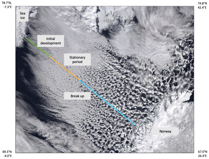
Figure 1Cloud development in a marine cold-air outbreak on 21 March 2021, moving from the ice edge to the Norwegian coastline in the bottom right. Source: NASA Worldview corrected reflectance (true colour) from the MODIS instrument on Terra.
Stratocumulus-to-cumulus transitions have been extensively studied for subtropical clouds using model simulation (e.g. Sandu and Stevens, 2011), satellite studies (e.g. Christensen et al., 2020) and in situ measurements (e.g. Sarkar et al., 2020). These studies have identified several causes as the driving force behind stratocumulus-to-cumulus transitions, such as an increasing sea surface temperature gradient and precipitation mediated by aerosol and ice-production processes. As air is advected over the relatively warm ocean surface, the strength of the turbulent surface fluxes deepens the boundary layer, eventually causing the cloud layer to be decoupled from the surface (Bretherton and Wyant, 1997; Sandu and Stevens, 2011). As the ocean surface is cut off as a source of moisture and aerosols, the stratocumulus decks eventually dissipate. However, the below-cloud layer continues to be warmed and moistened by the ocean surface, allowing cumuliform clouds in the lower boundary layer. Although primarily studied for subtropical clouds, McCoy et al. (2017) found that boundary layer instability and surface forcing were key drivers for developing open-cell cloud morphologies in MCAOs.
Precipitation can also facilitate the break-up of cloud fields; the evaporation of precipitation below the cloud cools and moistens the air of the sub-cloud layer (Stevens et al., 1998; Yamaguchi et al., 2017; Tornow et al., 2021). This cooling creates instability near the surface, which, in conjunction with the moistening effect, is favourable to the formation of cumuliform clouds (Stevens et al., 1998). All else being equal, earlier precipitation would cause a more rapid transition. Precipitation also reduces the lifetime of the stratiform cloud layer by the removal of water (Abel et al., 2017; Lloyd et al., 2018). Frozen precipitation, in particular, has been identified as key to breaking up the cloud field in MCAOs by accelerating the removal of cloud water through aerosol scavenging and mechanisms such as riming (Tornow et al., 2021) or secondary ice production (Abel et al., 2017; Karalis et al., 2022). Through modelling an MCAO north of the United Kingdom, Abel et al. (2017) found that precipitation, as opposed to the sea surface temperature gradient or entrainment drying of the cloud, was the key driver of cloud break-up.
Aerosols can strongly influence the onset of precipitation. A higher aerosol load generally leads to smaller liquid cloud droplets, which coalesce into precipitation-sized droplets more slowly, potentially delaying the transition (Albrecht, 1989; Yamaguchi et al., 2017; Goren et al., 2019). Once rainfall begins, often through the build-up of cloud water, the falling precipitation removes boundary layer aerosols, creating a negative aerosol gradient over the outbreak (Abel et al., 2017; Lloyd et al., 2018; Dadashazar et al., 2021). This aerosol scavenging creates a positive feedback loop, as fewer aerosols mean a reduced number of sites on which new droplets can form, causing droplets to grow sufficiently large to precipitate (Jing and Suzuki, 2018). Modelling studies suggest that higher initial cloud condensation nuclei (CCN) concentrations delay the formation of precipitation in MCAOs (Tornow et al., 2021). However, aerosols that can act as ice-nucleating particles (INPs) can potentially accelerate the transition through droplet riming and enhancing precipitation (Abel et al., 2017; Tornow et al., 2021).
Global and high-resolution models struggle to simulate evolution and properties of the low-level liquid and mixed-phase clouds often found in these outbreaks (Morrison et al., 2012; Field et al., 2014; Bodas-Salcedo et al., 2016; Abel et al., 2017; Field et al., 2017). The persistent negative biases in the short-wave reflectivity of Southern Ocean clouds in general circulation models have been attributed to the representation of supercooled liquid (Cesana et al., 2022). The radiative properties of supercooled liquid clouds – which are prevalent in the Arctic (Shupe, 2011; Cesana et al., 2012) – in a changing climate are of particular interest. The Arctic region is warming at a much faster rate than in lower latitudes (Serreze and Barry, 2011), leading to the ability to establish more industries and shipping routes as sea ice is lost. This will mean more aerosols are available to interact with clouds (Peters et al., 2011; Schmale et al., 2018; Maahn et al., 2021). As Arctic clouds strongly influence the surface energy budget (Curry and Ebert, 1992; Shupe and Intrieri, 2004), understanding potential changes in these clouds is essential for understanding future changes in the region.
The processes which affect the MCAO cloud evolution are fundamentally time-dependent, and knowledge of these process rates is essential for improving their representation in climate models (Pithan et al., 2018). Previous studies have used models (e.g Tornow et al., 2021), in situ or airborne measurements (Hartmann et al., 1997; Young et al., 2016; Abel et al., 2017; Lloyd et al., 2018; Ruiz-Donoso et al., 2020; Geerts et al., 2022), and satellites (Wu and Ovchinnikov, 2022) to investigate the factors influencing cloud property development during the course of an outbreak. However, these were typically based on a relatively small set of examples of MCAO events. Geostationary satellites have been used to study clouds along the stratocumulus-to-cumulus transition following a large collection of Lagrangian trajectories in the subtropics (e.g. Christensen et al., 2020), but they do not cover high latitudes well.
Polar-orbiting satellites can provide several consecutive images for a location at high latitudes, providing a unique opportunity to characterise the temporal development of clouds. To study this evolution, we generate composite trajectories of air parcels moving off the ice edge using reanalysis wind fields. These trajectories are co-located with reanalysis data and data from several satellite instruments to investigate the factors which influence liquid cloud properties during the course of the cold-air outbreak. In particular, we examine the controls on cloud properties that most strongly determine cloud albedo, namely cloud fraction and liquid water path (Loeb et al., 2007). The development of these cloud properties is then linked to changes in the top-of-atmosphere (TOA) albedo to estimate how these different environmental conditions affect the potential cloud radiative forcing.
2.1 Data
Cloud property data were obtained from the Moderate Resolution Imaging Spectroradiometer (MODIS) Level 2 Collection 6.1 data product (MYD06_L2, Platnick et al., 2017). The data were regridded to a 25 km by 25 km polar stereographic grid, and only those north of 60∘ latitude were included in this analysis. It is possible that clouds embedded in the outbreaks are obscured by higher-level overlying clouds; to limit this effect, L2 pixels with cloud top heights above 500 hPa were eliminated; Fletcher et al. (2016b) showed that clouds within outbreaks are typically lower than this. The “Cloud_Multi_Layer_Flag” was also used to filter the data to only include single-layer clouds. The period of study was between 2008 and 2014, inclusive. The area of interest is limited to the North Atlantic and Kara Sea region to avoid bias towards shorter trajectories (Sect. 2.2).
The Arctic environment provides many challenges to obtaining reliable satellite data, particularly those relating to cloud microphysical properties, such as the frequency of high solar-zenith angles (Kato and Marshak, 2009; Grosvenor and Wood, 2014) However, rigorous filtering of these data to remove particularly uncertain cases helps to limit the effects of these biases on the results. The cloud optical depth and cloud effective radius (re) were filtered and used to calculate the cloud liquid water path (LWP) and cloud droplet number concentration (Nd), following Murray-Watson and Gryspeerdt (2022). This filtering involved excluding pixels with high heterogeneity index (“Cloud_Mask_SPI” >30; Zhang and Platnick, 2011) and high solar-zenith angles (> 65∘) or high viewing angles (> 50∘) (Grosvenor and Wood, 2014). The LWP and Nd were calculated using Eqs. 1 (Wood and Hartmann, 2006) and 2 (Szczodrak et al., 2001; Quaas et al., 2006), respectively,
in which τc is the cloud optical thickness, and re is the cloud droplet effective radius. For the Nd calculations, additional filtering of re (> 4 µm) and τc (> 4) is used to minimise retrieval biases (Quaas et al., 2006; Sourdeval et al., 2016); this is not applied to the LWP as it would introduce a high bias in LWP (Gryspeerdt et al., 2019a). ρw is the density of water. A value of 0.8 is used for k, which is related to the droplet spectrum width (Painemal and Zuidema, 2011; Grosvenor and Wood, 2014). The extinction coefficient (Q) is assumed to be approximately equal to 2 (Bennartz, 2007). The temperature-dependent condensation rate is calculated following Gryspeerdt et al. (2016) and Grosvenor and Wood (2014), using the MODIS cloud top temperature, and a subadiabatic factor (fad) of 0.7 is assumed (Painemal and Zuidema, 2011). Equations (1) and (2) assume adiabatic conditions (Brenguier et al., 2000; Wood and Hartmann, 2006).
Although ice is often present in MCAO clouds (Fletcher et al., 2016b), the factors which influence ice-phase processes and phase transitions are challenging to study using satellite data. As such, this study focuses on the development of liquid-dominated MCAO clouds. Grid cells (25×25 km) in which the MODIS sensor detect a non-zero ice fraction are removed from the analysis. Although the MODIS optical property phase algorithm typically performs well in comparison to active sensors (Marchant et al., 2016), it is still unlikely that this filtering entirely removes ice clouds from the dataset. Additionally, only pixels with a cloud top temperature above 263 K are included; in situ measurements in the Arctic have shown that these clouds typically have very high liquid water fractions (de Boer et al., 2009). This filtering to remove ice reduces the dataset to 31 % of its original size.
DARDAR (raDAR/liDAR, Delanoë and Hogan, 2010; Ceccaldi et al., 2013), which is produced by combining lidar data from CALIOP (Winker et al., 2009) and radar data from CloudSat (Stephens et al., 2008), is used to analyse the efficacy of these filters to restrict the analysis to liquid-dominated clouds. Due to known issues with surface clutter affecting DARDAR retrievals, cases with cloud top heights below 720 m are not included. Figure 2 shows the DARDAR-retrieved cloud top phase fractions as a function of MODIS temperature for the set of MODIS pixels filtered to remove ice. The phase fraction is calculated as the number of DARDAR retrievals with a given phase flag divided by the number of DARDAR retrievals for each 25 km by 25 km grid box. For this analysis, DARDAR phase flags “Ice”, “Spherical_or_2D_ice” and “Highly_concentrated_ice” are together considered as “ice” and “Supercooled_and_ice” is considered “mixed phase”. Figure 2 indicates that with this filtering, the supercooled phase fraction starts at 73 % at 263 K and increases with temperature. Although DARDAR shows a non-negligible proportion of ice-containing phases, the real amount of ice present in these clouds is uncertain, as it would take a relatively small amount of ice to register a radar return and cause the retrieval to be classified as “mixed phase” (Bühl et al., 2013). Restricting this study to pixels where DARDAR only registers supercooled liquid clouds would also reduce the volume of data available for analysis to less than 5 % of the MODIS pixels co-located with the trajectories due to the DARDAR's nadir-only sampling. As such, the method used here for filtering out ice-containing pixels is deemed sufficient for this work. The potential effects of biases introduced by ice undetected by MODIS will be discussed more in Sect. 4.
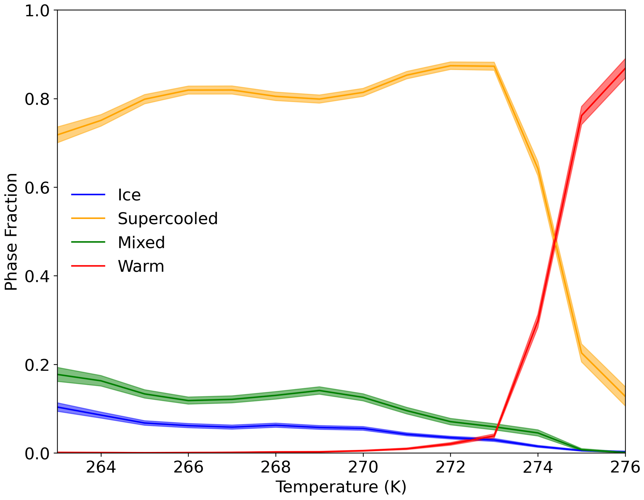
Figure 2DARDAR cloud top phase fraction binned against MODIS cloud top temperature for clouds following the trajectories generated in this study. DARDAR phase flags “Ice”, “Spherical_or_2D_ice” and “Highly_concentrated_ice” are combined to calculate the ice fraction. DARDAR flags “Supercooled”, “Liquid” and “Supercooled_and_ice” are considered to be “supercooled”, “warm” and “mixed”, respectively. Phase fraction is calculated by dividing the number of successful retrievals for a given phase flag by the total number of DARDAR retrievals for a 25 km by 25 km pixel. The shading represents the 95 % confidence interval.
Top-of-atmosphere (TOA) albedo data were obtained from hourly Clouds and the Earth's Radiant Energy System (CERES) SYN1deg L3 dataset NASA/LARC/SD/ASDC (2017). These data were regridded from the original 1×1∘ resolution to the same 25×25 km grid and projection as the MODIS data. Previous studies have shown that CERES TOA albedo measurements perform well over ocean (e.g. Sun et al., 2006; Kato et al., 2018) but are biased relative to in situ measurements if sea ice is present (e.g. Riihelä, et al., 2017; Huang et al., 2022).
Sea ice data were obtained from Nimbus-7 SMMR (Scanning Multichannel Microwave Radiometer) and Defense Meteorological Satellite Program Special Sensor Microwave/Imager and Special Sensor Microwave Imager/Sounder (DMSP SSM/I–SSMIS) Passive Microwave Data, Version 2, product (DiGirolamo et al., 2022). These data are produced in a 25 km resolution polar stereographic grid. A binary mask is created such that if there is any non-zero sea ice concentration, that pixel is considered sea ice, and ocean pixels are entirely ice-free (zero detected sea ice concentration). This may bias these results as some air parcels may be moving over relatively ice-free ocean before they are classified as having left the ice edge and being over ocean (see Sect. 2.2). However, MODIS struggles to retrieve cloud properties over sea ice (e.g. Chan and Comiso, 2013); the strict filtering of sea ice applied in this work helps to prevent potential cloud misclassification.
The meteorological reanalysis data were obtained from ERA5 (ECMWF Reanalysis v5) (Hersbach et al., 2020). The data were regridded to the same grid and projection as the MODIS data. The wind data at 1000 hPa were chosen to represent the boundary layer wind speed (following Gryspeerdt et al., 2021), and the specific humidity at 800 hPa was taken to represent the moisture conditions above the cloud top (based on mean cloud top pressure in MCAOs, Fig. 6g). The total aerosol optical depth at 550 nm (AOD) reanalysis data from the Copernicus Atmosphere Monitoring Services (CAMS; Inness et al., 2019) was used as an indicative measure of aerosol conditions in the region. These were regridded in a similar manner to the meteorological reanalysis data.
The marine cold-air outbreak index (M; Kolstad and Bracegirdle, 2008) is an important indicator of cloud formation and behaviour at high latitudes. It measures the stability of the boundary layer and is calculated as the difference between the potential temperature at 800 hPa and the sea surface temperature (Fletcher et al., 2016a), with positive values indicating higher instability. This metric is particularly suitable for the air moving off the ice edge as it highlights the difference in temperature of the relatively warm ocean with the cool overlying air masses. In the Northern Hemisphere, outbreak events are most common in the winter, followed by autumn and spring (Fletcher et al., 2016a). MCAOs are relatively rare in the summer. As some cloud properties, such as re, can only be retrieved during sunlight hours, this analysis is restricted from March to October each year. Figure 3 shows the mean MCAO index (M) within outbreaks (excluding times when M ≤ 0) and the relative frequency of occurrence of outbreaks (Fig. 3b) for March to October of 2008–2014. The data have been filtered to over-ocean values only following the extensive filtering described in this section.
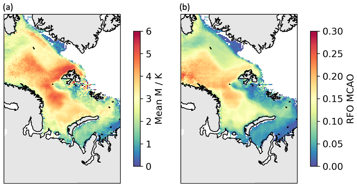
Figure 3MCAO index (M) calculated from ERA5 data for March–October of 2008–2014, filtered to only include MCAO events (M>0) (a) and the relative frequency of occurrence (RFO) for outbreaks (b). Grey represents the land, and white represents no data due to sea ice coverage.
2.2 Trajectory generation
ERA5 reanalysis wind fields, regridded to the same 25 km by 25 km grid as the MODIS data, were used to create the Lagrangian trajectories. Wind data at 1000 hPa were used for the advection, as this has previously been shown to follow low-level clouds successfully (following Gryspeerdt et al., 2019b). Examples of the trajectories generated by this method are shown in Fig. 4.
The advection procedure is adapted from Horner and Gryspeerdt (2022), which focuses on trajectories starting from points of new convection. Here, a similar method is used, but the initial points are identified as cases where the air has moved from being over sea ice to being over open ocean between time steps of 1 h. These pixels newly over the ocean are given a value of time since ice (TSI) of 1 h, and all other pixels which did not move from ice to ocean remain at zero (Fig. 4). Then, all pixels are advected forward again following the wind fields. For pixels previously identified as having moved off the ice edge in the first time step, 1 h is added to their TSI. Pixels newly over ocean are again identified and given TSI values of 1 h. This advection process repeats for every time step, with a value of one being added to all pixels on trajectories moving from the ice edge, a value of 1 h assigned to pixels newly over the ocean, and zero assigned to all other pixels. In addition to the TSI value, each pixel has a date and time associated with the wind fields used to produce it; this is used to co-locate these pixels with the satellite data. If pixels move over land or back over sea ice, the trajectory is no longer followed. When two trajectories of two or more pixels converge, the smaller TSI is taken as the value for that pixel. The mean TSI for the region of interest is shown in Fig. 5.
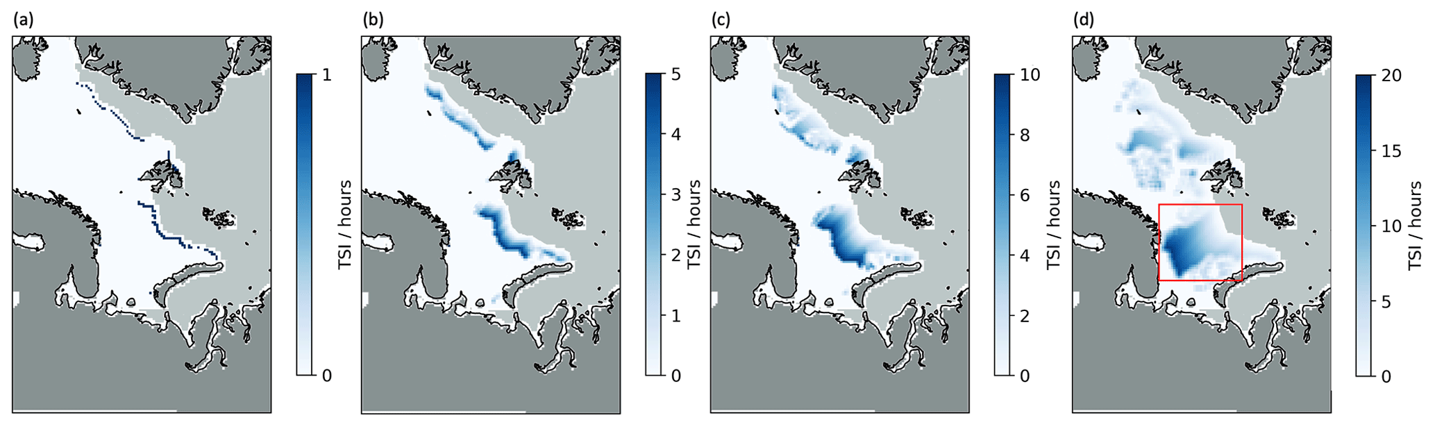
Figure 4Snapshot of the time-since-ice trajectory generation for (a) 1, (b) 5, (c) 10 and (d) 20 h since moving from the ice edge. Dark and light grey represent land and sea ice pixels, respectively. The scale varies between subplots. The red box in panel (d) indicates air moving off the ice edge that developed into a marine cold-air outbreak. The data are from 1 April 2014.
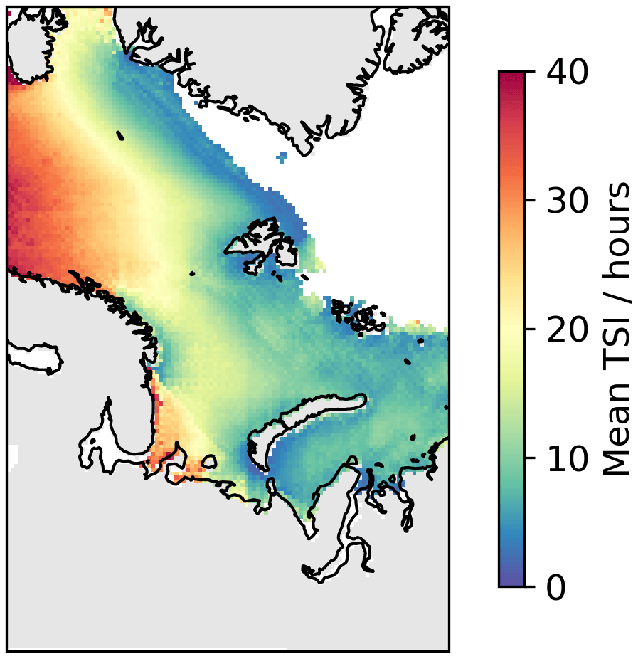
Figure 5Map of the average time since ice for trajectories generated between March and October of 2008–2014. Grey represents the land, and white represents no data due to sea ice coverage.
A set of reverse trajectories of air parcels travelling over the ocean towards the ice edge were generated by running the above process in reverse; cases which move from being over open ocean to being over ice between time steps in the forward direction are identified and then tracked backward in time. These are useful to compare to clouds moving away from the ice edge as the effects of any retrieval biases, particularly close to the ice edge, are revealed. Additionally, the clouds along these trajectories are effectively blind to the ice edge but travel through generally similar environmental conditions over the ocean to those moving off the ice edge. As a result, the changes in cloud properties resulting from moving off the ice edge can be highlighted. In these cases, time-towards-ice (TTI) pixel values indicate the number of hours before the clouds reach the ice edge along these trajectories (i.e. a TTI of 30 h means that, following this advection scheme, a pixel will reach the ice in 30 h).
3.1 Effects of moving off the ice edge
Figure 6 shows the development of cloud properties along three sets of trajectories: clouds approaching the ice edge (“Towards”), clouds not embedded in cold-air outbreaks (“non-MCAO”) moving away from the ice and those within outbreaks (“MCAO”). The MCAO and non-MCAO trajectories were partitioned based on the M value early on in the trajectory (M > 0 within the first 10 h of leaving the ice edge).
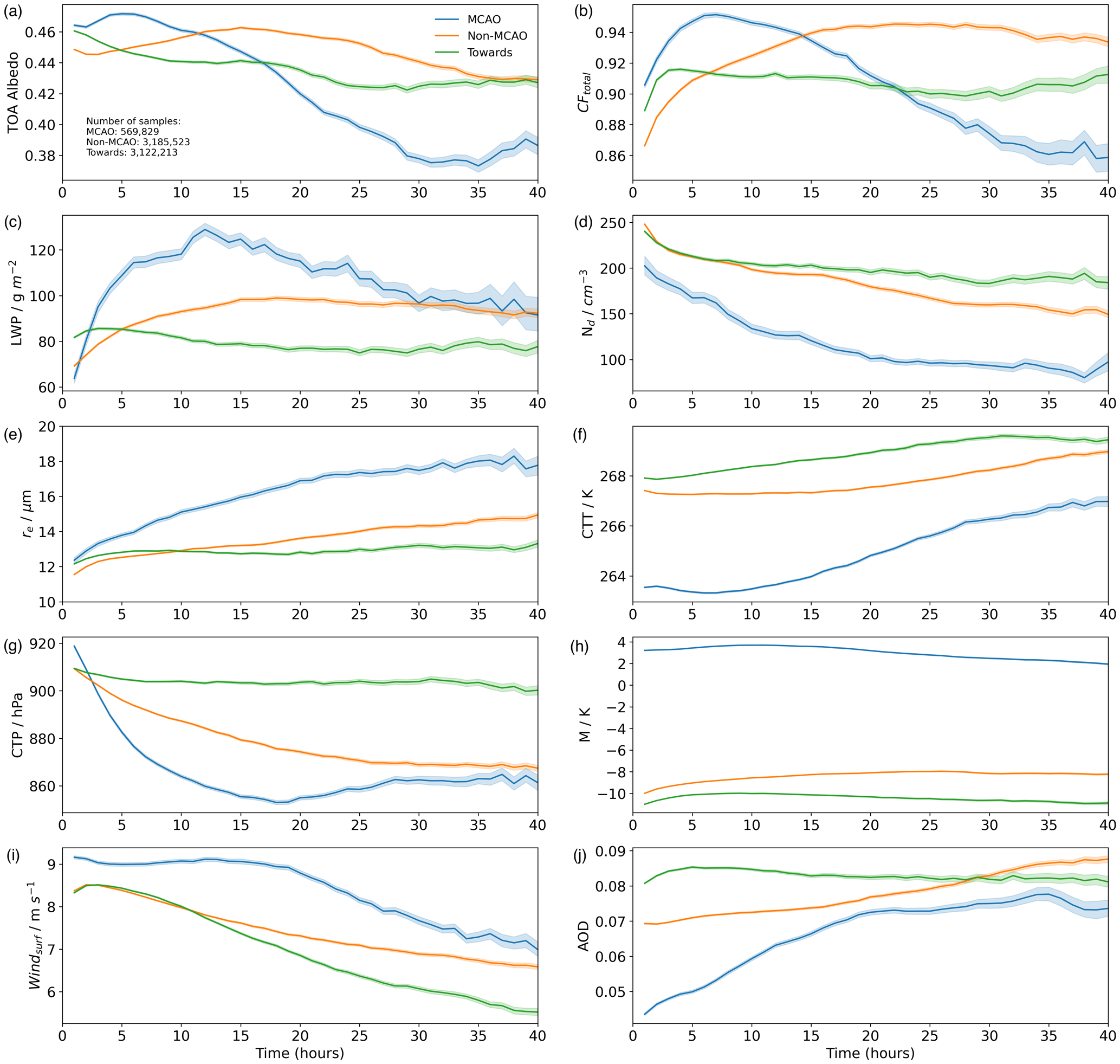
Figure 6Cloud properties and environmental conditions along the MCAO (blue), non-MCAO (orange) and Towards (green) trajectories. CERES data were used for panel (a), and data for panels (b)–(f) were obtained from the MODIS instrument. Reanalysis data were used for panels (g)–(j). For all of the trajectories, a time of 0 h represents the ice edge. For the MCAO and non-MCAO clouds, the time coordinate represents the time since ice, and their development moving from the ice edge proceeds from left to right in each subplot. For the Towards clouds, it is the time towards ice, or the number of hours until these air parcels reach the ice edge, and their development is instead read from right to left. The shading represents the 95 % confidence interval (found using bootstrapping). CTT and CTP are cloud top temperature and cloud top pressure, respectively.
3.1.1 Cloud fraction
Clouds moving towards the ice edge (the Towards trajectories) maintain a consistently high cloud fraction (between 90 % to 92 %; Fig. 6b) over the observation period, with a sharp decrease near the ice edge. This decrease may be because of a retrieval bias, but as it does not appear to affect any of the other measured properties, we expect this to have a negligible impact on the results. While high, these cloud fractions are typical for the region, particularly between spring and autumn in the Barents Sea, where most of the trajectories in this study were generated (Fig. 6a; Kay et al., 2016). Non-MCAO clouds slowly increase to a peak of 94 % at 22 h away from the ice and generally persist at this coverage for the remainder of the trajectory. After the crossover at 5 h, these clouds maintain a cloud fraction on average 3 % less than Towards clouds over the observation period. This difference between the non-MCAO and Towards clouds may in part be because while non-MCAO clouds are, by definition, not exposed to the extremely powerful fluxes generated in MCAO events, they still move through less stable environments (higher MCAO, Fig. 6h) with higher wind speeds (Fig. 6i), promoting cloud formation by transporting energy and moisture from the surface to the boundary layer.
MCAO clouds sharply increase in cloud fraction within a few hours of leaving the ice edge, reaching coverage of about 95 %. Between 7 and 40 h TSI time, the MCAO cloud fraction decreases at approximately −0.3 % h−1, with the cloud fraction falling below that of non-MCAO and Towards events at 14 and 22 h, respectively. This decrease in cloud fraction is due to the stratiform layers initially produced in MCAOs transitioning to the roll-like cumulus clouds, commonly observed in outbreaks (Fig. 1). The factors controlling the cloud fraction are discussed further in subsequent sections.
3.1.2 Liquid water path
The LWP of clouds moving towards the ice edge is generally steady, maintaining an average of around 80 g m−2 (Fig. 6c), which is in line with other liquid clouds in the region during spring to autumn (Shupe et al., 2006; Shupe, 2011). Non-MCAO clouds moving from the ice edge start with a lower LWP to these clouds but overtake them at around 5 h and remain on average 17 g m−2 higher for the rest of the trajectory, reaching a maximum of 100 g m−2 after 17 h. For both of these sets of clouds, there is little variability in LWP along the trajectory.
In contrast, MCAO clouds show a rapid initial increase in LWP within 5–6 h of leaving the ice, reaching a peak of around 127 g m−2 after 13 h. The LWP then begins to change at a rate of −1 g m−2 h−1 but remains higher than non-MCAO clouds for 40 h. This initial increase and then decline with LWP along the trajectory has been found in other studies examining the evolution of MCAO cloud properties (Abel et al., 2017; Lloyd et al., 2018; Tornow et al., 2021). This LWP evolution has been attributed to both the instability and precipitation mechanisms in previous works (Tornow et al., 2021, 2022). The unstable conditions promote the entrainment of subsaturated air into the cloud, thereby reducing the LWP through evaporation (Chen et al., 2014; Michibata et al., 2016). Figure 6e shows that precipitation is also key to LWP depletion, as the size of the droplets reaches 15 µm, considered to be precipitation-sized (Rosenfeld and Gutman, 1994), just before the LWP decline. As with cloud fraction, a combination of effects related to the instability and precipitation mechanisms is explored in the following sections.
3.1.3 Droplet number concentration
The Nd of clouds moving towards the ice edge increases over the trajectory, from about 200 to 250 cm−3 (Fig. 6d). For non-MCAO clouds, the Nd values are similar to the Towards clouds close to the ice edge but change at a rate of −2 cm−3 h−1 and fall below the Towards clouds after 7 h. For both of these trajectories, the values further from the ice edge are approximately the same or slightly higher than previous studies using MODIS have found (Zeng et al., 2014; McCoy et al., 2020), whereas the values close to the ice edge are higher. The larger Nd at the ice edge may be due to an increase in aerosol sources available in this biologically active zone (Leck and Persson, 1996) or the stronger winds (Fig. 6h) transporting aerosol to the cloud layer more efficiently. It is also possible that despite the extensive filtering of the satellite data, retrieval errors contribute to this increase near the ice edge. This extensive filtering has also likely biased the dataset used here relative to those used on other studies.
MCAO events start at lower Nd concentrations (200 cm−3) and decline at a rate of 4 cm−3 h−1 until about 25 h into the trajectory. From there, the Nd concentration is relatively steady at about 90–100 cm−3, which is on average 110 cm−3 lower than Towards clouds and 90 cm−3 lower than non-MCAO clouds. MCAO events may start at a lower Nd due to a potentially different origin of the air relative to non-MCAO events; the air may have travelled over ice for longer and is therefore cooler and cleaner than the non-MCAO air. Previous work has found that some air masses can travel over the sea ice for extended periods before reaching the ocean (Silber and Shupe, 2022); however, a full investigation is beyond the scope of this study. Previous work has found a similarly steep decline in Nd concentration following an MCAO (Abel et al., 2017; Sanchez et al., 2022). Two main drivers of this Nd gradient in MCAOs have been proposed: the dilution of aerosol concentration through entrainment of air from the free troposphere and precipitation scavenging of aerosol from the below-cloud layer, which are considered further below.
3.1.4 TOA albedo
For all sets of trajectories, the TOA albedo (Fig. 6a) generally follows the cloud fraction trend, as has been observed in previous studies (e.g. Loeb et al., 2007; Bender et al., 2011). The TOA albedo for Towards trajectories is generally steady between 0.42 and 0.44, until very close to the ice edge where it increases relatively sharply to 0.46. This increase may be due to the increases in LWP and Nd close to the ice edge (Fig. 6c and d), despite decreases in cloud cover, or it may be due to a bias introduced by undetected sea ice. Although initially high, the MCAO TAO albedo gradually decreases from about 0.47 to 0.37 after about 35 h, an albedo of about 0.06 below the non-MCAO and Towards clouds. Using CERES SYN1deg data, the average short-wave downwelling flux at 850 mbar (around the cloud top height; Fig. 6g) for the region of interest between March and October is calculated to be around 275 W m−2. Therefore, the albedo difference means about 16 W m−2 more radiation reaching the surface relative to non-MCAO trajectories post-transition. However, this reduced cooling effect is only present during the summer, when the short-wave cooling effect of clouds is relevant.
3.2 Effects of instability
The intensity of MCAO events is expected to change as the high latitudes warm (Kolstad and Bracegirdle, 2008); therefore, it is important to know how the MCAO strength affects the evolution of cloud properties. Fletcher et al. (2016b) found that for mid-latitude outbreaks, clouds embedded in stronger-MCAO events typically had higher cloud fractions and optical thickness, which enhanced their short-wave effect. However, whether this relationship between MCAO strength and cloud properties persists over the temporal development of the cloud is uncertain.
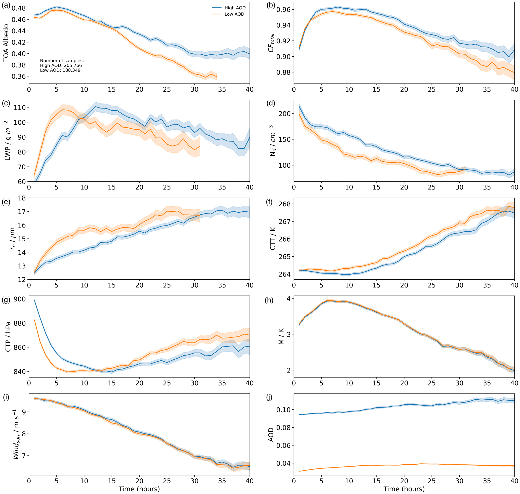
To characterise the influence of MCAO strength on cloud development, the MCAO trajectories are divided based on whether their initial MCAO index (within the first 10 h) fell into the upper or lower terciles of the M distribution (3.9 and 1.5 K, respectively, similar to Fletcher et al., 2016b). As aerosols are also known to affect cloud development (Sect. 4.3), the data are resampled such that the AOD distributions are equal for the strong- and weak-MCAO composites for each time step (following Gryspeerdt et al., 2014). The resampling method involves dividing the AOD distribution at each time step into bins for strong and weak trajectories and randomly sampling the bin of the trajectory with more points in it until it matches the trajectory with fewer points (as illustrated in Fig. 1 of Gryspeerdt et al., 2014). This is repeated for each time step. The results are shown in Fig. 7.

Figure 7As Fig. 6 but for strong (M > 3.9 K, blue) and weak (0 K K, orange) outbreak events moving away from the ice edge.
3.2.1 Cloud fraction
Initially, clouds embedded in strong-MCAO events have cloud fraction about 1 %–2 % higher than those in weak events (Fig. 7b). The strong-MCAO clouds maintain a high cloud fraction (94 %) for several hours but then decrease at a rate of 0.3 % h−1 after 7 h. The weak-MCAO cloud fraction begins to decline around the same time at a similar rate (0.2 % h−1). The gap in cloud coverage between the two trajectories closes at around 20 h, after which the strong-MCAO clouds are approximately 1 % lower for the remainder of the observation period. Although small, the difference in the rate of decline results in weaker-MCAO events having higher cloud coverage for longer; for instance, after 25 h, the strong-MCAO cloud fraction falls below 88 % – a level only reached 4 h later for weak-MCAO events.
This faster decrease in cloud fraction for stronger outbreaks is mirrored by the Nd development (Fig. 7d). Clouds in strong MCAOs start with much higher Nd than those in lower intensity outbreaks but fall steeply within the first 20 h (−7 cm−3 h−1), plateauing around 60–70 cm−3. In contrast, Nd in lower-MCAO events decreases more gradually over the first 24 h (−5 cm−3 h−1), steadying at about 10 cm−3 higher than the strong-MCAO case. These observations of cloud fraction development concur with previous work, showing an increase in aerosol or Nd associated with an increase in cloud fraction (Gryspeerdt et al., 2016; Goren et al., 2019; Chen et al., 2022). As in Sect. 3.1.3, the cause for the difference in Nd between strong and weak events may depend on factors such as how long the air has spent over ice; while this is beyond the scope of this present study, it should be accounted for in future work investigating the effect of MCAO strength on cloud development.
The steeper decline in Nd (and therefore cloud fraction) in the stronger outbreaks is potentially due to the stronger entrainment of drier, cleaner air (Fig. S1), leading to droplet evaporation and aerosol loss to the free troposphere (Tornow et al., 2022). The deeper boundary layer (implied by Fig. 7g) would also enhance decoupling from the surface and therefore prevent the surface from acting as a source of moisture and aerosols, enhancing the decline in Nd and hence cloud fraction. Another contributing factor to the more rapid Nd decline could be driven by collision–coalescence prior to precipitation; stronger outbreaks have higher LWP (Fig. 7c), which contributes strongly to the rain rate and accelerates collision–coalescence (Pawlowska and Brenguier, 2003) and therefore may reduce Nd. For both strong and weak events, precipitation is likely to be a factor in the very strong Nd decline early in the development. Although Fig. 7 shows that the average droplet is below the commonly used 15 µm threshold for precipitation, Fig. S2 indicates that there are still a significant proportion of precipitation-sized droplets present in these clouds. It is also possible that undetected ice crystals may enhance precipitation and Nd loss through droplet riming (Tornow et al., 2021).
3.2.2 Liquid water path
Instability has little relationship to LWP for the first few hours of cloud development (Fig. 7c). However, after 5 h, the LWP in strong-MCAO events continues to increase, reaching a maximum of about 135 g m−2 at 13 h. Following this peak, the strong-MCAO LWP decreases at a rate of approximately 3 g m−2 h−1. Conversely, the weak-MCAO LWP remains around 100 g m−2 until 15 h from ice, after which it decreases at a slower rate than the strong-MCAO cases (−1 g m−2 h−1). Until around 33 h, the weak-MCAO cases maintain a LWP of about 20–30 g m−2 lower than the strong-MCAO composite. Although entrainment drying would be enhanced in less stable conditions, the strong-MCAO clouds have a higher LWP to start with due to the heat and moisture fluxes associated with these events (Fletcher et al., 2016a), which also allow the clouds to grow deeper (implied by lower CTP in Fig. 6g).
For both sets of trajectories, the timing of the LWP decline is nearly coincident with the point at which the mean droplet reaches the precipitation collision–coalescence threshold (15 µm, Fig. 7e), indicating the importance of precipitation to cloud break-up. Despite having an impact on the magnitude of the LWP increase, the MCAO strength does not appear to strongly modify the timing of the transition; the point at which LWP begins to decrease is only 2 to 3 h earlier in the strong outbreaks. This may be due to the competing effects of LWP and Nd on precipitation (Goren et al., 2022); in strong-MCAO events, LWP is high (which promotes precipitation), but higher Nd also suppresses precipitation. Conversely, in weaker events, lower LWP hinders precipitation, while low Nd enhances precipitation formation. Therefore, the effects of LWP and Nd act as a buffer against each other in strong- and weak-MCAO events, leading to both trajectories reaching the 15 µm point at approximately the same time. It should be noted that the smaller droplet effective radius in clouds embedded in stronger outbreaks (Fig. 7e) is counter-intuitive, given these clouds are deeper than those in weaker outbreaks (Fig. 7g). This may be due to some unknown aerosol sources which are not well represented in the reanalysis data, meaning the attempts to constrain the effects of aerosols are not fully effective.
3.2.3 TOA albedo
Despite the differences in the evolution of the macro- and micro-physical properties, there is a negligible difference (0.01–0.02) between the scene albedo over the course of the strong- and weak-MCAO trajectories. This may be due to the competing effects on the albedo; although the cloud fraction of the strong events does fall slightly below the weaker events over time, the enhanced LWP compensates for this decline, leading to roughly similar reflectivities. This suggests that should the MCAO strength change with the changing climate (e.g. Kolstad and Bracegirdle, 2008), the impact on the short-wave energy budget due to changes in cloud properties may be minimal.
3.3 Effects of aerosol on cloud development
Aerosols can affect the transition from stratocumulus decks to broken cloud fields, influencing the timing of precipitation (e.g Christensen et al., 2020). In MCAOs, higher aerosol loads can delay the formation of the cumuliform regime (Tornow et al., 2021, 2022). However, once precipitation occurs, the aerosol scavenging accelerates the cloud field's break-up through enhanced water loss from the stratocumulus layer (Abel et al., 2017; Lloyd et al., 2018). The timescales over which aerosols modulate MCAO cloud development have not previously been studied with observational data.
To characterise these timescales, the MCAO trajectories are divided into above and below median (0.06) aerosol conditions based on the AOD early in their trajectory (within the first 10 h). As previously discussed, AOD from reanalysis is imperfect, especially in the Arctic, with aerosol sources potentially missing from the data product. Furthermore, the vertical profile of the aerosol load is important to clouds in MCAOs; Tornow et al. (2022) showed that entrainment of free-tropospheric air may reduce the aerosol burden in MCAOs. As AOD is a column-integrated value, it does not describe the aerosol concentration throughout the cloud. Additionally, the AOD does not differentiate between INPs and CCN, which is important considering the differing roles they play in cloud lifetime. However, INP concentrations are typically less abundant than CCN by several orders of magnitude (e.g. Bigg and Leck, 2001). Here, the AOD is used qualitatively to indicate whether the trajectories are moving through more or less aerosol-laden conditions.
The influence of boundary layer instability on cloud development is constrained using the resampling method discussed in Sect. 4.2 on M for each time step. Additionally, as the wind speed is also known to affect cloud properties (such as cloud fraction; Engström and Ekman, 2010), it is also resampled to be the same for the high- and low-AOD trajectories. The M and wind speed distributions are resampled sequentially. In this work, M is resampled before the wind speed, but as the two are highly correlated, the order of which variable is resampled first has little effect on the results (not shown).
3.3.1 Cloud fraction
Figure 8b shows that there is initially a small difference in cloud fraction between the high- and low-AOD cases. However, after about 3 h, the effects of aerosol become apparent and the trajectories diverge. The high-AOD case reaches 96 % coverage and maintains this level until about 10 h from ice, after which it decreases at a rate of about 0.2 % h−1. The low-AOD cases remain about 1 %–2 % lower, with the difference growing over time. As before, the cloud fraction evolution is mirrored by the Nd development in both high- and low-AOD conditions. Initially, the Nd for both trajectories is similar, but the decrease in Nd in cleaner conditions is more rapid than in cases with more aerosol (−6 cm−3 h−1 versus −4 cm−3 h−1).
As M and wind speed are accounted for by the resampling, both the dilution of aerosol to the free troposphere and ability of the surface to act as a source are similar in both high- and low-AOD cases. Therefore, the difference between the two sets of outbreaks is likely due to enhanced precipitation earlier in the low-aerosol trajectories. Figure 8e shows that the cloud droplets grow in size more quickly in cleaner conditions and reach precipitation size about 6–7 h. Higher aerosol loads mean cloud droplets stay smaller for longer, keeping the Nd higher and maintaining a higher cloud coverage for a longer time.
3.3.2 Liquid water path
In contrast to the effects of outbreak strength, which strongly modulated the peak LWP but not the timing, changes in aerosol conditions influence the point of LWP decline but only moderately affect peak LWP magnitude (Fig. 8c). Clouds in low-AOD trajectories have a much earlier peak in LWP (about 108 g m−2 at 5–7 h) than clouds in high-AOD trajectories (112 g m−2 at 12 h). The LWP decreases in both sets of trajectories are closely linked to precipitation dynamics; the point at which re reaches 15 µm is within 1–2 h of the start of the LWP decline in both cases. As with the cloud fraction cases, more aerosols lead to precipitation suppression, which allows the LWP to build up more gradually. However, due to the build-up of cloud water, precipitation eventually still occurs, triggering the transition. The near doubling of the time to the LWP peak highlights the potentially significant effect that aerosols, through influencing precipitation dynamics, can have on the cloud development.
3.3.3 TOA albedo
As would be expected from the cloud fraction and LWP development, the TOA albedo declines more slowly in high-AOD trajectories. Although the difference in albedo is initially small, the composites diverge over time, eventually growing to 0.04 after about 30 h. This approximately corresponds to an additional 11 W m−2 (using the regional average short-wave downwelling radiation at 850 mbar) of cooling in summer due to the prolonged high cloud cover and delayed LWP peak. This cooling is not insignificant; Huang et al. (2017) found that anomalies in the short-wave cooling of a similar magnitude caused by changes in cloud properties during late spring and early summer influenced the extent of sea ice melt.
3.4 Stability-dependent aerosol effect
Section 3.3 considered the effects of an aerosol perturbation while constraining the instability; however, previous work has shown that the cloud response to aerosols can change depending on the stability environment (Murray-Watson and Gryspeerdt, 2022). Therefore, the response of cloud properties to aerosols may depend on the strength of the MCAO. Figure 9 shows the effects of dividing the MCAO trajectories into four regimes: strong/weak MCAO and high/low aerosol, based on the upper and lower M terciles and median AOD, as in previous sections. To highlight the overall differences in responses between clouds in strong and weak events, M is constrained to be identical along high-/low-aerosol trajectories for each case.
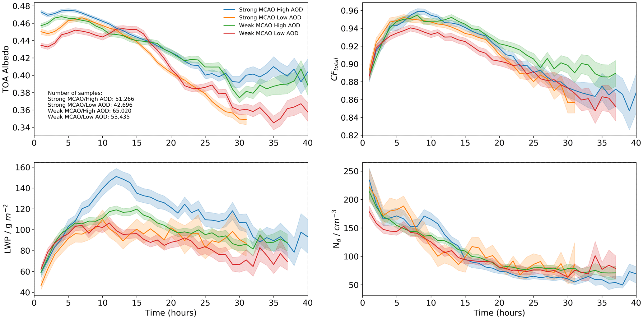
Figure 9As Fig. 6 but for trajectories in strong-/weak-MCAO and high-/low-aerosol conditions.
In general, the effects of aerosols on clouds in strong and weak events is similar to that seen in Sect. 3.3; clouds in higher-aerosol conditions typically have higher cloud fractions (Fig. 9b) and delayed peak in LWP (Fig. 9c), leading to a higher albedo (Fig. 9a). In strong-MCAO events, the difference in albedo between the high- and low-aerosol conditions appears to be driven by the large difference in LWP, with relatively little difference in cloud fraction between the two cases. However, both the cloud fraction and the LWP contribute to the higher albedo in the weak-MCAO/high-AOD cases. Previous work has shown that in relatively clean conditions, as the aerosol load increases, less stable conditions typically have a higher LWP than stable conditions (Murray-Watson and Gryspeerdt, 2022), potentially explaining the difference in LWP response between strong and weak events in Fig. 9c. However, it is unclear why the aerosol load does not strongly affect the cloud coverage in strong-MCAO events; the large surface fluxes may be the dominant term in promoting cloud formation, leaving little sensitivity to aerosol.
This work presents a novel way of investigating the temporal development of cloud properties during cold-air outbreaks by creating composite trajectories and co-locating these with satellite and reanalysis data. Through comparison with clouds in non-MCAO events, the extent to which the extreme turbulent fluxes affect the cloud development and formation are revealed. Many of the results here confirm what has been observed in model results or field campaigns; deep, high-coverage clouds form quickly as the air moves from the ice edge. Eventually, through precipitation, these clouds transition into thinner, low-coverage cloud fields. The cloud microphysical properties also evolve throughout the outbreak; Nd declines and LWP initially builds up before decreasing. The unique aspect of this study is the insight into the timescales for these processes occurring and the ability to use reanalysis data to probe the mechanisms controlling these cloud properties.
When considering the effects of MCAO strength, these composite trajectories reveal the importance of considering how far the clouds are along the outbreak. Fletcher et al. (2016b) found that clouds in stronger outbreaks had higher cloud fraction and optical thickness and therefore a greater short-wave cooling effect. However, weak- and strong-outbreak cases were selected based on the value of M for a given grid box. Figure 7g shows that M decreases over the course of a trajectory, particularly for strong events, so that selection by grid box is actually choosing clouds at different points in their development. Although initially lower, weak outbreaks actually maintain a higher coverage for longer. However, due to the enhanced LWP in stronger outbreaks, this does not translate to a strong change in TOA albedo or short-wave cooling effect of the cloud.
Due to changes in the Arctic climate, the strength and frequency of MCAOs are expected to change in the future. Several modelling studies have projected an overall decrease in the M, except in areas of sea ice retreat, where M will increase due to the availability of the ocean surface (Kolstad and Bracegirdle, 2008; Landgren et al., 2019). Figure 7 suggests that a shift in the MCAO strength would not strongly shift the short-wave cooling effect of the clouds, due to the competing factors controlling the TOA albedo. However, should the MCAO weaken so much that they constitute “non-MCAO” events moving off the ice edge, there would be a shift to higher-albedo, more-cooling clouds over their trajectories (Fig. 6a). The data presented here only consider MCAO events during sunlit months, where the short-wave cooling effects of low-level clouds over the ocean surface are expected to be dominant over the long-wave warming. However, MCAOs are most common during winter (Fletcher et al., 2016a), when a lack of sunlight precludes the analysis of some cloud properties. Although Fletcher et al. (2016b) found that MCAO strength, rather than season, was the strongest determinant of cloud properties, the generalisability of the results presented here is uncertain. However, if these results hold, it would be the long-wave warming effect of the clouds which is most relevant. As the clouds in this study typically have an emissivity near unity (for LWP > 30 g m−2; Shupe and Intrieri, 2004), the cloud long-wave effect is predominantly controlled by cloud cover. If the MCAO-CF relationship holds in a future Arctic, this suggests that a weakening of the MCAO would generate longer-lasting, more-warming clouds.
As more aerosol sources such as industry or shipping move further into the Arctic, from Fig. 8, it appears that should these aerosols interact with clouds in MCAOs, they would lead to longer-lived stratocumulus fields, and these higher-coverage, thicker clouds would have either a stronger warming or cooling effect, depending on the season. These results highlight that knowledge of the aerosol environment close to the ice edge is essential to model the development of these clouds correctly. Despite recent efforts, such as the measurement of aerosols capable of ice nucleation during the Multidisciplinary drifting Observatory for the Study of Arctic Climate (MOSAiC) expedition (Creamean et al., 2022; Shupe et al., 2022), the aerosol sources and sinks close to the ice edge are not well characterised, thus leaving models poorly constrained. Given the effects that aerosols have on the timing of the cloud transition, this uncertainty around aerosol sources may make it difficult to determine the radiative impact of these clouds.
This work solely focuses on liquid-dominant clouds embedded in MCAOs, limiting ourselves to only a third of all available data. However, clouds embedded in MCAOs are often mixed phase, with lower ice concentrations in the stratocumulus decks and increasing in the cumulus fields (Abel et al., 2017; Lloyd et al., 2018). These ice crystals can be important in cloud development, and although efforts have been made to exclude the influence of these ice crystals, it is possible that undetected ice may introduce some bias into the results. Ice crystals may rime the liquid droplets, enhancing precipitation and contributing to the steep Nd gradient in Fig. 7d. Additionally, if an ice crystal is misclassified as liquid water, it may produce a higher measurement for the liquid droplet effective radius due to the different scattering and absorption properties of ice crystals (Platnick et al., 2003). This would lead to an underestimation in Nd and overestimation of LWP. Figure 7e shows that stronger events – typically associated with more ice (Fletcher et al., 2016b) – have a lower re than lower-MCAO clouds, suggesting that this is not the dominant effect. However, it is possible that ice undetected by MODIS has a non-negligible influence on these results.
Clouds in marine cold-air outbreaks undergo a characteristic evolution, transforming from high-coverage, stratiform clouds to a broken, low-coverage cumuliform cloud field. Despite previous flight and measurement campaigns, models struggle to capture this development due to the complex set of factors controlling cloud properties. This work uses a set of composite trajectories to develop a time-resolved picture of how cloud properties change as air moves away from the ice edge and the effect of different environmental conditions on the cloud evolution.
MCAO cloud properties are distinct from clouds following other non-MCAO trajectories (Fig. 6b–e). The cloud albedo is largely controlled by cloud fraction, so as the clouds transition from high- to low-coverage cloud fields during an outbreak, their short-wave cooling effect weakens. The cloud fraction in turn is strongly correlated with the Nd, a relationship seen in previous studies and which holds across the range of factors considered here. Similarly, along each set of composite trajectories, the timing of the LWP peak is nearly coincident with the point at which the mean re reaches 15 µm, indicating the importance of precipitation to cloud transition.
The initial MCAO strength has a lasting impact on the cloud property development, which is particularly visible in the LWP (Fig. 7c). Previous work investigating the impact of MCAO strength on clouds has considered a grid-box-by-grid-box approach rather than how clouds develop as the outbreak progresses. These results show that for some cloud properties (such as the cloud fraction, Fig. 7b), clouds in strong-MCAO events typically start with a higher cloud fraction, as had been seen in previous studies, but this does not hold at later stages of development. However, despite differences in cloud property development, the opposing influences of the cloud fraction and LWP development mean that the TOA albedo for clouds in each set of composite trajectories is very similar (Fig. 7a). Furthermore, the timing of the transition is not strongly changed by the MCAO strength.
In contrast, a higher initial aerosol load delayed the transition by 5–7 h and slowed the decline in cloud fraction, enhancing the TOA short-wave cooling by approximately 11 W m−2 relative to low-aerosol conditions (Fig. 8). This suggests that in a future, more polluted Arctic, these new aerosols sources may increase the cloud cooling effect through delaying the stratocumulus-to-cumulus transition. This potentially strong impact on cloud development and radiative properties highlights the need to constrain sources of Arctic aerosols, particularly close to the ice edge.
The MODIS data were obtained from NASA Goddard Space Flight Center (https://modis.gsfc.nasa.gov/data/, Platnick et al., 2017). The ERA5 data were obtained from the Climate Data Store (https://cds.climate.copernicus.eu/cdsapp#!/dataset/reanalysis-era5-complete, Hersbach et al., 2020), and the CAMS reanalysis was obtained from the Atmospheric Data Store (https://ads.atmosphere.copernicus.eu/cdsapp#!/dataset/cams-global-reanalysis-eac4, Inness et al., 2019). The sea ice data were obtained from the National Snow and Ice Data Center (https://nsidc.org/data/nsidc-0051/versions/2, DiGirolamo et al., 2022). The CERES data were downloaded from the NASA Langley Research Center (https://ceres.larc.nasa.485 gov/data/#syn1deg-level-3, NASA/LARC/SD/ASDC, 2017).
The supplement related to this article is available online at: https://doi.org/10.5194/acp-23-9365-2023-supplement.
RJMW and EG contributed to the study design, and all authors were involved with the interpretation of results. RJMW performed the analysis and prepared the manuscript, with comments from EG and TG.
The contact author has declared that none of the authors has any competing interests.
Publisher’s note: Copernicus Publications remains neutral with regard to jurisdictional claims in published maps and institutional affiliations.
Rebecca J. Murray-Watson and Edward Gryspeerdt were supported by funding from the Royal Society (University Research Fellowship, URF/R1/191602). Tom Goren acknowledges funding by the German Research Foundation (Deutsche Forschungsgemeinschaft, DFG, project “CDNC4ACI”, GZ QU 311/27-1). We thank George Horner for his insight on generating the composite trajectories.
This research has been supported by the Royal Society (grant no. URF/R1/191602) and the Deutsche Forschungsgemeinschaft (grant no. GZ QU 311/27-1).
This paper was edited by Thijs Heus and reviewed by Israel Silber and one anonymous referee.
Abel, S. J., Boutle, I. A., Waite, K., Fox, S., Brown, P. R. A., Cotton, R., Lloyd, G., Choularton, T. W., and Bower, K. N.: The Role of Precipitation in Controlling the Transition from Stratocumulus to Cumulus Clouds in a Northern Hemisphere Cold-Air Outbreak, J. Atmos. Sci., 74, 2293–2314, https://doi.org/10.1175/JAS-D-16-0362.1, 2017. a, b, c, d, e, f, g, h, i, j, k
Albrecht, B. A.: Aerosols, Cloud Microphysics, and Fractional Cloudiness, Science, 245, 1227–1230, https://doi.org/10.1126/science.245.4923.1227, 1989. a
Bender, F. A.-M., Charlson, R. J., Ekman, A. M. L., and Leahy, L. V.: Quantification of Monthly Mean Regional-Scale Albedo of Marine Stratiform Clouds in Satellite Observations and GCMs, J. Appl. Meteorol. Climatol., 50, 2139–2148, https://doi.org/10.1175/JAMC-D-11-049.1, 2011. a
Bennartz, R.: Global assessment of marine boundary layer cloud droplet number concentration from satellite, J. Geophys. Res.-Atmos., 112, D02201, https://doi.org/10.1029/2006JD007547, 2007. a
Bigg, E. K. and Leck, C.: Cloud-active particles over the central Arctic Ocean, J. Geophys. Res.-Atmos., 106, 32155–32166, https://doi.org/10.1029/1999JD901152, 2001. a
Bodas-Salcedo, A., Andrews, T., Karmalkar, A. V., and Ringer, M. A.: Cloud liquid water path and radiative feedbacks over the Southern Ocean, Geophys. Res. Lett., 43, 10938–10946, https://doi.org/10.1002/2016GL070770, 2016. a
Boucher, O., Randall, D., Artaxo, P., Bretherton, C., Feingold, G., Forster, P., Kerminen, V.-M., Kondo, Y., Liao, H., Lohmann, U., Rasch, P., Satheesh, S. K., Sherwood, S., Stevens, B., and Zhang, X. Y.: Clouds and aerosols, in: Climate Change 2013: The Physical Science Basis, Contribution of Working Group I to the Fifth Assessment Report of the Intergovernmental Panel on Climate Change, edited by: Stocker, T. F., Qin, D., Plattner, G.-K., Tignor, M., Allen, S. K., Doschung, J., Nauels, A., Xia, Y., Bex, V., and Midgley, P. M., 571–657, Cambridge University Press, Cambridge, UK, https://doi.org/10.1017/CBO9781107415324.016, 2013. a
Brenguier, J.-L., Pawlowska, H., Schüller, L., Preusker, R., Fischer, J., and Fouquart, Y.: Radiative Properties of Boundary Layer Clouds: Droplet Effective Radius versus Number Concentration, J. Atmos. Sci., 57, 803–821, https://doi.org/10.1175/1520-0469(2000)057<0803:RPOBLC>2.0.CO;2, 2000. a
Bretherton, C. S. and Wyant, M. C.: Moisture Transport, Lower-Tropospheric Stability, and Decoupling of Cloud-Topped Boundary Layers, J. Atmos. Sci., 54, 148–167, https://doi.org/10.1175/1520-0469(1997)054<0148:MTLTSA>2.0.CO;2, 1997. a
Brümmer, B.: Boundary-layer modification in wintertime cold-air outbreaks from the Arctic sea ice, Bound.-Lay. Meteorol., 80, 109–125, https://doi.org/10.1007/BF00119014, 1996. a
Brümmer, B.: Roll and Cell Convection in Wintertime Arctic Cold-Air Outbreaks, J. Atmos. Sci., 56, 2613–2636, https://doi.org/10.1175/1520-0469(1999)056<2613:RACCIW>2.0.CO;2, 1999. a
Bühl, J., Ansmann, A., Seifert, P., Baars, H., and Engelmann, R.: Toward a quantitative characterization of heterogeneous ice formation with lidar/radar: Comparison of CALIPSO/CloudSat with ground-based observations, Geophys. Res. Lett., 40, 4404–4408, https://doi.org/10.1002/grl.50792, 2013. a
Ceccaldi, M., Delanoë, J., Hogan, R. J., Pounder, N. L., Protat, A., and Pelon, J.: From CloudSat-CALIPSO to EarthCare: Evolution of the DARDAR cloud classification and its comparison to airborne radar-lidar observations, J. Geophys. Res.-Atmos., 118, 7962–7981, https://doi.org/10.1002/jgrd.50579, 2013. a
Cesana, G., Kay, J. E., Chepfer, H., English, J. M., and de Boer, G.: Ubiquitous low-level liquid-containing Arctic clouds: New observations and climate model constraints from CALIPSO-GOCCP, Geophys. Res. Lett., 39, L20804, https://doi.org/10.1029/2012GL053385, 2012. a
Cesana, G. V., Khadir, T., Chepfer, H., and Chiriaco, M.: Southern Ocean Solar Reflection Biases in CMIP6 Models Linked to Cloud Phase and Vertical Structure Representations, Geophys. Res. Lett., 49, e2022GL099777, https://doi.org/10.1029/2022GL099777, 2022. a
Chan, M. A. and Comiso, J. C.: Arctic Cloud Characteristics as Derived from MODIS, CALIPSO, and CloudSat, J. Clim., 26, 3285–3306, https://doi.org/10.1175/JCLI-D-12-00204.1, 2013. a
Chen, Y., Haywood, J., Wang, Y., Malavelle, F., Jordan, G., Partridge, D., Fieldsend, J., De Leeuw, J., Schmidt, A., Cho, N., Oreopoulos, L., Platnick, S., Grosvenor, D., Field, P., and Lohmann, U.: Machine learning reveals climate forcing from aerosols is dominated by increased cloud cover, Nat. Geosci., 15, 609–614, https://doi.org/10.1038/s41561-022-00991-6, 2022. a
Chen, Y.-C., Christensen, M., Stephens, G., and Seinfeld, J.: Satellite-based estimate of global aerosol–cloud radiative forcing by marine warm clouds, Nat. Geosci., 7, 643–646, https://doi.org/10.1038/ngeo2214, 2014. a
Choi, Y.-S., Kim, B.-M., Hur, S.-K., Kim, S.-J., Kim, J.-H., and Ho, C.-H.: Connecting early summer cloud-controlled sunlight and late summer sea ice in the Arctic, J. Geophys. Res.-Atmos., 119, 11087–11099, https://doi.org/10.1002/2014JD022013, 2014. a
Christensen, M. W., Jones, W. K., and Stier, P.: Aerosols enhance cloud lifetime and brightness along the stratus-to-cumulus transition, P. Natl. Acad. Sci. USA, 117, 17591–17598, https://doi.org/10.1073/pnas.1921231117, 2020. a, b, c
Creamean, J. M., Barry, K., Hill, T. C. J., Hume, C., DeMott, P. J., Shupe, M. D., Dahlke, S., Willmes, S., Schmale, J., Beck, I., Hoppe, C. J. M., Fong, A., Chamberlain, E., Bowman, J., Scharien, R., and Persson, O.: Annual cycle observations of aerosols capable of ice formation in central Arctic clouds, Nat. Commun., 13, 3537, https://doi.org/10.1038/s41467-022-31182-x, 2022. a
Curry, J. A. and Ebert, E. E.: Annual Cycle of Radiation Fluxes over the Arctic Ocean: Sensitivity to Cloud Optical Properties, J. Clim., 5, 1267–1280, https://doi.org/10.1175/1520-0442(1992)005<1267:ACORFO>2.0.CO;2, 1992. a
Dadashazar, H., Painemal, D., Alipanah, M., Brunke, M., Chellappan, S., Corral, A. F., Crosbie, E., Kirschler, S., Liu, H., Moore, R. H., Robinson, C., Scarino, A. J., Shook, M., Sinclair, K., Thornhill, K. L., Voigt, C., Wang, H., Winstead, E., Zeng, X., Ziemba, L., Zuidema, P., and Sorooshian, A.: Cloud drop number concentrations over the western North Atlantic Ocean: seasonal cycle, aerosol interrelationships, and other influential factors, Atmos. Chem. Phys., 21, 10499–10526, https://doi.org/10.5194/acp-21-10499-2021, 2021. a
de Boer, G., Eloranta, E. W., and Shupe, M. D.: Arctic Mixed-Phase Stratiform Cloud Properties from Multiple Years of Surface-Based Measurements at Two High-Latitude Locations, J. Atmos. Sci., 66, 2874–2887, https://doi.org/10.1175/2009JAS3029.1, 2009. a
Delanoë, J. and Hogan, R. J.: Combined CloudSat-CALIPSO-MODIS retrievals of the properties of ice clouds, J. Geophys. Res.-Atmos., 115, D00H29, https://doi.org/10.1029/2009JD012346, 2010. a
DiGirolamo, N., Parkinson, C. L., D. J. Cavalieri, P. G., and Zwally., H. J.: Sea Ice Concentrations from Nimbus-7 SMMR and DMSP SSM/I-SSMIS Passive Microwave Data, Version 2, https://doi.org/10.5067/MPYG15WAA4WX, 2022. a, b
Engström, A. and Ekman, A. M. L.: Impact of meteorological factors on the correlation between aerosol optical depth and cloud fraction, Geophys. Res. Lett., 37, L18814, https://doi.org/10.1029/2010GL044361, 2010. a
Field, P. R., Cotton, R. J., McBeath, K., Lock, A. P., Webster, S., and Allan, R. P.: Improving a convection-permitting model simulation of a cold air outbreak, Q. J. Roy. Meteor. Soc., 140, 124–138, https://doi.org/10.1002/qj.2116, 2014. a
Field, P. R., Broz̆ková, R., Chen, M., Dudhia, J., Lac, C., Hara, T., Honnert, R., Olson, J., Siebesma, P., de Roode, S., Tomassini, L., Hill, A., and McTaggart-Cowan, R.: Exploring the convective grey zone with regional simulations of a cold air outbreak, Q. J. Roy. Meteor. Soc., 143, 2537–2555, https://doi.org/10.1002/qj.3105, 2017. a
Fletcher, J., Mason, S., and Jakob, C.: The Climatology, Meteorology, and Boundary Layer Structure of Marine Cold Air Outbreaks in Both Hemispheres, J. Clim., 29, 1999–2014, https://doi.org/10.1175/JCLI-D-15-0268.1, 2016a. a, b, c, d, e, f
Fletcher, J. K., Mason, S., and Jakob, C.: A Climatology of Clouds in Marine Cold Air Outbreaks in Both Hemispheres, J. Clim., 29, 6677–6692, https://doi.org/10.1175/JCLI-D-15-0783.1, 2016b. a, b, c, d, e, f, g
Geerts, B., Giangrande, S. E., McFarquhar, G. M., Xue, L., Abel, S. J., Comstock, J. M., Crewell, S., DeMott, P. J., Ebell, K., Field, P., Hill, T. C. J., Hunzinger, A., Jensen, M. P., Johnson, K. L., Juliano, T. W., Kollias, P., Kosovic, B., Lackner, C., Luke, E., Lüpkes, C., Matthews, A. A., Neggers, R., Ovchinnikov, M., Powers, H., Shupe, M. D., Spengler, T., Swanson, B. E., Tjernström, M., Theisen, A. K., Wales, N. A., Wang, Y., Wendisch, M., and Wu, P.: The COMBLE campaign: a study of marine boundary-layer clouds in Arctic cold-air outbreaks, Bull. Am. Meteorol. Soc., 1, E1371–E1389, https://doi.org/10.1175/BAMS-D-21-0044.1, 2022. a
Goren, T., Kazil, J., Hoffmann, F., Yamaguchi, T., and Feingold, G.: Anthropogenic Air Pollution Delays Marine Stratocumulus Breakup to Open Cells, Geophys. Res. Lett., 46, 14135–14144, https://doi.org/10.1029/2019GL085412, 2019. a, b
Goren, T., Feingold, G., Gryspeerdt, E., Kazil, J., Kretzschmar, J., Jia, H., and Quaas, J.: Projecting Stratocumulus Transitions on the Albedo – Cloud Fraction Relationship Reveals Linearity of Albedo to Droplet Concentrations, Geophys. Res. Lett., 49, e2022GL101169, https://doi.org/10.1029/2022GL101169, 2022. a
Grosvenor, D. P. and Wood, R.: The effect of solar zenith angle on MODIS cloud optical and microphysical retrievals within marine liquid water clouds, Atmos. Chem. Phys., 14, 7291–7321, https://doi.org/10.5194/acp-14-7291-2014, 2014. a, b, c, d
Gryspeerdt, E., Stier, P., and Partridge, D. G.: Satellite observations of cloud regime development: the role of aerosol processes, Atmos. Chem. Phys., 14, 1141–1158, https://doi.org/10.5194/acp-14-1141-2014, 2014. a, b
Gryspeerdt, E., Quaas, J., and Bellouin, N.: Constraining the aerosol influence on cloud fraction, J. Geophys. Res.-Atmos., 121, 3566–3583, https://doi.org/10.1002/2015JD023744, 2016. a, b
Gryspeerdt, E., Goren, T., Sourdeval, O., Quaas, J., Mülmenstädt, J., Dipu, S., Unglaub, C., Gettelman, A., and Christensen, M.: Constraining the aerosol influence on cloud liquid water path, Atmos. Chem. Phys., 19, 5331–5347, https://doi.org/10.5194/acp-19-5331-2019, 2019a. a
Gryspeerdt, E., Smith, T. W. P., O'Keeffe, E., Christensen, M. W., and Goldsworth, F. W.: The Impact of Ship Emission Controls Recorded by Cloud Properties, Geophys. Res. Lett., 46, 12547–12555, https://doi.org/10.1029/2019GL084700, 2019b. a
Gryspeerdt, E., Goren, T., and Smith, T. W. P.: Observing the timescales of aerosol–cloud interactions in snapshot satellite images, Atmos. Chem. Phys., 21, 6093–6109, https://doi.org/10.5194/acp-21-6093-2021, 2021. a
Hartmann, J., Kottmeier, C., and Raasch, S.: Roll Vortices and Boundary-Layer Development during a Cold Air Outbreak, Bound.-Lay. Meteorol., 84, 45–65, https://doi.org/10.1023/A:1000392931768, 1997. a
Hersbach, H., Bell, B., Berrisford, P., Hirahara, S., Horányi, A., Muñoz-Sabater, J., Nicolas, J., Peubey, C., Radu, R., Schepers, D., Simmons, A., Soci, C., Abdalla, S., Abellan, X., Balsamo, G., Bechtold, P., Biavati, G., Bidlot, J., Bonavita, M., De Chiara, G., Dahlgren, P., Dee, D., Diamantakis, M., Dragani, R., Flemming, J., Forbes, R., Fuentes, M., Geer, A., Haimberger, L., Healy, S., Hogan, R. J., Hólm, E., Janisková, M., Keeley, S., Laloyaux, P., Lopez, P., Lupu, C., Radnoti, G., de Rosnay, P., Rozum, I., Vamborg, F., Villaume, S., and Thépaut, J.-N.: The ERA5 global reanalysis, Q. J. Roy. Meteor. Soc., 146, 1999–2049, https://doi.org/10.1002/qj.3803, 2020. a, b
Horner, G. A. and Gryspeerdt, E.: The evolution of deep convective systems and their associated cirrus outflows, Atmos. Chem. Phys. Discuss. [preprint], https://doi.org/10.5194/acp-2022-755, in review, 2022. a
Huang, Y., Dong, X., Xi, B., Dolinar, E. K., and Stanfield, R. E.: The footprints of 16 year trends of Arctic springtime cloud and radiation properties on September sea ice retreat, J. Geophys. Res.-Atmos., 122, 2179–2193, https://doi.org/10.1002/2016JD026020, 2017. a
Huang, Y., Taylor, P. C., Rose, F. G., Rutan, D. A., Shupe, M. D., Webster, M. A., and Smith, M. M.: Toward a more realistic representation of surface albedo in NASA CERES-derived surface radiative fluxes: A comparison with the MOSAiC field campaign: Comparison of CERES and MOSAiC surface radiation fluxes, Elementa, 10, 1, https://doi.org/10.1525/elementa.2022.00013, 00013, 2022. a
Inness, A., Ades, M., Agustí-Panareda, A., Barré, J., Benedictow, A., Blechschmidt, A.-M., Dominguez, J. J., Engelen, R., Eskes, H., Flemming, J., Huijnen, V., Jones, L., Kipling, Z., Massart, S., Parrington, M., Peuch, V.-H., Razinger, M., Remy, S., Schulz, M., and Suttie, M.: The CAMS reanalysis of atmospheric composition, Atmos. Chem. Phys., 19, 3515–3556, https://doi.org/10.5194/acp-19-3515-2019, 2019. a, b
Jing, X. and Suzuki, K.: The Impact of Process-Based Warm Rain Constraints on the Aerosol Indirect Effect, Geophys. Res. Lett., 45, 10729–10737, https://doi.org/10.1029/2018GL079956, 2018. a
Karalis, M., Sotiropoulou, G., Abel, S. J., Bossioli, E., Georgakaki, P., Methymaki, G., Nenes, A., and Tombrou, M.: Effects of secondary ice processes on a stratocumulus to cumulus transition during a cold-air outbreak, Atmos. Res., 277, 106302, https://doi.org/10.1016/j.atmosres.2022.106302, 2022. a
Kato, S. and Marshak, A.: Solar zenith and viewing geometry-dependent errors in satellite retrieved cloud optical thickness: Marine stratocumulus case, J. Geophys. Res.-Atmos., 114, 4501–4527, https://doi.org/10.1029/2008JD010579, 2009. a
Kato, S., Rose, F. G., Rutan, D. A., Thorsen, T. J., Loeb, N. G., Doelling, D. R., Huang, X., Smith, W. L., Su, W., and Ham, S.-H.: Surface Irradiances of Edition 4.0 Clouds and the Earth’s Radiant Energy System (CERES) Energy Balanced and Filled (EBAF) Data Product, J. Clim., 31, 4501–4527, https://doi.org/10.1175/JCLI-D-17-0523.1, 2018. a
Kay, J., L'Ecuyer, T., Chepfer, H., Loeb, N., Morrison, A., and Cesana, G.: Recent Advances in Arctic Cloud and Climate Research, Curr. Clim. Change Rep., 2, 159–169, https://doi.org/10.1007/s40641-016-0051-9, 2016. a
Khanal, S. and Wang, Z.: Uncertainties in MODIS-Based Cloud Liquid Water Path Retrievals at High Latitudes Due to Mixed-Phase Clouds and Cloud Top Height Inhomogeneity, J. Geophys. Res.-Atmos., 123, 11154–11172, https://doi.org/10.1029/2018JD028558, 2018. a
Klein, S. A. and Hartmann, D. L.: The Seasonal Cycle of Low Stratiform Clouds, J. Clim., 6, 1587–1606, https://doi.org/10.1175/1520-0442(1993)006<1587:TSCOLS>2.0.CO;2, 1993. a
Kolstad, E. W.: Higher ocean wind speeds during marine cold air outbreaks, Q. J. Roy. Meteor. Soc., 143, 2084–2092, https://doi.org/10.1002/qj.3068, 2017. a
Kolstad, E. W. and Bracegirdle, T. J.: Marine cold-air outbreaks in the future: an assessment of IPCC AR4 model results for the Northern Hemisphere, Clim. Dynam., 30, 871–885, https://doi.org/10.1007/s00382-007-0331-0, 2008. a, b, c, d
Landgren, O. A., Seierstad, I. A., and Iversen, T.: Projected future changes in Marine Cold-Air Outbreaks associated with Polar Lows in the Northern North-Atlantic Ocean, Clim. Dynam., 53, 2573–2585, https://doi.org/10.1007/s00382-019-04642-2, 2019. a
Leck, C. and Persson, C.: The central Arctic Ocean as a source of dimethyl sulfide Seasonal variability in relation to biological activity, Tellus B, 48, 156–177, https://doi.org/10.3402/tellusb.v48i2.15834, 1996. a
Lloyd, G., Choularton, T. W., Bower, K. N., Gallagher, M. W., Crosier, J., O'Shea, S., Abel, S. J., Fox, S., Cotton, R., and Boutle, I. A.: In situ measurements of cloud microphysical and aerosol properties during the break-up of stratocumulus cloud layers in cold air outbreaks over the North Atlantic, Atmos. Chem. Phys., 18, 17191–17206, https://doi.org/10.5194/acp-18-17191-2018, 2018. a, b, c, d, e, f
Loeb, N. G., Wielicki, B. A., Rose, F. G., and Doelling, D. R.: Variability in global top-of-atmosphere shortwave radiation between 2000 and 2005, Geophys. Res. Lett., 34, L03704, https://doi.org/10.1029/2006GL028196, 2007. a, b
Maahn, M., Goren, T., Shupe, M. D., and de Boer, G.: Liquid Containing Clouds at the North Slope of Alaska Demonstrate Sensitivity to Local Industrial Aerosol Emissions, Geophys. Res. Lett., 48, e2021GL094307, https://doi.org/10.1029/2021GL094307, 2021. a
Marchant, B., Platnick, S., Meyer, K., Arnold, G. T., and Riedi, J.: MODIS Collection 6 shortwave-derived cloud phase classification algorithm and comparisons with CALIOP, Atmos. Meas. Tech., 9, 1587–1599, https://doi.org/10.5194/amt-9-1587-2016, 2016. a
McCoy, I. L., Wood, R., and Fletcher, J. K.: Identifying Meteorological Controls on Open and Closed Mesoscale Cellular Convection Associated with Marine Cold Air Outbreaks, J. Geophys. Res.-Atmos., 122, 11678–11702, https://doi.org/10.1002/2017JD027031, 2017. a, b
McCoy, I. L., McCoy, D. T., Wood, R., Regayre, L., Watson-Parris, D., Grosvenor, D. P., Mulcahy, J. P., Hu, Y., Bender, F. A.-M., Field, P. R., Carslaw, K. S., and Gordon, H.: The hemispheric contrast in cloud microphysical properties constrains aerosol forcing, P. Natl. Acad. Sci. USA, 117, 18998–19006, https://doi.org/10.1073/pnas.1922502117, 2020. a
Michibata, T., Suzuki, K., Sato, Y., and Takemura, T.: The source of discrepancies in aerosol–cloud–precipitation interactions between GCM and A-Train retrievals, Atmos. Chem. Phys., 16, 15413–15424, https://doi.org/10.5194/acp-16-15413-2016, 2016. a
Morrison, H., de Boer, G., Feingold, G., Harrington, J., Shupe, M. D., and Sulia, K.: Resilience of persistent Arctic mixed-phase clouds, Nat. Geosci., 5, 11–17, https://doi.org/10.1038/ngeo1332, 2012. a
Murray-Watson, R. J. and Gryspeerdt, E.: Stability-dependent increases in liquid water with droplet number in the Arctic, Atmos. Chem. Phys., 22, 5743–5756, https://doi.org/10.5194/acp-22-5743-2022, 2022. a, b, c
NASA/LARC/SD/ASDC: CERES and GEO-Enhanced TOA, Within-Atmosphere and Surface Fluxes, Clouds and Aerosols 1-Hourly Terra-Aqua Edition4A, https://doi.org/10.5067/TERRA+AQUA/CERES/SYN1DEG-1HOUR_L3.004A, 2017. a, b
Painemal, D. and Zuidema, P.: Assessment of MODIS cloud effective radius and optical thickness retrievals over the Southeast Pacific with VOCALS-REx in situ measurements, J. Geophys. Res.-Atmos., 116, D24206, https://doi.org/10.1029/2011JD016155, 2011. a, b
Papritz, L. and Spengler, T.: A Lagrangian Climatology of Wintertime Cold Air Outbreaks in the Irminger and Nordic Seas and Their Role in Shaping Air–Sea Heat Fluxes, J. Clim., 30, 2717–2737, https://doi.org/10.1175/JCLI-D-16-0605.1, 2017. a
Pawlowska, H. and Brenguier, J.-L.: An observational study of drizzle formation in stratocumulus clouds for general circulation model (GCM) parameterizations, J. Geophys. Res.-Atmos., 108, 8630, https://doi.org/10.1029/2002JD002679, 2003. a
Peters, G. P., Nilssen, T. B., Lindholt, L., Eide, M. S., Glomsrød, S., Eide, L. I., and Fuglestvedt, J. S.: Future emissions from shipping and petroleum activities in the Arctic, Atmos. Chem. Phys., 11, 5305–5320, https://doi.org/10.5194/acp-11-5305-2011, 2011. a
Pithan, F., Svensson, G., Caballero, R., Chechin, D., Cronin, T. W., Ekman, A. M. L., Neggers, R., Shupe, M. D., Solomon, A., Tjernström, M., and Wendisch, M.: Role of air-mass transformations in exchange between the Arctic and mid-latitudes, Nat. Geosci., 11, 805–812, https://doi.org/10.1038/s41561-018-0234-1, 2018. a, b
Platnick, S., King, M. D., Ackerman, S. A., Menzel, W. P., Baum, B. A., Riedi, J. C., and Frey, R. A.: The MODIS cloud products: algorithms and examples from Terra, IEEE Trans. Geosci. Remote Sens., 41, 459–473, https://doi.org/10.1109/TGRS.2002.808301, 2003. a
Platnick, S., Meyer, K. G., King, M. D., Wind, G., Amarasinghe, N., Marchant, B., Arnold, G. T., Zhang, Z., Hubanks, P. A., Holz, R. E., Yang, P., Ridgway, W. L., and Riedi, J.: The MODIS Cloud Optical and Microphysical Products: Collection 6 Updates and Examples From Terra and Aqua, IEEE Trans. Geosci. Remote Sens., 55, 502–525, https://doi.org/10.1109/TGRS.2016.2610522, 2017. a, b
Quaas, J., Boucher, O., and Lohmann, U.: Constraining the total aerosol indirect effect in the LMDZ and ECHAM4 GCMs using MODIS satellite data, Atmos. Chem. Phys., 6, 947–955, https://doi.org/10.5194/acp-6-947-2006, 2006. a, b
Riihelä, A., Key, J. R.., Meirink, J. F., Kuipers Munneke, P., Palo, T., and Karlsson, K.-G.: An intercomparison and validation of satellite-based surface radiative energy flux estimates over the Arctic, J. Geophys. Res.-Atmos., 122, 4829–4848, https://doi.org/10.1002/2016JD026443, 2017. a
Rosenfeld, D. and Gutman, G.: Retrieving microphysical properties near the tops of potential rain clouds by multispectral analysis of AVHRR data, Atmos. Res., 34, 259–283, https://doi.org/10.1016/0169-8095(94)90096-5, 1994. a
Ruiz-Donoso, E., Ehrlich, A., Schäfer, M., Jäkel, E., Schemann, V., Crewell, S., Mech, M., Kulla, B. S., Kliesch, L.-L., Neuber, R., and Wendisch, M.: Small-scale structure of thermodynamic phase in Arctic mixed-phase clouds observed by airborne remote sensing during a cold air outbreak and a warm air advection event, Atmos. Chem. Phys., 20, 5487–5511, https://doi.org/10.5194/acp-20-5487-2020, 2020. a
Sanchez, K. J., Zhang, B., Liu, H., Brown, M. D., Crosbie, E. C., Gallo, F., Hair, J. W., Hostetler, C. A., Jordan, C. E., Robinson, C. E., Scarino, A. J., Shingler, T. J., Shook, M. A., Thornhill, K. L., Wiggins, E. B., Winstead, E. L., Ziemba, L. D., Saliba, G., Lewis, S. L., Russell, L. M., Quinn, P. K., Bates, T. S., Porter, J., Bell, T. G., Gaube, P., Saltzman, E. S., Behrenfeld, M. J., and Moore, R. H.: North Atlantic Ocean SST-gradient-driven variations in aerosol and cloud evolution along Lagrangian cold-air outbreak trajectories, Atmos. Chem. Phys., 22, 2795–2815, https://doi.org/10.5194/acp-22-2795-2022, 2022. a
Sandu, I. and Stevens, B.: On the Factors Modulating the Stratocumulus to Cumulus Transitions, J. Atmos. Sci., 68, 1865–1881, https://doi.org/10.1175/2011JAS3614.1, 2011. a, b
Sarkar, M., Zuidema, P., Albrecht, B., Ghate, V., Jensen, J., Mohrmann, J., and Wood, R.: Observations Pertaining to Precipitation within the Northeast Pacific Stratocumulus-to-Cumulus Transition, Mon. Weather Rev., 148, 1251–1273, https://doi.org/10.1175/MWR-D-19-0235.1, 2020. a
Schmale, J., Arnold, S. R., Law, K. S., Thorp, T., Anenberg, S., Simpson, W. R., Mao, J., and Pratt, K. A.: Local Arctic Air Pollution: A Neglected but Serious Problem, Earth's Future, 6, 1385–1412, https://doi.org/10.1029/2018EF000952, 2018. a
Schmale, J., Zieger, P., and Ekman, A.: Aerosols in current and future Arctic climate, Nat. Clim. Change, 11, 95–105, https://doi.org/10.1038/s41558-020-00969-5, 2021. a
Serreze, M. C. and Barry, R. G.: Processes and impacts of Arctic amplification: A research synthesis, Glob. Planet. Change, 77, 85–96, https://doi.org/10.1016/j.gloplacha.2011.03.004, 2011. a
Shupe, M. D.: Clouds at Arctic Atmospheric Observatories. Part II: Thermodynamic Phase Characteristics, J. Appl. Meteorol. Climatol., 50, 645–661, https://doi.org/10.1175/2010JAMC2468.1, 2011. a, b
Shupe, M. D. and Intrieri, J. M.: Cloud Radiative Forcing of the Arctic Surface: The Influence of Cloud Properties, Surface Albedo, and Solar Zenith Angle, J. Clim., 17, 616–628, https://doi.org/10.1175/1520-0442(2004)017<0616:CRFOTA>2.0.CO;2, 2004. a, b, c
Shupe, M. D., Matrosov, S. Y., and Uttal, T.: Arctic Mixed-Phase Cloud Properties Derived from Surface-Based Sensors at SHEBA, J. Atmos. Sci., 63, 697–711, https://doi.org/10.1175/JAS3659.1, 2006. a
Shupe, M. D., Rex, M., Blomquist, B., Persson, P. O. G., Schmale, J., Uttal, T., Althausen, D., Angot, H., Archer, S., Bariteau, L., Beck, I., Bilberry, J., Bucci, S., Buck, C., Boyer, M., Brasseur, Z., Brooks, I. M., Calmer, R., Cassano, J., Castro, V., Chu, D., Costa, D., Cox, C. J., Creamean, J., Crewell, S., Dahlke, S., Damm, E., de Boer, G., Deckelmann, H., Dethloff, K., Dütsch, M., Ebell, K., Ehrlich, A., Ellis, J., Engelmann, R., Fong, A. A., Frey, M. M., Gallagher, M. R., Ganzeveld, L., Gradinger, R., Graeser, J., Greenamyer, V., Griesche, H., Griffiths, S., Hamilton, J., Heinemann, G., Helmig, D., Herber, A., Heuzé, C., Hofer, J., Houchens, T., Howard, D., Inoue, J., Jacobi, H.-W., Jaiser, R., Jokinen, T., Jourdan, O., Jozef, G., King, W., Kirchgaessner, A., Klingebiel, M., Krassovski, M., Krumpen, T., Lampert, A., Landing, W., Laurila, T., Lawrence, D., Lonardi, M., Loose, B., Lüpkes, C., Maahn, M., Macke, A., Maslowski, W., Marsay, C., Maturilli, M., Mech, M., Morris, S., Moser, M., Nicolaus, M., Ortega, P., Osborn, J., Pätzold, F., Perovich, D. K., Petäjä, T., Pilz, C., Pirazzini, R., Posman, K., Powers, H., Pratt, K. A., Preußer, A., Quéléver, L., Radenz, M., Rabe, B., Rinke, A., Sachs, T., Schulz, A., Siebert, H., Silva, T., Solomon, A., Sommerfeld, A., Spreen, G., Stephens, M., Stohl, A., Svensson, G., Uin, J., Viegas, J., Voigt, C., von der Gathen, P., Wehner, B., Welker, J. M., Wendisch, M., Werner, M., Xie, Z., and Yue, F.: Overview of the MOSAiC expedition: Atmosphere, Elementa, 10, 00060, https://doi.org/10.1525/elementa.2021.00060, 2022. a
Silber, I. and Shupe, M. D.: Insights on sources and formation mechanisms of liquid-bearing clouds over MOSAiC examined from a Lagrangian framework, Elementa, 10, 000071, https://doi.org/10.1525/elementa.2021.000071, 2022. a
Sourdeval, O., C.-Labonnote, L., Baran, A. J., Mülmenstädt, J., and Brogniez, G.: A methodology for simultaneous retrieval of ice and liquid water cloud properties, Part 2: Near-global retrievals and evaluation against A-Train products, Q. J. Roy. Meteor. Soc., 142, 3063–3081, https://doi.org/10.1002/qj.2889, 2016. a
Stephens, G. L., Vane, D. G., Tanelli, S., Im, E., Durden, S., Rokey, M., Reinke, D., Partain, P., Mace, G. G., Austin, R., L'Ecuyer, T., Haynes, J., Lebsock, M., Suzuki, K., Waliser, D., Wu, D., Kay, J., Gettelman, A., Wang, Z., and Marchand, R.: CloudSat mission: Performance and early science after the first year of operation, J. Geophys. Res.-Atmos., 113, D00A18, https://doi.org/10.1029/2008JD009982, 2008. a
Stevens, B., Cotton, W. R., Feingold, G., and Moeng, C.-H.: Large-Eddy Simulations of Strongly Precipitating, Shallow, Stratocumulus-Topped Boundary Layers, J. Atmos. Sci., 55, 3616–3638, https://doi.org/10.1175/1520-0469(1998)055<3616:LESOSP>2.0.CO;2, 1998. a, b
Sun, W., Loeb, N. G., Davies, R., Loukachine, K., and Miller, W. F.: Comparison of MISR and CERES top-of-atmosphere albedo, Geophys. Res. Lett., 33, L23810, https://doi.org/10.1029/2006GL027958, 2006. a
Szczodrak, M., Austin, P. H., and Krummel, P. B.: Variability of Optical Depth and Effective Radius in Marine Stratocumulus Clouds, J. Atmos. Sci., 58, 2912–2926, https://doi.org/10.1175/1520-0469(2001)058<2912:VOODAE>2.0.CO;2, 2001. a
Tornow, F., Ackerman, A. S., and Fridlind, A. M.: Preconditioning of overcast-to-broken cloud transitions by riming in marine cold air outbreaks, Atmos. Chem. Phys., 21, 12049–12067, https://doi.org/10.5194/acp-21-12049-2021, 2021. a, b, c, d, e, f, g, h, i
Tornow, F., Ackerman, A. S., Fridlind, A. M., Cairns, B., Crosbie, E. C., Kirschler, S., Moore, R. H., Painemal, D., Robinson, C. E., Seethala, C., Shook, M. A., Voigt, C., Winstead, E. L., Ziemba, L. D., Zuidema, P., and Sorooshian, A.: Dilution of Boundary Layer Cloud Condensation Nucleus Concentrations by Free Tropospheric Entrainment During Marine Cold Air Outbreaks, Geophys. Res. Lett., 49, e2022GL098444, https://doi.org/10.1029/2022GL098444, 2022. a, b, c, d
Winker, D. M., Vaughan, M. A., Omar, A., Hu, Y., Powell, K. A., Liu, Z., Hunt, W. H., and Young, S. A.: Overview of the CALIPSO Mission and CALIOP Data Processing Algorithms, J. Atmos. Ocean. Technol., 26, 2310–2323, https://doi.org/10.1175/2009JTECHA1281.1, 2009. a
Wood, R. and Hartmann, D. L.: Spatial Variability of Liquid Water Path in Marine Low Cloud: The Importance of Mesoscale Cellular Convection, J. Clim., 19, 1748–1764, https://doi.org/10.1175/JCLI3702.1, 2006. a, b
Wu, P. and Ovchinnikov, M.: Cloud Morphology Evolution in Arctic Cold-Air Outbreak: Two Cases During COMBLE Period, J. Geophys. Res.-Atmos., 127, e2021JD035966, https://doi.org/10.1029/2021JD035966, 2022. a
Yamaguchi, T., Feingold, G., and Kazil, J.: Stratocumulus to Cumulus Transition by Drizzle, J. Adv. Model. Earth Syst., 9, 2333–2349, https://doi.org/10.1002/2017MS001104, 2017. a, b
Young, G., Jones, H. M., Choularton, T. W., Crosier, J., Bower, K. N., Gallagher, M. W., Davies, R. S., Renfrew, I. A., Elvidge, A. D., Darbyshire, E., Marenco, F., Brown, P. R. A., Ricketts, H. M. A., Connolly, P. J., Lloyd, G., Williams, P. I., Allan, J. D., Taylor, J. W., Liu, D., and Flynn, M. J.: Observed microphysical changes in Arctic mixed-phase clouds when transitioning from sea ice to open ocean, Atmos. Chem. Phys., 16, 13945–13967, https://doi.org/10.5194/acp-16-13945-2016, 2016. a
Zeng, S., Riedi, J., Trepte, C. R., Winker, D. M., and Hu, Y.-X.: Study of global cloud droplet number concentration with A-Train satellites, Atmos. Chem. Phys., 14, 7125–7134, https://doi.org/10.5194/acp-14-7125-2014, 2014. a
Zhang, Z. and Platnick, S.: An assessment of differences between cloud effective particle radius retrievals for marine water clouds from three MODIS spectral bands, J. Geophys. Res.-Atmos., 116, D20215, https://doi.org/10.1029/2011JD016216, 2011. a