the Creative Commons Attribution 4.0 License.
the Creative Commons Attribution 4.0 License.
 | 21 Aug 2023
Effects of storage conditions on the molecular-level composition of organic aerosol particles
Julian Resch
Kate Wolfer
Alexandre Barth
Markus Kalberer
A significant fraction of atmospheric aerosol particles, which affect both the Earth's climate and human health, can be attributed to organic compounds and especially to secondary organic aerosol (SOA). To better understand the sources and processes generating organic aerosol particles, detailed chemical characterization is necessary, and particles are often collected onto filters and subsequently analyzed by liquid chromatography–mass spectrometry (LC–MS). A downside of such offline analysis techniques is the uncertainty regarding artifactual changes in composition occurring during sample collection, storage, extraction and analysis. The goal of this work was to characterize how storage conditions and storage time can affect the chemical composition of SOA generated from β-pinene and naphthalene, as well as from urban atmospheric aerosol samples. SOA samples were produced in the laboratory using an aerosol flow tube and were collected onto PTFE filters, whereas ambient samples were collected onto quartz filters with a high-volume air sampler. To characterize temporal changes in SOA composition, all samples were extracted and analyzed immediately after collection but were also stored as aqueous extracts or as filters for 24 h and up to 4 weeks at three different temperatures of +20, −20 or −80 ∘C in order to assess whether a lower storage temperature would be favorable. Analysis was conducted using ultra-high-performance liquid chromatography–high-resolution mass spectrometry (UHPLC–HRMS). Both principal component analysis (PCA) and time series of selected compounds were analyzed to identify the compositional changes over time. We show that the chemical composition of organic aerosols remained stable during low-temperature storage conditions, while storage at room temperature led to significant changes over time, even at short storage times of only 1 d. This indicates that it is necessary to freeze samples immediately after collection, and this requirement is especially important when automated ambient sampling devices are used where filters might be stored in the device for several days before being transferred to a laboratory.
- Article
(2491 KB) - Full-text XML
-
Supplement
(1500 KB) - BibTeX
- EndNote


Organic aerosol (OA), and especially secondary organic aerosol (SOA), constitutes a large fraction of atmospheric fine particulate matter (PM2.5) and has been shown to exert effects on both the climate and human health (Hallquist et al., 2009; Pöschl and Shiraiwa, 2015; Jimenez et al., 2009). The complexity of organic matter on the molecular level, representing thousands of different compounds, requires detailed and sensitive chemical characterization in order to identify the sources or atmospheric processes generating the organic material (Johnston and Kerecman, 2019). Highly detailed chemical analysis can be hard to achieve with online measurement techniques (Stark et al., 2015; Nozière et al., 2015), and instead offline analysis (most commonly mass spectrometry) is necessary, where it is common for aerosol particles to be collected onto filters and analyzed at a later point in time in the laboratory.
Although offline methods enable very detailed chemical characterization and accurate quantification, they are prone to multiple sample collection, work-up and storage artifacts, which have the potential to alter the particle composition significantly, and thus they confound the characterization of the original particle composition in the atmosphere. These influences have been discussed previously in the literature, including the use of different filter substrates, extraction methods, and different storage times and conditions. Several studies (e.g., Parshintsev et al., 2011; Perrino et al., 2013) have explored the differences in aerosol composition between samples collected on quartz and PTFE membrane filters and have identified significant gas-phase adsorption artifacts, especially on quartz filters. These differences prevent the direct comparison of results between different studies, particularly where the filter materials used are not described. Other studies have examined differences in extraction methods, with the notable observation that sonication causes H2O2 formation in aqueous extracts (e.g., Mark et al., 1998; Fuller et al., 2014). This is a particularly major problem for chemical characterization, as it triggers further reactions in the extracts, creating side products (which may themselves also be present in atmospheric particles), and therefore leading to differences in results if not taken into consideration, while vortex extractions largely avoid such artifacts (Fuller et al., 2014). A study by Roper et al. (2019) compared different extraction methods of individual PM2.5 filters and observed significant differences in the concentrations of elements and polycyclic aromatic hydrocarbons (PAHs). More recently, Wong et al. (2021) investigated the effects of water versus acetonitrile as extraction solvents on the chemical composition of SOA during storage for 1–2 d and identified concentration changes for some components.
All of these studies show how small differences in sample collection, extraction and storage can lead to different results and therefore highlight how important it is to characterize such potential artifacts in organic offline analysis measurements and carefully report sample work-up conditions.
In addition, in multiple studies where aerosol particles are analyzed for their detailed organic composition, samples are stored on filters or as solvent extracts for a considerable amount of time, and analyses are sometimes performed months or even years after the initial sample collection. The total storage time is often only indirectly or not at all recorded, which makes the assessment of the nature and extent of potential artifacts impossible. Extended storage on filters at room temperature may, for example, occur during automated sampling of high-volume samples. Storage conditions were often developed and evaluated for particle characterizations other than detailed organic molecular-level analysis, where extended storage has no significant effect (e.g., for total carbon, gravimetry, metal or inorganic ion analysis) (Dillner et al., 2009; CEN, European Committee for Standardization, 2014; NABEL, 2023). However, if such filters are also used for detailed organic compositional studies, then caution is needed to avoid unintended and unaccountable alteration of particle composition before analysis.
In this study we aimed to identify the effects of different storage conditions and times on the molecular-level composition of organic aerosols using ultra-high-performance liquid chromatography–high-resolution mass spectrometry (UHPLC–HRMS). We characterized the changes occurring in organic aerosol particles collected onto offline filter samples and stored as filters or as extracts at different temperatures from room temperature to −80 ∘C and for different time periods, from immediate analysis to 4-week storage time. We collected and characterized both laboratory-generated SOA particles and ambient atmospheric aerosol samples from an urban location.
2.1 Chemicals
β-Pinene (99 %), cis-pinonic acid (98 %), camphoric acid (99 %), 4-hydroxybenzoic acid, naphthalene (≥ 99.7 %), 1,2-naphthoquinone (97%) and pimelic acid (98 %) were all obtained from Sigma Aldrich (Merck, Switzerland). Optima LC–MS grade water, methanol, acetonitrile, formic acid and acetic acid were obtained from Fisher Scientific (Switzerland). PM2.5 ambient samples were collected on 150 mm Pall Tissuquartz membrane filters (VWR, Switzerland). SOA samples were collected on 47 mm PTFE membrane filters with a 0.2 µm pore size (Whatman, Merck, Switzerland).
2.2 Filter sample collection and extraction
In this study laboratory-generated SOA and ambient samples were collected and characterized to cover a wide range of organic aerosol components.
Two precursors, β-pinene and naphthalene, representing natural and anthropogenic sources, were used to generate SOA particles via O3 and OH oxidation with a compact aerosol flow tube, the “organic coating unit” (OCU) (Keller et al., 2022). The detailed setup for SOA generation, concentrations and masses deposited onto the filters is presented in the Supplement (Fig. S1 and Table S1). Five filter samples were collected for each SOA type and storage condition to assess reproducibility. Prior to particle collection, each filter was cleaned in order to remove residual organic products from manufacture by rinsing with LC–MS-grade methanol and air-dried in the fume hood.
Ambient PM2.5 samples were collected with a Digitel DH-77 high-volume air sampler fitted with a PM2.5 inlet (Digitel, Switzerland). The urban sampling site was on the roof of a building at 20 m height above street level at Klingelbergstrasse 27, Basel, Switzerland. Prior to sampling, each quartz filter was baked out for 6 h at 550 ∘C in order to remove residual organics and to ensure reproducibility; cleaned filters were stored at −80 ∘C and were wrapped in aluminum foil and in an airtight plastic storage bag until use. High-volume ambient aerosol samples (HVASs) were collected at a flow rate of 500 L min−1 for 24 h. The exposure area of each filter was 169.7 cm2.
An overview of all samples collected and the time between collection and extraction and analysis is given in Table S2. All samples were stored in the dark and at temperatures of +20 ∘C (hereafter referred to as room temperature), −20 or −80 ∘C and were analyzed either immediately or after storage times of up to 44 d. Due to the large number of samples and LC–MS analyses it was not possible to analyze all samples after the exact same number of days.
The filter extraction of SOA and ambient samples differed due to the difference in the properties of the filter material, PTFE for SOA and quartz for ambient. The extraction procedure was partially adapted from the method described in Keller et al. (2022) and adapted for this study as described below for SOA samples. Deviations of the method for ambient samples are indicated in parentheses.
Each filter was cut into equal quarters (for ambient filter samples five 1 cm punches were used), placed into 2 mL Eppendorf safe-lock tubes (Eppendorf, Switzerland), and placed in a freezer (i.e., −20 or −80 ∘C) or extracted immediately. For extraction, 1.500 mL extraction solvent (1 : 5 water : acetonitrile (ACN) ) was added to the safe-lock tube using Eppendorf Research® plus 200 and 1000 µL pipettes (Eppendorf, Switzerland), and then the samples were vortexed at maximum speed (2400 rpm) for 2 min each and placed on a Fisherbrand™ open-air rocker (Fisher Scientific, Switzerland) for 30 min (post-extraction, ambient samples were additionally put in a centrifuge for 10 min at 12 000 rpm to separate the quartz filter slurry from the liquid sample). A total of 1.500 mL of the sample extract was then pipetted into an empty Eppendorf tube to remove the filter material (for ambient samples 1.0 mL of the sample extract was transferred to an empty Eppendorf tube using a 5 mL gastight glass Hamilton syringe and a PTFE 0.45 µm pore size syringe filter (Agilent Technologies, Switzerland) in order to avoid larger particles from being transferred into the LC, a common source of blockages). The samples were then placed into a benchtop rotary evaporator (Eppendorf Basic Concentrator Plus, Eppendorf, Switzerland), and extracts were dried for 2 h at 45 ∘C in vacuum concentrator alcohol (V-AL) mode until complete dryness was reached; this process was conducted in batches where necessary. Samples were then reconstituted with 500 µL (ambient samples with 400 µL in order to further concentrate the samples) reconstitution solvent (1 : 10 ACN : water ) and vortexed again for 90 s before they were split into five aliquots of 100 µL (ambient samples: 80 µL) in amber LC–MS vials with 150 µL glass inserts. These were then either stored for the times stated in Table S2 or placed directly in the LC autosampler for analysis.
2.3 UHPLC–MS analysis
Liquid chromatography was conducted using the Thermo Vanquish Horizon UHPLC with a binary pump and split sampler (Thermo Fisher Scientific, Reinach, Switzerland). The Waters HSS T3 UPLC column (100 mm × 2.1 mm, 1.8 µm, Waters AG, Baden, Switzerland) was used at a temperature of 40 ∘C and a flow rate of 400 µL min−1. Water and 10 mM acetic acid (mobile phase A) and methanol (mobile phase B) were used as mobile phases at the following gradient in a 30 min method: 99.9 % A from 0–2 min, a linear ramp-up to 99.9 % B from 2–26 min; 99.9 % B was held until 28 min and was then switched to 99.9 % A for column re-equilibration from 28.1–30 min. To clean up between sample injections and to prevent carryover, a needle wash using 1 : 4 ACN : H2O (with 0.1 % acetic acid) was performed for 15 s prior to each sample injection. Additionally, a seal wash of 1 : 10 methanol : water (with 0.1 % formic acid) was used. To ensure system suitability, the stability of the signal intensities and retention times over multiple weeks of analyses, and batch correction where necessary, an HPLC gradient test mix injection consisting of phenol, uracil and a mixture of parabens (Sigma Aldrich, Merck, Switzerland) was run daily.
An Orbitrap Q Exactive Plus (Thermo Fisher Scientific, Switzerland) was used for mass spectrometric detection in negative electrospray mode. The following instrument parameters were used: spray voltage 3.5 kV, sheath gas flow 60 a.u., auxiliary gas flow 15, sweep gas flow 1, capillary temperature 275 ∘C and auxiliary gas heater temperature 150 ∘C. The scan parameters were set to full MS, a scan range of 85 to 1000, a resolution of 70 000, an automated gain control (AGC) target of 3×10⁶ and a maximum injection time of 25 ms. The mass spectrometer was calibrated daily using the Thermo Scientific Pierce Negative Ion Calibration Solution (Fisher Scientific, Switzerland). Additionally, a standard mix consisting of camphoric acid, cis-pinonic acid, 4-hydroxybenzoic acid, 1,2-naphthoquinone and pimelic acid was run at concentrations between 10 ng mL−1 and 0.01 mg mL−1 in order to obtain the calibration curves of compounds with atmospheric relevance and which were also used along with the HPLC gradient test mix in order to monitor the stability of the signal intensity and retention times (see Sect. S2 and Table S3). Cis-pinonic acid and 1,2-naphthoquinone were additionally used for annotation.
In total 810 (270 per sample type) LC–MS injections were run, including repeats and excluding blanks and conditioning runs. Raw data files were converted to mzML format using ProteoWizard (MSConvert, version 3) software (Chambers et al., 2012). LC–MS data analysis was performed in R 4.2.1 (R Core Team, Austria) in RStudio 2022.07.1 (Boston, MA, USA) using the XCMS package for untargeted peak detection (Smith et al., 2006; Tautenhahn et al., 2008; Benton et al., 2010) and the peakPantheR (Wolfer et al., 2021) package for targeted feature extraction. For the untargeted analyses, the XCMS centWave algorithm was used for peak detection on the centroided data in order to produce a table of retention time (RT) pairs, henceforth referred to as features. All reported features are assumed to be the deprotonated (i.e., singly charged, [M–H]−) species unless otherwise indicated. Additional in-house scripts using R and Python were used for post-processing data analysis.
To observe variation and trends in the large datasets produced, principal component analysis was used, as this method easily illustrates the dominant sources of variation in multivariate data. Multivariate statistical analysis was performed with SIMCA® 17 (Sartorius, Germany); model performance was evaluated using R2 values as a measure of proportion of variance explained by the model and using the Q2 value, which estimates the predictive power of the model through 7-fold cross-validation using randomly selected test/train subsets taken from the whole dataset. Hotelling's T2 statistic was used to estimate potential outlier samples in the principal component analysis (PCA) scores relative to the whole dataset using the multivariate probability distribution. The ggplot2 package (Wickham, 2016) in R was used to plot the PCA score plots from the SIMCA data. Python (Van Rossum and Drake, 2009) implemented in Spyder IDE 5.1.5 (Raybaut, 2009) with the Matplotlib (Hunter, 2007) and NumPy (Harris et al., 2020) packages was used for time series plots.
Error bars in the time series plots using the peak area represent the total relative uncertainty of ±20 %. This was calculated as the sum of the following individual uncertainties: the standard deviation of the UHPLC–MS injection repeats, which was 4 %; the standard deviation of the detected peak area for specific features of the filter sample repeats, which was 13 %; and the variation due to the filter extraction procedure, which was calculated from the immediately extracted samples and which was as high as 23 %.
The main focus of this study was to evaluate the potential effects of storage conditions, i.e., time, temperature and storage on filter versus extract, on the concentration of organic aerosol components in laboratory-generated SOA and ambient urban aerosol. The samples were analyzed with UHPLC-Orbitrap MS, and peak areas of all detected peaks in each chromatogram were compared using multivariate statistical analysis to identify overall trends. In addition, the peak areas of the most intense peaks in the base peak chromatogram (BPC) for each sample type were investigated in more detail.
3.1 Laboratory-generated SOA from β-pinene
β-Pinene was chosen as a representative biogenic precursor for SOA (Hallquist et al., 2009). In order to reduce the large number of total features detected and to remove potential interferences from non-informative noise and background peaks, a peak intensity filter was set to 7×10⁵ (equivalent to 0.12 % of the highest peak intensity in the sample); hence only features with a peak intensity higher than this value were considered for further analysis. This led to 4735 features being detected for each of the 270 β-pinene SOA samples analyzed (excluding blanks); this figure is comparable with previous studies, with a similar number of features being detected in ambient PM2.5 samples using LC–MS characterization (Pereira et al., 2021).
The PCA score plot of principal components (PCs) 1 and 2 (Fig. 1) using non-normalized peak intensities shows that for samples stored as extracts and filters, the key parameter to ensuring stable sample composition over weeks was the storage temperature. The samples immediately extracted and analyzed on the day of collection represent the freshest samples available, and the tight clustering of these indicates the stability between different filters and the reproducibility of the aerosol generation and extraction. Both frozen sample types demonstrated little deviation in the multivariate space from the fresh samples, which confirmed the initial assumption that keeping both extracts and filters at cool temperatures best preserves the chemical profile for at least several weeks as represented by the peak intensity for SOA samples. For log 10(x) normalized peak intensities, the PCA score plot is presented in Fig. S3. The same trend can be seen with the exception of the extracts stored for 4 weeks, where the overall composition also starts to deviate significantly from the fresh samples.
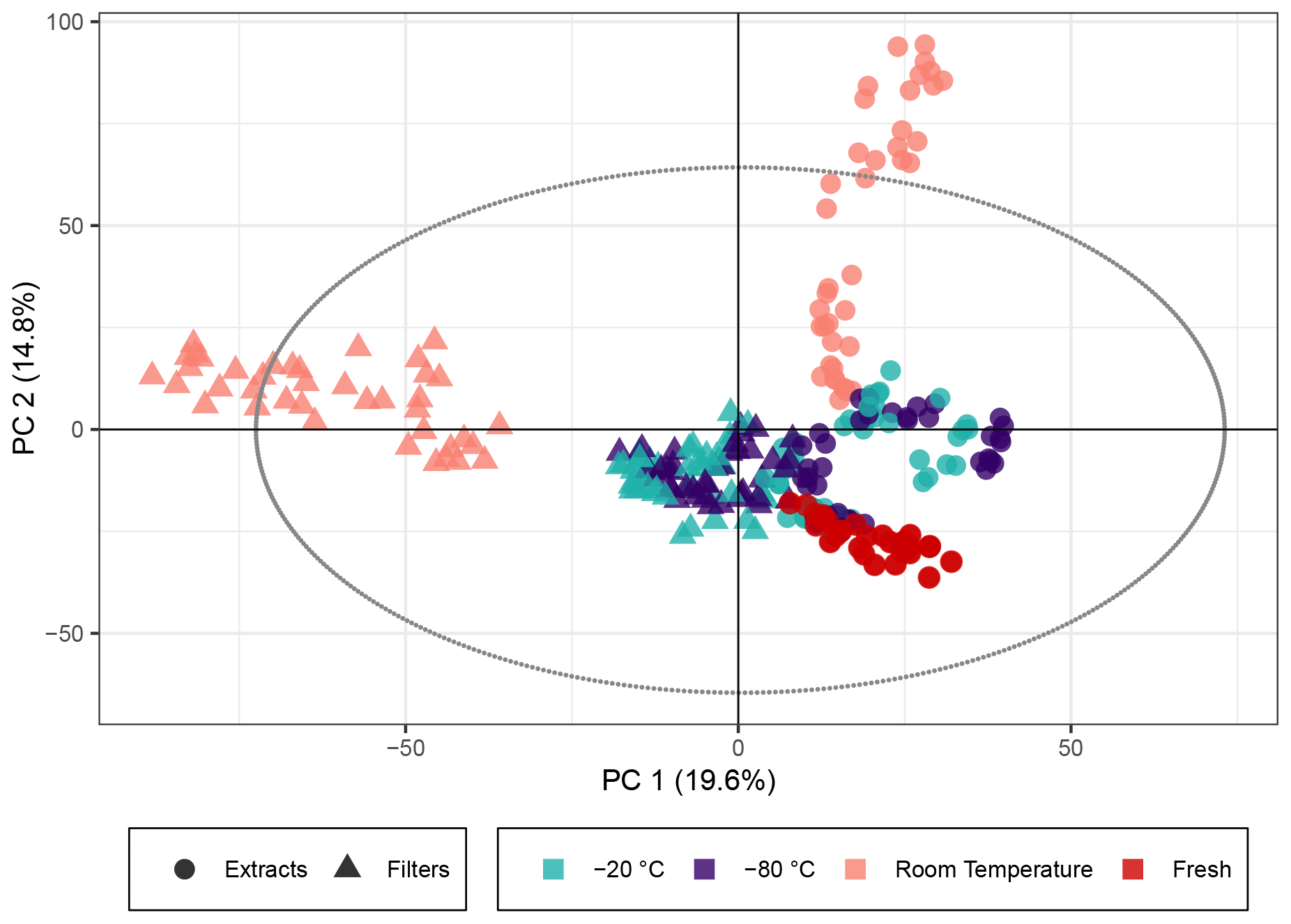
Figure 1PCA score plot of the β-pinene SOA samples. The colors represent the storage temperature, and the directly analyzed (i.e., fresh) samples and icons indicate the storage type. Hotelling's T2 ellipse (95 %) is represented by the dotted line. R2X[1] is 0.196, R2X[2] is 0.148, Q2[1] is 0.190, and Q2[2] is 0.176.
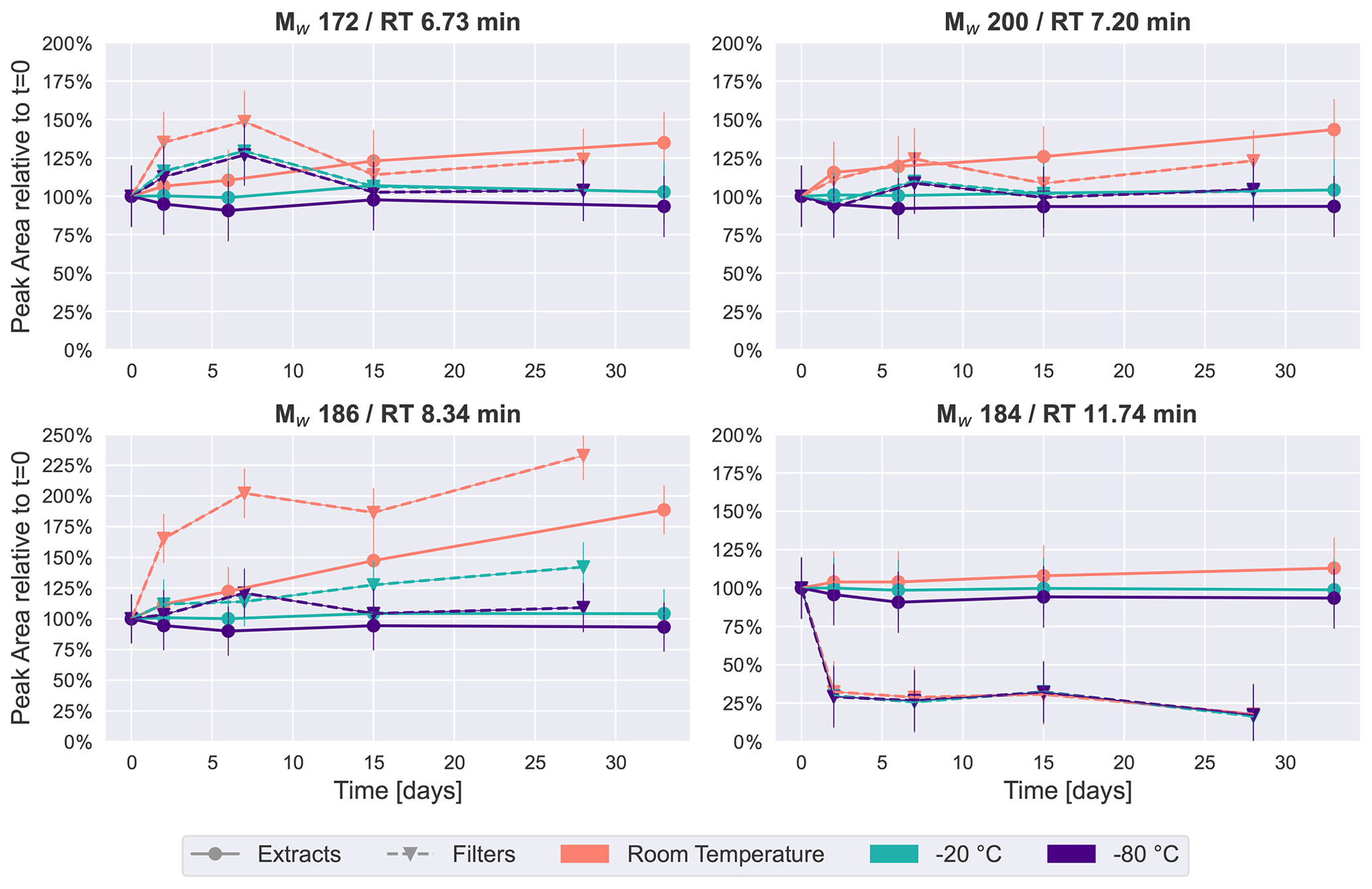
Figure 2Time series plots of the four most intense peaks in the β-pinene SOA samples over a period of 4–5 weeks. Especially for room temperature storage conditions, the concentration of some of these four compounds changes considerably.
In contrast, samples kept at room temperature drift away from the fresh samples in the PCA model, indicating a change in composition. Samples stored as filters or extracts at room temperature displayed a different behavior in PC1 and PC2 (PC1 giving the biggest variance for the filters and PC2 for the extracts). This suggests that there is a significant difference between samples that are extracted immediately and ones that are kept as filters at room temperature. For these room temperature samples, there is a clear temporal trend over the storage time of about 4 weeks: the longer the samples were kept at room temperature, the larger the deviation from the fresh samples (see also Fig. S2, displaying the storage time for each data point). Both the filters and the extracts stored at room temperature for 2 and 4 weeks surprisingly unveil signals outside of Hotelling's ellipse representing the 95 % limit of the multivariate probability distribution for the dataset, indicating that if the sample set was unknown, these samples might be qualified as outliers. The filters and extracts stored at room temperature seem to change their overall composition most significantly during the first days of storage because the biggest change per day seems to occur at the beginning of the storage time (Fig. S2).
The four most intense peaks in the base peak chromatogram (see Fig. S4) of the immediate extracts were chosen as representative of how the relative concentration of individual chromatographic peaks change over time under the different storage conditions. Figure 2 illustrates these temporal trends, sorted by retention time, where each point represents the average of two repeated analyses of each of the five filters collected (i.e., the average of 10 UHPLC–MS analyses). All four compounds or isomers of these have been identified in previous studies as carboxylic acids in SOA from gas-phase oxidation of α-pinene/β-pinene (Glasius et al., 2000; Yasmeen et al., 2010; Sato et al., 2016), and we tentatively confirmed the Mw 184 (detected as 183.1027, C10H15O3) peak at 11.74 min to be cis-pinonic acid through comparison with an authentic standard.
The time series plots show a similar trend to the PCA results: the samples kept at −20 or −80 ∘C demonstrated the highest stability, where peak areas are also mostly within 25 % of the values detected in the freshly analyzed samples for Mw 172 (detected as 171.0663, RT 6.73 min, C8H11O4), Mw 200 (detected as 199.0976, RT 7.20 min, C10H15O4) and Mw 186 (detected as 185.0819, RT 8.34 min, C9H13O4). This clearly indicates that storing the samples at −20 ∘C or below conserves samples sufficiently to prevent significant changes to these highest-intensity peaks.
In contrast, for features with Mw 172, 186 and 200, the extracts and filters at room temperature demonstrated noticeable increases over time (Fig. 2). This observation seems to contradict the hypothesis that compounds decay during storage. However, a possible explanation for this increase in these prominent features in the monomeric mass region might be a decomposition of oligomers (i.e., compounds with 11 or more carbon atoms). Since it is assumed there is limited oxidation chemistry occurring during storage, it is unlikely that the concentration of these compounds increased due to oxidation reactions, which is the dominant formation pathway of these compounds in the atmosphere. One class of oligomers frequently described in the literature is dimer esters (Hall and Johnston, 2012; Kenseth et al., 2018; Kristensen et al., 2016). The hydrolysis of dimer esters in samples stored in aqueous solution results in an increase in the intensity of the precursor monomers as decomposition products (i.e., compounds with 10 or fewer carbon atoms) (Zhao et al., 2018), which in our case would be the carboxylic acids discussed here. A time series analysis of the dimer ester Mw 388 (detected as 387.0759, C18H28O9) (Kristensen et al., 2016) is given in Fig. S5. This compound showed a clear decrease over time for samples stored as extracts at room temperature, and it might therefore be one of the compounds decaying in the sample, causing the observed concentration increase in compounds presented in Fig. 2.
An exception to this trend is cis-pinonic acid (Mw 184, RT 11.74 min), which had little temperature dependency, but the signal dropped by about 75 % for the samples which were kept on the filters, whereas it remained relatively stable in immediately extracted samples. Previous studies have observed similar results, where cis-pinonic acid demonstrated different behavior in comparison with the rest of the dataset, i.e., with a desorptive loss upon purging spiked filters with clean air (Glasius et al., 2000) or a decrease in acetonitrile and an increase in water over time (Wong et al., 2021).
Overall, the results for β-pinene SOA demonstrate that samples, both extracts and filters, kept at temperatures of −20 ∘C or below exhibited good stability of signal intensity over time, emphasizing that for studies conducting detailed offline analysis of SOA, composition samples should immediately be frozen after collection until analysis. However, these results also indicate that at least some compounds change over time, even under these low-temperature storage conditions, and the impacts of these artifacts on quantitative and compositional analyses must be considered. For samples kept at room temperature, there were clear and significant temporal changes in the signal intensity for many features as illustrated in Figs. 1 and 2, and samples stored for a day or longer at room temperature before analysis should not be considered for detailed chemical characterization.
3.2 Laboratory-generated SOA from naphthalene
Naphthalene SOA (a representative anthropogenic aerosol; Eiguren-Fernandez et al., 2004) samples were analyzed analogously to the β-pinene samples. A total of 5640 peaks with an intensity higher than 7×10⁵ (equivalent to 0.19 % of the highest intensity in the sample) were detected in 269 analyses. The PCA score plot for naphthalene SOA in Fig. 3 displayed similar overall trends using the non-normalized peak intensities as for β-pinene SOA (see Fig. 1). The generation of naphthalene SOA particles in the flow tube is slightly more unstable than for β-pinene; therefore the spread of fresh samples was higher across the five filter repeats as compared with the β-pinene samples. Similar to β-pinene SOA, the naphthalene samples kept frozen at −20 or at −80 ∘C exhibited closer profiles to the immediately analyzed samples and deviated little beyond the spread of the freshly extracted samples in the PCA model. For the room temperature samples there was a clear trend of variation associated with storage time for the extracts, which showed the largest variation in PC1, and for the filters, which showed the largest variation in PC2. This similarity with the β-pinene samples again indicates that the overall composition of the SOA samples stored for 2–4 weeks at room temperature deviated significantly from the immediately analyzed samples and that the influence of the extract and filter storage results in very different compositional changes. The samples kept at room temperature for 2–4 weeks fell outside Hotelling's T2 ellipse (see Fig. S6), again indicating that relative to the other samples, they have differing profiles and much larger variance across their features. The PCA score plot with log 10(x) normalized peak intensities is given in Fig. S7 and shows the same trends for all three temperatures as the score plot for the non-normalized peak intensities.
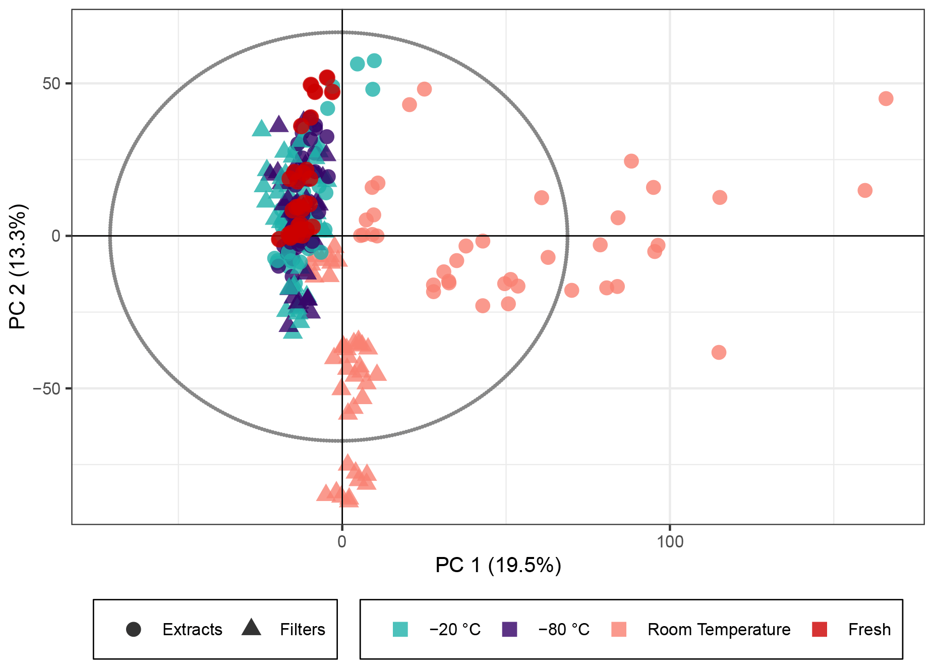
Figure 3PCA score plot of the naphthalene SOA samples. The colors represent the storage temperature, and the directly analyzed (i.e., fresh) samples and icons indicate the storage type. Hotelling's T2 ellipse (95 %) is represented by the dotted line. R2X[1] is 0.195, R2X[2] is 0.133, Q2[1] is 0.135, and Q2[2] is 0.153.
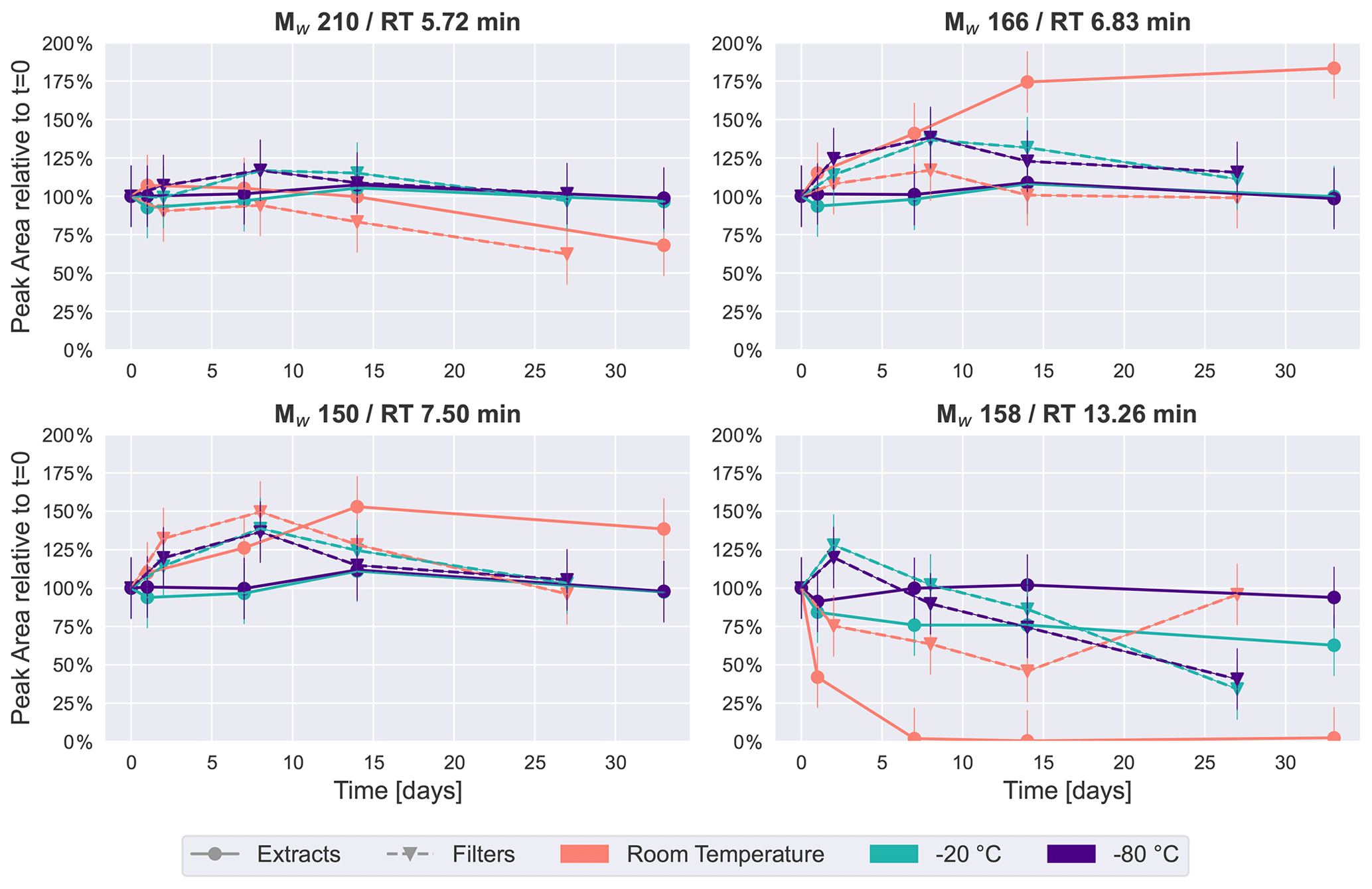
Figure 4Time series plots of the four most intense peaks in the naphthalene SOA samples. Similar to β-pinene SOA (Fig. 2), room temperature storage significantly affects the concentration of some compounds in naphthalene SOA.
These trends were also visible for the four most intense peaks in the base peak chromatogram of naphthalene SOA samples as presented in Fig. 4. Again, the most stable storage conditions were freezing of the samples, and extracted samples indicated a slightly improved temporal stability over the samples stored on filters in the freezers. The most noticeable changes occurred for samples kept at room temperature. The most significant decay over time at room temperature was seen for Mw 158 (detected protonated anion of Mw 158: 159.0451, C10H7O2) at 13.26 min, which was identified as 1,2-naphthoquinone through comparison with an authentic standard. For extracts, the signal intensity dropped to less than half in the first 24 h, before disappearing completely in the samples analyzed after 1–4 weeks, and it appeared stable only when stored at −80 ∘C as the extract. 1,2-Naphthoquinone is of increasing interest in the literature, as oxidized polycyclic aromatic hydrocarbons (PAHs) are known to cause oxidative stress in human lung cells and are thus a direct contributor to particle toxicity from anthropogenic sources (Kelly, 2003). It is evident from this data that particle extraction and storage conditions need to be carefully described and considered when these compounds are used for source apportionment or to infer particle health effects from laboratory-generated samples.
Mw 166 (detected as 165.0192, RT 6.83 min, C8H5O4) has previously been found in naphthalene SOA samples and identified as phthalic acid (Kleindienst et al., 2012). The most stable conditions for this compound were again observed when samples were kept frozen, while in extracts stored at room temperature, this compound steadily increased to almost double the intensity after a month. A possible explanation for the increase in especially Mw 166 could again be the decay of oligomeric compounds, causing an increase in their monomeric counterparts.
The other isomers of Mw 210 (detected as 209.0455, RT 5.72 min, C10H9O5) and Mw 150 (detected as 149.0243, RT 7.50 min, C8H5O3) selected for Fig. 4 showed moderate changes in comparison with the previously discussed compounds. Both exhibited relatively little change over time in samples which were kept in the freezers. The largest time-related effect can be seen for the samples kept at room temperature, where there is either a decrease (Mw 210) or an increase (Mw 150) of around 40 % after 4 weeks.
These four most intense peaks contributed the most to the variance observed in the PCA score plots, thus driving the separation of samples by storage condition, and again reinforce the requirement to store organic aerosol samples in a freezer to best preserve their original composition.
3.3 Atmospheric aerosol
To assess if the significant temporal trends and the differences in storage (i.e., filter vs. extracts) observed for laboratory-generated SOA samples were also visible in ambient samples, we collected five high-volume ambient aerosol samples in the city center of Basel and analyzed, extracted and stored them using the same methods as for the laboratory-generated SOA samples.
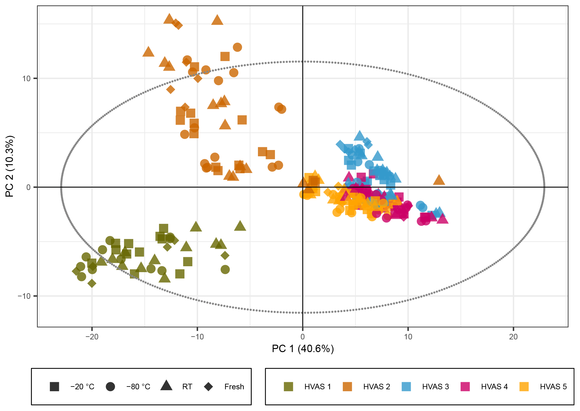
Figure 5PCA score plot representing the HVAS filters with the exclusion of the batch effect due to different mobile phases. The colors represent the different HVAS filters and shapes the different storage temperatures. R2X[1] is 0.406, R2X[2] is 0.103, Q2[1] is 0.399, and Q2[2] is 0.157.
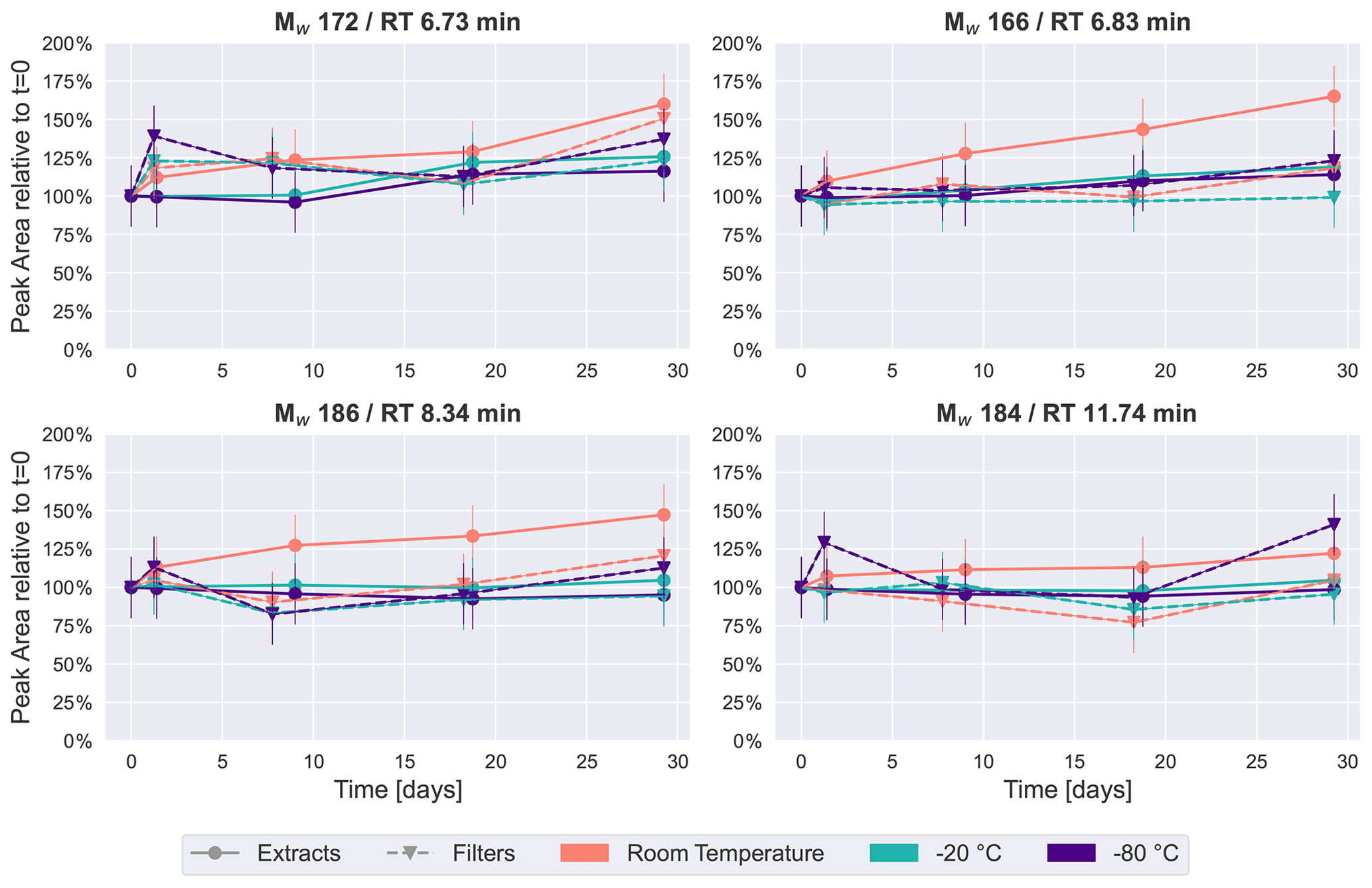
Figure 6Time series of an average of 2–5 HVASs of four previously detected peaks in the SOA samples from β-pinene ( 171.0663, 185.0819 and 183.1027) and from naphthalene ( 165.0192).
The PCA score plot with non-normalized peak intensities for the ambient samples is given in Fig. 5 (the score plots with log 10(x) normalized peak intensities are given in Figs. S9 and S11, showing the same trends). The colors represent the five different HVASs, and shapes correspond to storage temperatures. More detailed information on storage temperature and type is given in separate score plots in the Supplement (Figs. S8 and S10). During LC–MS analysis of the ambient samples, a different batch of UHPLC-grade water from the supplier was needed for the samples stored for 3–4 weeks, causing higher background signals and a reduced overall signal intensity for peaks with lower intensities. This difference in signal intensity could be adjusted in the time series analysis of the compounds previously detected in SOA samples through the intensity of our standard mix but was difficult to account for in the PCA. In order to solve this problem, the peak intensity parameter was increased from 7×10⁵ (as used for the SOA samples discussed above) to 4×10⁶ (equivalent to 4 % of the highest peak intensity in the sample) to reduce the number of total compounds detected from 2800 to around 400 because the higher intensity peaks were not significantly affected by this increased background. Additionally, a time series of the signal intensity of individual compounds was checked manually to exclude compounds which had a clear “step function”, leaving roughly 240 compounds to be included in the PCA. The non-corrected version of the score plot is given in Fig. S12, where the same general trend is still visible as in Figs. 5, S8 and S10.
In strong contrast to the laboratory-generated SOA samples, the PCA score plots for the ambient samples indicated little storage-dependent variation in the signals, as samples grouped together in the first two PCs independently of storage temperature or condition, indicating a much larger influence of individual samples on the variance than of the storage condition. The HVASs from days 3–5 showed similar scores, as they were all sampled in the same week or even on consecutive days. To ensure that there was no additional variation between the storage temperatures, we also looked at PCA score plots of the individual HVASs, which presented the same trends (data not shown).
We conclude that in ambient samples the concentration of organic components is overall more stable over time and is apparently less affected by storage conditions compared with laboratory-generated SOA samples. This could be due to several factors. Organic components in ambient particles originate not only from SOA sources but include many primary particle components from other sources such as biomass burning, fossil fuel combustion, industrial activities (e.g., solvents) and primary biological material (Seinfeld and Pankow, 2003). Components from these sources might be more stable than SOA components. In addition, in ambient samples, a significant fraction of the total particle mass is inorganic components (mainly ions like sulfate, nitrate and ammonium), resulting in a more diluted concentration of individual organic components (compared with pure laboratory-generated SOA samples), which might limit the availability of organic reaction partners, and thus increasing the stability of some organic components.
For a compound-specific comparison between SOA and ambient samples, we analyzed four compounds which were detected in all HVASs, and which were also among the four highest peaks in the SOA samples (see Figs. 2 and 4). The time series for these compounds in the HVASs is given in Fig. 6. HVAS 1 was excluded from this analysis because of the missing 2-week time point (Table S2). Overall, these compounds were more stable over time in the ambient samples compared with the pure SOA samples, as also indicated in the PCA analysis, supporting the hypothesis that the lower concentrations of individual organic compounds in ambient aerosol lead to less signal change over time. This increased stability might also be due to the lower oligomer content in ambient aerosol in comparison with laboratory-generated SOA (Kourtchev et al., 2016). Nevertheless, clear changes were observed for Mw 166 and 186 for samples stored at room temperature and as extracts, which showed similar patterns to ambient and pure SOA samples. Slight changes over time (especially after 4 weeks) were seen for the Mw 172 feature in the room temperature samples. The largest difference between ambient and laboratory SOA samples was observed for cis-pinonic acid (Mw 184), where there was no significant difference between filter and extract storage in the ambient samples, but a large decay occurred in the pure SOA samples stored on filters. Reasons for this very different behavior are unknown but could be related to the different filter material used for ambient and lab samples (quartz vs. PTFE). Another cause could be desorptive loss of cis-pinonic acid due to the large air masses in the HVAS as previously reported (Glasius et al., 2000).
Overall, the storage of ambient samples on filters demonstrates very good stability of the signal intensity and provides confidence that the concentration of organic components may not change significantly in ambient urban samples which are collected weeks before analysis and which are stored on filters.
The results in this study represent a thorough investigation of the temporal changes in the detailed organic composition of offline aerosol samples collected on filters under different storage conditions and for different types of aerosol. Both SOA and ambient samples largely preserved their chemical profiles when stored at temperatures of −20 or −80 ∘C for up to 4–6 weeks. We could clearly demonstrate that there was no discernible difference in the particle composition when particles were stored at −20 or at −80 ∘C, with the exception of very few individual components such as cis-pinonic acid (Fig. 2) and extracts stored for extended periods of time (i.e., ≥4 weeks) when the lower-intensity features are weighted more (as illustrated in Fig. S3).
However, for all investigated samples, but especially for laboratory-generated samples, storage of filters and of extracts at room temperature significantly affected the concentration of individual organic components, where compound formation as well as decomposition were observed. Many compounds with a high signal intensity in the chromatogram exhibited a significant increase in concentration over time when they were stored at room temperature. A possible explanation for this observation could be that some of these compounds are formed in the samples via decay of oligomers during storage, leading to an increase in their respective monomers. The different temporal behaviors of room temperature extracts and filters (as seen in Figs. 1 and 3) could be explained by the hydrolysis of components in the aqueous extracts versus continuing reactions of components in the organic matrix on the filters. Keeping the samples frozen between collection and analysis appeared to largely avoid such decomposition reactions.
In many previous studies, the time between sampling and analysis is at least a few days, potentially up to many years, and often storage conditions are only poorly described in publications. The study presented here evidently indicates that careful storage procedures should be adopted and described in detail in publications in order to assess potential distortions of the original particle composition, especially for laboratory or atmospheric simulation chamber samples, where significant changes can occur within a day after particle generation.
These compositional changes seemed to be less problematic for ambient particles at the urban site characterized here, but for some compounds the concentration changed by 50 % or more in ambient samples when analyzed several weeks after collection. Thus, when concentrations of individual organic particle components are studied in detail, a careful evaluation of their stability before analysis is demonstrably important, especially when samples are kept for days or weeks at room temperature, for example during automated filter sampling. In samples from other locations, e.g., remote sites, with higher or even dominant SOA contributions, the stability could be less favorable than for the urban samples analyzed here and could resemble the laboratory-generated SOA samples analyzed in this study more.
Recommendations for future studies, when organic molecular-level composition analyses are performed, are that all samples should be kept frozen (−20 ∘C) as soon as possible after sampling, i.e., within a few hours, to avoid significant compositional changes. If this is not feasible, authors should mention in detail how the samples were stored and how much time passed between collection and analysis.
All code and data used are available upon request from the corresponding author.
The supplement related to this article is available online at: https://doi.org/10.5194/acp-23-9161-2023-supplement.
JR, KW and MK designed the study. AB generated and collected the laboratory-generated SOA samples. JR collected the ambient aerosol samples and performed all other experimental and data analysis work. JR wrote the paper with contributions from all co-authors.
The contact author has declared that none of the authors has any competing interests.
Publisher’s note: Copernicus Publications remains neutral with regard to jurisdictional claims in published maps and institutional affiliations.
This research has been supported by the Schweizerischer Nationalfonds zur Förderung der Wissenschaftlichen Forschung (grant no. 200021_192192/1).
This paper was edited by Theodora Nah and reviewed by three anonymous referees.
Benton, H. P., Want, E. J., and Ebbels, T. M. D.: Correction of mass calibration gaps in liquid chromatography-mass spectrometry metabolomics data, Bioinformatics, 26, 2488–2489, https://doi.org/10.1093/bioinformatics/btq441, 2010.
CEN, European Committee for Standardization: EN 12341:2014 Ambient air – Standard gravimetric measurement method for the determination of the PM10 or PM2.5 mass concentration of suspended particulate matter, CEN-CENELEC, 2014.
Chambers, M. C., MacLean, B., Burke, R., Amodei, D., Ruderman, D. L., Neumann, S., Gatto, L., Fischer, B., Pratt, B., Egertson, J., Hoff, K., Kessner, D., Tasman, N., Shulman, N., Frewen, B., Baker, T. A., Brusniak, M. Y., Paulse, C., Creasy, D., Flashner, L., Kani, K., Moulding, C., Seymour, S. L., Nuwaysir, L. M., Lefebvre, B., Kuhlmann, F., Roark, J., Rainer, P., Detlev, S., Hemenway, T., Huhmer, A., Langridge, J., Connolly, B., Chadick, T., Holly, K., Eckels, J., Deutsch, E. W., Moritz, R. L., Katz, J. E., Agus, D. B., MacCoss, M., Tabb, D. L., and Mallick, P.: A cross-platform toolkit for mass spectrometry and proteomics, Nat. Biotechnol., 30, 918–920, https://doi.org/10.1038/nbt.2377, 2012.
Dillner, A. M., Phuah, C. H., and Turner, J. R.: Effects of post-sampling conditions on ambient carbon aerosol filter measurements, Atmos. Environ., 43, 5937–5943, https://doi.org/10.1016/j.atmosenv.2009.08.009, 2009.
Eiguren-Fernandez, A., Miguel, A. H., Froines, J. R., Thurairatnam, S., and Avol, E. L.: Seasonal and spatial variation of polycyclic aromatic hydrocarbons in vapor-phase and PM2.5 in Southern California urban and rural communities, Aerosol Sci. Tech., 38, 447–455, https://doi.org/10.1080/02786820490449511, 2004.
Fuller, S. J., Wragg, F. P. H., Nutter, J., and Kalberer, M.: Comparison of on-line and off-line methods to quantify reactive oxygen species (ROS) in atmospheric aerosols, Atmos. Environ., 92, 97–103, https://doi.org/10.1016/j.atmosenv.2014.04.006, 2014.
Glasius, M., Lahaniati, M., Calogirou, A., Di Bella, D., Jensen, N. R., Hjorth, J., Kotzias, D., and Larsen, B. R.: Carboxylic acids in secondary aerosols from oxidation of cyclic monoterpenes by ozone, Environ. Sci. Technol., 34, 1001–1010, https://doi.org/10.1021/es990445r, 2000.
Hall, W. A. and Johnston, M. V.: Oligomer formation pathways in secondary organic aerosol from MS and MS/MS measurements with high mass accuracy and resolving power, J. Am. Soc. Mass Spectrom., 23, 1097–1108, https://doi.org/10.1007/s13361-012-0362-6, 2012.
Hallquist, M., Wenger, J. C., Baltensperger, U., Rudich, Y., Simpson, D., Claeys, M., Dommen, J., Donahue, N. M., George, C., Goldstein, A. H., Hamilton, J. F., Herrmann, H., Hoffmann, T., Iinuma, Y., Jang, M., Jenkin, M. E., Jimenez, J. L., Kiendler-Scharr, A., Maenhaut, W., McFiggans, G., Mentel, Th. F., Monod, A., Prévôt, A. S. H., Seinfeld, J. H., Surratt, J. D., Szmigielski, R., and Wildt, J.: The formation, properties and impact of secondary organic aerosol: current and emerging issues, Atmos. Chem. Phys., 9, 5155–5236, https://doi.org/10.5194/acp-9-5155-2009, 2009.
Harris, C. R., Millman, K. J., van der Walt, S. J., Gommers, R., Virtanen, P., Cournapeau, D., Wieser, E., Taylor, J., Berg, S., Smith, N. J., Kern, R., Picus, M., Hoyer, S., van Kerkwijk, M. H., Brett, M., Haldane, A., del Río, J. F., Wiebe, M., Peterson, P., Gérard-Marchant, P., Sheppard, K., Reddy, T., Weckesser, W., Abbasi, H., Gohlke, C., and Oliphant, T. E.: Array programming with NumPy, Nature, 585, 357–362, https://doi.org/10.1038/s41586-020-2649-2, 2020.
Hunter, J. D.: Matplotlib: A 2D Graphics Environment, Comput. Sci. Eng., 9, 90–95, https://doi.org/10.1109/MCSE.2007.55, 2007.
Jimenez, J. L., Canagaratna, M. R., Donahue, N. M., Prevot, A. S. H., Zhang, Q., Kroll, J. H., DeCarlo, P. F., Allan, J. D., Coe, H., Ng, N. L., Aiken, A. C., Docherty, K. S., Ulbrich, I. M., Grieshop, A. P., Robinson, A. L., Duplissy, J., Smith, J. D., Wilson, K. R., Lanz, V. A., Hueglin, C., Sun, Y. L., Tian, J., Laaksonen, A., Raatikainen, T., Rautiainen, J., Vaattovaara, P., Ehn, M., Kulmala, M., Tomlinson, J. M., Collins, D. R., Cubison, M. J., Dunlea, E. J., Huffman, J. A., Onasch, T. B., Alfarra, M. R., Williams, P. I., Bower, K., Kondo, Y., Schneider, J., Drewnick, F., Borrmann, S., Weimer, S., Demerjian, K., Salcedo, D., Cottrell, L., Griffin, R., Takami, A., Miyoshi, T., Hatakeyama, S., Shimono, A., Sun, J. Y., Zhang, Y. M., Dzepina, K., Kimmel, J. R., Sueper, D., Jayne, J. T., Herndon, S. C., Trimborn, A. M., Williams, L. R., Wood, E. C., Middlebrook, A. M., Kolb, C. E., Baltensperger, U., and Worsnop, D. R.: Evolution of organic aerosols in the atmosphere, Science, 326, 1525–1529, https://doi.org/10.1126/science.1180353, 2009.
Johnston, M. V. and Kerecman, D. E.: Molecular Characterization of Atmospheric Organic Aerosol by Mass Spectrometry, Annu. Rev. Anal. Chem., 12, 247–274, https://doi.org/10.1146/annurev-anchem-061516-045135, 2019.
Keller, A., Kalbermatter, D. M., Wolfer, K., Specht, P., Steigmeier, P., Resch, J., Kalberer, M., Hammer, T., and Vasilatou, K.: The organic coating unit, an all-in-one system for reproducible generation of secondary organic matter aerosol, Aerosol Sci. Tech., 56, 947–958, https://doi.org/10.1080/02786826.2022.2110448, 2022.
Kelly, F. J.: Oxidative stress: Its role in air pollution and adverse health effects, Occup. Environ. Med., 60, 612–616, https://doi.org/10.1136/oem.60.8.612, 2003.
Kenseth, C. M., Huang, Y., Zhao, R., Dalleska, N. F., Caleb Hethcox, J., Stoltz, B. M., and Seinfeld, J. H.: Synergistic O3 + OH oxidation pathway to extremely low-volatility dimers revealed in β-pinene secondary organic aerosol, P. Natl. Acad. Sci. USA, 115, 8301–8306, https://doi.org/10.1073/pnas.1804671115, 2018.
Kleindienst, T. E., Jaoui, M., Lewandowski, M., Offenberg, J. H., and Docherty, K. S.: The formation of SOA and chemical tracer compounds from the photooxidation of naphthalene and its methyl analogs in the presence and absence of nitrogen oxides, Atmos. Chem. Phys., 12, 8711–8726, https://doi.org/10.5194/acp-12-8711-2012, 2012.
Kourtchev, I., Giorio, C., Manninen, A., Wilson, E., Mahon, B., Aalto, J., Kajos, M., Venables, D., Ruuskanen, T., Levula, J., Loponen, M., Connors, S., Harris, N., Zhao, D., Kiendler-Scharr, A., Mentel, T., Rudich, Y., Hallquist, M., Doussin, J. F., Maenhaut, W., Bäck, J., Petäjä, T., Wenger, J., Kulmala, M., and Kalberer, M.: Enhanced volatile organic compounds emissions and organic aerosol mass increase the oligomer content of atmospheric aerosols, Sci. Rep., 6, 1–9, https://doi.org/10.1038/srep35038, 2016.
Kristensen, K., Watne, Å. K., Hammes, J., Lutz, A., Petäjä, T., Hallquist, M., Bilde, M., and Glasius, M.: High-Molecular Weight Dimer Esters Are Major Products in Aerosols from α-Pinene Ozonolysis and the Boreal Forest, Environ. Sci. Tech. Let., 3, 280–285, https://doi.org/10.1021/acs.estlett.6b00152, 2016.
Mark, G., Tauber, A., Laupert, R., Schuchmann, H. P., Schulz, D., Mues, A., and Von Sonntag, C.: OH-radical formation by ultrasound in aqueous solution – Part II: Terephthalate and Fricke dosimetry and the influence of various conditions on the sonolytic yield, Ultrason. Sonochem., 5, 41–52, https://doi.org/10.1016/S1350-4177(98)00012-1, 1998.
NABEL: Technischer Bericht zum Nationalen Beobachtungsnetz für Luftfremdstoffe (NABEL), 209 pp., https://www.bafu.admin.ch/bafu/de/home/themen/luft/zustand/daten/nationales-beobachtungsnetz-fuer-luftfremdstoffe--nabel-.html (last access: 17 August 2023), 2023.
Nozière, B., Kalberer, M., Claeys, M., Allan, J., D'Anna, B., Decesari, S., Finessi, E., Glasius, M., Grgić, I., Hamilton, J. F., Hoffmann, T., Iinuma, Y., Jaoui, M., Kahnt, A., Kampf, C. J., Kourtchev, I., Maenhaut, W., Marsden, N., Saarikoski, S., Schnelle-Kreis, J., Surratt, J. D., Szidat, S., Szmigielski, R., and Wisthaler, A.: The Molecular Identification of Organic Compounds in the Atmosphere: State of the Art and Challenges, Chem. Rev., 115, 3919–3983, https://doi.org/10.1021/cr5003485, 2015.
Parshintsev, J., Ruiz-Jimenez, J., Petäjä, T., Hartonen, K., Kulmala, M., and Riekkola, M. L.: Comparison of quartz and Teflon filters for simultaneous collection of size-separated ultrafine aerosol particles and gas-phase zero samples, Anal. Bioanal. Chem., 400, 3527–3535, https://doi.org/10.1007/s00216-011-5041-0, 2011.
Pereira, K. L., Ward, M. W., Wilkinson, J. L., Sallach, J. B., Bryant, D. J., Dixon, W. J., Hamilton, J. F., and Lewis, A. C.: An Automated Methodology for Non-targeted Compositional Analysis of Small Molecules in High Complexity Environmental Matrices Using Coupled Ultra Performance Liquid Chromatography Orbitrap Mass Spectrometry, Environ. Sci. Technol., 55, 7365–7375, https://doi.org/10.1021/acs.est.0c08208, 2021.
Perrino, C., Canepari, S., and Catrambone, M.: Comparing the performance of Teflon and quartz membrane filters collecting atmospheric PM: Influence of atmospheric water, Aerosol Air Qual. Res., 13, 137–147, https://doi.org/10.4209/aaqr.2012.07.0167, 2013.
Pöschl, U. and Shiraiwa, M.: Multiphase Chemistry at the Atmosphere-Biosphere Interface Influencing Climate and Public Health in the Anthropocene, Chem. Rev., 115, 4440–4475, https://doi.org/10.1021/cr500487s, 2015.
Raybaut, P.: Spyder-documentation, http://pythonhosted.org (last access: 17 August 2023), 2009.
Roper, C., Delgado, L. S., Barrett, D., Massey Simonich, S. L., and Tanguay, R. L.: PM2.5 Filter Extraction Methods: Implications for Chemical and Toxicological Analyses, Environ. Sci. Technol., 53, 434–442, https://doi.org/10.1021/acs.est.8b04308, 2019.
Sato, K., Jia, T., Tanabe, K., Morino, Y., Kajii, Y., and Imamura, T.: Terpenylic acid and nine-carbon multifunctional compounds formed during the aging of β-pinene ozonolysis secondary organic aerosol, Atmos. Environ., 130, 127–135, https://doi.org/10.1016/j.atmosenv.2015.08.047, 2016.
Seinfeld, J. H. and Pankow, J. F.: Organic Atmospheric Particulate Material, Annu. Rev. Phys. Chem., 54, 121–140, https://doi.org/10.1146/annurev.physchem.54.011002.103756, 2003.
Smith, C. A., Want, E. J., O'Maille, G., Abagyan, R., and Siuzdak, G.: XCMS: Processing mass spectrometry data for metabolite profiling using nonlinear peak alignment, matching, and identification, Anal. Chem., 78, 779–787, https://doi.org/10.1021/ac051437y, 2006.
Stark, H., Yatavelli, R. L. N., Thompson, S. L., Kimmel, J. R., Cubison, M. J., Chhabra, P. S., Canagaratna, M. R., Jayne, J. T., Worsnop, D. R., and Jimenez, J. L.: Methods to extract molecular and bulk chemical information from series of complex mass spectra with limited mass resolution, Int. J. Mass Spectrom., 389, 26–38, https://doi.org/10.1016/j.ijms.2015.08.011, 2015.
Tautenhahn, R., Bottcher, C., and Neumann, S.: Highly sensitive feature detection for high resolution LC/MS, BMC Bioinformatics, 9, 1–16, https://doi.org/10.1186/1471-2105-9-504, 2008.
Van Rossum, G. and Drake, F. L.: Python 3 Reference Manual, CreateSpace, Scotts Valley, CA, ISBN 1441412697, 2009.
Wickham, H.: ggplot2: Elegant Graphics for Data Analysis, Springer-Verlag New York, 260 pp., https://doi.org/10.1007/978-3-319-24277-4, 2016.
Wolfer, A. M., Correia, G. D. S., Sands, C. J., Camuzeaux, S., Yuen, A. H. Y., Chekmeneva, E., Takáts, Z., Pearce, J. T. M., and Lewis, M. R.: peakPantheR, an R package for large-scale targeted extraction and integration of annotated metabolic features in LC–MS profiling datasets, Bioinformatics, 37, 4886–4888, https://doi.org/10.1093/bioinformatics/btab433, 2021.
Wong, C., Vite, D., and Nizkorodov, S. A.: Stability of α-Pinene and d-Limonene Ozonolysis Secondary Organic Aerosol Compounds Toward Hydrolysis and Hydration, ACS Earth Sp. Chem., 5, 2555–2564, https://doi.org/10.1021/acsearthspacechem.1c00171, 2021.
Yasmeen, F., Vermeylen, R., Szmigielski, R., Iinuma, Y., Böge, O., Herrmann, H., Maenhaut, W., and Claeys, M.: Terpenylic acid and related compounds: precursors for dimers in secondary organic aerosol from the ozonolysis of α- and β-pinene, Atmos. Chem. Phys., 10, 9383–9392, https://doi.org/10.5194/acp-10-9383-2010, 2010.
Zhao, R., Kenseth, C. M., Huang, Y., Dalleska, N. F., Kuang, X. M., Chen, J., Paulson, S. E., and Seinfeld, J. H.: Rapid Aqueous-Phase Hydrolysis of Ester Hydroperoxides Arising from Criegee Intermediates and Organic Acids, J. Phys. Chem. A, 122, 5190–5201, https://doi.org/10.1021/acs.jpca.8b02195, 2018.