Automated detection and monitoring of methane super-emitters using satellite data

A reduction in anthropogenic methane emissions is vital to limit near-term global warming. A small number of so-called super-emitters is responsible for a disproportionally large fraction of total methane emissions. Since late 2017, the TROPOspheric Monitoring Instrument (TROPOMI) has been in orbit, providing daily global coverage of methane mixing ratios at a resolution of up to 7×5.5 km², enabling the detection of these super-emitters. However, TROPOMI produces millions of observations each day, which together with the complexity of the methane data, makes manual inspection infeasible. We have therefore designed a two-step machine learning approach using a convolutional neural network to detect plume-like structures in the methane data and subsequently apply a support vector classifier to distinguish the emission plumes from retrieval artifacts. The models are trained on pre-2021 data and subsequently applied to all 2021 observations. We detect 2974 plumes in 2021, with a mean estimated source rate of 44 t h⁻¹ and 5–95th percentile range of 8–122 t h⁻¹. These emissions originate from 94 persistent emission clusters and hundreds of transient sources. Based on bottom-up emission inventories, we find that most detected plumes are related to urban areas and/or landfills (35 %), followed by plumes from gas infrastructure (24 %), oil infrastructure (21 %), and coal mines (20 %). For 12 (clusters of) TROPOMI detections, we tip and cue the targeted observations and analysis of high-resolution satellite instruments to identify the exact sources responsible for these plumes. Using high-resolution observations from GHGSat, PRISMA, and Sentinel-2, we detect and analyze both persistent and transient facility-level emissions underlying the TROPOMI detections. We find emissions from landfills and fossil fuel exploitation facilities, and for the latter, we find up to 10 facilities contributing to one TROPOMI detection. Our automated TROPOMI-based monitoring system in combination with high-resolution satellite data allows for the detection, precise identification, and monitoring of these methane super-emitters, which is essential for mitigating their emissions.

1 Introduction

Anthropogenic methane emissions have caused at least 25 % of human-induced global warming (Ocko et al., 2018; IPCC, 2021). Methane's atmospheric concentration has increased by a factor of 2.5 since the pre-industrialized era (Szopa et al., 2021), and the rate of increase has accelerated in recent years (NOAA, 2022). Due to its relatively short atmospheric lifetime and large global warming potential (81 times that of CO₂ over a time span of 20 years (IPCC, 2021)), methane has an important role in the rate of climate warming (Nisbet et al., 2020; Ocko et al., 2021; Szopa et al., 2021). Reducing global methane emissions is therefore vital to achieve the goals set out in the 2015 Paris Climate Accords (Nisbet et al., 2020). Since November 2021, over 125 countries have signed the Global Methane Pledge (European Commission, 2021; CCAC, 2022) and committed to reducing their methane emissions by 30 % in 2030 compared to 2020 levels. This could help avoid 0.2 ^∘C of global mean warming by 2050 (CCAC, 2022; UNEP and CCAC, 2021). In order to reduce global methane emissions fast and effectively during this decade, it is paramount to identify the largest anthropogenic sources of methane and mitigate those. We therefore propose an automated detection and monitoring system using satellite data with machine learning models to detect methane super-emitters.

The dominant anthropogenic methane emission sources are agriculture (livestock and rice cultivation), oil and gas exploitation, waste management, and coal mining; the exact locations and magnitudes of emissions are still uncertain (Saunois et al., 2020). Large fractions of methane emissions in various sectors could be mitigated using existing technology, with about a quarter of those at no net cost (Nisbet et al., 2020; Ocko et al., 2021; Lauvaux et al., 2022). Moreover, a small number of emitters is responsible for a disproportionally large fraction of total anthropogenic emissions (Zavala-Araiza et al., 2015; Jacob et al., 2016). These concentrated point sources are often referred to as “super-emitters” and are difficult to account for in global bottom-up inventories (Zavala-Araiza et al., 2015), as they are often caused by severe malfunctioning or abnormal operating conditions, e.g., dysfunctional natural gas flaring systems (Irakulis-Loitxate et al., 2022a, b; Plant et al., 2022). Super-emitters are not limited to oil and gas production and also occur in the coal mining and waste sectors (Cusworth et al., 2020; Sadavarte et al., 2021; Maasakkers et al., 2022b). Detection, localization, and global monitoring of these methane super-emitters provides a large opportunity to reduce emissions (UNEP and CCAC, 2021; Parry et al., 2022).

One way to obtain more insight with respect to where super-emitters occur is to perform measurements on the ground, with drones, or with aircraft campaigns. Several regions with known frequent and large methane emissions have been mapped in detail with aircraft campaigns (e.g., Frankenberg et al., 2016; Duren et al., 2019; Yu et al., 2022; Plant et al., 2022). While ground-based or airborne measurements are limited in spatial and temporal coverage, satellite observations have the potential for global monitoring of methane point sources with frequent revisits (Jacob et al., 2016; Cusworth et al., 2019; Jacob et al., 2022). The TROPOspheric Monitoring Instrument (TROPOMI) (Veefkind et al., 2012) was launched in 2017 and observes atmospheric dry-air methane column mixing ratios $X_{{\mathrm{CH}}_{\mathrm{4}}}$ with a pixel size down to 7 km × 5.5 km and daily global coverage (Hu et al., 2018; Lorente et al., 2021), resulting in a point source detection limit down to ∼5 t h⁻¹ under favorable conditions (Jacob et al., 2016). TROPOMI data have been used to quantify global- (Qu et al., 2021) and country-level (Chen et al., 2022) distributions of methane emissions and large area sources, such as oil and gas basins like the Permian Basin (Zhang et al., 2020; de Gouw et al., 2020; Schneising et al., 2020; Shen et al., 2022). Lauvaux et al. (2022) performed a study into oil- and gas-related methane super-emitters using TROPOMI data. Several individual super-emitters have been studied in detail using TROPOMI $X_{{\mathrm{CH}}_{\mathrm{4}}}$ data, including natural gas well blowouts (Pandey et al., 2019; Cusworth et al., 2021; Maasakkers et al., 2022a) and various persistent sources (Varon et al., 2019; Sadavarte et al., 2021; Tu et al., 2022a, b).

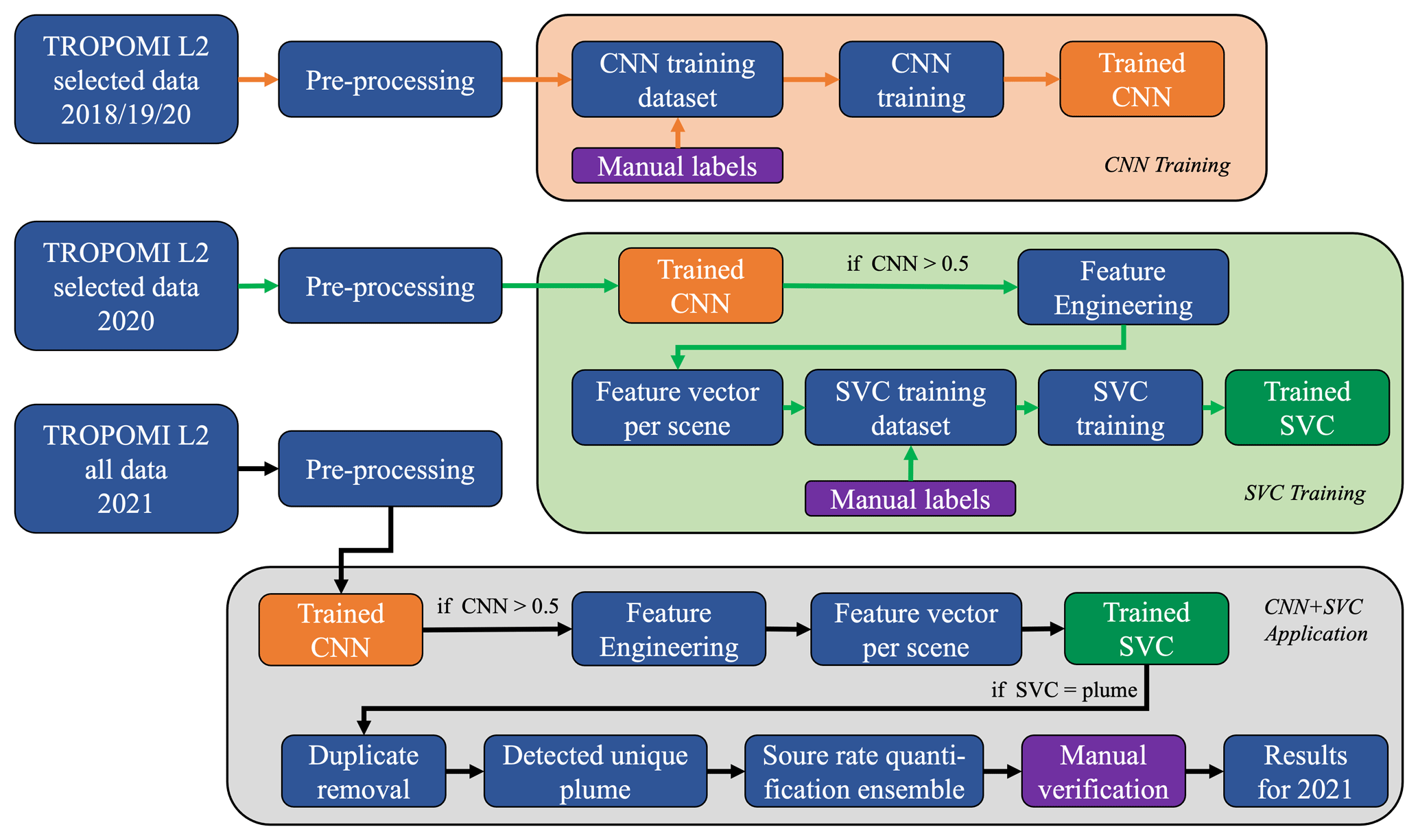
Figure 1 Flowchart showing the employed methodological framework. It consists of three phases, where each next phase uses the output (the trained model) of the previous phase, as indicated with matching colors (orange and green). We use the TROPOMI $X_{{\mathrm{CH}}_{\mathrm{4}}}$ Level 2 scientific data product version 18_17. Pre-processing is equivalent for each of the three phases and consists of filtering, destriping the $X_{{\mathrm{CH}}_{\mathrm{4}}}$ channel, and splitting up the data into 32×32 scenes. The output of the pre-processing is a dataset of [N, M, 32, 32], where N is the number of scenes, M is the number of channels (fields of data used later on; for example, the methane concentrations) and 32×32 gives the (pixel) dimensions of the scene. The CNN exclusively uses the $X_{{\mathrm{CH}}_{\mathrm{4}}}$ channel, both during training and when the trained CNN is used for classification. In the feature engineering step of the second and third phase, a feature vector of shape [1, 41] is computed, which corresponds to a single scene [1, M, 32, 32]. The SVC exclusively uses the feature vectors, both during training and when the trained SVC is used for classification. Manual verification steps are shown in purple. In the application phase, there is one manual step, which is the verification of the detected plumes to make sure the output of the pipeline is correct.

Given the intermediate spatial resolution of TROPOMI, it can only be used to pinpoint the sources of emissions from the largest and most isolated point sources. For more challenging sources, high-resolution instruments are more suitable to detect and identify the exact location of super-emitters. So far, the only in-orbit satellite instruments specifically designed to do so are the GHGSat instruments that have a spatial resolution of ∼25 m × ∼25 m over targeted ∼15 km × ∼10 km scenes (Varon et al., 2019; Jervis et al., 2021; Ramier et al., 2020; MacLean et al., 2021). More recently, it was shown that several Earth surface imagers with spectral sensitivity in the short-wave infrared (SWIR), although not designed for this purpose, can detect signals from methane super-emitters under favorable conditions. As such, the hyperspectral PRISMA instrument (Cogliati et al., 2021) was used to retrieve atmospheric methane plumes related to fossil fuel exploitation, using targeted scenes of 30 km × 30 km at a spatial resolution of 30 m × 30 m (Guanter et al., 2021; Cusworth et al., 2021). Varon et al. (2021) demonstrated that the MultiSpectral Instrument (MSI), a band-imaging instrument on board the Sentinel-2 satellite (Drusch et al., 2012), is capable of retrieving large methane plumes with a pixel resolution of 20 m × 20 m for continuous, 290 km wide swaths over favorable terrain. TROPOMI's daily global coverage is particularly well suited to guide observations of these high-resolution instruments that often have limited viewing domains and to identify large sources of methane at the facility level (Irakulis-Loitxate et al., 2022b; Maasakkers et al., 2022b).

TROPOMI has collected over 5 years of methane data, which include numerous methane emission plume signals that cannot feasibly be identified manually. To monitor the growing volume of data for super-emitters, an automated approach is needed. The vast amount of data provides an opportunity for machine learning techniques that require a substantial amount of representative training data. Applications of machine learning in satellite remote sensing have mostly focused on studying the Earth's surface and also include monitoring anomalous atmospheric conditions to identify plume signatures in large datasets (Valade et al., 2019; Finch et al., 2022). Detecting methane plumes in TROPOMI data is particularly challenging because not every retrieved methane enhancement is a genuine methane emission plume, as retrieval artifacts and natural variability can seem like methane plumes. We therefore use a two-step machine learning method to identify methane emission plumes. We first use a convolutional neural network (CNN) to detect plume-like structures in TROPOMI $X_{{\mathrm{CH}}_{\mathrm{4}}}$ data and then use a support vector classifier (SVC) to evaluate these potential plumes using additional information to distinguish real plumes from artifacts. We train the machine learning models on verified TROPOMI methane plumes from 2018–2020 and then apply the trained models to 2021 data. Based on the 2021 detections, we use observations of three high-resolution satellite instruments (GHGSat-Cx, PRISMA, and Sentinel-2) to determine the origin of the emissions down to the facility level. The combination of the automated global monitoring based on TROPOMI with the high resolution of the targeted instruments allows the detection and characterization of super-emitters around the world.

2 Data and methods

We use two machine learning models in sequence to detect plumes in the TROPOMI methane data. First, we apply a convolutional neural network (CNN) to detect plume-like structures in the TROPOMI atmospheric dry-air methane column mixing ratios $X_{{\mathrm{CH}}_{\mathrm{4}}}$, and then we use additional atmospheric parameters and supporting data to further distinguish between genuine methane plumes and retrieval artifacts using a second machine learning model.

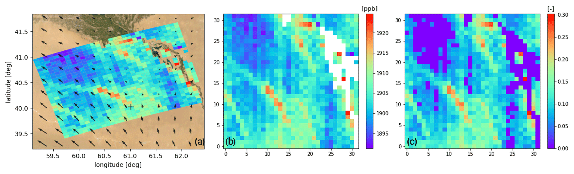
Figure 2 Atmospheric methane mixing ratios of a 32×32 pixel scene containing a methane plume originating from a known persistent source (indicated by the plus sign, +) as observed by TROPOMI on 5 December 2021 at 08:47 UTC (not included in the training data). (a) Mercator projection of the scene over Esri World Imagery (Esri, Maxar, Earthstar Geographics, and the GIS User Community, 2022), and arrows show the local GEOS FP 10 m wind field (Molod et al., 2012). (b) A 32×32 pixel scene in the along-orbit versus across-orbit direction indicating filtered pixels. (c) The same scene after pre-processing, as used by the CNN.

Figure 1 illustrates the full machine learning pipeline and training process. Section 2.1 describes the pre-processing step to generate scenes used by the CNN and the feature engineering algorithms. Section 2.2 describes the training process of the CNN (Fig. 1, CNN training). Section 2.3 describes the feature engineering algorithms, which are used to generate feature vectors for each TROPOMI scene. The SVC uses those feature vectors during its training process (Fig. 1, SVC training), covered in Sect. 2.4. Then, we apply the full, trained, machine learning pipeline to 2021 TROPOMI observations that the models have not been trained on (Fig. 1, CNN + SVC application). Based on the resulting TROPOMI detections, we perform further analysis (Sect. 2.5) and use (targeted) high-resolution methane observations (Sect. 2.6) to pinpoint the responsible sources for 12 of those detections.

2.1 TROPOMI

We use data over land from the TROPOMI $X_{{\mathrm{CH}}_{\mathrm{4}}}$ Level 2 scientific data product version 18_17. This product version is consistent with operational version 02.03.01 (Lorente et al., 2021; Hasekamp et al., 2022) but re-processed for the full time span of the mission resulting in a homogeneous data product (SRON CH4 L2 team, 2022). We use albedo–bias-corrected data with a quality assurance value (QA)≥0.4, methane precision < 10 ppb, SWIR aerosol optical depth < 0.13, near-infrared (NIR) aerosol optical depth < 0.30, SWIR surface albedo > 0.02, mixed albedo (2.4 ⋅ NIR surface albedo − 1.13 ⋅ SWIR surface albedo) < 0.95, and SWIR cloud fraction < 0.02. The loosened filtering compared to the recommended QA=1 filter provides more coverage but also retains more biased retrievals, especially at the borders of clouds or along coasts. The methane data are destriped, following the approach introduced by Borsdorff et al. (2018).

To train a machine learning model to recognize methane plumes in TROPOMI data, we created a dataset of scenes consisting of 32×32 pixels, both with and without methane plumes. The 32×32 pixels correspond roughly to an area of $\sim \mathrm{176}\times \mathrm{232}$ km² at nadir and up to $\sim \mathrm{176}\times \mathrm{448}$ km² for larger viewing angles. For scenes with plumes, we use data over 60 persistently emitting locations identified using long-term wind-rotated averages (Maasakkers et al., 2022b). By manual inspection, we compile a dataset of 828 positive scenes from 2018–2020 with plumes, of which 195 originate from coal mines, 203 from landfills/urban areas, and 430 from oil and gas infrastructure (Fig. 1, CNN training). An example scene is shown in Fig. 2a, including the local wind field at the time of observation.

A set of (negative) scenes without an emission signal was obtained through a manual inspection of six full orbits in different sections of the orbital repeat cycle, covering a diverse set of surfaces and (meteorological) conditions. We obtain 32×32 pixel scenes using a moving window algorithm with 50 % overlap, resulting in a dataset of 2242 scenes without a plume signal. The moving window algorithm later ensures that if a plume is cut in half in a particular scene, then it will be at the center of the adjacent – and partially overlapping – scene. Scenes with <20 % valid $X_{{\mathrm{CH}}_{\mathrm{4}}}$ pixels are discarded. This processing is applied to full orbits; the scenes with plumes originating from known locations were processed to match the same format. When combined, the dataset contains 3070 scenes used for training. The difference in the number of positive (828) and negative (2242) scenes is corrected for later on, using class weights. For each scene, we store 46 other channels of supporting information from the same TROPOMI Level 2 methane data product, including co-retrieved atmospheric properties, meteorological parameters, and geometric properties. These channels are used in later steps of the machine learning pipeline.

In order to correct for differences in local background concentrations (e.g., due to difference in latitude or surface altitude), each scene is normalized from 0 to 1. Values below the mean methane concentration of the scene minus 1 standard deviation are set to 0. Values above the mean plus 100 ppb minus 1 standard deviation are set to 1, and values in between are linearly distributed. Filtered pixels are set to 0. This pre-processing preserves the information of plume-like enhancements above the local background. Examples of the normalization input and output are shown, respectively, in Fig. 2b and c.

2.2 Convolutional neural network (CNN)

We use a convolutional neural network (LeCun et al., 2010) to detect methane plumes in the TROPOMI methane data that have been split into 32×32 pixel scenes. Convolutional neural networks (CNNs) are a type of machine learning model commonly applied in image recognition and object detection problems (Cheng et al., 2020). A CNN consists of multiple layers, where information moves from an input image, through the layers of the CNN at an increasingly abstract coarse resolution to the output, which is the classification of the image. To condense the information of the image to coarser resolution, the CNN uses “convolutional blocks” that consist of two or more convolutional layers, followed by a (max-) pooling layer. A convolutional layer produces “feature maps” that indicate where certain features (e.g., curves, edges, or more abstract features) are detected within the image. These feature maps are obtained by convoluting the input image with a convolutional kernel, which is a small matrix with weights that are optimized during training to best detect the features relevant to the particular classification problem. The resulting feature maps (one for each kernel applied) are then the input for the next layer (LeCun et al., 2010; Cheng et al., 2020). A max-pooling layer scans the previous layer with a 2×2 kernel and returns the maximum value, thereby creating a feature map at half the resolution that is focused on dominant features (LeCun et al., 2010). After the last convolutional block, the resulting feature maps are flattened and interpreted by one or more fully connected (dense) layers, consisting of neurons, between which the connections have trainable weights. This part of the network aggregates the information into a single output value. During training, the trainable weights, in the convolutional kernels and dense layers, are optimized to best perform the classification task, based on the training dataset (LeCun et al., 2010; Cheng et al., 2020). The trained CNN can then be used to classify new images, which are in this case labeled as “plume” versus “no-plume” images.

The main advantages of the CNN compared to regular neural networks or other machine learning models are that (1) the CNN is capable of better retaining spatial information which is lost in fully connected networks or machine learning models like decision trees or support vector machines (Selvaraju et al., 2020); (2) the training of a CNN can be done with image-level labels (plume or no plume), and there is no need to indicate where the feature of interest is located within the image, as the CNN learns to localize these features during training; (3) the same convolutional kernels are convoluted with the entire image, which is more computationally efficient compared to fully connected networks (LeCun et al., 2010; Cheng et al., 2020); and (4) the model is rotationally and translationally invariant when properly trained (LeCun et al., 2010).

This last model property is essential for the automated detection of plumes, as a plume can be located anywhere within a scene, and the wind can be in any direction. The CNN's output is a prediction between 0 and 1, indicating the confidence of the model about the presence of a plume-like structure. Scenes with prediction scores > 0.5 are classified as plumes. Although we use this output for binary classification, the value holds additional information regarding the confidence of the CNN (i.e., 0.6 versus 0.98), which we use for the second model.

We first select a high-level architecture for the CNN with standard hyperparameters, which we later optimize. Hyperparameters are model settings, separate from the trainable weights, such as the number of convolutional layers and kernel sizes and also parameters that influence the training process, such as the learning rate. As high-level architecture we selected two convolutional blocks followed by two fully connected layers and an output neuron (Fig. 3). We found that deeper networks (e.g., ResNet, He et al., 2016, or VGG-16, Simonyan and Zisserman, 2014) did not yield an improvement in performance for this problem with relatively low-resolution, small-sized (32×32 pixel) scenes.

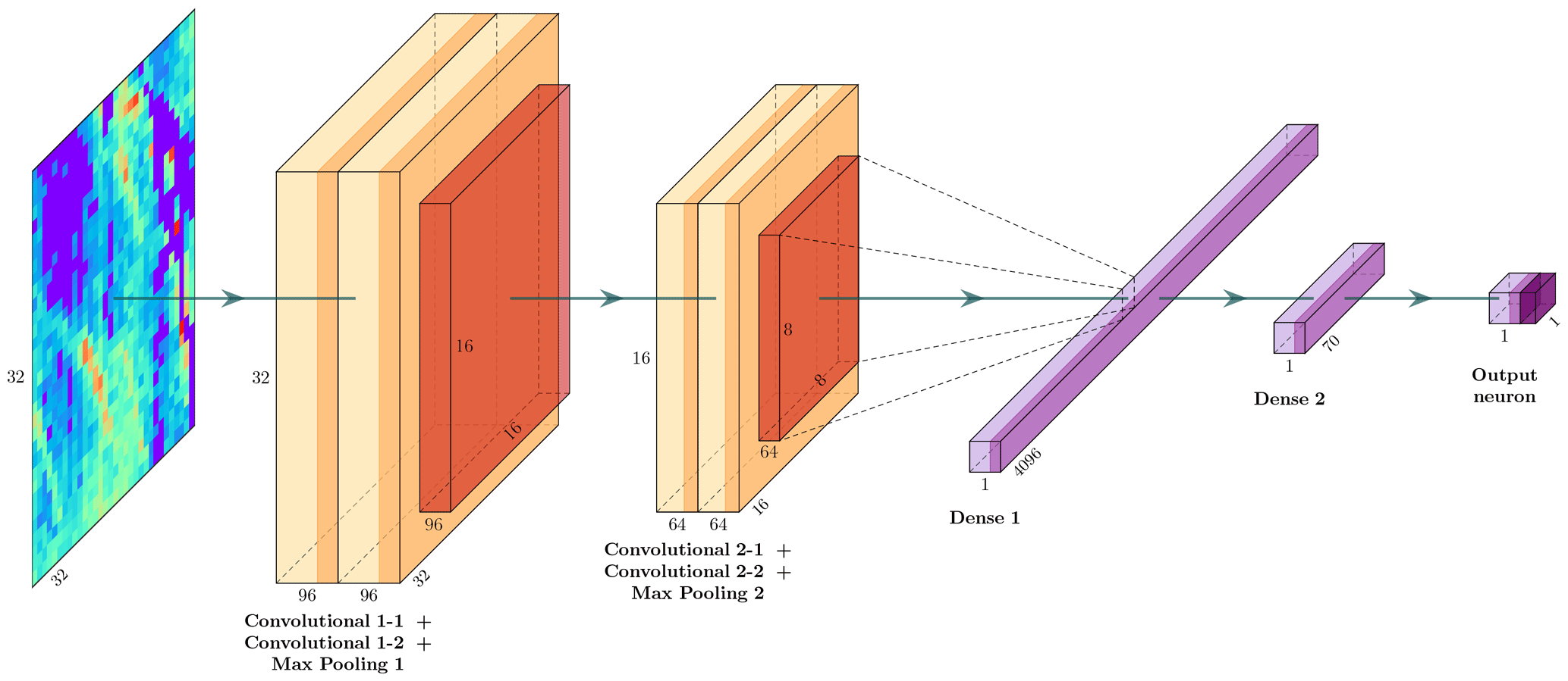
Figure 3 A schematic overview of the convolutional neural network with a pre-processed 32×32 pixel TROPOMI methane scene (Fig. 2c) as input (left). The CNN consists of two convolutional blocks (each with two convolutional layers followed by a max-pooling layer), followed by two dense (or fully connected) layers and an output neuron with sigmoid activation. Numerical values show the input dimensions, layer dimensions, and the number of feature maps in the convolutional and max-pooling layers. Visualization generated using PlotNeuralNet (Iqbal, 2018).

Our training dataset mostly contains clear positives (828) and clear negatives (2242) to effectively learn the distinguishing features. Our dataset has many more negative than positive scenes. When training our CNN, however, we want both categories of training samples (classes) to have equal impact in order to obtain optimal performance (Johnson and Khoshgoftaar, 2019). This balancing can be achieved by applying class weights during training (Johnson and Khoshgoftaar, 2019), giving positive scenes more weight. We set the class weight parameter to the inverse of the ratio between the number of positives and negatives. We randomly split the data into a training (80 %) and test (20 %) set. Then, 20 % of the training scenes are used as validation subset (Table A1). The validation dataset is used to infer whether there is a generalized performance increase during the training of the CNN to prevent overfitting. We then augment the data in order to obtain larger training and test sets; all scenes are rotated 90^∘ thrice and flipped, thus enlarging the datasets by a factor 8.

We use the training dataset of 19 648 (augmented) scenes (Table A1) to train the CNN (Fig. 1, CNN training). The CNN was designed and trained using the machine learning framework Keras (Chollet et al., 2015; Chollet, 2021) by first using the default values for the hyperparameters. The model is trained for a maximum of 100 epochs (iterations of the training process). During training, we optimize the validation loss, which measures the error made on the subset of the training data not used in that epoch. We use binary cross-entropy as the loss function and Adam (an improved version of stochastic gradient descend algorithm; Kingma and Ba, 2014) as the optimizer. We use a 0.4 dropout layer (randomly disabling 40 % of the neurons) in the first fully connected layer during training to prevent overfitting and make the model more robust (Srivastava et al., 2014). The activation function modifies the output before it is passed to the next layer; we apply the ReLU (rectified linear unit, which outputs zero when the input is negative and otherwise outputs the input value) activation function in all layers, except for the final layer where we apply sigmoid ($\frac{\mathrm{1}}{\mathrm{1}+e^{-x}}$), which normalizes the output. To force the model to focus more on plume-like signatures during training, the loss weight of plume scenes is set to double that of the negatives scenes. Training is halted after the validation loss does not improve for several epochs, and the best model weights found up to that point are used. After training, the model performance is inferred by classifying the labeled test dataset.

After training this initial “default” model version, the hyperparameters were further optimized using the KerasTuner optimization framework (O'Malley et al., 2019) and Hyperband (Li et al., 2018). With these methods, we perform a grid search to find the best hyperparameters for our particular problem. The optimal hyperparameters depend on the size of the training dataset, architecture of the CNN, number of classes, and problem type. The search space for the optimization was defined using insights from the initial training, theoretical foundation, and design constraints. We inspected the hyperparameters of the top 10 performing setups and selected the optimal hyperparameters by combining the results of this optimization with expert judgment on this particular problem. Figure 3 shows a schematic overview of the CNN with optimized hyperparameters.

We evaluate the performance of the CNN using performance evaluation metrics (Eq. 1) calculated from the number of true positives and negatives (TPs and TNs), and false positives and negatives (FPs and FNs; Johnson and Khoshgoftaar, 2019). Cohen's κ score (Cohen, 1960) is a weighted accuracy which takes into account the class imbalances and chance agreement. The recall indicates which fraction of plumes present in the test set is correctly identified, and the precision indicates which fraction of scenes identified as plumes is actually a plume; the F1 score incorporates both into a single metric.

$$\begin{array}{}\text{(1)}& \begin{array}{rl}& \mathrm{Accuracy}={\displaystyle \frac{\mathrm{TP}+\mathrm{TN}}{\mathrm{TP}+\mathrm{TN}+\mathrm{FP}+\mathrm{FN}}}\\ & \mathrm{Precision}={\displaystyle \frac{\mathrm{TP}}{\mathrm{TP}+\mathrm{FP}}}\\ & \mathrm{Recall}={\displaystyle \frac{\mathrm{TP}}{\mathrm{TP}+\mathrm{FN}}}\\ & \mathrm{F}\mathrm{1}=\mathrm{2}\cdot {\displaystyle \frac{\mathrm{precision}\times \mathrm{recall}}{\mathrm{precision}+\mathrm{recall}}}\end{array}\end{array}$$

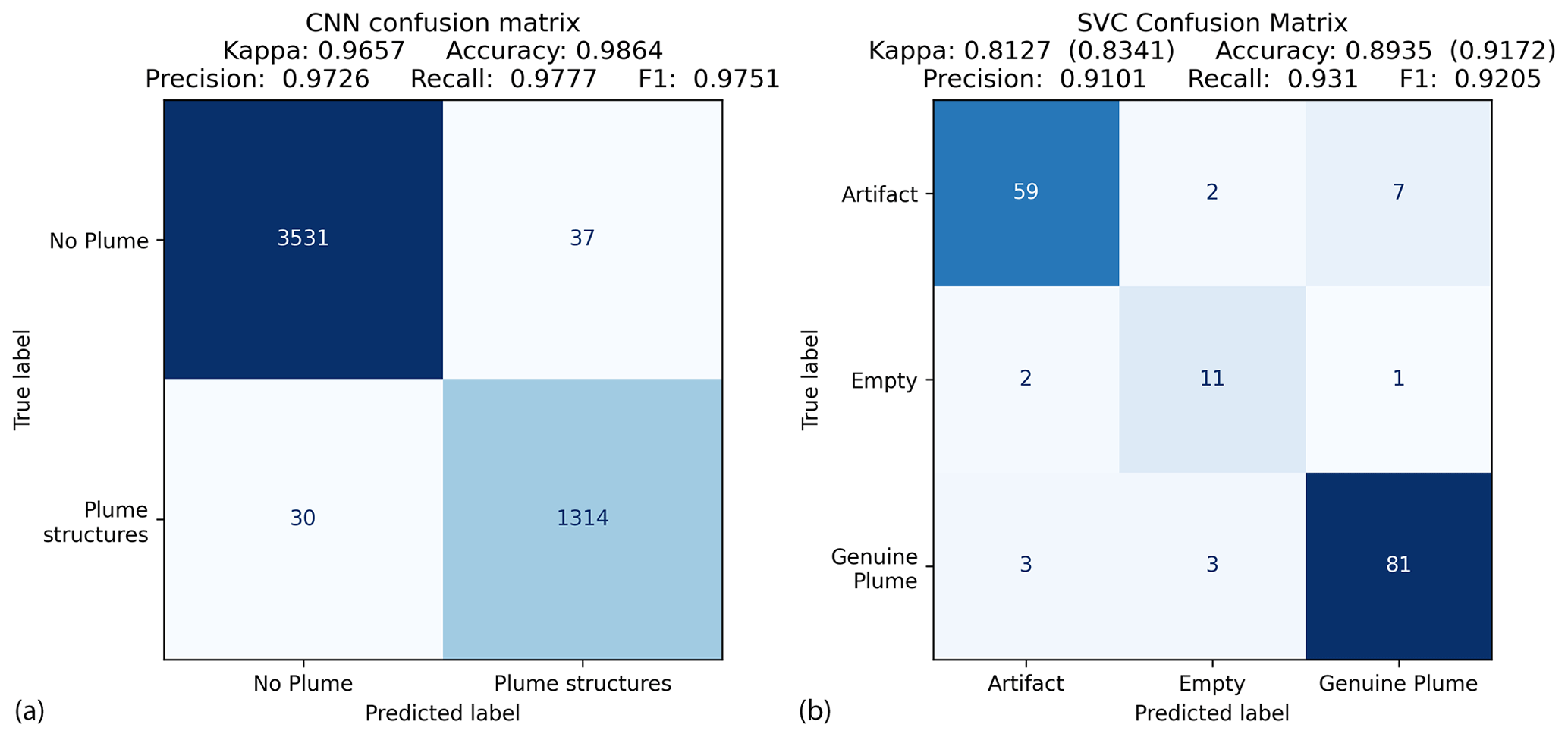
Figure 4 Confusion matrices showing the performance of the CNN (a) and the SVC (b) on their corresponding test datasets. The performance metrics are defined in Eq. (1), and the values in parentheses for the SVC show the performance when the problem is considered to be a binary problem; i.e., when “Artifact” and “Empty” are combined as “No Plume”.

To test the influence of the split of the training and test datasets (which can be an issue for datasets of a limited size), the training of the model with optimized hyperparameters was repeated 50 times with different splits. We found that model performance is relatively insensitive to different training splits, with $\mathit{\kappa }=\mathrm{0.943}\pm \mathrm{0.012}$, recall = 0.956±0.014, and F1 = 0.958±0.009 (standard deviations). We further found that small changes in the hyperparameters have an even lower effect when compared to different training splits. The consistent performance on the corresponding test datasets shows that the model is robust and well generalized. We focus on recall over precision because the key focus is to have as few potential plumes as possible go undetected. We selected the model which scored best on κ, second best on F1 score, and third best on recall. The performance metrics of the selected CNN are shown in Fig. 4a. Manual inspection of the misclassified scenes (30 FNs and 37 FPs out of 4912 augmented test scenes) indicates that these are borderline cases with difficult-to-discern morphological structures that are even challenging to a human expert.

The trained CNN is applied to all 2020 data. Processing of the 5193 orbits of 2020 resulted in 752 890 scenes (only taking into account scenes with >20 % valid pixels), of which 25 626 scenes (3.4 %) are identified as containing plume-like morphological structures by the CNN. This number does include artifacts and duplicates, due to the moving window algorithm, as these are filtered later on. We use a subset of these scenes to train the second step of the machine learning pipeline (Sect. 2.4).

2.3 Feature engineering

Due to the difficult nature of methane retrievals, not every plume-like morphological structure in the $X_{{\mathrm{CH}}_{\mathrm{4}}}$ field is an actual methane plume. Different types of surface variability and atmospheric or meteorological conditions are known to affect the retrieval (Lorente et al., 2021); if there is a strong correlation between the methane enhancement and retrieval parameters, e.g., the surface albedo or the aerosol scattering coefficient, then the retrieved methane enhancement might be caused by the albedo or aerosol variation and could therefore be a retrieval artifact. Other common examples of artifacts are those on the borders of clouds and coastlines or when the direction of the enhanced structure is not in agreement with the wind field but with surface structures instead.

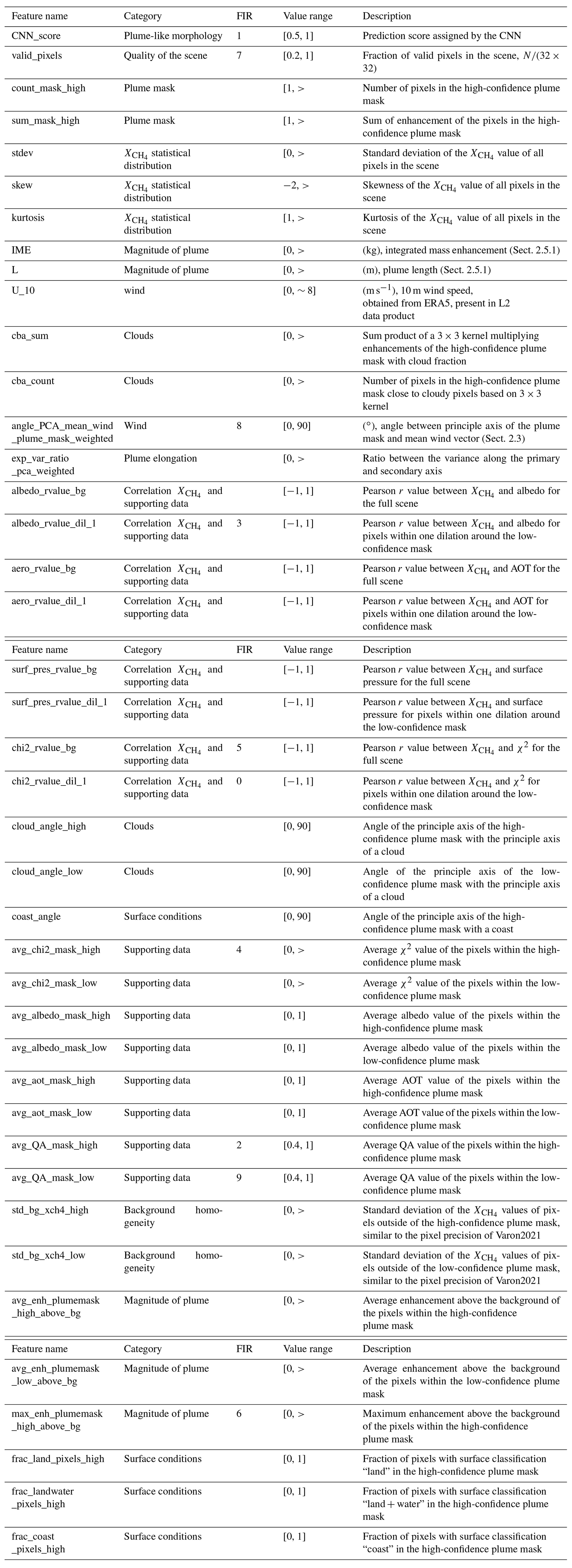
In order to automate the necessary further inspection, we compute numerical values for several features of potential plumes through feature engineering. Feature engineering is a commonly applied approach in machine learning problems and is especially helpful when limited amounts of labeled training data are available. These features are a representation of the information that a human expert would use to inspect the potential plumes in order to determine whether a scene contains a genuine plume or an artifact. We construct feature vectors consisting of features based on the corresponding scene. These vectors are then used to train the second model of the machine learning pipeline, which is the SVC (Fig. 1, SVC training). An overview of all the developed features is presented in Table C1.

Fundamental to many of those features is masking the plume in order to isolate the plume pixels from the background. For this purpose, we use information about which part of the scene has triggered the CNN detection. For this, we use the class activation map (CAM) to visualize the localized activations of a CNN corresponding to a certain class on which it was trained (Zhou et al., 2015). We apply Grad-CAM (Selvaraju et al., 2020), which allows the computation of the CAM for our CNN that includes fully connected layers. In our binary classification problem, the CAM visualizes which regions of the deepest (coarsest) feature maps (max pooling 2 (8×8) in Fig. 3) contribute strongest to an activation of the plume class (output > 0.5) for a given input image. This spatial activation is calculated using the gradients (Selvaraju et al., 2020) between the 64 feature maps (each of 8×8 resolution, resulting in a $\mathrm{64}\times \mathrm{8}\times \mathrm{8}$ array; Fig. 3) of the deepest max-pooling layer (max pooling 2) and the first fully connected or dense layer (dense 1 in Fig. 3). In order to obtain a CAM with a sufficient resolution, we limit the depth of the CNN to two convolutional blocks. The CAM is upsampled to match the input resolution (Selvaraju et al., 2020). Figure 5b shows that the CAM correctly identified the plume-like structure in the $X_{{\mathrm{CH}}_{\mathrm{4}}}$ scene in Fig. 5a, thus disregarding the noisy high-enhancement pixels elsewhere in the scene.

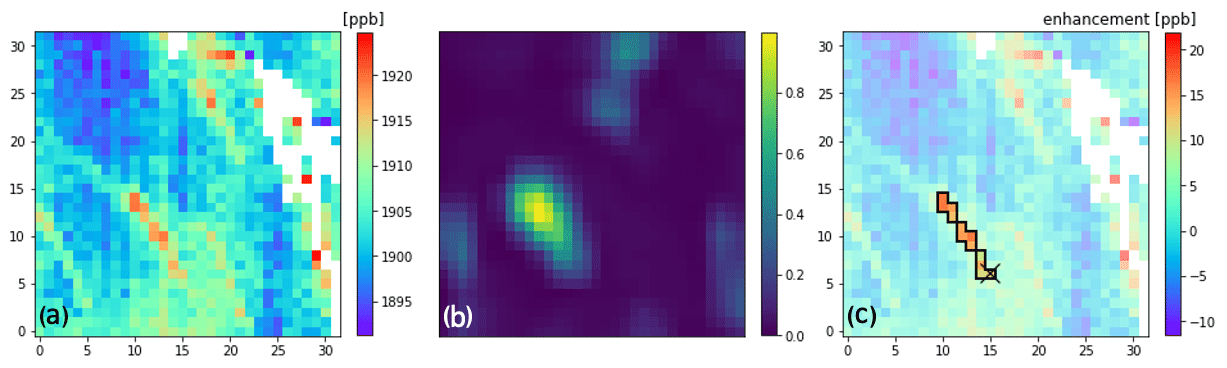
Figure 5 Several feature engineering results computed for the 32×32 scene from Fig. 2. (a) The atmospheric dry-air methane column mixing ratios $X_{{\mathrm{CH}}_{\mathrm{4}}}$. (b) The class activation map, which highlights the areas identified by the CNN as being plume-like structures, based on Fig. 2c, the pre-processed scene, and (c) the methane enhancements relative to the local background, with the black line indicating the high-confidence plume mask. The pixel with the cross (×) is identified as being the pixel most likely to contain the source location, based on the plume mask and local wind field (shown in Fig. 2a).

In addition to using the CAM to analyze CNN performance, we also use it to generate a binary plume mask. We multiply the CAM with the enhancement above the mean $X_{{\mathrm{CH}}_{\mathrm{4}}}$ value minus the scene's standard deviation. The output is a map highlighting pixels with high methane enhancements that are identified as part of the plume by the CNN; we identify the pixel with the maximum value as the starting point for the plume mask. To compute a “high-confidence” plume mask, we start from the corresponding pixel in the $X_{{\mathrm{CH}}_{\mathrm{4}}}$ image and dilate outwards (including diagonally). We only add adjacent pixels with enhancements of 1.8 standard deviations above the mean (Fig. 5c). We repeat this process with a lower threshold of 0.8 standard deviations to also obtain a “low-confidence” mask; both thresholds were established empirically. This approach ensures that noise in other parts of the image is excluded from the plume mask. A plume mask can consist of any number of pixels, depending on the scene. The minimum is 1 pixel, but this is rare, as the average is around 20 pixels. Several statistics of the (potential) plume can be computed using these masks with supporting data.

One of the major indicators of an artifact is a strong correlation with one or more retrieval parameters. If an enhancement in the $X_{{\mathrm{CH}}_{\mathrm{4}}}$ field is caused by a surface (albedo) feature or by (enhanced) scattering in the atmosphere which is represented by the aerosol optical thickness, then we expect their spatial patterns to be similar. Therefore, we calculate the correlation between $X_{{\mathrm{CH}}_{\mathrm{4}}}$ and the surface albedo (SWIR), aerosol optical thickness, χ² (an indicator for retrieval fit quality), and surface pressure across the plume mask. We calculate these correlations for the high- and low-confidence plume masks, 1- and 2-times dilated versions of the low-confidence mask, and the entire scene. We account for pixels outside of the plume mask, as we would expect a strong correlation around the enhancement if it is an artifact. The correlations over the entire scene reflect large-scale patterns that do not necessarily imply artifacts.

Another major indicator for artifacts is a mismatch between the direction of the plume and the direction of the local 10 m wind field from the ERA5 reanalysis (Hersbach et al., 2020) included in the TROPOMI Level 2 data product (Hasekamp et al., 2022). By applying a principle component analysis (PCA), we compute the two main axes of the pixels in the high-confidence plume mask, after re-projecting the pixel centers to meter space and weighting them by their enhancement relative to the background. We use the ratio of the variances described by the axes as a measure of the plume's elongation. For elongated plumes (e.g., Fig. 5), the variance of the primary axis is much larger than the variance projected to the secondary axis, while for less elongated, blob-like plumes, this ratio is small. Furthermore, we compare the angle of the primary axis of the potential plume to the angle of the wind direction (averaged across the plume mask); the smaller the difference, the more confidence we have in the plume following the wind. We also use the wind field to identify the pixel that most likely contains the plume's source by taking the most upwind pixel within the high-confidence plume mask (Fig. 5c).

2.4 Support vector classifier (SVC)

A support vector classifier (SVC) constructs hyperplanes as the optimal decision boundary to separate multiple classes in a high-dimensional feature space. SVCs in general perform better with datasets of limited size compared to deep learning algorithms and are in general less prone to erroneous influence from outliers. We use 843 labeled scenes from 2020 classified by the CNN to contain plume-like structures as a training dataset for the SVC (Fig. 1, SVC training). About half of the scenes are randomly selected from within seven geographical zones with specific types of predominant artifacts, and the other half is selected randomly. Scenes are labeled as “plume” (444 scenes), “artifact” (341 scenes), or “empty” (58 scenes, indicating there is not a clear plume or artifact). We have only included scenes with unambiguous labels. The fact that there are relatively few empty scenes in this subset indicates that the CNN performs well. We use balanced class weights to correct the imbalance in the number of training samples per class, and the weights are inversely proportional to the number of scenes in each class.

The data format we use for the SVC is a vector of 41 features, and each feature vector corresponds to a 32×32 pixel scene. This feature vector includes correlations with retrieval parameters for different plume masks, the angle between the wind and elongated direction of the plume, the elongation ratio of the plume, several intermediate outputs of the source rate estimate (Sect. 2.5.1), and several statistical properties (all engineered features are listed in Table C1). We do not include features such as latitude and longitude or distance to a known source or known infrastructure in order to be unbiased with respect to where a scene is located. We train the SVC to find the optimal classification boundary within this 41 dimensional space, based on the 843 labeled feature vectors. Each feature is standardized by subtracting the mean and scaling the value to the unit variance of that feature in the entire training set. We use a radial basis function (RBF) kernel and set the regularization parameter to 1.2; this hyperparameter was optimized using a simple grid search optimization. The gamma value is scaled inversely to the number of features (41 in this case) multiplied with the variance of the training dataset, as is common practice, and helps to homogenize the features which have different units and ranges of values (Table C1).

We randomly split the labeled dataset into a training set (80 %) and a test set (20 %). Contrary to the CNN, when training an SVC, no validation set is used. Correctly detecting plumes is of predominant interest; therefore, we combine non-plume scenes (artifact and empty classes) when evaluating the performance. We train the model 2000 times for different splits of the dataset. The distribution of these different realizations shows convergence with binary $\mathit{\kappa }=\mathrm{0.78}\pm \mathrm{0.04}$ and recall = 0.88±0.03 (standard deviations), indicating that the model setup is not too dependent on the data split. We select a model with relatively high κ and recall, where performance is similar between the training and test sets. Figure 4b shows the three class performances on the test set, indicating that distinguishing between plumes and artifacts is the most challenging distinction for the SVC. The binary Cohen's κ score of the selected model is 0.83. A κ score of above 0.8 is generally seen as being a good classification performance. The recall is 0.93, meaning that 93 % of the scenes with plumes which were present in the test set are successfully identified, and only 7 % of the plumes are missed.

To evaluate which features are important for the SVC to classify a scene, we performed a permutation importance analysis perturbing each feature 40 times (Breiman, 2001). Based on the resulting mean feature importance, the most important features are the correlation of $X_{{\mathrm{CH}}_{\mathrm{4}}}$ with χ², the CNN score, the albedo correlation, the enhancement of the plume, the fraction of valid pixels, the angle with the local wind, and the average quality flag of plume pixels (the top 10 ranking of feature importance metrics is presented in Table C1). These correspond to what is important to a human expert labeler.

2.5 Plume characterization

2.5.1 Source rate quantification

To estimate the source rates of the plumes observed by TROPOMI, we apply the integrated mass enhancement (IME) method (Frankenberg et al., 2016; Varon et al., 2018). Some intermediate outputs of the IME method (such as the plume length) are used as features in the feature vector for the SVC (Sect. 2.4). We perform a full source rate quantification, including uncertainty estimates, for the plumes that pass the machine learning pipeline and are manually verified. The IME method relates the emission rate (Q) to the observed methane enhancement in the plume (IME) and the local wind field as follows (Varon et al., 2018):

$$\begin{array}{}\text{(2)}& \begin{array}{rl}& Q={\displaystyle \frac{\mathrm{1}}{\mathit{\tau }}}\mathrm{IME}={\displaystyle \frac{U_{\mathrm{eff}}}{L}}\mathrm{IME}\\ & \mathrm{IME}=\sum _{j=\mathrm{1}}^N\mathrm{\Delta }{\mathrm{\Omega }}_j{A}_j,\end{array}\end{array}$$

where ΔΩ_j denotes the methane column mass enhancement above the local background of pixel j, with the footprint A_j. The local background is calculated as the median value of the scene's pixels outside the high-confidence plume mask. The IME of all N pixels in the plume is related to the source rate, using the average residence time τ of methane particles in the plume, with τ being given by the ratio between the plume length L and the effective wind speed U_eff. The plume length L is approximated as $L=\sqrt{A_{\mathrm{M}}}$, where A_M is the area of the plume mask (Varon et al., 2018). U_eff can be expressed as a function of the local (reanalysis) wind speed. Frankenberg et al. (2016) and Varon et al. (2018) developed the IME method for high-resolution instruments, for which the 10 m winds are most representative of U_eff values. For the larger scale of TROPOMI plumes, both 10 m (U₁₀) and boundary layer average (U_PBL) winds have been used (Varon et al., 2019; Schneising et al., 2020; Cusworth et al., 2021; Tu et al., 2022a). As the most representative wind can vary from case to case, we use the mean of the quantifications using ERA5 10 m winds (Hersbach et al., 2020), GEOS FP 10 m winds, and GEOS FP planetary boundary layer (PBL) winds (Molod et al., 2012).

We calibrate the relation between U_eff and these local wind speeds by quantifying 15 336 plumes simulated with the Weather Research and Forecasting model coupled with a Chemistry module (WRF-Chem), version 4.1.5 (Skamarock et al., 2019; Grell et al., 2005). The model uses 38 vertical levels and three nested domains at a horizontal resolution of up to 4×4 km². Physical parameterizations and meteorological initial and boundary conditions are as described in Dekker et al. (2017). We release passive tracers with emission rates mostly between 10–100 t h⁻¹ at various locations in western Asia, Mexico, and Argentina for June–September 2019 and 2020. We sample the plume at the TROPOMI overpass time and quantify them as described above.

Using the model wind speeds and known emission rates, we find that U_eff's dependence on the PBL wind is best described by a linear relationship, where $U_{\mathrm{eff}}={\mathit{\alpha }}_{\mathrm{1}}\cdot U_{\mathrm{PBL}}+{\mathit{\alpha }}_{\mathrm{2}}$, with α₁=0.47 and α₂=0.31 (r²=0.78). For the dependence on U₁₀, we also find a linear relation to be optimal and constrain α₂ to be non-negative, where $U_{\mathrm{eff}}={\mathit{\alpha }}_{\mathrm{1}}\cdot U_{\mathrm{10}}+{\mathit{\alpha }}_{\mathrm{2}}$, with α₁=0.59 and α₂=0.00 (r²=0.77). We use the mean of the three resulting U_eff values to quantify emissions.

To estimate the uncertainty, we create an ensemble of estimates by varying the parameters influencing the quantification. For each of the different input wind speeds, we vary the threshold for masking the plume from 1.3 to 2.3 standard deviations (step 0.1), adjust the background concentration by ±2 times the mean $X_{{\mathrm{CH}}_{\mathrm{4}}}$ uncertainty in the scene (step 0.4), vary the wind values from −50 % to +50 % (step 10 %), and vary α₁ and α₂ for −5 % to 5 % (step 1 %). We report the standard deviation of the resulting 43 923 member ensembles as being the uncertainty for each plume.

2.5.2 Removal of duplicate scenes

Due to the moving window algorithm, each group of 16×16 pixels is seen by the machine learning pipeline up to four times as a different corner of a 50 % overlapping 32×32 pixel scene. This ensures that the plumes do not go undetected because they are cut in half and allows multiple nearby plumes to be detected in adjacent scenes but also leads to duplicate detections. Therefore, plumes for which the generated plume mask overlaps with a plume mask from another scene are grouped into a group. For each group, the scene with the highest IME value is selected.

2.5.3 Anthropogenic source sector estimation

To assess which anthropogenic activity might underlie a detected plume, we use the estimated source location to find the local dominant source type in gridded bottom-up inventories. We exclude sectors that are unlikely to produce point source emission signals in single overpass TROPOMI data, such as rice cultivation and livestock. We include 2019 oil, gas, and coal emissions from the updated Global Fuel Exploitation Inventory (GFEI v2; Scarpelli et al., 2022a) and 2018 landfill emissions from EDGAR V6.0 (Crippa et al., 2021). We identify the dominant source type as being the source type with the largest annual flux in a $\mathrm{0.7}{}^{\circ }\times \mathrm{0.7}{}^{\circ }$ square centered around the estimated source location. Based on known emitters, we found that using a window of this size mitigates errors in the estimated source location and spatial errors in the emission inventories. We do not use this approach to attribute detections to wetlands. However, we do inspect 2019 fluxes from the WetCHARTs v1.3.1 ensemble (Bloom et al., 2021) to identify regions where detections might be influenced by strong wetland fluxes, such as in central Africa (Pandey et al., 2021).

2.5.4 Comparison with a previously studied super-emitter event

In order to test the automated pipeline and feature engineering algorithms, we apply it to data over a September 2019 super-emitter event in Louisiana, USA (Maasakkers et al., 2022a). The model detects the emission event on multiple days, including on the first day with large emissions and significant TROPOMI coverage (25 September). The CNN score is >0.999, and the SVC classified the scene as a plume. The estimated source location of the plume is 2.2 km away from the source, and our automated quantification estimate is 121±46 t h⁻¹. Our estimate is in good agreement with the quantification by Maasakkers et al. (2022a) of 101 (49–127) t h⁻¹, which scales a plume simulated with the WRF atmospheric transport model to match the enhancements seen in TROPOMI using a Bayesian inversion.

2.6 High-spatial-resolution methane satellite instruments, retrievals, and source rate quantification

We use observations from three high-spatial-resolution instruments, GHGSat, PRISMA, and Sentinel-2, to inspect the sources of the detected methane plumes. This section describes the main characteristics of these instruments.

2.6.1 GHGSat

GHGSat-Cx instruments are Fabry–Pérot imaging spectrometers that were launched in 2020–2022 (C1–C5), building on the GHGSat-D instrument (Jervis et al., 2021). The instruments have a spatial resolution of 25 m × 25 m over targeted scenes of ∼10 km × ∼15 km (Ramier et al., 2020; MacLean et al., 2021). They sample the SWIR part of the spectrum between 1630 and 1675 nm at ∼0.3 nm spectral resolution, retrieving the methane column density with a precision of 1 % of the background concentration and a theoretical detection threshold of down to ∼100 kg h⁻¹ at a wind speed of 3 m s⁻¹ (ESA, 2022). During a controlled release experiment comparing the methane observing capabilities of different high-resolution instruments by Sherwin et al. (2023), a plume of ∼200 kg h⁻¹ was successfully detected. We use data from GHGSat-C1 and GHGSat-C2 and estimate the source rates using the IME method, as described in Maasakkers et al. (2022b), for point sources with 10 m wind data from GEOS FP (Molod et al., 2012). The uncertainty in the quantification is estimated, as described by Varon et al. (2019), taking into account the error contributions from measurement noise, the wind speed, and the IME method, similar to Maasakkers et al. (2022b).

2.6.2 PRISMA

The Italian Space Agency's hyperspectral instrument PRISMA was launched in March 2019 and generates publicly available targeted hyperspectral 30 km × 30 km images at a spatial resolution of 30 m × 30 m and ∼10 nm spectral resolution (Cogliati et al., 2021; Guanter et al., 2021; Cusworth et al., 2021). The revisit time can be as short as 7 d, using the instrument's ±20 % across-track pointing (Cogliati et al., 2021). The smallest source rate tested during a controlled release experiment (Sherwin et al., 2023) is ∼2500 kg h⁻¹. The theoretical detection threshold is lower (∼300–900 kg h⁻¹ for homogeneous scenes) and strongly depends on the surface type/homogeneity (Guanter et al., 2021). The PRISMA instrument is not a continuous mapper, but a data archive of past (targeted) observations is publicly available. PRISMA can also be used to target a location of interest in the future. We perform methane retrievals and IME quantifications, as described in Guanter et al. (2021), using plume masking, following Varon et al. (2018), and GEOS FP 10 m wind data (Molod et al., 2012).

2.6.3 Sentinel-2

The Sentinel-2 surface-imaging mission (consisting of Sentinel-2A launched in 2015 and Sentinel-2B launched in 2017) was demonstrated by Varon et al. (2021) to be capable of detecting methane super-emitter plumes under favorable conditions. Both satellites carry a MSI, with a pixel resolution of 20 m × 20 m for the B11 (∼100 nm) and B12 (∼200 nm) SWIR bands, with a sensitivity to methane. The instruments have a 290 km wide swath, resulting in a global 2–5 d revisit time (Drusch et al., 2012). Sentinel-2 observes continuously (as opposed to GHGSat and PRISMA) and provides an extensive, publicly available archive going back years. A methane absorption signal has to be strong in order to stand out within the aggregated signal of the entire band; therefore, only relatively large quantities of methane can be retrieved, and the detection limit worsens considerably over non-homogeneous terrain. The detection limit is estimated at ∼1–2 t h⁻¹ for homogeneous scenes (Gorroño et al., 2023), which is in agreement with Sherwin et al. (2023), where a ∼1800 kg h⁻¹ emission was detected and quantified. We apply the methane retrieval and IME quantification approach from Gorroño et al. (2023), who, like Varon et al. (2021), use a reference day without a plume to isolate the difference caused by methane concentration enhancement. We again use GEOS FP 10 m wind data (Molod et al., 2012).

3 Results

We apply the trained and optimized CNN and SVC models (Fig. 1, CNN training and SVC training) in sequence on all 2021 TROPOMI $X_{{\mathrm{CH}}_{\mathrm{4}}}$ data (Fig. 1, CNN + SVC application). Analyzing the full year with the machine learning pipeline takes approximately 3 h on a single core. From the 794 395 (32×32 pixel) scenes, the CNN identifies 26 444 scenes (3.3 %) that contain plume-like $X_{{\mathrm{CH}}_{\mathrm{4}}}$ morphological structures. The SVC classifies 10 430 of these scenes as plumes. After duplicate removal, 4869 scenes are identified as unique. These 4869 scenes are manually inspected to assess the performance of the pipeline. We confirm 2974 scenes as being confident plumes. Another 745 scenes are labeled as potential plumes; accepting these scenes as plumes results in a precision of 76 % for the full pipeline. These potential plumes could not readily be verified as being real methane plumes but are valuable for further inspection. The remaining scenes are either labeled as artifacts or not containing a (concentrated) plume. These misclassifications can be used to further optimize the machine learning pipeline. Here, we will focus on the 2974 confident plumes and present the result of our high-resolution satellite instrument analysis to pinpoint the exact sources of 12 (clusters of) detections.

3.1 Overview of the confirmed detections in 2021

Figure 6 shows the spatial distribution of all 2974 detected and confirmed 2021 plumes, which are attributed by source sector, based on the three bottom-up inventories (Sect. 2.5.3). We find that 1031 plumes predominantly relate to urban areas and/or landfills, 720 to gas infrastructure, 612 to oil infrastructure, and 581 to coal mines. As super-emitters are usually not the result of regular operations and are therefore not well represented in bottom-up inventories, especially large transient emissions may be misattributed by this approach. Wetlands are not expected to result in point source emissions, but strongly emitting wetlands in central Africa, such as South Sudan and in the Niger delta, can produce large enhancements in the TROPOMI data (Pandey et al., 2021; Shaw et al., 2022). In the absence of large anthropogenic emissions, we label the plumes from these two regions as “unclassified”. Wetlands might also contribute to detected signals in areas with large anthropogenic emissions, for example, around the city of Dhaka, located in the Ganges–Brahmaputra Delta (Bangladesh), or in the Mississippi Delta (USA).

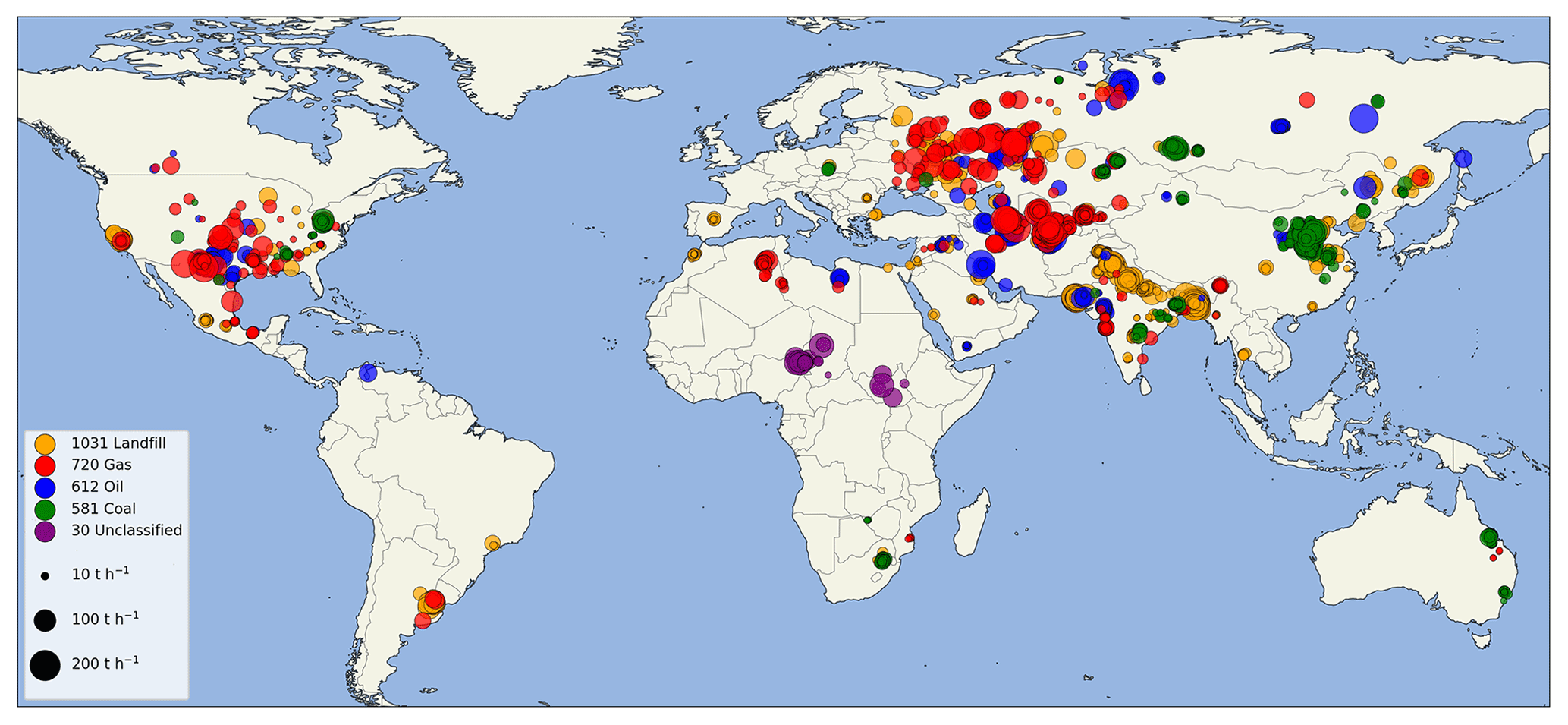
Figure 6 All 2974 confident plume detections for 2021, grouped into one of four dominant anthropogenic source types and sized by source rate, capped at 200 t h⁻¹. There are 30 detections in central Africa that are labeled as “unclassified”.

There are many clear hotspot locations with frequent detections. To group the detections into clusters with a common source, we apply the DBSCAN clustering algorithm (Ester et al., 1996; Schubert et al., 2017). We cluster based on the distance between detections in meters and set a threshold of five detections within 30 km as the minimum to identify a cluster. We identify 94 clusters; this is a conservative estimate for the number of persistent locations, as some known persistent emitters have fewer than five detections in 2021. We also observe several areas with extensive plumes from multiple emitters, such as the west coast of Turkmenistan, which are grouped into one big cluster. We find the majority of detected plumes (74.8 %) to be clustered at a persistent urban or fossil fuel exploitation source and classify the remaining plumes as transients. Zoom-ins of the clusters in several distinct regions and source rates for all detections are shown in Fig. 7.

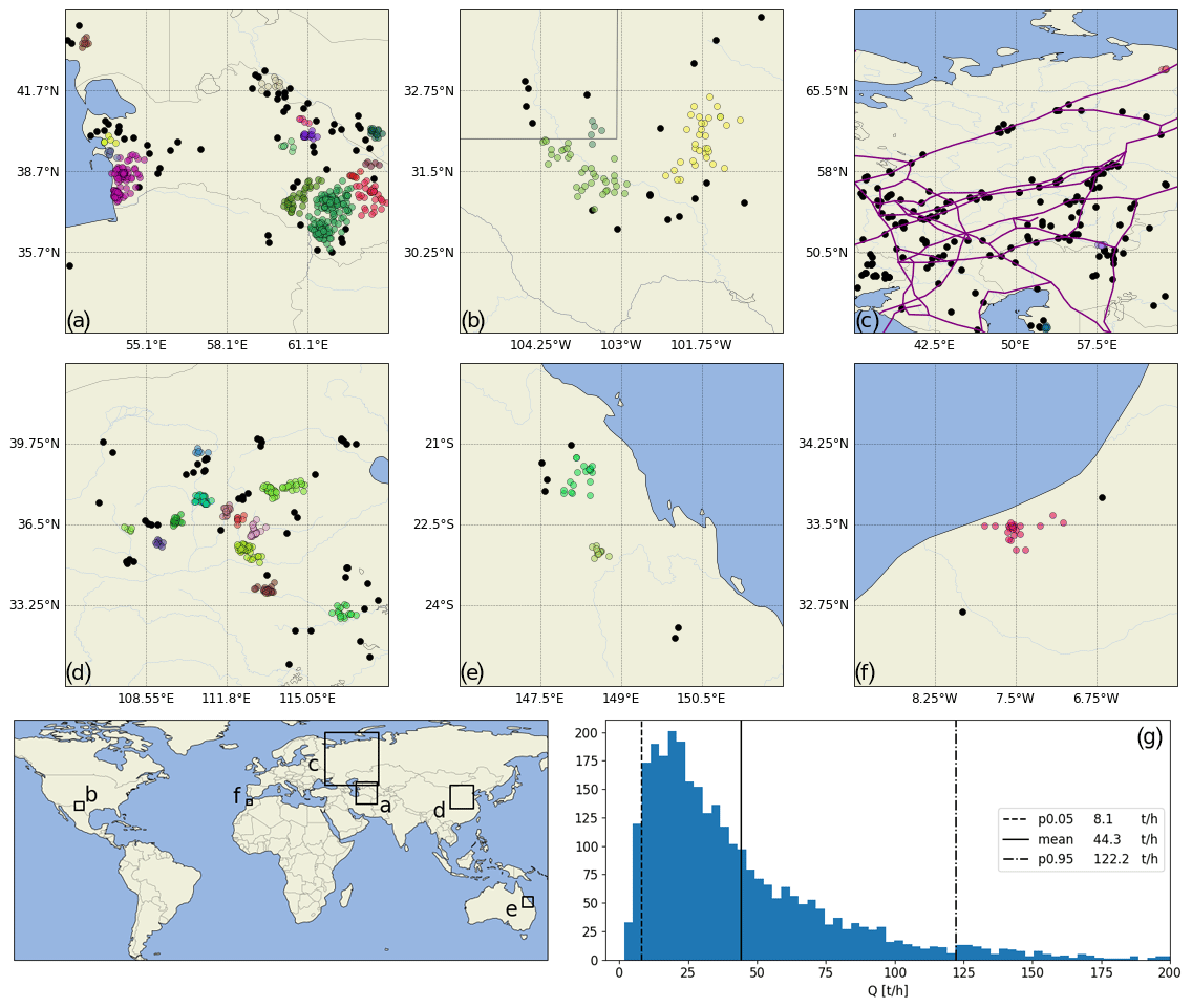
Figure 7 Regional plume detections showing color-coded persistent emission clusters, with transient emissions shown in black. (a) Large clusters of detections related to oil and gas exploitation in Turkmenistan. (b) The clearly distinguishable outlines of the Delaware and Midland sub-basins within the Permian Basin, USA. (c) Detections show the same spatial structure along compressor stations and pipelines in western Russia. (d) Clusters of hotspots in eastern China with the extensive Shanxi coal mining region in the center. (e) Clusters of coal mining detections in northeastern Australia. (f) A clear cluster of detections around the persistent source in Casablanca, Morocco. (g) The distribution of estimated source rates for all 2974 detected plumes in the year 2021, capped at 200 t h⁻¹. The 5th and 95th percentile and the mean values of the distribution are shown as vertical lines.

Several of the identified clusters are located over well-known oil and gas production regions, such as the west coast of Turkmenistan (Fig. 7a), previously studied by Varon et al. (2019) and Irakulis-Loitxate et al. (2022b), Algeria (Varon et al., 2021), Libya, and multiple basins in the USA (Shen et al., 2022), including the Eagle Ford Basin, Haynesville Basin, and most prominently the Permian Basin (Fig. 7b), where Zhang et al. (2020) quantified emissions based on TROPOMI, and we find individual clusters of detections over the Midland and Delaware sub-basins. The fact that many of the detections are clustered around known large sources gives confidence in the performance of the models that did not use prior location information. We also identify oil and gas production clusters which have not been studied in detail, such as in northern Libya, Yemen, and northeastern India.

We also find large transient plumes along the major gas transmission pipelines in western Russia (Fig. 7c), similar to what Lauvaux et al. (2022) found for 2019–2020. Clusters of detections are seen over coal mining areas in China (Chen et al., 2022), southern Poland (Tu et al., 2022b), South Africa, Russia, and northeastern Australia (Fig. 7e), where Sadavarte et al. (2021) quantified large emissions from these clusters of coal mines. Our approach allows us to detect which specific locations within a larger area of fossil fuel exploitation cause large methane plumes; examples are the super-emitter clusters within the large, spread-out Shanxi coal mining region in China (Fig. 7d).

The majority of our detections are related to urban areas around the world, including four cities with large fluxes (Buenos Aires, Mumbai, Delhi, and Lahore), which were also identified by Maasakkers et al. (2022b) based on long-term wind-rotated TROPOMI averages. Urban areas comprise a range of source types, but individual landfills can make up a large fraction of total urban emissions (Maasakkers et al., 2022b). When we zoom into the area around Casablanca, Morocco (Fig. 7f), we see strong convergence into a cluster. Most plumes within the cluster (19 out of 23) are quantified below 25 t h⁻¹, of which eight are quantified below 15 t h⁻¹. The estimated source locations of the plumes are on average 12 km away from a landfill later detected and quantified using GHGSat (Fig. 8; Sect. 3.2). Other urban clusters include Madrid in Spain, seven cities in Pakistan, Riyadh in Saudi Arabia, Bucharest in Romania, and Mexico City and Guadalajara in Mexico. The most frequently detected (104 detections) urban cluster is centered around Dhaka, Bangladesh. In India, we see eight urban clusters and several cities with at least two detections. Detections over India are seasonally limited by meteorology, as there are hardly any TROPOMI data during the May–September monsoon season because of the persistent cloud cover.

The distribution of the estimated source rates of all 2974 verified plumes is shown in Fig. 7g. Our IME-based quantifications show mean emissions of 44 t h⁻¹, with a large 5–95th percentile range of 8–122 t h⁻¹. Many detections are quantified below the detection threshold of previous TROPOMI plume identification and quantification methods of 25 t h⁻¹ (Lauvaux et al., 2022; Jacob et al., 2022). We find 1143 plumes quantified under 25 t h⁻¹, including 241 plumes under 10 t h⁻¹. Many of these originate from persistent emission clusters, where emissions have been confirmed using high-resolution instruments. Although the applied mass balance quantification method has significant uncertainty, this shows that the plume detection limit of TROPOMI is better than previously reported in the literature.

In order to present a rough estimate for total emissions represented by the detected plumes, we assume that each emission event is active for 24 h (the minimum sampling frequency of TROPOMI). For some transient plumes, such as pulse emissions at compressor stations, the 24 h estimate can be an overestimate, but we take these to be representative of similar transient events occurring outside of the TROPOMI observation window. Using these assumptions, we find detected emissions of 3.1±1.3 Tg for 2021. As a conservative uncertainty estimate, we use the sum of the standard deviations of the individual ensembles. The number of detected plumes is an underestimate of the true number of plumes, as observations are limited by clouds and illumination.

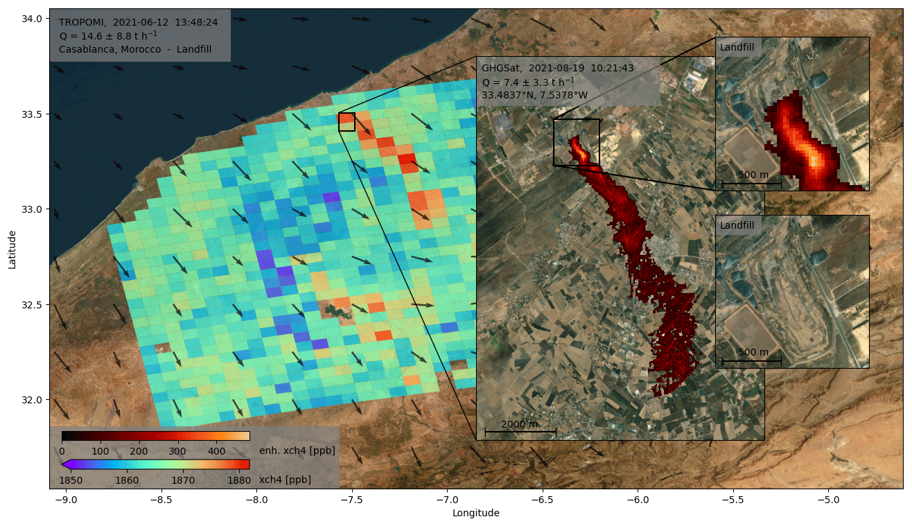
Figure 8 Methane plumes detected from Casablanca, Morocco, on 2 different days, with TROPOMI and GHGSat data overlaid over visual Esri World Imagery (Esri, Maxar, Earthstar Geographics, and the GIS User Community, 2022). Time stamps are in UTC. The plume observed by TROPOMI on 12 June 2021 is quantified at 14.6±8.8 t h⁻¹. The plume observed by GHGSat-C2 on 19 August 2021 originates from the landfill between Casablanca and Mediouna (33.483^∘ N, 7.538^∘ W) and is quantified at 7.4±3.3 t h⁻¹. The winds are the GEOS FP 10 m wind field (Molod et al., 2012).

To account for the limited TROPOMI coverage and obtain an indication of the annual emissions that our detections are representative of, we scale our detected emissions by the fraction of days with coverage. We estimate the local number of days with coverage from our 794 395 valid scenes by first mapping their spatial footprints to a 0.1×0.1^∘ grid and removing the duplicate coverage from overlapping scenes in the same orbit. We then correct for local variations in coverage (such as persistent areas without data) by convoluting this field with the summed footprints of all 2021 TROPOMI data at 0.1×0.1^∘. We finally aggregate our detected emissions to a 1×1^∘ grid and divide those by the fraction of days in 2021 with coverage resulting from the coverage map averaged to 1×1^∘. We find a scaled-up annual emission flux of 10.3 Tg, which is approximately 2.7 % of the total bottom-up 2017 anthropogenic emissions (380 Tg yr⁻¹; Saunois et al., 2020). Super-emitter plumes from landfills account for 4.1 Tg yr⁻¹ (6 % of global emissions), those from coal 2.1 Tg yr⁻¹ (4.7 %), those from oil 2.2 Tg yr⁻¹, and those of gas 1.9 Tg yr⁻¹ (4.9 % of global oil and gas; Saunois et al., 2020). These estimates are only small fractions of the total anthropogenic emissions, as our conservative upscaling approach only takes large TROPOMI-detected super-emitter plumes into account. Emissions from smaller point sources and area sources make a large contribution to the total but are not part of our upscaling. Such emissions are better captured by an atmospheric inversion.

3.2 Synergy of automated TROPOMI detections with high-resolution instruments

We use the detection of persistent methane plumes in TROPOMI data to target high-resolution observations (GHGSat-C1 and GHGSat-C2) and data analysis (PRISMA archive and Sentinel-2), following Maasakkers et al. (2022b). Furthermore, we investigate large transient emissions with data from non-targeted instruments, such as Sentinel-2.

Figure 8 shows a TROPOMI plume (14.6±8.8 t h⁻¹) detected near Casablanca in Morocco on 12 June 2021. We detected 23 plumes in the area in 2021, with source rates ranging from 8.9±5.1 to 40.5±18.0 t h⁻¹, with a mean of 18.8 t h⁻¹, indicating a persistent source (Fig. 7f). Based on a wind rotation analysis (Maasakkers et al., 2022b), we find the landfill located in between Casablanca and Mediouna to be the optimal target for high-resolution observations. Based on this TROPOMI analysis, we observe this location. The inset image shows a targeted GHGSat-C2 observation on 19 August 2021, which indeed shows a methane plume (quantified at 7.4±3.3 t h⁻¹) originating from the landfill and extending downwind.

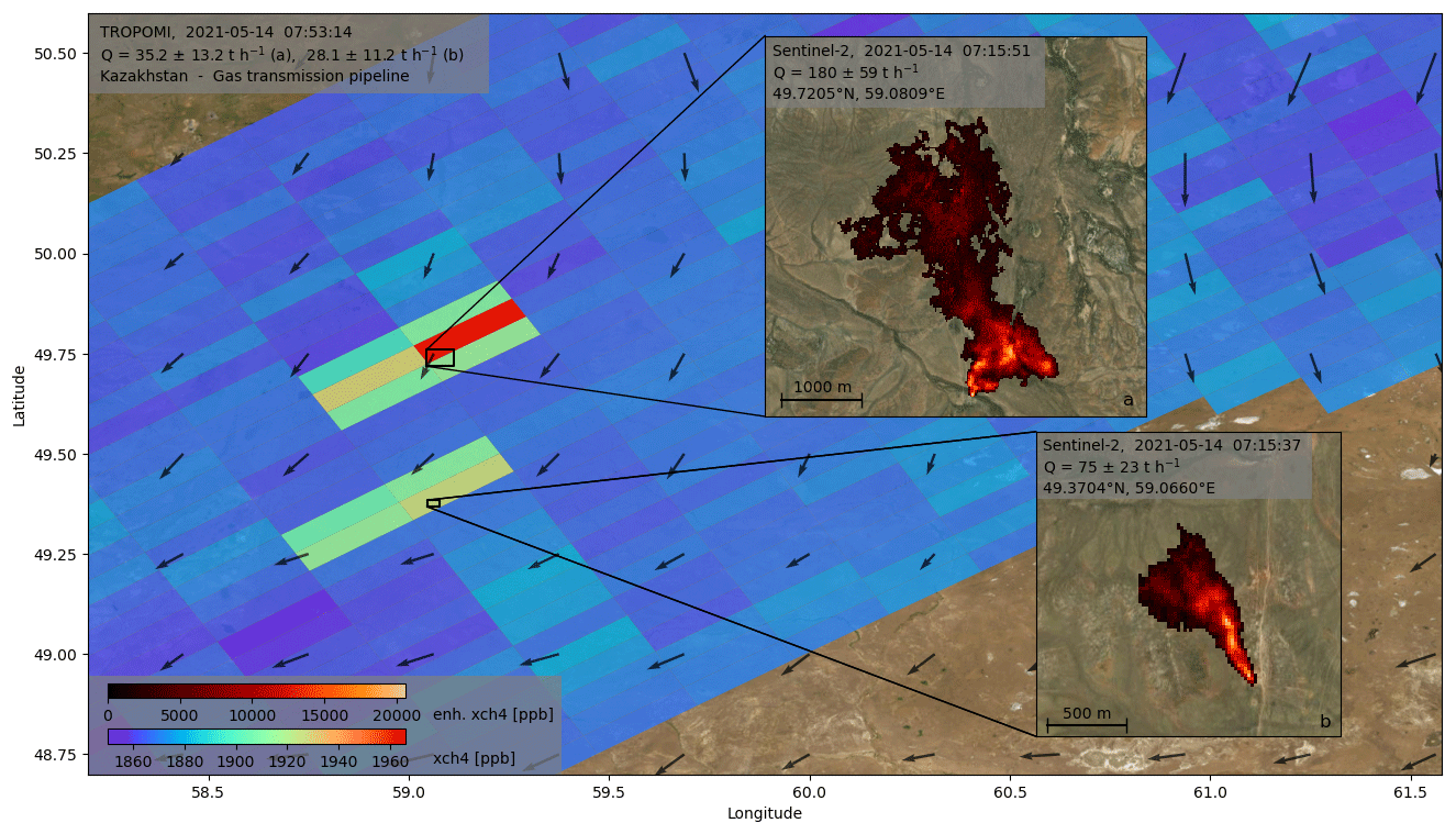
Figure 9 Transient methane plumes detected at two different locations in northern Kazakhstan, with TROPOMI (quantified at 35.2±13.2 t h⁻¹ for the northern and 28.1±11.2 t h⁻¹ for the southern plume) and Sentinel-2 overlaid over visual Esri World Imagery (Esri, Maxar, Earthstar Geographics, and the GIS User Community, 2022). Time stamps are in UTC. The plumes originate from natural gas pipeline infrastructure. The winds are the GEOS FP 10 m wind field.

Figure 9 shows two methane plumes detected with TROPOMI in northern Kazakhstan on 14 May 2021 at 07:53 UTC, quantified at 35.2±13.2 t h⁻¹ for the northern plume and 28.1±11.2 t h⁻¹ for the southern plume. The same locations were also detected in an adjacent orbit at 09:33 UTC, but the closest days with coverage before and after 14 May 2021 do not show emissions, which indicates that the plumes are transient. The bottom-up inventories show natural gas systems as being the locally dominant anthropogenic source sector because of the presence of a gas transmission pipeline. In Sentinel-2 observations taken 38 min before the first detection, we find two emitting locations close to the pipeline in the upwind part of the TROPOMI plume masks. The source rates of the Sentinel-2 plumes are 180±59 and 75±23 t h⁻¹ for the northern and southern plume, respectively. The rather large discrepancy between the TROPOMI and Sentinel-2 quantifications can be explained by the uncertain low wind speeds, the not well-developed plume in TROPOMI increasing the uncertainty in the IME, and possibly the partial pixel enhancement effect described by Pandey et al. (2019).

Figures 8 and 9 show how TROPOMI detections can be combined with high-resolution observations for both persistent and transient emitters. Figure 10 shows 10 additional locations analyzed with GHGSat (seven scenes), PRISMA (two), and Sentinel-2 (one), based on TROPOMI detections. These 12 selected locations show the range of typical anthropogenic source types and intermittencies we have observed with both TROPOMI and high-resolution instruments. Tables B1–B3 in the Supplement provide details on these high-resolution observations and associated (not necessarily on the same day) TROPOMI scenes (Table B4). We find facility-level source rates from 0.3±0.1 t h⁻¹ up to 16±5 t h⁻¹. Because of the different spatial footprints, sensitivities, and detection dates, these emission rates cannot be directly compared to the TROPOMI emission estimates (Maasakkers et al., 2022b).

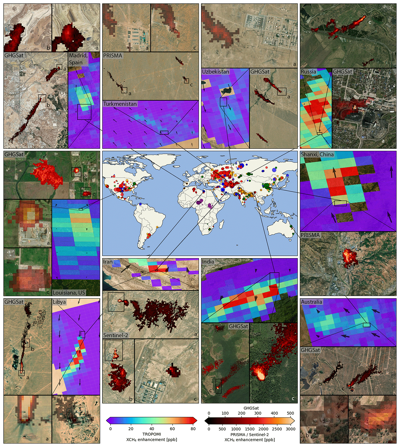
Figure 10 Plumes detected over 10 locations which were inspected with high-resolution instruments. Observations at the same location with different instruments are most often not on the same day. Details are provided in Tables B1–B3 for the high-resolution instruments and in Table B4 for TROPOMI. TROPOMI data are shown in a Mercator projection (EPSG:4326), and high-resolution data are shown in the local Universal Transverse Mercator (UTM) projection. The data are overlain over visual Esri World Imagery (Esri, Maxar, Earthstar Geographics, and the GIS User Community, 2022). The world map at the center of the image corresponds to Fig. 6, showing all 2974 detected plumes in 2021. TROPOMI data are here displayed as enhancements relative to the median $X_{{\mathrm{CH}}_{\mathrm{4}}}$ of the 32×32 pixel scene. Several of the zoomed-in views with high-resolution data were set to an opacity of 0.5 in order to reveal the infrastructure at the source of the plume.

The different specifications of the high-resolution instruments make them suitable for different purposes. The methane-designated GHGSat-Cx instruments have the lowest detection limit and are capable of retrieving methane over areas with challenging surface structures, such as urban areas. Southeast of Madrid, we observe plumes from two separate landfills located 7 km apart. The methane plumes originate from the active areas of the landfills where waste is added. In TROPOMI, the signals from these two landfills appear as a single point source. In the gas production region around Shreveport, Louisiana, USA, we observe three emission plumes originating from distinct infrastructure, including from two facilities that are only ∼500 m apart. Over a coal mining area in Russia, we see in a GHGSat observation that a single TROPOMI-based target has contributions from 10 different point sources, with source rates from 0.2±0.1 to 2.4±1.1 t h⁻¹. The emissions originate from coal mining facilities, such as underground mine vents, adding up to 8.8 t h⁻¹. In the Assam oil and gas fields, we find five plumes adding up to 12.9 t h⁻¹, showing that the GHGSat-Cx instruments are also capable of retrieving methane plumes over non-homogeneous areas including forest and agricultural lands. We also use GHGSat to target two less challenging desert scenes with oil and gas production. A GHGSat observation over Libya shows two sources downwind of each other, and the most upwind source is an unlit flare stack. At the border of Uzbekistan and Turkmenistan (listed as Uzbekistan in Fig. 10), we find emissions at three distinct locations within a single natural gas facility, with source rates ranging from 3.6±1.0 to 6.4±1.8 t h⁻¹. These emissions appear to originate from unlit flaring stacks, similar to what Irakulis-Loitxate et al. (2022b) and Varon et al. (2019) found for other natural gas facilities in the region.

For scenes with more homogeneous surfaces or extremely large emissions, PRISMA and Sentinel-2 can also be used. The PRISMA observation in Turkmenistan shows three plumes with an aggregated emission rate of 9.0±2.9 t h⁻¹. The emissions originate from distinct pieces of gas infrastructure (quantified at 3.5±1.1, 3.0±1.0, and 2.5±0.8 t h⁻¹), and the sources are located within the footprint of a single TROPOMI pixel (the same source is shown in Figs. 2 and 5). We also use the PRISMA archive to detect a plume originating from a coal mine ventilation shaft in Liuzhuang village in Shanxi, China. Finally, we use Sentinel-2 to investigate a single location in Iran with complex observation conditions (elevation), where we only had a single TROPOMI detection in 2021. The emissions therefore appeared to be transient at first, but with Sentinel-2, we find three emission plumes ranging from 1.3±0.4 to 10.0±3.0 t h⁻¹ that originate from the same oil facility in a time span of 2 months. Extensive monitoring of a location of interest over a longer time span is feasible when using Sentinel-2 (Varon et al., 2021).

4 Conclusions

We detected methane emission plumes in 2021 TROPOMI data using an automated, machine-learning-based pipeline. We have trained a convolutional neural network with a relatively small set of manually identified plumes in pre-2021 TROPOMI methane data to detect plume-like morphological structures (κ score of 0.97 and recall of 0.98 on the test set). We then used a support vector classifier to distinguish real plumes from retrieval artifacts using additional information from the scene and supporting data (κ score of 0.81 and recall of 0.93 on the test set). This two-step approach can also be applied to other instruments in the future. We tested our detection, source localization, and emission quantification estimate for a specific, well-characterized natural gas well blowout and found that it was accurately captured by our monitoring system. After the application of our pipeline to the 2021 data, we targeted high-resolution observations and analyses to find the facilities responsible for 12 (clusters of) plumes seen in TROPOMI.

Using our automated machine learning pipeline, we scan all 794 395 scenes of 2021 in 3 h on a single core. Of these scenes, 4869 are automatically classified as plumes, of which 2974 are manually verified as being confident plumes and 745 as being potential plumes, thus giving the automated pipeline a precision of 61 %–76 %. The most challenging distinction for the SVC is between plumes and artifacts, which is a distinction that can be inconclusive even for a human expert in difficult cases. We focus on the manually verified plumes; the remaining 39 % of the scenes are mostly difficult to classify and can still be followed up with manual inspection or be used to further train the models. We find that most plumes (74.8 %) originate from 94 clusters of detections around both known and new, persistent source locations. The other plumes are mainly caused by transient emission events, such as along natural gas transmission pipelines in Russia. We most often detect plumes (based on bottom-up emission inventories) from urban areas and/or landfills (1031 plumes), followed by 720 plumes from gas infrastructure, 612 from oil infrastructure, and 581 from coal mining. Many of the identified clusters are located at well-known fossil fuel exploitation regions or urban areas known to emit methane. We also identify several previously unstudied sources such as in Libya and Assam (India) and identify specific super-emitting locations within spread-out fossil fuel production regions like the Shanxi coal mining area in China. Based on IME quantifications of all plumes, we found mean emissions of 44 t h⁻¹ with a 5–95th percentile range of 8–122 t h⁻¹, which is an indication of the TROPOMI detection limit. With 1143 detections under 25 t h⁻¹, including 241 plumes under 10 t h⁻¹, our automated approach has a better detection limit than previously published methods based on TROPOMI data. When we assume that all 2944 detected anthropogenic emissions are active for 24 h, we find detected 2021 emissions of 3.1±1.3 Tg. Accounting for the limited coverage of TROPOMI, these detected emissions are representative of 10.3 Tg yr⁻¹, which is approximately 2.7 % of global annual anthropogenic methane emissions.

For 12 locations, we used high-resolution satellite observations (GHGSat-C1 and GHGSat-C2, PRISMA, and Sentinel-2) to identify the exact sources responsible for the detected plumes in TROPOMI. We utilized the different strengths of the high-resolution instruments; we made targeted observations with GHGSat over scenes with complex surface reflectance, whereas the archive of Sentinel-2 is used to analyze large transient emission events and track intermittent emissions. We found point sources from landfills and fossil fuel exploitation with emission rates from 0.3±0.1 to 180±59 t h⁻¹. Most fossil-fuel-related TROPOMI plumes had contributions from multiple point sources, with one GHGSat observation over Russia revealing emissions from 10 different sources.

Over the next few years, the number of global, regional, and point source mapping instruments capable of retrieving methane plumes will vastly increase, including Sentinel-5, CO2M, MethaneSAT, and Carbon Mapper (Jacob et al., 2022). Our monitoring system can incorporate these fast-growing data volumes and can already be used to automatically detect plumes in the operational TROPOMI data, track temporal variability in super-emitter plumes, and tip and cue high-resolution satellite instruments to find the associated super-emitting facilities. This identification and monitoring of super-emitters with large mitigation potential is paramount to reach the goals of the Global Methane Pledge.

Appendix A: CNN training data table

Table A1 An overview of the split in training and test data for the CNN (Fig. 1, CNN training).

Appendix B: Details on the plumes observed with high-resolution instruments

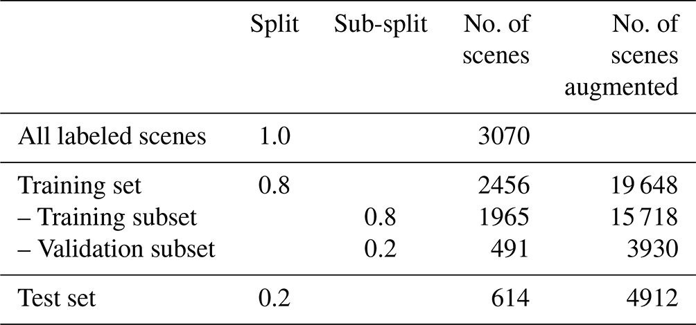
Table B1 Observation, location, and quantification details corresponding to the GHGSat scenes, one of which is in Morocco, Casablanca (landfill in Fig. 8). Wind speeds are 10 m wind speeds obtained from GEOS FP (Molod et al., 2012). Locations Uzbekistan-b and Uzbekistan-c are located just over the border in Turkmenistan; however, the main building of the facility (near Uzbekistan-a) is located in Uzbekistan. Because there is another location in Turkmenistan, we have chosen this nomenclature. Note that “O&G facility” is for oil and gas facilities.

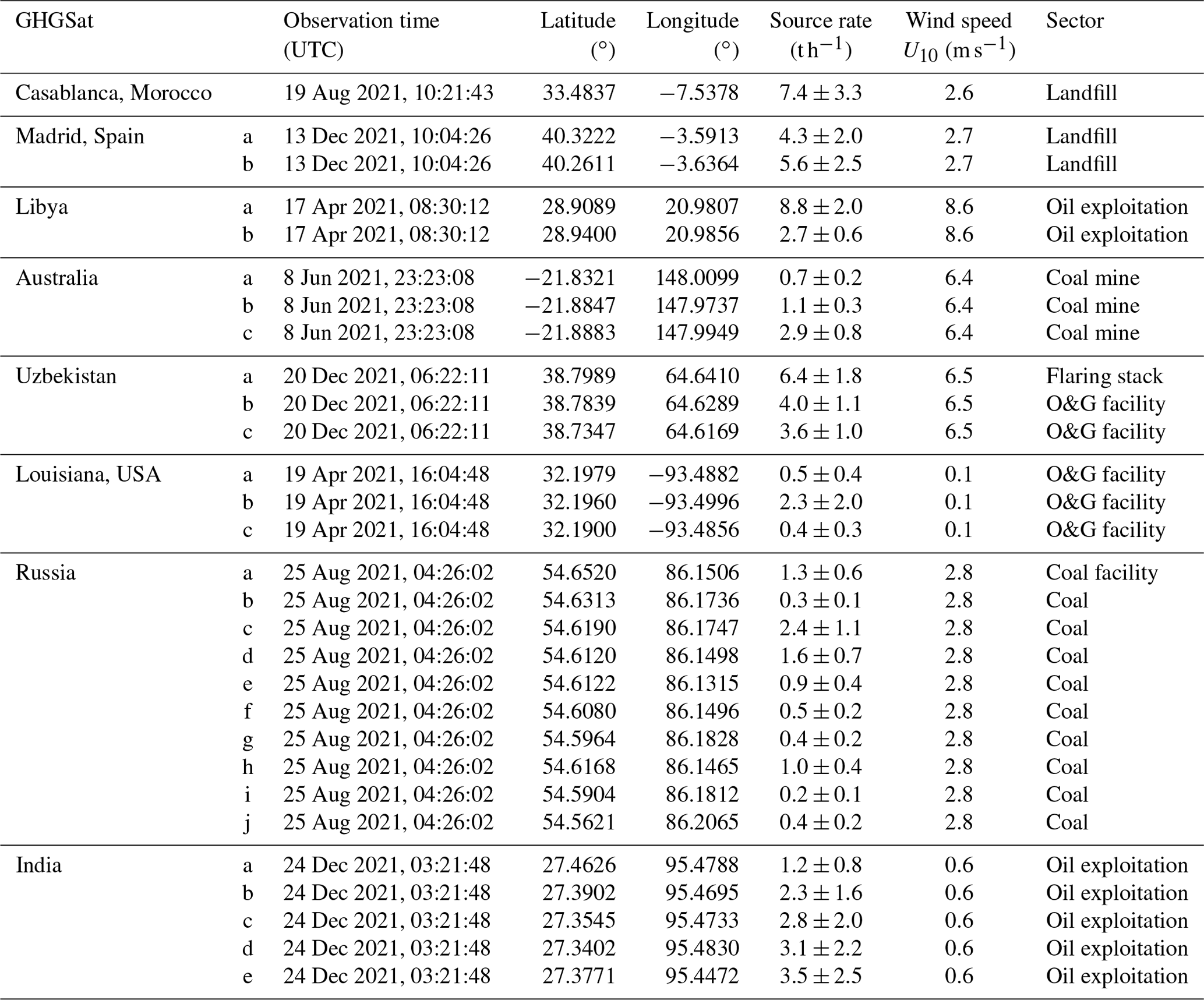
Table B2 Observation, location, and quantification details corresponding to the PRISMA scenes. Wind speeds are 10 m wind speeds obtained from GEOS FP (Molod et al., 2012). The plume mask of plume Turkmenistan-c (Fig. 10; Table B2) was curated in order to exclude an artifact which was caused by a nearby road. Retrieval artifacts in high-resolution methane retrievals from hyperspectral instruments resulting from surface features such as roads is a known issue (Sánchez-García et al., 2022; Gorroño et al., 2023). PRISMA and Sentinel-2 are more prone to such issues than GHGSat-Cx. Note that “O&G facility” is for oil and gas facilities.

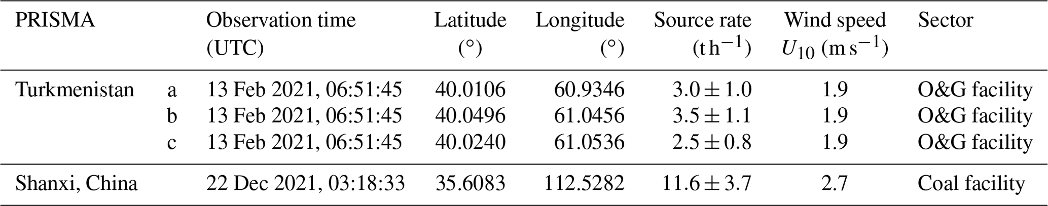
Table B3 Observation, location, and quantification details corresponding to the Sentinel-2 scenes, one of which is Kazakhstan (natural gas pipeline in Fig. 9). Wind speeds are 10 m wind speeds obtained from GEOS FP (Molod et al., 2012).

Table B4 Observation, location, and quantification details of the TROPOMI scenes corresponding to the high-resolution observations in Figs. 8–10. Wind speeds presented in this table are the GEOS 10 m, GEOS PBL, and ERA5 10 m wind products (Molod et al., 2012; Hersbach et al., 2020), which are used to compute three U_eff values, which are then averaged (Sect. 2.5.1).

Appendix C: Features used as input for the SVC

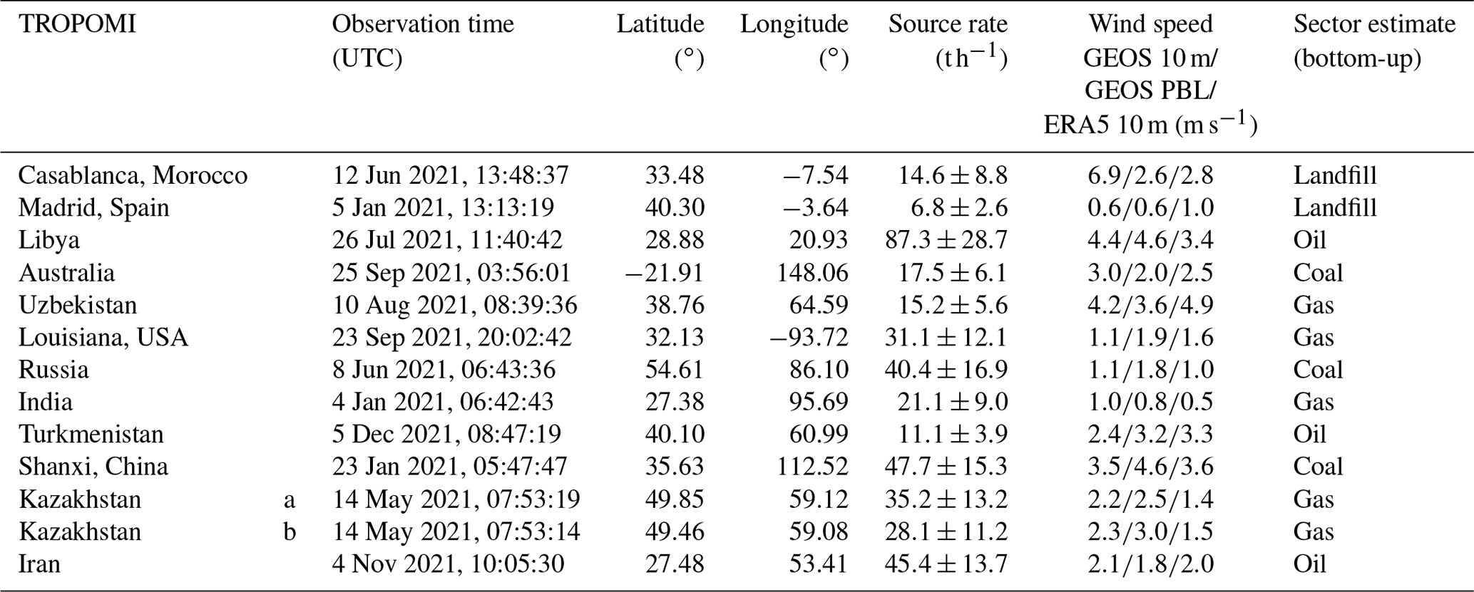
Table C1 Overview of the features used by the SVC as input. Each scene is represented as a feature vector with a shape (1×41). This table provides the name of the feature, the category the feature is aiming to provide information about, the ranking of the top 10 features in the feature importance analysis (FIR is the feature importance ranking), the possible range of values the feature can attain, and a description of the feature. Note that AOT is for aerosol optical thickness, and QA is for quality assurance.