Can we use atmospheric CO₂ measurements to verify emission trends reported by cities? Lessons from a 6-year atmospheric inversion over Paris

Existing CO₂ emissions reported by city inventories usually lag in real-time by a year or more and are prone to large uncertainties. This study responds to the growing need for timely and precise estimation of urban CO₂ emissions to support present and future mitigation measures and policies. We focus on the Paris metropolitan area, the largest urban region in the European Union and the city with the densest atmospheric CO₂ observation network in Europe. We performed long-term atmospheric inversions to quantify the citywide CO₂ emissions, i.e., fossil fuel as well as biogenic sources and sinks, over 6 years (2016–2021) using a Bayesian inverse modeling system. Our inversion framework benefits from a novel near-real-time hourly fossil fuel CO₂ emission inventory (Origins.earth) at 1 km spatial resolution. In addition to the mid-afternoon observations, we attempt to assimilate morning CO₂ concentrations based on the ability of the Weather Research and Forecasting model with Chemistry (WRF-Chem) transport model to simulate atmospheric boundary layer dynamics constrained by observed layer heights. Our results show a long-term decreasing trend of around 2 % ± 0.6 % per year in annual CO₂ emissions over the Paris region. The impact of the COVID-19 pandemic led to a 13 % ± 1 % reduction in annual fossil fuel CO₂ emissions in 2020 with respect to 2019. Subsequently, annual emissions increased by 5.2 % ± 14.2 % from 32.6 ± 2.2 Mt CO₂ in 2020 to 34.3 ± 2.3 Mt CO₂ in 2021. Based on a combination of up-to-date inventories, high-resolution atmospheric modeling and high-precision observations, our current capacity can deliver near-real-time CO₂ emission estimates at the city scale in less than a month, and the results agree within 10 % with independent estimates from multiple city-scale inventories.

1 Introduction

Most countries have actively committed to the 2015 Paris Agreement in order to limit global warming to well below 2 ^∘C, preferably to 1.5 ^∘C, compared with pre-industrial levels. To achieve this goal, governments have pledged to implement stringent climate actions to reduce their national emissions with the ultimate objective of reaching climate neutrality by 2050. Cities account for more than 70 % of annual global fossil fuel CO₂ emissions and are thus key areas for mitigating CO₂ emissions (Seto et al., 2014). To date, many metropolitan areas have pledged to reduce CO₂ emissions and have begun to implement policies to achieve net-zero emissions (e.g., C40 Cities, Global Covenant of Mayors for Climate & Energy). The choice of mitigation actions, for cost-effectiveness and to maximize the emission reduction impact, mainly depends on the qualitative and quantitative knowledge of urban emission sources with temporal–spatial characteristics in order to understand evolving emission trends (Lauvaux et al., 2020; Mueller et al., 2021). However, the bottom-up carbon emissions based on public protocols for cities are prone to large uncertainties (Gurney et al., 2021). High-resolution gridded CO₂ emission inventories, e.g., the Hestia dataset for some US cities (Gurney et al., 2019) or the London Atmospheric Emissions Inventory (LAEI) dataset for Greater London (Greater London Authority, 2021), provide detailed descriptions of emissions from urban domains. This approach relies on a collection of extensive activity data and emission factors and can thus be labor-intensive and time-consuming, especially when doing regular updates. Recently, Carbon Monitor Cities has been developed to provide near-real-time city-level CO₂ emissions data for 1500 global cities from 2019 to 2021 (Huo et al., 2022).

The quantification of greenhouse gas (GHG) emissions from atmospheric measurements offers accounting complementary to the conventional bottom-up approach (Ciais et al., 2010). These methods combine atmospheric measurements with bottom-up inventories through inversion techniques (Tarantola, 2005). Scientific capabilities evolve rapidly with increasing model performances (Deng et al., 2017) and the deployment of dense networks in cities, e.g., the Washington DC–Baltimore metropolitan areas (Karion et al., 2020), the San Francisco Bay Area (Turner et al., 2020), Los Angeles (Yadav et al., 2021), Indianapolis (Davis et al., 2017), Paris, Munich and Zurich (https://www.icos-cp.eu/projects/icos-cities, last access: August 2023). The robustness of the inversion and the derived emission estimates need to be evaluated over periods of several months and years in order to check the stability and relevance of the seasonal cycle and the interannual variability. For example, McKain et al. (2012) indicated that their transport model showed a poor performance in modeling urban sites such that only relative changes in the emission estimates were considered relevant. To our knowledge, few estimates of city GHG emissions based on long-term tower-based measurements and atmospheric inversion systems have been published. These include studies covering a period over 1 to 5 years for the cities of Paris, Boston, Indianapolis and Los Angeles (Staufer et al., 2016; Sargent et al., 2018; Lauvaux et al., 2020; Yadav et al., 2023).

The Paris region, known as Île-de-France (IdF), is the most densely populated and most economically active region in France. Covering only 2 % of French territory, it is inhabited by around 18 % of the French population (12.2 out of 67.8 million inhabitants) and produces 31 % of the national gross domestic product (GDP) and 10 % of human-caused GHG emissions of France (source: AirParif, https://www.airparif.asso.fr/en/monitor-pollution/emissions, last access: August 2023; CITEPA, https://www.citepa.org/fr/2022-co2e/, last access: August 2023). Paris is one of the most active cities in tackling climate change and is part of the C40 Cities consortium. The first Paris Climate Plan was adopted in 2007 and targeted a 25 % reduction in GHG emissions by 2020 with respect to 2004 levels. Paris also has an ambitious 2020–2030 action plan which targets a 50 % decrease in local direct GHG emissions (Scope 1) compared with 2004 levels (Le Plan Climat de Paris, 2020). According to the AirParif (official air-quality agency of the Paris region; https://www.airparif.asso.fr/en/, last access: August 2023) inventory, the contribution of each of the main GHGs (in terms of CO₂-equivalent emissions) was 94 % for CO₂, 4 % for N₂O and 2 % for CH₄ in 2010 (AirParif, 2013). Regarding atmospheric CO₂ monitoring capability, Paris is an important pilot city with the densest and most comprehensive atmospheric CO₂ measurements in Europe (e.g., Lopez et al., 2013; Xueref-Remy et al., 2018; Vogel et al., 2019; Lian et al., 2019). The Parisian ground-based network, whose first measurements date back to 2010, has grown from an initial three to the current seven high-precision continuous in situ CO₂ monitoring stations. Over the past few years, a series of studies have attempted to analyze the spatial–temporal variations in CO₂ concentrations over the Paris region and have tried to monitor fossil fuel CO₂ emissions through an atmospheric inversion technique (Bréon et al., 2015; Wu et al., 2016; Staufer et al., 2016). Lian et al. (2022) estimated CO₂ emission reductions during COVID-19 confinements in Paris, which demonstrated the capability of the urban atmospheric monitoring system to identify significant emission changes (>20 %) at short-term monthly timescales.

This study performs the first long-term atmospheric CO₂ inversions over the Paris metropolitan area and compares it with multiple city-scale inventories. It aims at assessing the robustness of the inversion and its ability to track absolute urban CO₂ emission levels, as well as the relative changes in these emissions over multiple years. The 6-year (2016–2021) continuous CO₂ measurements in Paris now provide sufficient information to investigate the variations in CO₂ emissions at different timescales (daily, seasonal and interannual) across an urban area. In addition to the mid-afternoon CO₂ concentration measurements that are commonly used for inversions, we also explore the potential of assimilating morning CO₂ data, taking into account the performance of the Weather Research and Forecasting model with Chemistry (WRF-Chem; Grell et al., 2005) in capturing the evolution of the atmospheric boundary layer (ABL) dynamics. The height of the ABL is the main driver of uncertainties when assessing emissions from concentrations. This paper is organized as follows: Sect. 2 provides details of the city-scale Bayesian inversion methodology. Section 3 shows the variations in CO₂ emissions at different timescales. Section 4 summarizes the main conclusions and perspectives for further research.

2 Methods

A city-scale Bayesian inversion was conducted to quantify CO₂ emissions over a 6-year period spanning January 2016 to December 2021. The inversion system is based on atmospheric CO₂ measurements at seven in situ stations combined with meteorological measurements, the WRF-Chem transport model run at 1 km×1 km horizontal resolution (Lian et al., 2021), a near-real-time fossil fuel CO₂ inventory produced by Origins.earth, and the biogenic CO₂ fluxes simulated by the Vegetation Photosynthesis and Respiration Model (VPRM) included in WRF-Chem (Mahadevan et al., 2008). Details regarding the inversion system setup are described in Lian et al. (2022) and are outlined briefly below.

2.1 CO₂ measurement network

The seven stations are equipped with high-precision cavity ring-down spectroscopy (CRDS) CO₂ analyzers, together with an automated data processing and quality-control system. CO₂ observations are calibrated every 1 to 6 months with standards traceable to the World Meteorological Organization (WMO) CO₂ X2019 calibration scales (Hall et al., 2021). The precision of the 1 h average CO₂ concentration is better than 0.1 ppm (Xueref-Remy et al., 2018). These stations are roughly distributed along a northeast–southwest axis of the Paris urban area, which coincides with the predominant wind directions (Fig. 1).

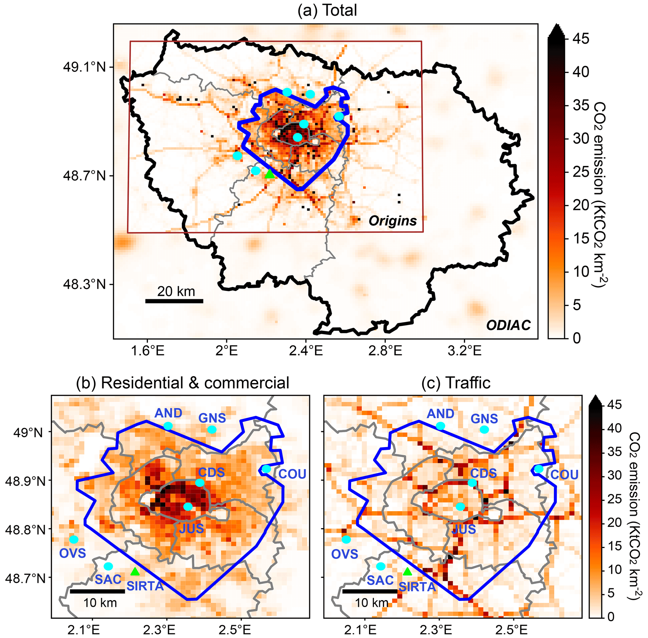
Figure 1 Distributions of annual (a) total fossil fuel emissions, (b) residential and commercial emissions, and (c) traffic CO₂ emissions for the year 2019 according to the Origins.earth inventory (brown rectangle) complemented by the ODIAC dataset. The seven in situ CO₂ measurement stations are shown in cyan circles. The location of the SIRTA observatory with ABL measurements is marked by a green triangle. The bold black line shows the administrative limits of the Île-de-France (IdF) region. In the inversion system, emissions over two emitting regions are optimized: the greater Paris region (within the blue line) and the rest of the IdF region.

Figures 2 and S1 in the Supplement show the monthly and daily average daytime (08:00–17:00 UTC) CO₂ concentrations at each in situ station from 2016 to 2021, respectively, and in addition Fig. 2 also shows the simulated background CO₂ concentration at the SAC station using the Copernicus Atmosphere Monitoring Service (CAMS) CO₂ dataset as the boundary and initial inputs for WRF-Chem. The atmospheric background CO₂ concentrations have steadily been rising over the past 6 years, which is primarily attributed to global human activities. Generally, the average CO₂ concentrations across the network vary seasonally between 390 and 450 ppm. They are mainly driven by the atmospheric transport, the CO₂ biospheric cycle and their proximity to the urban anthropogenic CO₂ emission sources. The interannual CO₂ variations primarily depend on the year-to-year variations in synoptic weather conditions, air temperature and the associated emissions. For example, the notably high CO₂ concentrations observed near the surface during the 2016/17 winter were caused by stagnant, often stable, atmospheric stratification associated with cold and dry air masses and low-ventilation weather conditions over the north of France (Bulletin Climatique Météo-France, 2016, 2017).

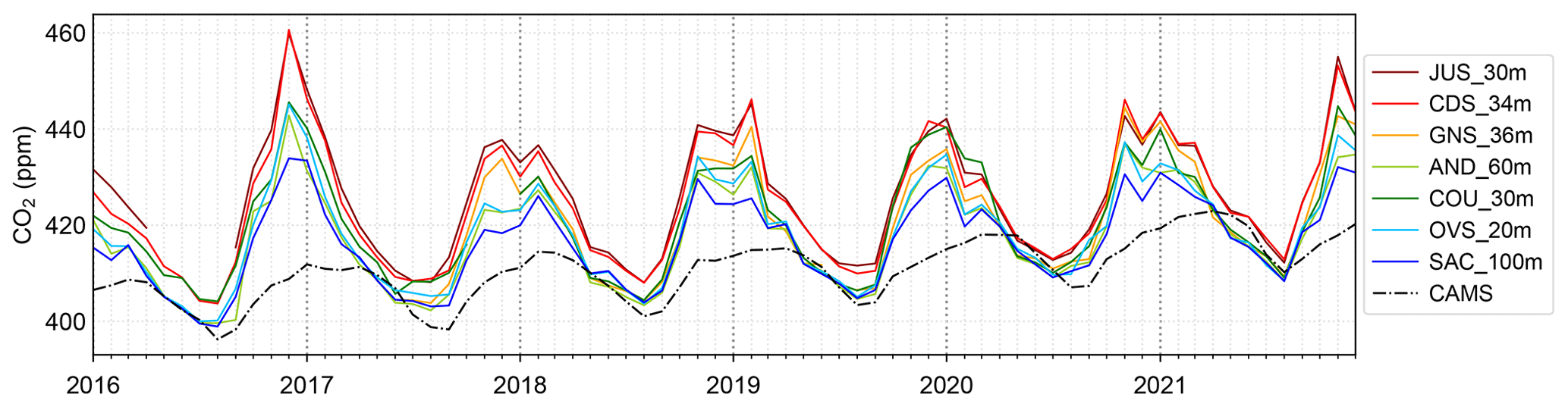
Figure 2 Monthly average daytime-observed (08:00–17:00 UTC) CO₂ concentrations at seven in situ stations. The dashed black line indicates the simulated background CO₂ concentration over Paris by WRF-Chem driven by the CAMS global atmospheric CO₂ dataset. The sampling heights above ground level are given in the legend.

The gradients of CO₂ concentrations between the downwind and upwind stations are linked to the emissions within the Paris urban area. The CO₂ concentrations are significantly higher at the two urban stations CDS and JUS than those at peri-urban sites across all seasons (Fig. 2). The magnitude in CO₂ gradients between urban and suburban areas is around 5–10 ppm in summer, increasing to 20–30 ppm during the winter months as a result of more stable atmospheric conditions (lower vertical dispersion and shallow ABL height) combined with high emissions from residential heating. The citywide CO₂ gradients across the Paris agglomerations have shown their potential in previous inversion studies to estimate the city-scale CO₂ emissions (Bréon et al., 2015; Staufer et al., 2016).

2.2 Origins.earth and other CO₂ inventories

Fossil fuel CO₂ a priori fluxes used in this study are taken from a patent pending a high-resolution inventory produced by Origins.earth (https://www.origins.earth/, last access: August 2023) over the IdF region, in combination with the global Open-source Data Inventory for Anthropogenic CO₂ (ODIAC) product (Oda et al., 2018) in surrounding areas. The Origins.earth bottom-up inventory is a gridded map of fossil fuel CO₂ emissions within a rectangular (on a latitude and longitude grid) domain which encompasses most of the IdF region (Fig. 1) at a 1 km×1 km spatial and hourly temporal resolution. It has provided the Scope 1 CO₂ emissions from the year 2018 until the present time. For the simulation period from 2016 to 2017, we used CO₂ emissions from the Origins.earth inventory for the year 2018 as the WRF-Chem model inputs. The Origins.earth inventory includes more than 60 source types for carbon emission activities. These types of activities are grouped into six activity sectors (e.g., transportation, residential, tertiary, industrial (including cement), energy and waste sectors). The inventory compilation method is outlined in the Supplement (Text S1).

The IdF is a large urban region with estimated annual fossil fuel CO₂ emissions exceeding 30 Mt CO₂ yr⁻¹, dominated by traffic and residential sectors. The spatial distributions of the emissions are shown in Fig. 1. According to the Origins.earth inventory, the annual emission budgets of the residential sector are 11.0, 10.9, 10.1 and 11.4 Mt CO₂, representing 32 %, 34 %, 35 % and 38 % of total emissions for 2018, 2019, 2020 and 2021, respectively. For the traffic sector, averages are 12.3 Mt CO₂ (36 %), 10.9 Mt CO₂ (33 %), 8.7 Mt CO₂ (30 %) and 8.7 Mt CO₂ (29 %) from 2018 to 2021 (Fig. S2b). Figure S2a shows the daily fossil fuel CO₂ emissions by sector and their respective proportions from 2018 to 2021. Generally, the temporal variations in CO₂ emissions from the building sector show a large seasonal cycle, mainly related to the heating demand that is linearly driven by the variations in air temperature below a threshold of ≈19 ^∘C. Emissions from the tertiary, industrial and energy sectors have a relatively flat seasonal variation.

In this study, the inverse emissions are compared with independent estimates from different inventories and a published study. These include (i) the TNO-GHGco inventory at a resolution of $\mathrm{1}/\mathrm{10}{}^{\circ }\times \mathrm{1}/\mathrm{20}{}^{\circ }$ (long × lat) ($\sim \mathrm{6}\mathrm{km}\times \mathrm{6}\mathrm{km}$) for the years 2005–2020 (Denier van der Gon et al., 2021); (ii) the TNO-GHGco inventory at a resolution of $\mathrm{1}/\mathrm{60}{}^{\circ }\times \mathrm{1}/\mathrm{120}{}^{\circ }$ (long × lat) ($\sim \mathrm{1}\mathrm{km}\times \mathrm{1}\mathrm{km}$) for the years 2015, 2017, and 2018 (Dellaert et al., 2019); (iii) the AirParif inventory developed by the local official air-quality agency at a 1 km×1 km resolution for the years 2005, 2010, 2015, and 2018, (iv) the city-level CO₂ emissions from the Carbon Monitor Cities dataset (https://cities.carbonmonitor.org/, last access: August 2023, Huo et al., 2022) for the years 2019–2021; and (v) the study by Staufer et al. (2016), who reported a full year's (August 2010–July 2011) estimate of the IdF region fossil fuel CO₂ emissions by assimilating citywide CO₂ measurements from a sparse network of three stations with the inversion methodology. Here, we consider that these multiple emission estimates allow for a cross-validation as they were developed by several research groups using distinct data sources, methods and protocols.

2.3 Adding morning CO₂ data and ABL height selection

The accuracy of atmospheric inversion results depends to a large extent on the quality of the atmospheric transport model. The major uncertainties in CO₂ modeling are related to model errors in horizontal wind and vertical mixing within the atmospheric boundary layer (Kretschmer et al., 2012). A stringent data selection of CO₂ concentrations to be assimilated for the inversion is generally applied (e.g., Staufer et al., 2016; Wu et al., 2016; Lauvaux et al., 2020). The aim of the data selection is to rule out observations that are difficult to simulate accurately with the transport model. Previous studies (Staufer et al., 2016; Lian et al., 2022) have assimilated only afternoon CO₂ data from 12:00 to 17:00 UTC, during which the atmospheric boundary layer is expected to be well developed. Moreover, the wind speeds at downwind stations are required to be higher than 3 m s⁻¹ to minimize possible contaminations from local sources of CO₂ emissions near the measurement sites that cannot be reproduced by the model.

However, the selection of a limited number of suitable data produces more uncertain estimates over periods when no observations are selected. The high sensitivity of the inverse emissions to the diurnal variations in prior emissions also highlights the limitations induced by assimilating data only during the afternoon. Therefore, we attempt to include morning CO₂ concentration data in this study. Given that atmospheric models have difficulties in correctly reproducing the mixing processes under stable conditions and when the boundary layer develops in the morning, caution is required when assimilating morning CO₂ concentrations. We assumed that the ABL height could provide a good diagnostic to assess the vertical mixing and dilution associated with turbulence near the surface. We thus first evaluated the WRF-Chem-simulated ABL heights against observations at the SIRTA station (Haeffelin et al., 2005) located about 20 km southwest of the center of Paris (Fig. 1). The modeled ABL heights were diagnosed from the potential temperature using the 1.5-theta-increase method (Nielsen-Gammon et al., 2008), while the aerosol-based STRATfinder algorithm (Kotthaus et al., 2020) was applied to derive ABL heights from attenuated backscatter profiles measured with an automatic lidar ceilometer (Lufft CHM 15k).

Figure S3 shows hourly ABL heights derived from both measurements and simulations from 2016 to 2021 for morning (08:00–11:00 UTC) and afternoon (12:00–17:00 UTC) periods, respectively. In general, the model captures the ABL heights throughout the year with a fair correlation coefficient (>0.6) reasonably well. However, the simulated ABL heights are, on average, higher than the measurements with biases of 80–130 m. This could reflect an overestimation of the atmospheric instability in the lowest atmospheric layer by WRF or may in fact indicate that vertical dilution of atmospheric tracers (here observed aerosol profiles) may lag behind the thermodynamic evolution of the ABL morning development (Text S2). Particularly large relative discrepancies are detected during the winter and morning periods associated with stable atmospheric conditions. This model–observation comparison of ABL heights allows us to revise the recent selection of CO₂ concentration measurements that can be assimilated into the inversion system as used in Lian et al. (2022) and to extend it into the morning period (Fig. S4). The revision consists primarily of adding two additional selection criteria concerning the morning data between 08:00–11:00 UTC. First, we discard the data when the relative error of the modeled ABL heights against observations is larger than 80 %. This threshold was set based on the distributions of the relative errors in ABL shown in Fig. S3. Second, we apply a tighter filtering for the morning data (08:00–11:00 UTC) by increasing the minimum wind speed threshold to 5 m s⁻¹ compared with the 3 m s⁻¹ used for the afternoon.

2.4 Inversion configuration

The main principle of the Bayesian atmospheric inversion presented in Lian et al. (2022) is to optimize the 6 h mean fossil fuel CO₂ emission budgets of the greater Paris region (within the blue line in Fig. 1) and the rest of the IdF region over four time windows per day (00:00–05:00, 06:00–11:00, 12:00–17:00, 18:00–23:00 UTC). The approach assimilates atmospheric CO₂ concentration gradients between pairs of stations located upwind and downwind of the city to decrease the uncertainties caused by the transport of remote and natural fluxes outside the urban area. The configurations of the atmospheric inversion system in this study are described in detail in Lian et al. (2022). The configurations comprise the setup of the control vectors, the selection of the assimilated downwind–upwind CO₂ observation gradients (Fig. S4), the assignments of the observation error and the prior flux uncertainties. Compared with Lian et al. (2022), only two minor modifications are made in this study in order to assess the impacts of morning CO₂ concentrations on the retrieved emissions. (1) Regarding the fossil fuel emissions, we assume a 60 % relative uncertainty in the prior estimates of individual 6 h emission budgets. (2) We assign no temporal correlation of prior uncertainties between the different 6 h time windows. The data selection criteria of the assimilated CO₂ observations and the assignments of the prior flux uncertainties of the reference inversion are shown in Table S1 in the Supplement. In addition, we also conducted a series of sensitivity tests to investigate how the inverse estimates respond to changes in various setups of the inversion system (Table S1). This inversion ensemble was composed of five tests of the selection criteria of the assimilated CO₂ observations as well as five tests of the uncertainties and the temporal correlations of the prior emissions.

3 Results

3.1 Daily emission estimates

Statistical comparisons between the assimilated modeled and measured CO₂ concentration gradients before and after flux optimizations are shown in Fig. S5. In general, the inversion leads to an overall improvement in the representation of observations, for both the morning period (08:00–11:00 UTC) (Fig. S5c) and the afternoon period (12:00–17:00 UTC) (Fig. S5d). The mean bias errors (MBEs) are reduced from −0.85 to −0.29 ppm in the morning and from −1.16 to −0.55 ppm in the afternoon after the inversion. The selected morning CO₂ gradients correspond to ∼24.5 % (5168 of 21 091) of the total assimilated observation gradients.

Figure 3 compares the estimates from the reference inversion, which assimilates the daytime (08:00–17:00 UTC) CO₂ concentration gradients, to the estimates from the two sensitivity tests that only use morning (08:00–11:00 UTC) or afternoon (12:00–17:00 UTC) CO₂ data, respectively. Here, we mainly focus on the greater Paris region (Fig. 1) where the fossil fuel CO₂ emissions can be well constrained from our observation network. Figure 3 shows the average prior and posterior fossil fuel CO₂ emission estimates together with their associated uncertainties over the 6-year period spanning January 2016 to December 2022, for the four 6 h time windows and every day of the week. The time series of the daily prior and posterior fossil fuel CO₂ emissions are shown in Fig. 4. The reference inversion (Fig. 3b) mainly imposes a direct constraint on the fossil fuel fluxes for the two 6 h windows of the day (06:00–11:00 and 12:00–17:00 UTC), while having little constraint on nighttime emissions (00:00–05:00 and 18:00–23:00 UTC). This is because the assimilated daytime CO₂ concentrations are mainly sensitive to the emissions from the morning and afternoon periods. The inversion increases the average posterior emissions per day of the week by around 9 %–16 % and 13 %–23 % with uncertainty reductions of 14 %–21 % and 15 %–21 % for the 06:00–11:00 and 12:00–17:00 UTC time windows, respectively. The assimilation of only afternoon CO₂ data (Fig. 3d) has similar retrieved emissions but with a smaller uncertainty reduction, especially for the 06:00–11:00 UTC period, compared with the reference one which assimilates morning data. Even though we assimilate a relatively small number of morning CO₂ data (Fig. 3c), such a change still leads to a 11 %–16 % uncertainty reduction compared with a priori of the morning fossil fuel emissions (Fig. 3c).

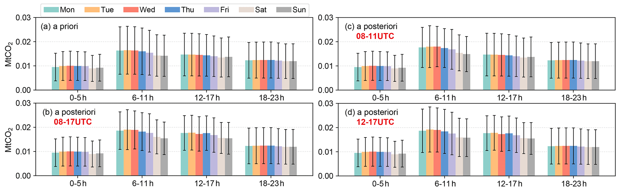
Figure 3 Average (a) prior and (b–d) posterior fossil fuel CO₂ emission estimates and their uncertainties over the greater Paris region over the years 2016–2021, for the four 6 h time windows and the days of the week. Panels (b)–(d) present the posterior CO₂ estimates when assimilating (b) daytime (08:00–17:00 UTC), (c) morning (08:00–11:00 UTC) and (d) afternoon (12:00–17:00 UTC) selected CO₂ concentration observations, respectively.

The inversion on average reduces the uncertainty in the daily fossil fuel CO₂ emission estimates (Fig. 4a) from ∼31 % (prior) down to ∼24 % ± 4.5 % (posterior) (a range of 2.5 %–11.5 % uncertainty reduction) over the greater Paris region. On the contrary, CO₂ emissions over the rest of the IdF region (Fig. S6) after the inversion remain close to their prior values due to insufficient observational constraints. The inverse CO₂ emissions show a fairly good agreement with the prior estimate with a Pearson correlation coefficient (R) of 0.91, which indicates that the Origins.earth near-real-time inventory can already capture some timely emission variations that are closely related to meteorological effects and human activities relatively well. For instance, the lower emissions in February 2020 appear to be mainly due to weather conditions, with a mild winter leading to a lower demand for heating (Bulletin Climatique Météo-France, 2020). A decrease in the daily CO₂ emissions is observed in July and August due to a reduction in traffic emissions during the summer holidays. It can also be seen that the daily fossil fuel CO₂ emissions dropped by more than 30 % in the second half of March 2020, when strict COVID-19 lockdown measures were adopted. In general, the inverse CO₂ emissions exhibit a larger daily variability compared with the prior. On the one hand, the temporal profiles used in the inventory rely on some degree of interpolation, proxy data and theoretical assumptions that can smooth out some temporal variability. On the other hand, the posterior daily variability represents both the actual variability in emissions caused by human activities and the sources of uncertainty in the inverse modeling system, especially the transport model errors.

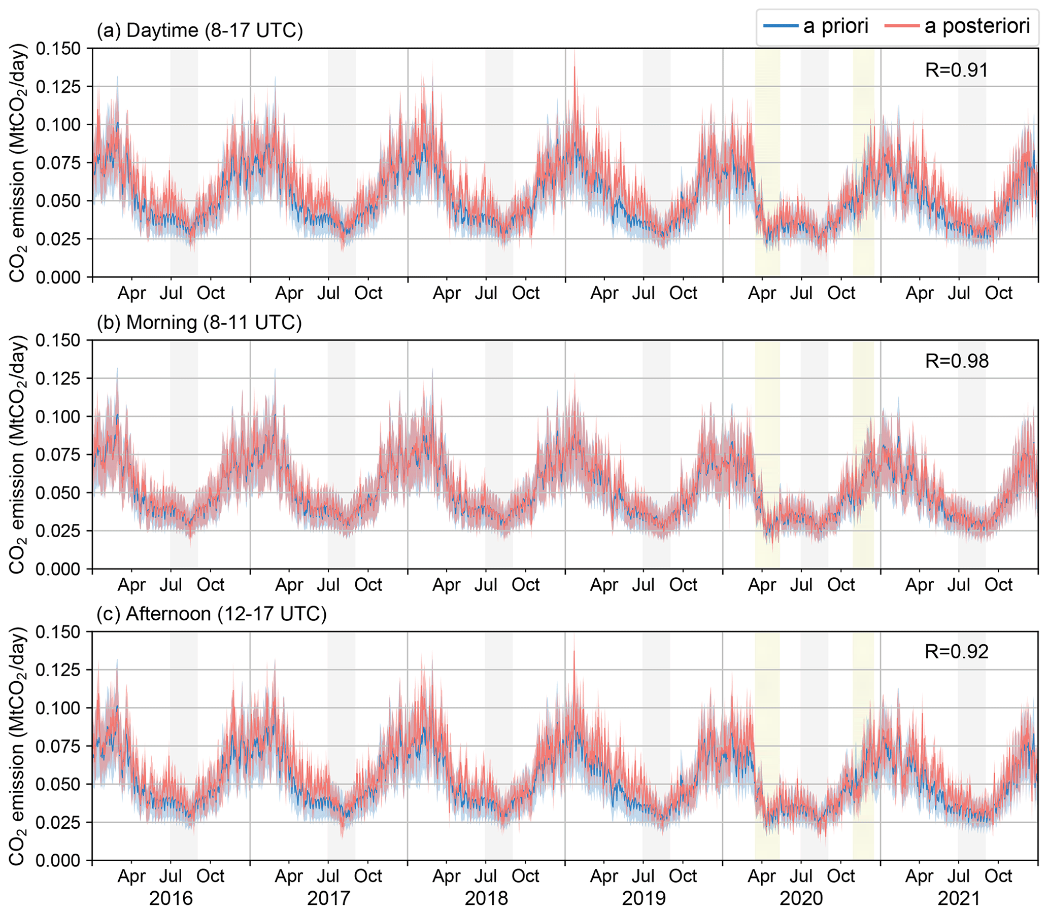
Figure 4 Daily estimates of fossil fuel CO₂ emissions over the greater Paris region when assimilating (a) daytime (08:00–17:00 UTC), (b) morning (08:00–11:00 UTC) and (c) afternoon (12:00–17:00 UTC) CO₂ concentration observations. The blue line and shading show the prior flux according to the Origins.earth inventory together with its assumed uncertainty. The pink and shading show the posterior estimates with their uncertainty ranges. The yellow shaded areas are the two COVID-19 lockdown periods in France. The grey shaded areas are the summer holidays in July and August.

3.2 Monthly emission estimates

Figure 5a shows the posterior estimate of the monthly fossil fuel CO₂ emissions over the greater Paris region derived through a temporal aggregation of the four 6 h period results. Results for the rest of the IdF region are given in Fig. S7. The inversion tends to increase the annual fossil fuel emissions by 2 %–6 % with respect to the prior estimates for every year from 2016 to 2021. It demonstrates the consistency of the measurement constraint on inverse fossil fuel CO₂ emissions over time. It is important to note that the inversions for the years 2016 and 2017 were carried out with the prior emissions from the 2018 Origins.earth inventory, causing the inverse emission changes to mainly rely on the assimilated CO₂ observations. With the same prior emissions for 2017 and 2018, the inversion leads to an emission reduction of 0.6 % over the greater Paris region from 2017 to 2018, which is consistent with the general trend towards a decrease in emission.

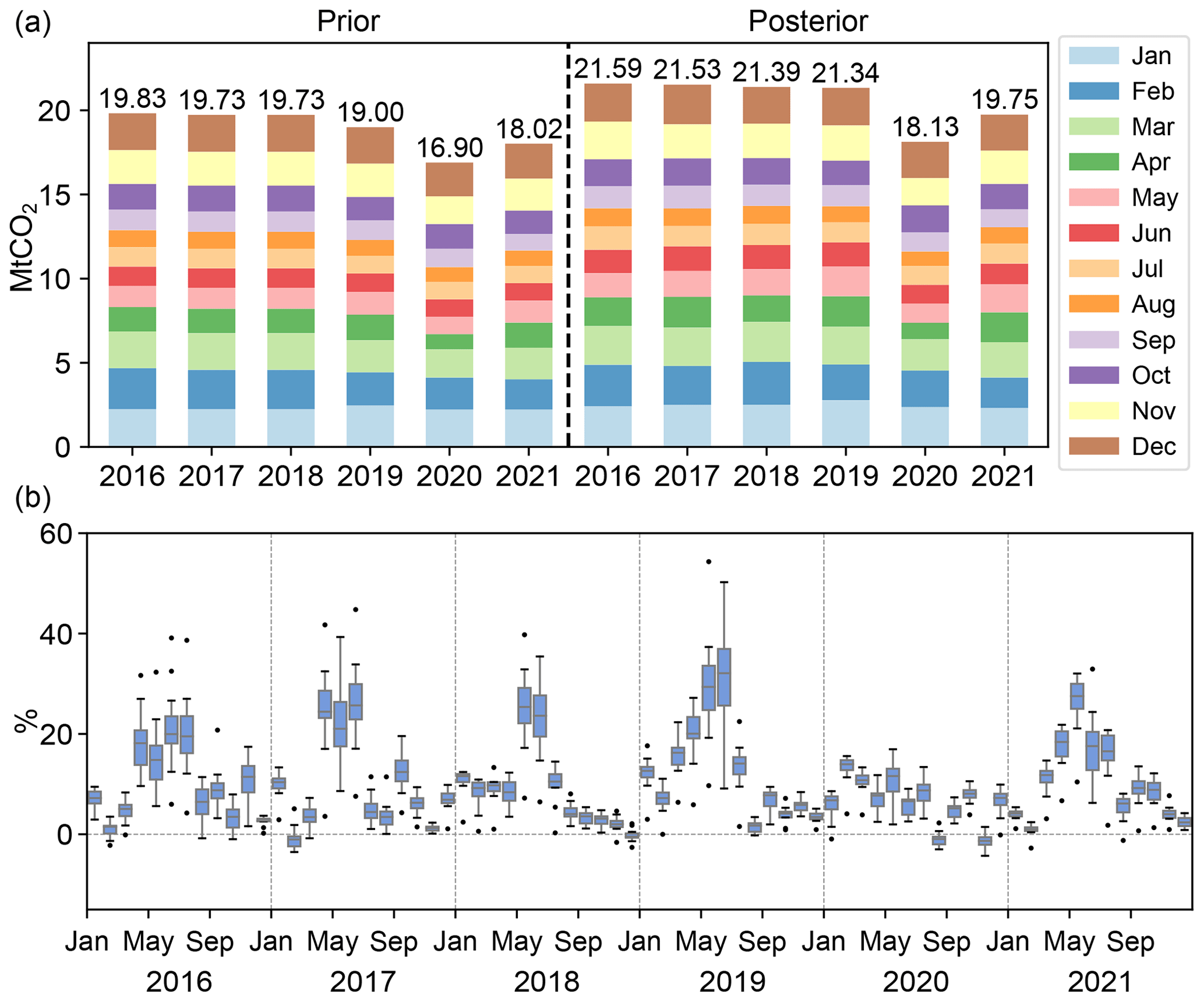
Figure 5 (a) Prior and posterior estimates of the monthly total fossil fuel CO₂ emission over the greater Paris region. (b) The change in CO₂ emissions in percentage $(\text{posterior}-\text{prior})/\text{prior}$. The boxplots are the posterior emissions from an ensemble of sensitivity tests of the inversion configuration. Note that the prior emission for 2016 is slightly higher than for 2017 and 2018 since it is a leap year.

Figure 5b shows the relative difference between the posterior and prior fossil fuel CO₂ emissions corresponding to the different inversion setups (e.g., prior errors and correlation length). It is worth noting that the optimized monthly emissions are very similar across the 6 years from 2016 to 2021. More precisely, the inversion consistently points to an average 10 % increase in fossil fuel emissions in winter months compared with the prior (January to March). Further, the inverse emissions show significantly higher values (>20 %) with respect to the prior during the spring period (especially in May and June). In contrast, minor differences between the prior and posterior estimates are observed for the rest of the year. The ensemble of posterior fluxes, as represented by the spread of the minimum and maximum values among multiple inversions, provides an estimate of the variability introduced by a wide range of inversion setups. Even though these sensitivity tests may not represent the full potential range of uncertainties in the posterior fluxes, they still give us a certain degree of confidence in the inversion results because these variabilities are mostly smaller than the posterior–prior emission differences and the emissions uncertainties.

We then conduct a series of analyses to investigate the potential explanations for the adjustments to the prior fluxes made by the inversion. First, we infer that the seasonal variability in flux adjustments is not caused by biases in the atmospheric transport model. This is because the model–observation misfits in wind speed exhibit a relatively constant pattern throughout a year without a pronounced seasonality (Fig. S8). Second, the 10 % increase in fossil fuel CO₂ emissions during the winter months (January to March) could be due to an underestimation of the residential emissions in the Origins.earth inventory. The temporal profiles of the Origins.earth residential emissions are based on a proxy quantity derived from real-time domestic gas consumption data (Text S3), whereas in reality, this seasonal cycle in the prior emissions may underestimate wintertime energy demands from other fuel types, especially for petroleum and wood burning in the suburban residential areas (Fig. S9). Notably, the estimated monthly emissions are ∼20 % larger compared with the prior estimates from April to June. Part of the adjustments of emissions could be due to an underestimation of the biogenic fluxes from the VPRM model (Text S4). Figure S11 shows an obvious discrepancy between the VPRM-simulated hourly biogenic flux (net ecosystem exchange, NEE) and the eddy flux measurements, especially during the growing season, at the Grignon cropland station located about 40 km west of the center of Paris (Fig. S10). The model–observation comparison of the vertical differences in CO₂ concentrations at the SAC station (15 and 100 m above ground level) shows that the contribution of the nighttime biogenic respiration to the CO₂ concentration could also be a potential source of modeling errors during the growing season (Lian et al., 2021).

3.3 Annual emission estimates

Verifying annual emission totals and tracking emission trends over time using multiple methods constitute an indication of the reliability of inverse emissions estimates. Moreover, given the potential impact of atmospheric transport errors on the emission estimates, and assuming that the model errors do not change statistically over time, the emission trends are expected to be less sensitive to model biases than the emissions estimates. The interannual variations are a critical metric to assess the effectiveness of the CO₂ mitigation efforts. Figure 6 shows the multiyear trend in the annual total fossil fuel CO₂ emissions over the IdF region for the 2005–2021 period. The prior and inverse emissions are compared with multiple inventory datasets. The interannual variation in fossil fuel CO₂ emissions indicates a decreasing trend over the IdF region during the 2005–2021 period using the Mann–Kendall (MK) trend test at a 5 % significance level (p values (0.0001)<0.05). According to the TNO 6 km inventory, this is mainly linked to the emission reductions in the residential and industrial sectors and is further a result of a decrease in coal use, an improvement in energy efficiency and building renovation. The inverse annual fossil fuel CO₂ emissions have been declining at a rate of ∼2 % ± 0.6 % per year over the 6-year period from 2016 to 2021 (MK test p values (0.02)<0.05). In 2020, the COVID-19 pandemic and the continued levels of restrictions in place resulted in a dramatic decline in human activity. Our inversion results indicate a ∼13 % (12 %–14 %) reduction in the annual emissions in 2020 compared with 2019, which is 2 % (1 %–3 %) larger than the prior estimate based on the Origins.earth inventory (11 %). The inverse annual emissions in 2021 rose by about 5.2 % ± 14.2 % to 34.3 ± 2.3 Mt CO₂ compared with 2020 (32.6 ± 2.2 Mt CO₂) but still remained −8.0 % ± 12.6 % compared with the pre-COVID-19 level in 2019 (37.3 ± 2.6 Mt CO₂).

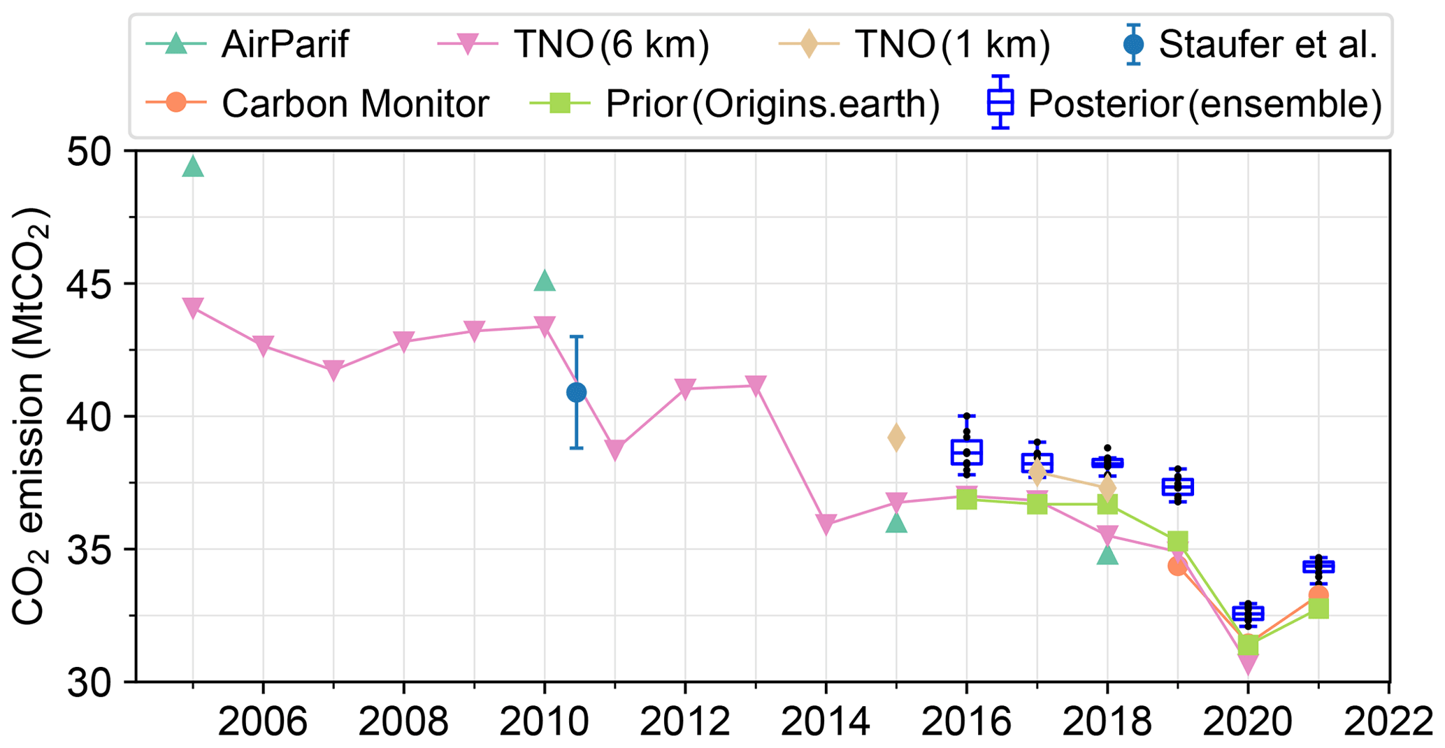
Figure 6 Annual fossil fuel CO₂ emissions over the IdF region from 2005 to 2021. The blue boxplots present the distribution of posterior CO₂ emissions from an ensemble of sensitivity tests of the inversion configuration.

The aggregated annual fossil fuel CO₂ emissions obtained with the inversion are on average higher by ∼5 % for each year compared with the prior estimates from the Origins.earth inventory. Our inversion results are in agreement with the TNO 1 km inventory for all city-scale fossil fuel CO₂ estimates for the years 2017 and 2018, while they are approximately 8.6 %, 3.6 % and 3.1 % higher than those estimated by Carbon Monitor Cities for the years 2019, 2020 and 2021, respectively. In 2018, the optimized emission is 38.1 ± 2.6 Mt CO₂. It is around 3.3, 2.7 and 0.8 Mt CO₂ higher than that from the AirParif, TNO 6 km and TNO 1 km inventories, respectively. Generally, the agreement among the various estimates of the annual fossil fuel CO₂ emissions over the IdF region is within 10 %, demonstrating robust emission estimates at the city scale through a combination of up-to-date inventories, atmospheric modeling and observations. It also provides evidence for a continuous and timely monitoring of urban fossil fuel CO₂ emission trends toward the accomplishment of reduction targets in order to achieve carbon neutrality.

4 Conclusions and discussions

This study shows the capacity of our city-scale inversion system, with a state-of-the-art inventory and high-precision continuous CO₂ measurements, for a timely and an effective monitoring of urban fossil fuel CO₂ emissions over a long time period from 2016 to 2021. Our results indicate a decreasing trend in the annual CO₂ emissions over the IdF region with an amplitude of ∼2 % ± 0.6 % per year at a 5 % significance level. The comparison of both prior and posterior annual emissions with independent estimates from other inventory datasets shows a less than 10 % difference, which is a satisfying target in terms of emission trend detection and verification for Paris in order to support its emissions-mitigation measures and related policy (Wu et al., 2016). In practice, few cities have such a high-resolution near-real-time local inventory like Paris. Through using the same annual total emission as a prior for the years 2016–2018, the posterior emissions exhibit an emission change by about −3 % ± 13.8 % over the IdF region when comparing the year 2016 with 2018. This demonstrates the ability of the inversion system to detect emission changes based on CO₂ measurements, independently of the information provided by the prior inventory. In addition to the afternoon CO₂ measurements that are commonly used in the CO₂ inversion system, the assimilation of morning CO₂ data when the ABL heights are well reproduced by the model could lead to an additional 11 %–16 % uncertainty reduction in the morning fossil fuel emissions. But it is worth pointing out that the selection of morning CO₂ observations only for moderate-to-high wind speeds might reduce the observational constraint on the emissions in stable weather periods.

The uncertainties in the posterior estimates of CO₂ emissions are caused to a certain extent by errors in the spatiotemporal distribution of emissions at scales finer than the targeted ones. The present inversion system mainly controls the city-scale fossil fuel CO₂ emissions but not the finer resolution in space. We thus further conducted a sensitivity inversion test using the TNO 1 km inventory as a priori as an alternative to the Origins.earth dataset for 2018. The other parameters were kept identical to the reference inversion configuration. The TNO inventory indicates more fossil fuel CO₂ emissions concentrated within inner Paris compared with the Origins.earth dataset (Fig. S12). The inversion was able to spatially differentiate between Paris' city center and the greater Paris region (excluding Paris), correcting the respective emissions differently (Fig. S13). The posterior fossil fuel CO₂ emissions from Paris' city center were adjusted more upwardly with Origins.earth than with TNO, while those from the rest of the greater Paris region were corrected at a similar magnitude between Origins.earth and TNO. One can hope that a spatially explicit inversion system would allow us to solve the spatial distribution of urban emissions at the grid scale (Lauvaux et al., 2016). However, this will need additional information in order to determine the spatial correlation length of the inventory uncertainty or a high-density observation network in order to constrain the emissions from a large part of the city (Nalini et al., 2022).

Improvements in urban ecosystem modeling and monitoring for a precise accounting of urban biomass in the estimates of CO₂ fluxes are a relatively recent endeavor. Focusing on the Paris urban area, two limitations of this study are acknowledged and are considered worthy of further investigation. Firstly, due to the coarse-resolution SYNMAP land use (1 km) data (Jung et al., 2006) and the MODIS satellite-derived vegetation indices (500 m) used for the VPRM model, the simulated biogenic fluxes in Paris in this study are almost zero, except for a few grid cells containing two big parks that are located in the eastern and western outskirts of Paris. In reality, there are still a number of green spaces and pervious landscaped areas unevenly distributed in Paris that need to be considered with a fine-scale (sub-kilometer) model. Secondly, there is a lack of detailed evaluation of the Paris VPRM model since no eddy covariance measurement is available within Paris and its surroundings yet. Our analyses indicate that the actual biogenic fluxes within the IdF region may have a recognizable influence on the measured CO₂ concentration gradients, whereas these biosphere signals are not well reproduced by the VPRM model. These discrepancies question the validity of the assumption that the signature of the local biogenic fluxes is not significant compared with that of the fossil fuel emissions in the measured gradients. Even though we have scaled up the prescribed observation errors to account for this possible large model bias in the biogenic fluxes and thereby to reduce its interference in the inverse fossil fuel emissions, the results may inevitably still be hampered. This study highlights the need for an in-depth analysis of the seasonal and daily variations in the biogenic fluxes within the IdF region, especially during the cropland growing season. This could be achieved by improving the default VPRM model with a modified gross primary production and ecosystem respiration equations, domain-specific optimized parameters, high-resolution input datasets, and high-quality diagnostic phenology (Gourdji et al., 2022). In addition, measurements of carbon isotopes (¹⁴C, ¹³C) and tracers co-emitted with CO₂ (e.g., CO, NO_x, VOCs) could also be used to separate the contributions from fossil fuel and biogenic components to the total CO₂ concentrations, which would be beneficial for the optimization of sectoral CO₂ fluxes.