Identifying climate model structural inconsistencies allows for tight constraint of aerosol radiative forcing

Aerosol radiative forcing uncertainty affects estimates of climate sensitivity and limits model skill in terms of making climate projections. Efforts to improve the representations of physical processes in climate models, including extensive comparisons with observations, have not significantly constrained the range of possible aerosol forcing values. A far stronger constraint, in particular for the lower (most-negative) bound, can be achieved using global mean energy balance arguments based on observed changes in historical temperature. Here, we show that structural deficiencies in a climate model, revealed as inconsistencies among observationally constrained cloud properties in the model, limit the effectiveness of observational constraint of the uncertain physical processes. We sample the uncertainty in 37 model parameters related to aerosols, clouds, and radiation in a perturbed parameter ensemble of the UK Earth System Model and evaluate 1 million model variants (different parameter settings from Gaussian process emulators) against satellite-derived observations over several cloudy regions. Our analysis of a very large set of model variants exposes model internal inconsistencies that would not be apparent in a small set of model simulations, of an order that may be evaluated during model-tuning efforts. Incorporating observations associated with these inconsistencies weakens any forcing constraint because they require a wider range of parameter values to accommodate conflicting information. We show that, by neglecting variables associated with these inconsistencies, it is possible to reduce the parametric uncertainty in global mean aerosol forcing by more than 50 %, constraining it to a range (around −1.3 to −0.1 W m⁻²) in close agreement with energy balance constraints. Our estimated aerosol forcing range is the maximum feasible constraint using our structurally imperfect model and the chosen observations. Structural model developments targeted at the identified inconsistencies would enable a larger set of observations to be used for constraint, which would then very likely narrow the uncertainty further and possibly alter the central estimate. Such an approach provides a rigorous pathway to improved model realism and reduced uncertainty that has so far not been achieved through the normal model development approach.

1 Introduction

The most uncertain component of human forcing of the climate system over the industrial period is aerosol effective radiative forcing (ΔF_aer; Forster et al., 2023). Uncertainty in historical ΔF_aer reduces our ability to confidently project near-term future changes to our climate (Andreae et al., 2005; Seinfeld et al., 2016; Peace et al., 2020; Fyfe et al., 2021). The best estimate of ΔF_aer based on the current understanding of aerosols, clouds, radiation, and their interactions (informed by results from global climate models and analysis of observations) ranges from −3.2 to −0.4 W m⁻² (Bellouin et al., 2020). The magnitude of ΔF_aer has remained uncertain through all Intergovernmental Panel on Climate Change assessment reports (Forster et al., 2023) despite decades of research to improve our scientific understanding of the key processes and abundant observations with which to test models.

The lower (most negative) bound of ΔF_aer is more tightly constrained by global mean energy balance arguments, which infer the magnitude indirectly based on historical emissions and changes in global mean surface temperature. Such studies suggest the lower bound may be around −1.8 to −1.7 W m⁻² (e.g. Aldrin et al., 2012; Skeie et al., 2014, 2018). Evidence for a weaker (less negative) lower bound of ΔF_aer comes from energy balance relationships that are additionally informed by output from global climate model ensembles. For example, Smith et al. (2021) constrain the ΔF_aer lower bound to around −1.5 W m⁻², and Albright et al. (2021) constrain the lower bound to between −1.8 and −1.3 W m⁻². However, tight constraint of just the magnitude of historical and future global mean ΔF_aer does not produce a climate model that can be used to explore the full range of regional and global climatic effects. Thus, although energy balance constraints and emergent constraint methods (e.g. Watson-Parris et al., 2020) can set the plausible bounds of the historical global mean ΔF_aer (and/or its components), we also need a process-based approach for building reliable global climate models that can accurately simulate the observed state and behaviour of aerosols, clouds, and radiation that will determine the regional patterns of aerosol effects on future climate (Williams et al., 2022).

A process-based constraint of ΔF_aer is a substantial undertaking, with many steps involved. It relies mainly on using complex climate models to simulate the underlying physical processes that affect changes in aerosols, clouds, and radiation (and hence ΔF_aer) then settling on models that have been developed and refined to achieve acceptable agreement with extensive observations of these atmospheric properties and trends. It is assumed that good agreement of a model simulation with observations ensures that the model is able to make trustworthy estimates of historical ΔF_aer and reliable projections of future ΔF_aer, which cannot themselves be observed. Yet the process-based uncertainty range has remained far wider than estimates from energy balance approaches because models simulate a very large number of complex and regionally varying processes that can affect the magnitude of global mean ΔF_aer (Carslaw et al., 2013; Regayre et al., 2015; Qian et al., 2018; Yoshioka et al., 2019).

A further challenge in process-based constraint is that the range of ΔF_aer stems from two sources of uncertainty in climate models: structural uncertainty and parametric uncertainty. Structural deficiencies in a model are associated with coding choices related to spatial resolution, numerical methods, parameterisation schemes, and neglected processes. Model developments attempt to reduce these deficiencies and the biases they cause compared to observations, and multi-model intercomparisons (Gliß et al., 2021; Thornhill et al., 2021) can be used to estimate a range of ΔF_aer across sets of structurally different models (structural uncertainty). Within a particular model, the uncertain parameters in the process equations cause an additional uncertainty in simulations of ΔF_aer (parametric uncertainty). Adjustment of parameter values, or tuning, is performed during and/or following model development to further improve the goodness of fit to observations (e.g. Hourdin et al., 2017), although it is recognised that well-tuned models still have a large (and usually unquantified) parametric uncertainty (Lee et al., 2016). Perturbed parameter ensembles (PPEs) of the kind we use here (see Sect. 2.1.2) are a substantial extension of normal model tuning; they explore many combinations of parameter values across their likely uncertainty ranges and quantify their combined effects on ΔF_aer (Carslaw et al., 2013; Regayre et al., 2018; Yoshioka et al., 2019). The resulting unconstrained uncertainty in ΔF_aer, from sampling all the important sources of parametric uncertainty in our model, is larger than the range based on energy balance constraints and is approximately as wide as the multi-model range (which conflates structural and parametric uncertainties without fully sampling either), suggesting that parametric uncertainties in ΔF_aer are as important as structural model differences.

Separation of structural and parametric sources of model uncertainty is important because they have different remedies. Structural uncertainties point to model deficiencies that require model developments, while parametric uncertainties can be reduced by matching the outputs of many model variants (parameter combinations) to historical observations through a process called history matching (Craig et al., 1997a; Williamson et al., 2013; Vernon et al., 2014; Johnson et al., 2020; Regayre et al., 2020). There is currently no best practice for accounting for and separating the effects of structural and parametric uncertainties (Sexton et al., 2012; Brynjarsdóttir and O'Hagan, 2014; McNeall et al., 2016; Johnson et al., 2020; Rostron et al., 2020). In particular, the observational constraint of parametric uncertainty cannot be cleanly separated from the effects of structural uncertainties. For example, without accounting for potential (usually unquantified) structural errors, it may not be possible to find any parameter combinations that produce a model that is consistent with all target observations. Therefore, it is common to add a structural error term during model–observation comparison (e.g. Sexton et al., 2012), which effectively inflates the parametric uncertainty and the overall model uncertainty to accommodate the structural errors. This approach avoids overfitting and provides an estimate of the uncertainty in ΔF_aer that broadly accounts for both sources of uncertainty. However, it does not provide any information about which processes cause structural model errors nor how they weaken the constraint of parameter values and the range of ΔF_aer.

To maximise ΔF_aer constraint, we need to address three key challenges. First, we need to densely sample the model parametric uncertainty related to the multitude of cloud, aerosol, and physical atmosphere processes that determine ΔF_aer. Secondly, we need to identify model variables that share causes of uncertainty with ΔF_aer to prioritise associated observations for use in the constraint process (Carslaw et al., 2013; Regayre et al., 2020). The final challenge is to ensure that any constraint on ΔF_aer is consistent across multiple observation types and/or to quantify the limiting effect of any internal model inconsistencies on ΔF_aer constraint. Here, we tackle these challenges using 1 million variants of version 1 of the UK Earth System Model (UKESM1; Sellar et al., 2019) (based on statistical emulators trained on outputs from 221 model simulations) that sample ΔF_aer uncertainty (Sect. 3.1) caused by 37 aerosol, cloud, and physical atmosphere model parameters (Table S1 in the Supplement). We evaluate the causes of uncertainty in cloud properties over stratocumulus-dominated regions (Sect. 3.2) and observationally constrain ΔF_aer using tens of thousands of combinations of more than 450 satellite-derived values (Sect. 3.3). This approach exposes previously hidden structural inconsistencies related to representations of cloud properties in the model. We remove variables associated with these inconsistencies from the constraint process to produce an internally consistent constraint on ΔF_aer. This constraint does not make use of all available observations; therefore, our central estimate of forcing may not be the final best value, which would ultimately be achieved in a model with no remaining structural deficiencies. However, we argue that, in a model with fewer structural inconsistencies, our approach could constrain ΔF_aer and associated process uncertainties even further.

2 Methods

Our approach is summarised in Fig. 1.

Figure 1 Flow chart detailing the procedure to densely sample model parameter uncertainty, evaluate model variants against observations, identify potential structural inconsistencies, and constrain ΔF_aer.

2.1 Experimental design

2.1.1 Model version

We used the atmosphere-only configuration of version 1 of the UK Earth System Model (UKESM1; Sellar et al., 2019) to create our PPEs (Sect. 2.1.2). UKESM1 was the model version submitted to the 6th Coupled Model Intercomparison Project (CMIP6; Eyring et al., 2016). UKESM1 is based on the HADGEM3-GC3.1 physical climate model (Williams et al.,  2018) with additional coupling to key Earth system processes (Sellar et al., 2019), including the United Kingdom Chemistry and Aerosol (UKCA) model (Archibald et al., 2020). The atmosphere-only configuration used here consists of the GA7.1 atmosphere (Walters et al., 2019; Mulcahy et al., 2020), with additional aerosol, cloud, and physical atmosphere structural updates as implemented in UKESM1 (Mulcahy et al., 2020). GA7.1 includes several structural advancements to the aerosol component of the model which significantly affect anthropogenic aerosol radiative forcing (Mulcahy et al., 2018). We refer to this model version as UKESM1-A.

We use an N96 horizontal resolution, which is 1.875^∘ × 1.25^∘ (208 km × 139 km) at the Equator, with 85 vertical levels between the surface and 85 km in altitude. Model vertical levels use a stretched grid such that the vertical resolution is around 13 m near the surface and around 150 to 200 m at the top of the boundary layer. We chose this resolution since it is the same as that used for long climate runs in CMIP6.

Horizontal wind fields above around 2 km in our simulations (model vertical level 17) were nudged towards ERA-Interim values for the period December 2016 to November 2017. Nudging is intended to remove the effects of differences in large-scale meteorology between our PPE members, meaning we can attribute differences between model variants to perturbed parameter values. We do not nudge winds within the boundary layer as many of our parameters are intended to affect meteorological conditions, in particular cloud adjustments, in this part of the atmosphere.

The model was forced using anthropogenic SO₂ emissions for the years 2014 and 1850, as prescribed in CMIP6 simulations. We separately calculated components of ΔF_aer (Forster et al., 2023) caused by aerosol–cloud interactions (ΔF_aci) and aerosol–radiation interactions (ΔF_ari) using differences in top-of-the-atmosphere radiative fluxes between these two periods. The separation of these ΔF_aer components accounts for above-cloud aerosol radiative effects (Ghan et al., 2016) and multiple cloud adjustments (Grosvenor and Carslaw, 2020).

Carbonaceous aerosols from fossil fuel and residential sources match those used in CMIP6 in our early-industrial simulations. However, in our present-day simulations, we prescribed carbonaceous aerosol from biomass burning sources using emissions generated using Copernicus Atmospheric Monitoring Service (CAMS) Information for December 2016 to November 2017 (CAMS: Global biomass burning emissions based on fire radiative power (GFAS): data documentation) and spread these emissions between the surface and around 3 km. We used emissions for the same period as prescribed wind fields for the closest possible comparison to observed values. In our early-industrial simulations (1850 anthropogenic SO₂ emissions) we similarly spread CMIP6 carbonaceous aerosol from biomass burning over model levels between the surface and around 3 km.

We also prescribed rather than simulated sea surface temperatures and sea ice fraction to best match the December 2016 to November 2017 period. We prescribed land surface quantities, ocean surface concentrations of dimethylsulfide (DMS) and chlorophyll, and atmospheric concentrations of gas species (including oxidants OH and O₃, which we then perturb) using monthly mean output values from a fully coupled version of the UKESM model, averaged over the 1979 to 2014 period. Additionally, we prescribe volcanic SO₂ emissions for continuously emitting and sporadically erupting volcanoes (Andres and Kasgnoc, 1998) and for explosive volcanic eruptions (Halmer et al., 2002).

Aerosol number concentrations are treated prognostically with the GLOMAP multi-modal scheme (Mann et al., 2010, 2012), which uses five log-normal aerosol size modes and includes sulfate, sea salt, black carbon, and organic carbon chemical components that are internally mixed within each size mode. Mineral dust is simulated separately using the CLASSIC dust scheme (Woodward, 2001). GLOMAP simulates new particle formation, coagulation, gas-to-particle transfer, cloud processing, and deposition of gases and aerosols. The activation of aerosols into cloud droplets is calculated using distributions of sub-grid vertical velocities based on available turbulent kinetic energy (West et al., 2014), and the removal of cloud water by autoconversion to rain is calculated by the host model using a single-moment cloud microphysics scheme. Aerosols are also removed by impaction scavenging of falling raindrops according to the collocation of clouds and precipitation (Lebsock et al., 2013; Boutle et al., 2014).

We modified some aspects of UKESM1-A and perturbed key parameters related to these uncertain processes in the PPE. Including these structural changes adds complexity to our model, which we consider to be worthwhile given their potential to interact with other processes and affect ΔF_aer. Firstly, we defined an ice mass fraction threshold (cloud_ice_thresh; Table S1) above which no nucleation scavenging occurs to allow sufficient aerosol to be transported to the Arctic (Browse et al., 2012). We assumed that the wet scavenging of all aerosol particles (soluble and insoluble) is zero in large-scale raining clouds if the simulated ice-to-total-water mass fraction is higher than this fixed value. This first structural change replicated the model change we implemented in Yoshioka et al. (2019), which is not yet in the released version of the model. We evaluated the climatic importance of this parameter as a cause of ΔF_aer uncertainty in Regayre et al. (2018, 2020), Johnson et al. (2020), and Peace et al. (2020). Secondly, we implemented a version of look-up tables for aerosol optical properties (Bellouin et al., 2013) that includes optical properties for mineral dust (Balkanski et al., 2007) and higher-resolution increments of the imaginary part of the refractive indices to better resolve the absorption coefficient of aerosols. Finally, we included an organically mediated boundary layer aerosol nucleation parameterisation (Metzger et al., 2010) to enhance remote marine and early-industrial aerosol concentrations in the model.

2.1.2 Perturbed parameter ensembles

We created a new PPE of 221 model simulations for this study. Each member of the PPE has a distinct combination of 37 aerosol and physical atmosphere parameter values (Table S1). Parameters perturbed in previous PPEs using older versions of the model (Yoshioka et al., 2019; Sexton et al., 2021) and identified as important causes of uncertainty in cloud active aerosol concentrations and/or aerosol forcing (Carslaw et al., 2013; Regayre et al., 2015, 2018) were perturbed here alongside parameters associated with structural model developments (Mulcahy et al., 2018, 2020; Walters et al., 2019). Following Regayre et al. (2015), Yoshioka et al. (2019), and Sexton et al. (2021), uncertain parameter ranges were determined by formal expert elicitation using the approach described in Gosling (2018).

We created the PPE in two stages following history-matching conventions (Craig et al., 1997b; Williamson et al., 2013). The main benefit of a multi-stage observational constraint is that it maximises computational efficiency and the value of information in the final-stage PPE by ruling out the most implausible parts of parameter space in earlier stages. We describe both stages here. However, the second-stage PPE is the focus of our analysis. The PPEs in both stages have a ratio of simulations to uncertain parameters of around 6 to ensure that the ensembles accurately represent model responses across the 37-dimensional parameter space.

In the first stage, the 221-member ensemble was made by combining a simulation using median values for each parameter with 220 additional parameter combinations drawn from a Latin hypercube optimised to ensure that design points were distributed as evenly as possible across the parameter space using the optimumLHS R function (Stocki, 2005). To extend the sample of model simulations from 221 to 1 million model variants, we created statistical Gaussian process emulators (O'Hagan, 2006) that densely sampled model parameter uncertainty. We evaluated a single month of model output (May 2015 to match nudged wind fields for this stage) and ruled out model variants (parameter combinations) that compared poorly to global and regional mean observations. At this stage, observations included global mean shortwave and longwave top-of-the-atmosphere radiative fluxes from the Clouds and the Earth's Radiant Energy System (CERES SYN1deg Ed4A obtained from the NASA Langley Research Center CERES ordering tool at https://ceres.larc.nasa.gov.data/; last access: 1 August 2023) experiment and global mean precipitation amount from version 2 of the Global Precipitation Climatology Project (GCPC; Adler et al., 2003; provided by NOAA PSL, Boulder, Colorado, USA, from their website https://psl.noaa.gov, last access: 1 August 2023). Additionally, we used North Pacific and North Atlantic marine-only data between 10 and 60^∘ N for low- and total-cloud fraction from the Moderate Resolution Imaging Spectroradiometer (MODIS) and liquid water path (LWP) from the Multi-Sensor Advanced Climatology of Liquid Water Path data set (available at the Goddard Earth Sciences Data and Information Services Center, https://disc.gsfc.nasa.gov, last access: 3 August 2023). We assumed model–measurement comparison errors of 8 %, 2 %, 30 %, 20 %, 20 %, and 40 % respectively for these observations.

For the second (final) stage, we identified the model variant closest to the centre of the not-ruled-out parameter space then iteratively identified 220 additional parameter combinations with the greatest Euclidean distance from existing points until we had a new and diverse set of 221 members that spanned the uncertain parameter space retained from the first stage. Thus, second-stage PPE members correspond to a diverse set of parameter combinations from the not-ruled-out-yet set of first-stage model variants. As in the first stage, we created and validated (e.g. Fig. S1 in the Supplement) statistical emulators of global mean and regional mean variables and used these emulators to extend the output from 221 simulations to 1 million model variants.

2.2 Measurements

We evaluated the potential of several types of observations related to clouds and aerosol–cloud interactions in multiple locations and at multiple times of the year to serve as global mean ΔF_aer constraints, and we refer to them collectively as “constraint” variables.

2.2.1 Regional mean cloud and radiative properties

We compared physical and radiative properties of clouds derived from MODIS instruments (King et al., 2003) to model outputs calculated using the Cloud Feedback Model Intercomparison MODIS satellite simulator (Bodas-Salcedo et al., 2011; Saponaro et al., 2020) where available. This simulator minimises errors in model comparisons to MODIS retrieval data by recreating as nearly as possible what the satellite would retrieve given model-simulated atmospheric conditions.

We used MODIS retrievals of LWP, liquid cloud fraction (f_c), cloud optical depth (τ_c), and cloud droplet effective radius (r_e) at 1^∘ × 1^∘ resolution and used τ_c and r_e values to calculate cloud droplet number concentration (N_d). We assumed constant N_d throughout cloud layers, which is a good approximation for stratocumulus clouds (Grosvenor and Carslaw, 2020; Painemal and Zuidema, 2011), and compared observed N_d to values calculated at model-simulated cloud tops. Additionally, we used outgoing top-of-the-atmosphere shortwave radiative flux (F_SW) measurements (SYN1deg Ed4A, obtained from the NASA Langley Research Center CERES ordering tool at https://ceres.larc.nasa.gov/data/, last access: 1 August 2023).

All satellite-derived measurements were degraded to match the model resolution, then averaged over time and space for each region. We then identified regions with high cloud fraction across the year (Table S2). We evaluated constraint variables at the regional level since there are no clear relationships between aerosol forcing and observations of global mean values (Fig. S2). The chosen regions are dominated by stratocumulus cloud, have relatively high multi-model diversity in terms of cloud amount in CMIP6 models (Vignesh et al., 2020), and are the most important regions for understanding the role of aerosol–cloud interactions (Langton et al., 2021). We only used values corresponding to model grid boxes with at least 50 % ocean coverage in our area-weighted regional mean calculations.

These constraint variables are defined as monthly mean, annual mean, or seasonal amplitude (difference between maximum and minimum monthly mean values) within each region. So, for each of our six observation types (F_SW, N_d, f_c, LWP, τ_c, and r_e), we have 70 constraint variables (12 months, annual mean, and seasonal amplitude, all over five regions) for a total of 420 regional cloud and radiative flux constraint variables.

2.2.2 Hemispheric difference in N_d

The contrast between marine N_d in the polluted Northern Hemisphere and the relatively pristine Southern Hemisphere (H_d) can act as a proxy for the difference in N_d between the early-industrial and present-day atmospheres (McCoy et al., 2020). We calculated H_d as the difference in hemispheric mean marine N_d values using MODIS τ_c and r_e values and evaluated 14 constraint variables calculated as annual and monthly means and the seasonal amplitude.

2.2.3 Transects from stratocumulus- to cumulus-dominated regions

Cloud physical and radiative properties are sensitive to changes in aerosol concentrations in regions where stratocumulus clouds transition into cumulus (Christensen et al., 2020, 2022). We identified transects from stratocumulus to cumulus cloud (Fig. S3, Table S3) and evaluated changes in aerosol and cloud along these transects (July or November for the Northern Hemisphere and the Southern Hemisphere respectively) as constraint variables. We refer to these collectively as transect variables. These transect variables include changes in N_d, r_e, f_c, LWP, and aerosol index (AI; the total MODIS aerosol optical depth at 550 nm multiplied by the Ångström exponent) along the transects. Additionally, we included ratios of N_d to AI, r_e to N_d, LWP to N_d, and f_c to N_d along each transect as constraint variables. All transect variables were calculated as gradients of linear relationships between the variable (or ratio of logarithms following McComiskey et al., 2009) and distance (in metres).

Meteorological covariability (changes induced in both variables by shared meteorological drivers) means that these transect variables cannot be used to directly infer the strength of the aerosol effect on clouds (Gryspeerdt et al., 2016), but this is not what we do here. Rather, in order to constrain ΔF_aer, it is only required that the transect variables (calculated identically from the observations and model) share causes of uncertainty and parameter dependencies with uncertain parameters in the model (see Sect. 2.3). In total, we evaluated 36 transect variables calculated using four transects from stratocumulus- to cumulus-dominated regions.

2.3 Relative importance of parameters

One way to prioritise which observations to use for constraint is to quantify the overlap in causes of uncertainty between ΔF_aer and model variables associated with the observations (e.g. Regayre et al., 2020). Variance-based sensitivity analyses (Lee et al., 2012) can be used to robustly quantify the percentage of variance caused by each parameter. However, the multi-stage design of the present PPE (Sect. 2.1.2) potentially leaves gaps in the parameter space that may limit the interpretability of variance-based methods. Therefore, we approximated the relative importance of parameters as causes of uncertainty using Pearson partial correlations (Kim, 2015). Partial correlations control for the effects of all other perturbed parameters on the variable of interest in the calculation of correlations. A partial correlation between a constraint variable and a parameter is the correlation between the residuals from (a) linear regression of the variable on the remaining 36 parameters and (b) linear regression of the parameter on the remaining 36 parameters. For each of the 37 model parameters, we defined the relative-importance metric as the proportion of its partial correlation with the variable to the total of the 37 partial correlations, multiplied by the sign of the gradient of the linear regression of the variable on the parameter in question. We included the sign of the gradient to define whether increasing the parameter value increases or decreases the output variable, which helps to develop a process-based understanding. Relative-importance metrics are used in Sect. 3.2 to guide our choice of variables for model constraint and to inform our understanding of how they relate to ΔF_aer. The metrics were calculated using 1 million model variants (from emulators) for ΔF_aer and its components ΔF_aci and ΔF_ari and using the 221 PPE members for other variables.

2.4 Constraint process

2.4.1 Observationally plausible model variants

In our previous effort to constrain ΔF_aer, we calculated “implausibility” metrics that quantify the implausibility of each model variant for all observed values, accounting for emulator uncertainty, observational uncertainty, interannual variability, and representation errors (Johnson et al., 2020; Regayre et al., 2020). Implausibility metrics were calculated for 1 million model variants across more than 9000 distinct measurements, and we used these implausibility values to rule out model variants as observationally implausible if they did not compare well to the full set of observations. In practice, observations associated with relatively large uncertainties had little to no impact on ruling out model variants. Using this approach, we constrained ΔF_aer and the parameter space but could not readily isolate the role of individual constraint variables on the resulting ΔF_aer constraint and could not quantify how the constraint improved model skill; we could only quantify how it reduced the ΔF_aer uncertainty range.

We did not include (largely unquantified) observational errors in our constraint here because we compare satellite data to model output from satellite simulators, which significantly reduces the importance of this source of uncertainty in observation-to-model comparisons. We also neglected the effects of representation errors (Schutgens et al., 2017) because they are unquantified for the satellite-derived observations used here. Instead, we restricted our model–measurement comparisons to monthly mean values within stratocumulus-dominated regions to reduce the magnitude of these errors. Neglecting observational and representation errors risks over-constraining the model. To avoid over-constraint, we retained a proportion of model variants (at least 5000 or 0.5 %) of the same order of magnitude as earlier constraint efforts that used constraint variables with more readily quantifiable sources of model–observation comparison uncertainty (Johnson et al., 2020; Regayre et al., 2020). In this way, our method avoids over-constraining the model yet allows us to identify potential model structural inconsistencies.

2.4.2 Model–observation differences

We calculated absolute differences between observed and simulated values for each of the 1 million model variants and for each of the 450 constraint variables. For each constraint variable, we then normalised the 1 million absolute difference values and ranked model variants according to their normalised absolute difference (NAD) values to identify which model variants to rule out as least skilful. To further avoid over-constraint, we set the NAD to zero where the uncertainty in the emulators was large relative to the difference between observed and emulated values. In this way, individual constraints are stronger for constraint variables where parameter perturbations clearly define the response surface of the associated statistical emulators. For this step, we defined the emulator uncertainty as the square root of the emulator variance for that specific combination of model parameters. Thus, for each constraint, we retained the larger of either (a) all model variants with errors smaller than the emulator uncertainty or (b) the 5000 model variants with the lowest NAD. For combinations of constraint variables, we calculated the average NAD across all variables for each model variant prior to ranking and rejecting model variants with the highest average NAD across variables.

2.4.3 Identifying viable constraint variables

Constraint variables where the emulator uncertainty (average emulator standard deviation) was larger than the changes in the emulated response surface (standard deviation of emulated values) were considered to have low emulator skill and thus were removed from our analysis. This was the case for a small number of transect constraint variables and for the seasonal amplitude of f_c in the Southern Ocean. Additionally, we removed transect measurements from the set of constraint variables where the observed values were outside the 90 % credible interval of corresponding values in the sample since such discrepancies are indicative of structural model inadequacies and/or unaccounted for observational errors (Figs. S4–S7). In total, we evaluated 1 million model variants against the remaining 450 constraint variables.

2.4.4 Internally consistent constraint variables

We identify a subset of the 450 constraint variables that are “pairwise consistent” with N_d in each region. We defined a variable as being consistent with N_d when the constraint to match N_d did not increase the mean NAD calculated across the remaining model variants in the associated region and vice versa. We used individual monthly mean N_d values (September, October, December, and March and the annual mean for the North Atlantic, North Pacific, South Atlantic, South Pacific, and Southern oceans respectively) to identify which constraint variables could be considered to be regionally pairwise consistent. These months were chosen based on the degree of between-month N_d consistency in each region (see Sect. 3.3.2 and Figs. S8–S11). We assumed constraint variables that are consistent with N_d in these specific months in these regions are also consistent with N_d (and other selected constraint variables) in other regions. Our strategy here is to rule out constraint variables that are clearly inconsistent rather than to ensure internal consistency between all remaining constraint variables. Across all regions, 225 constraint variables were identified as being pairwise consistent with N_d.

2.4.5 An optimal set of constraint variables

An “optimal” set of constraint variables was identified (using our specified set of observations and ensemble of model variants) by first identifying the individual constraint variable (from the 225-member N_d-consistent set) with the greatest impact on ΔF_aci uncertainty (our target model variable) then progressively adding constraint variables that most improved the overall constraint (quantified as a reduction in the 90 % credible interval). That is, we identified the most effective constraint variable, then quantified the constraint efficacy of the remaining 224 variables in combination with the first, and repeated this until ΔF_aci could not be constrained further. To avoid confusing a local maximum constraint with an optimal constraint, we continued to add constraint variables to the optimal set, progressively including constraint variables that weakened the ΔF_aci constraint the least. At each of the more than 20 000 steps in this process, we evaluated the average NAD values for each of the 1 million model variants for every possible additional constraint.

We tested how the order of introducing constraint variables affects the results since a stronger constraint may be achieved using a different set of “optimal” constraint variables. We could not feasibly calculate NAD values for 1 million model variants across all possible combinations of 225 N_d-consistent constraint variables. Instead, we tested the effect of starting with all 225 consistent constraint variables and progressively removing one variable at a time. This is the most distinct test of reordering the constraint variables. This approach yielded a similar “optimal” constraint on ΔF_aer as that achieved by progressively adding constraint variables (see Sect. 3.3.2) and very similar constraints on marginal parameter distributions (see Sect. 3.3.3 and Figs. S12 and S13). Additionally, we tested the impact of our choice to retain 5000 model variants at each step in the constraint process. The number of model variants retained affects the number of constraint variables needed to optimally constrain ΔF_aer, but not in a consistent manner (Fig. S14 and Table S4), since changing the efficacy of individual and combined constraint variables affects the potential for additional observations to further reduce the ΔF_aci uncertainty. However, the strength of constraint and the bounds of constrained ΔF_aer (to one decimal place) are insensitive to the number of model variants retained (Fig. S14 and Table S4).

3 Results

3.1 Sampling uncertainty in ΔF_aer

Industrial-period ΔF_aer ranges from around −3.5 to 3.0 W m⁻² in our set of 1 million UKESM1-A model variants, with a 90 % credible interval of −1.8 to 0.9 W m⁻² (Fig. 2). This unconstrained 90 % credible range (2.7 W m⁻²) is as wide as the credible range (2.8 W m⁻²) based on an in-depth review of evidence from models and observations related to aerosol–cloud and aerosol–radiation interactions (Bellouin et al., 2020) and therefore spans a wide spectrum of model behaviour. The range includes positive ΔF_aer values that stem from positive forcing contributions from ΔF_aci and ΔF_ari (Fig. S15), which the Bellouin review discounts (Bellouin et al., 2020). These positive ΔF_aci and ΔF_ari values arise from individually plausible parameter values that produce seemingly implausible model outputs when combined. As shown below, the associated model variants are amongst those ruled out as observationally implausible after optimal constraint (Sect. 2.4.5).

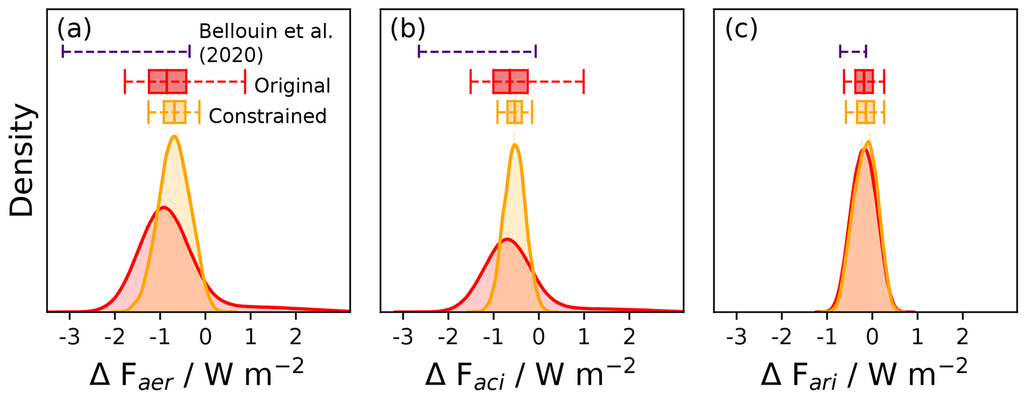
Figure 2 Probability density functions for global, annual mean effective radiative forcings from 1850 to 2014. (a) ΔF_aer, (b) ΔF_aci, and (c) ΔF_ari in the original 1-million-member sample and after optimal constraint (see Sect. 3.3.2). Box plots show the 5th, 25th, 50th, 75th, and 95th percentiles. The 5th and 95th percentiles from Bellouin et al. (2020) are also shown.

3.2 Shared causes of uncertainty and the potential for observational constraint

Our aim is to constrain ΔF_aer as tightly as possible using a set of observations that constrain all processes and associated model parameters that cause ΔF_aer uncertainty. Figure 3 shows that global mean ΔF_aer is sensitive to around 10 model parameters (see Sect. 2.3 and Table S1). Here, we prioritise the constraint of global mean ΔF_aer because it is the quantity most commonly used to inform policy decisions (Forster et al., 2023). We are particularly motivated to constrain processes that cause uncertainty in ΔF_aci since it is the larger and more uncertain component of ΔF_aer (Fig. 2), and the ΔF_ari component can be more readily constrained using available aerosol observations (Johnson et al., 2020; Watson-Parris et al., 2020). Thus, we seek model variables that share causes of uncertainty with global mean ΔF_aer and ΔF_aci. Sharing causes of uncertainty (or parameter sensitivity) with ΔF_aer is a necessary, but not sufficient, condition for constraint (Lee et al., 2016). Model variables and ΔF_aer must also share parameter dependencies (responses to high-dimensional parameter combinations). It is highly unlikely that any one model variable will share exactly the same set of dependencies on uncertain model parameters with ΔF_aer and ΔF_aci (Lee et al., 2016; Regayre et al., 2020). Thus, to constrain model uncertainty, we anticipate needing multiple observations that share at least some causes of uncertainty and parameter dependencies with ΔF_aer and ΔF_aci.

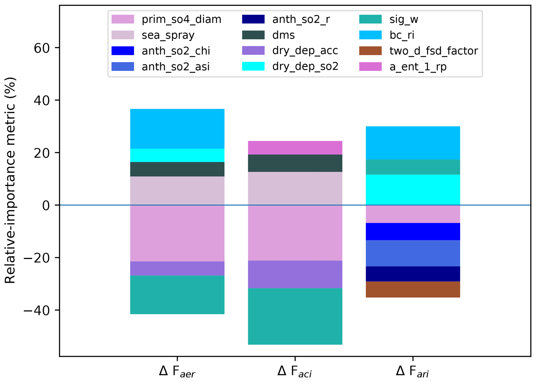
Figure 3 Relative importance of model parameters as causes of uncertainty in global mean ΔF_aer and its components ΔF_aci and ΔF_ari. Only parameters with a relative importance of 5 % or larger are shown. Positive values correspond to parameters where increasing the parameter value causes median values of ΔF_aer, ΔF_aci, or ΔF_ari to become weaker (less negative) across the set of 1 million model variants.

To find a set of useful constraint variables (i.e. a set that collectively shares causes of uncertainty and parameter dependencies with ΔF_aer), we evaluate a diverse set of constraint variables. Causes of uncertainty and the dependence of forcing on these causes are likely to vary regionally and seasonally (Regayre et al., 2015), so observations of the same type over multiple regions and months may all inform the constraint but with some redundancy where sensitivities and dependencies are similar. In total, we have more than 450 constraint variables (see Sect. 2.2) spanning monthly mean, annual mean, and seasonal amplitudes for the global mean H_d and six observation types (F_SW, N_d, f_c, LWP, τ_c, and r_e) across five stratocumulus-dominated regions (state variables) along with nine constraint variables for changes in aerosol and cloud properties and their relationships, each along four transects from stratocumulus- to cumulus-dominated regions (transect variables).

First, we evaluate the causes of uncertainty in ΔF_aer and its components (Fig. 3). There is substantial overlap between the parametric causes of uncertainty in ΔF_aer and ΔF_aci, with the parameter that controls the diameter of newly formed accumulation mode sulfate particles (prim_so4_diam) causing the largest amount of uncertainty. Increasing the value of this parameter increases the diameter of newly emitted sulfate particles and thus decreases the number of particles emitted (for fixed emission mass flux), which makes ΔF_aci more negative (stronger) on average since larger particles are more likely to act as cloud condensation nuclei. Any constraint that rules out the most positive ΔF_aci values will likely constrain newly formed sulfate particles towards higher diameters.

Other key causes of ΔF_aer uncertainty include the parameters controlling sub-grid updraft velocities (sig_w), emission fluxes of sea spray aerosol (sea_spray) and dimethyl sulfide (dms), the dry deposition removal rate of accumulation mode aerosol (dry_dep_acc), and the refractive index controlling carbonaceous aerosol radiative properties (bc_ri). The physical atmosphere parameter controlling cloud top entrainment (a_ent_1_rp) affects ΔF_aci uncertainty, and the parameter controlling sub-grid cloud heterogeneity (two_d_fsd_factor) affects ΔF_ari. However, in contrast with previous PPE analyses of this kind (Regayre et al., 2018; Yoshioka et al., 2019), no physical atmosphere parameters feed through to causes of global mean ΔF_aer, likely due to model structural developments related to clouds and radiation (Walters et al., 2019; Williams et al., 2018).

We understand how the key causes of uncertainty affect ΔF_aci in the model. Increasing the value of the updraft parameter increases N_d, particularly in the present-day atmosphere with relatively high cloud condensation nuclei concentrations, where droplet activation is limited by vertical velocity. Thus, increasing the value of the updraft parameter makes median ΔF_aci more negative (stronger) by increasing cloud albedo, particularly in the relatively polluted present-day atmosphere. The influence of natural emission flux parameters on ΔF_aci uncertainty is well established (Carslaw et al., 2013). Increasing sea spray or dimethyl sulfide emission fluxes makes global mean ΔF_aci less negative (weaker) on average by increasing the background aerosol concentration and thus reducing the sensitivity of cloud albedo to anthropogenic aerosol. The removal rate of accumulation mode aerosol similarly affects background aerosol concentrations. These three parameters also influence present-day N_d in relatively low anthropogenic aerosol environments such as the Southern Ocean (Hamilton et al., 2014), so they can be collectively constrained using appropriate observations (Regayre et al., 2020). However, compensating errors in aerosol emission fluxes and removal rates moderate our ability to constrain these parameters individually (Regayre et al., 2020).

The constraint variable that shares most causes of uncertainty with ΔF_aer and ΔF_aci is H_d, the hemispheric difference in marine N_d. The key parameters that cause uncertainty in ΔF_aci (related to vertical velocities and sea spray emissions) also cause most of the uncertainty in H_d in all months (Figs. 3 and S16). This suggests that we may extract much of the potential constraint from this type of observation using a single representative month (with dependencies on key parameters most closely aligned to ΔF_aci parameter dependencies). Other important parameters (newly formed sulfate diameters, DMS emissions, and dry deposition velocities) also cause H_d uncertainty in some months. Seasonal differences in causes of H_d uncertainty can be traced to regional causes of N_d uncertainty (not shown), so based on shared causes of uncertainty, both H_d and regional N_d observations have potential to constrain ΔF_aci.

Several other observable state variables share key causes of uncertainty with ΔF_aci (Figs. S17–S22). Vertical velocities cause uncertainty in r_e and τ_c (around 20 % to 30 %), as do dry deposition velocities and, to a lesser extent, newly formed sulfate diameters (around 5 % to 10 %). Some transect variables also share causes of uncertainty with ΔF_aci (Figs. S23–26). For example, along the North Atlantic transect, the diameter of newly formed sulfate particles causes up to 50 % of the uncertainty in many transect variables, including variables associated with the cloud albedo response (gradient of the relationship between r_e and N_d for given LWP) and cloud adjustments (LWP and f_c vs. N_d). Vertical velocities cause up to 35 % of the uncertainty in these cloud-related variables in the South Atlantic, whilst dry deposition causes up to 30 % in the South Pacific. These regionally distinct causes of uncertainty suggest that observations from transects in several regions may constrain the model when combined, even if each transect variable constrains just one source of parametric uncertainty. Additionally, the radiative properties of carbonaceous aerosol (an important cause of ΔF_ari uncertainty) causes around 20 % of the uncertainty in several variables along transects in the North Pacific. Thus, North Pacific transect variables have potential to constrain a process related to ΔF_aer through ΔF_ari that is otherwise unconstrained by our set of satellite-derived observations. In contrast with model constraint efforts designed to improve model skill more generally (Sexton et al., 2012), our evaluation of shared causes of uncertainty provides process-based insight into the nature of any ΔF_aer constraint we may achieve.

Not all state variables share causes of uncertainty with global mean ΔF_aer and ΔF_aci. Outgoing radiative flux (F_SW) shares a few causes of uncertainty with ΔF_aci but is largely controlled by physical atmosphere parameters (in agreement with Regayre et al., 2018). Similarly, global mean f_c and LWP share only a few minor causes of uncertainty with ΔF_aci, with values for these variables being predominantly controlled by physical atmosphere parameters and uncertainties in the autoconversion scheme (that converts cloud drops to rain drops). Yet at the regional level (not shown), key parameters like the updraft parameter contribute between 5 % to 10 % of the f_c and LWP uncertainty in most months, so f_c and LWP observations may still influence the ΔF_aci constraint. Thus, although some observation types have far greater potential for ΔF_aci constraint than others (based on shared causes of uncertainty), we do not exclude any from our constraint process at this stage. The overlap in causes of uncertainty across constraint variables suggests that, in practice, we may only need a subset to constrain ΔF_aer, and others will be effectively redundant.

3.3 Observational constraint

3.3.1 Detection of potential structural model inadequacies

Our goal is to constrain parametric uncertainty in ΔF_aci, ideally using all of the available observations but in practice using a subset of observations for which the model–observation comparison is not affected by structural model inadequacies. We use two key indicators to identify potential structural model inadequacies. Firstly, some observations lie outside the range of the 1 million model variants or are amongst the most extreme values. This indicates a discrepancy between the model and the observations that adjustments to model parameters cannot overcome (even by adjusting multiple parameter values simultaneously). That is, the discrepancy is more likely caused by a structural model deficiency than by parametric uncertainty. In practice, the discrepancy between model values and observations may be caused by very large, unquantified observational uncertainties or their lack of spatiotemporal representativeness (Schutgens et al., 2017). In such cases, either the model is incorrect due to some structural error or the observation is unreliable. Variables associated with this type of indicator are not useful for model constraint. Secondly, constraint of the model using observations related to some constraint variables can degrade model skill in terms of simulating other variables (Johnson et al., 2020; McNeall et al., 2016; Sengupta et al., 2021). In such cases, the model can be constrained towards one set of constraint variables or another, but not both simultaneously without systematically weakening the constraint. This suggests structural inadequacies prevent the model from consistently representing all processes associated with these constraint variables.

We begin by analysing potential structural errors in just one stratocumulus-dominated region. Figure 4 shows the seasonal cycles of cloud physical and radiative properties in the North Atlantic (for other regions, see Figs. S27–S30). The distribution of the 1 million model F_SW values is centred on observed values, which is expected since extensive evaluations of F_SW across multiple model configurations feed into the model development process. Similarly, the distribution of f_c values is centred on the observations, with the exception of the April observation. This suggests that the f_c observation for April may be corrupted or affected by some atypical event the model did not simulate, so it should probably not inform our constraint. Model variants generally overestimate N_d, although N_d observations are well within the model's parametric uncertainty range. For LWP, τ_c, and to a lesser extent r_e, observed values are near the edge of the model parametric uncertainty range or outside the range by a small margin. We have accounted for a very wide range of parameter uncertainties but cannot adequately reproduce observed LWP and τ_c values in this region (more extreme in other regions and for some transect variables; Figs. S4–S7 and S27–30), which suggests that the model bias is caused by some structural deficiency. We cannot rule out satellite retrieval biases as an explanation for the model–observation bias with this first type of indicator, but the distinction between model structural error and observation error is not important in terms of model constraint. We therefore refer to such biases as potential structural inadequacies and remove the associated constraint variables from our process. Figure 4 exemplifies how we can compare observations to a broad range of model outputs to identify potential structural inadequacies where only extreme model behaviour aligns with observations.

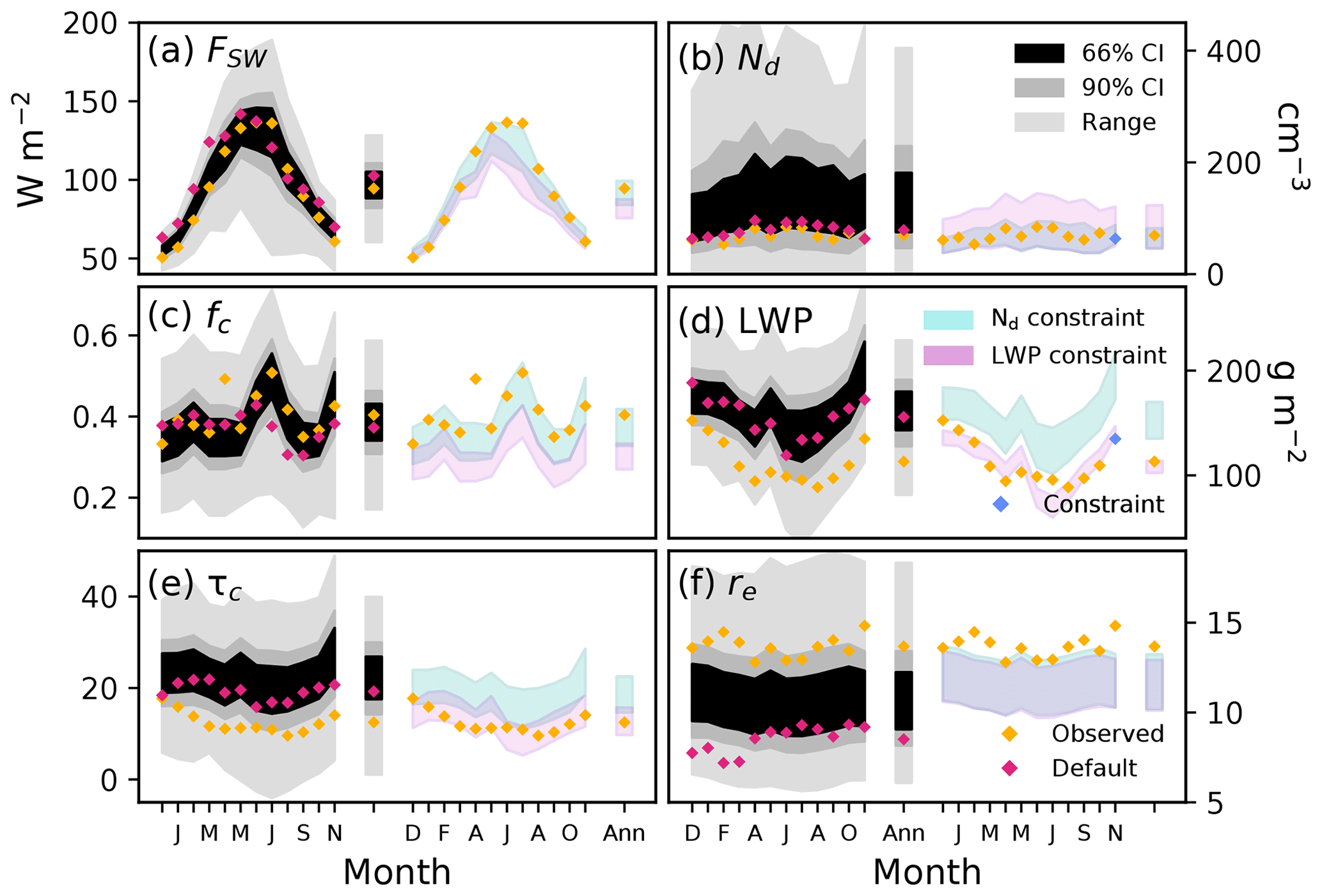
Figure 4 Seasonal cycles of North Atlantic mean radiative fluxes and cloud properties before and after observational constraint using a single month of observations. Model output for individual months spanning December 2016 to November 2017 are followed by the annual mean. Credible intervals for the full set of model variants are shown (grey shading) along with satellite-derived observations and the default UKESM1-A model values. Each panel also shows the range (shading) of values from the November N_d constraint (green) and the November LWP constraint (pink). The blue data points show the observed variable and month used for the constraint.

We identified instances of the second indicator of potential structural inadequacy (associated with inconsistent model process representations) by evaluating how the constraint of each model variable affects all other variables. We call this “pairwise” comparison. Figure 4 shows two contrasting sets of pairwise comparisons, highlighting both consistency and inconsistency. We constrained the model to match the mean N_d observation for November in the North Atlantic and, separately, to match November LWP observations in this region. November was chosen to exemplify the effect of the second indicator of potential structural inadequacy because the parametric uncertainty in N_d and LWP peaks in this month. In each case, we ruled out model variants with relatively large model–observation differences (quantified using NADs) as observationally implausible and retained the subset of model variants with values closest to observations (Sect. 2.4.5). Individual constraint variables have a large effect on the uncertainty of the same observation type in other months because they share common causes of uncertainty in the model. For example, the constraint to November N_d consistently reduces N_d uncertainty in all other months and brings the remaining model variants into close agreement with measured N_d values. This set of model variants also closely matches F_SW and f_c observations, with the exception of April f_c, which we have already identified as problematic.

These pairwise comparisons suggest that representations of N_d, F_SW, and f_c are internally consistent in the model, and we may only need a subset of these constraint variables to reduce uncertainty in ΔF_aer. However, the set of N_d-constrained model variants does not span the LWP, τ_c, or r_e observations in most months, suggesting that model N_d is inconsistent with LWP, τ_c, and r_e over the North Atlantic. In the other constraint shown in Fig. 4, the model variants that are consistent with November LWP in the North Atlantic do not span F_SW, f_c, or r_e observations. Retrievals of cloud properties are consistent by design due to dependencies in their calculation. That is, multiple retrieved cloud properties from the same instrument share causes of observation bias. Thus, our results suggest structural deficiencies in the model related to internal inconsistencies in the representations of physical and radiative cloud properties, which may be caused by the use of a single-moment cloud microphysics scheme in UKESM1. For example, in a single-moment microphysics scheme where N_d is not prognosed, removal of cloud water in precipitation (affecting LWP and τ_c) does not act consistently on N_d, which is prescribed by aerosol activation at the cloud base. Using a double-moment microphysics scheme, such as the Cloud–AeroSol Interacting Microphysics (CASIM) scheme (e.g. Grosvenor and Carslaw, 2020; Grosvenor et al., 2017; Hill et al., 2015; Shipway and Hill, 2012; Gordon et al., 2018), that simulates cloud water (droplet mass) and droplet number in a more realistic way could eliminate these internal model inconsistencies. However, in our ensemble, these inconsistencies may prevent us from using all available data for the constraint of ΔF_aci.

To reveal the full extent of internal model consistencies and inconsistencies, we extended the analysis in Fig. 4 to all pairwise comparisons of the 88 North Atlantic constraint variables and the 14 H_d constraint variables (Fig. 5; other regions are shown in Figs. S8–S11). The calculation of each of these pairwise effects across the full parameter space requires 1 million model-to-observation comparisons for each variable that is constrained and another 1 million for each variable being compared. Two constraint variables are judged to be pairwise consistent if constraint to one variable improves the model–observation comparison for the other variable and vice versa. We quantify the impact on model–observation comparison as the percentage change in the average NAD when moving from the unconstrained set of 1 million model variants to the set of model variants retained by the constraint (Sect. 2.4.2). For each pairwise comparison, the green shading in Fig. 5 indicates that observational constraint of the variable on the y axis improves the model–observation agreement (reduces average NAD) for the variable on the x axis. The pink shading indicates that the average NAD increases, which suggests that the two variables are inconsistent – that is, the set of model variants that best match the variable on the y axis is, on average, further from observations related to the variable on the x axis than in the original (unconstrained) set. For example, model skill in terms of simulating April f_c declines after constraint of any other variable, even f_c in most other months (vertical pink stripe). This supports our hypothesis that an observational error is the cause of the April f_c discrepancy and rules out the use of this constraint variable. These pairwise comparisons of constraint effects reveal inconsistencies between the model variables LWP, τ_c, and r_e and other variables related to cloud properties (F_SW, N_d, and f_c) in the North Atlantic (top-right quadrant and bottom-right panel of Fig. 5) and other regions (Figs. S8–S11). The degree of cross-variable consistency is not dependent on emulator skill (Fig. S1). We have identified two distinct sets of model variants that can be constrained independently but not in a consistent manner.

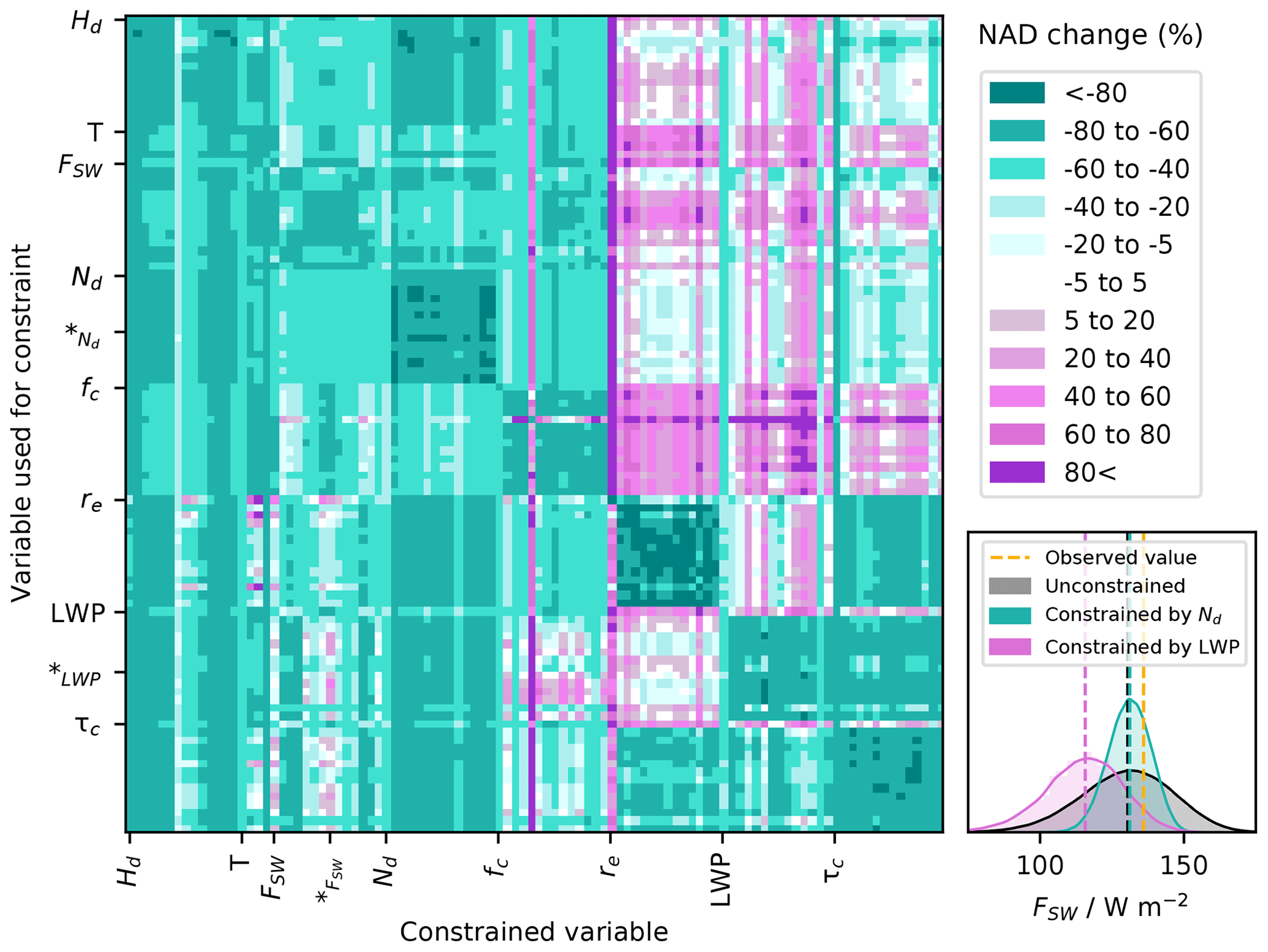
Figure 5 Pairwise comparisons of North Atlantic constraint variables (and hemispheric difference, H_d) showing how constraint of one variable affects all others. The y-axis labels refer to variables used to constrain the model output, and the x-axis labels refer to variables whose values have been consequently constrained. For each state variable, the pixels in the first row and/or column are the seasonal amplitude, followed by individual months from January to December and the annual mean. Transect variables are within the section labelled “T”. Shading indicates the percentage change in average NAD after constraint. In the bottom-right panel, we exemplify the effect of constraint on average NAD in two pixels (^*) in terms of probability density functions of July F_SW in the unconstrained set of model variants (black), in the set constrained to match July N_d observations (green), and in the set constrained to match July LWP (pink). Vertical dashed lines represent the observed F_SW value and median values in the unconstrained and constrained sets of model variants.

3.3.2 Optimal constraint of aerosol forcing

The pairwise comparisons in Fig. 5 show that it is not appropriate to use all observed variables to constrain the model because, due to potential structural model inconsistencies, different variables are consistent with different combinations of model parameters. The set of variants that simultaneously encompasses as many observed variables as possible is essentially the full initial set of 1 million. However, a smaller set of variants could be identified that agrees with those observed variables that are represented consistently in the model. This is an approach taken either deliberately or inadvertently in model tuning, in which some variables are deprioritised or neglected altogether. For example, F_SW is almost always treated as a high-priority target when tuning climate models because of its importance for energy balance, while N_d is more commonly treated as an adjustment term to achieve greater agreement with target values, and many other cloud variables are often neglected completely (e.g. Hourdin et al., 2017). Model-tuning approaches attempt to minimise the effect of biases in a well-configured model version rather than seeking to identify structural systematic biases across a large number of model variants, as we do here. There is no agreed best practice for identifying which combinations of model variables are structurally consistent. To explore the potential for constraint of ΔF_aci, we take the approach of constraining to the most consistent set of observed variables across our selected regions, then add more variables to understand the effect of accounting for inconsistencies.

We first identify constraint variables that are pairwise consistent with N_d at the regional level (see Sect. 2.4.4). We chose the 225 constraint variables that are N_d-pairwise consistent because N_d is one of the most uncertain variables we evaluate here (Fig. 4), and N_d is a common adjustment variable for ΔF_aer constraint (Hourdin et al., 2017) due to its sensitivity to aerosol and its importance for ΔF_aci. In practice, we could use other constraint variables to define an internally consistent set (top-left corner of Fig. 5). We evaluate the 25 200 combinations of these 225 constraint variables to reveal structural inconsistencies (Sect. 2.4.4). First, we identify the constraint variable with the greatest individual effect on reducing ΔF_aci uncertainty, then we progressively add constraint variables that are consistent with the existing set of variables (and N_d at the regional level) and contribute most to the ΔF_aci constraint. Figure 6 shows the effect of progressively adding constraint variables in this way (orange points).

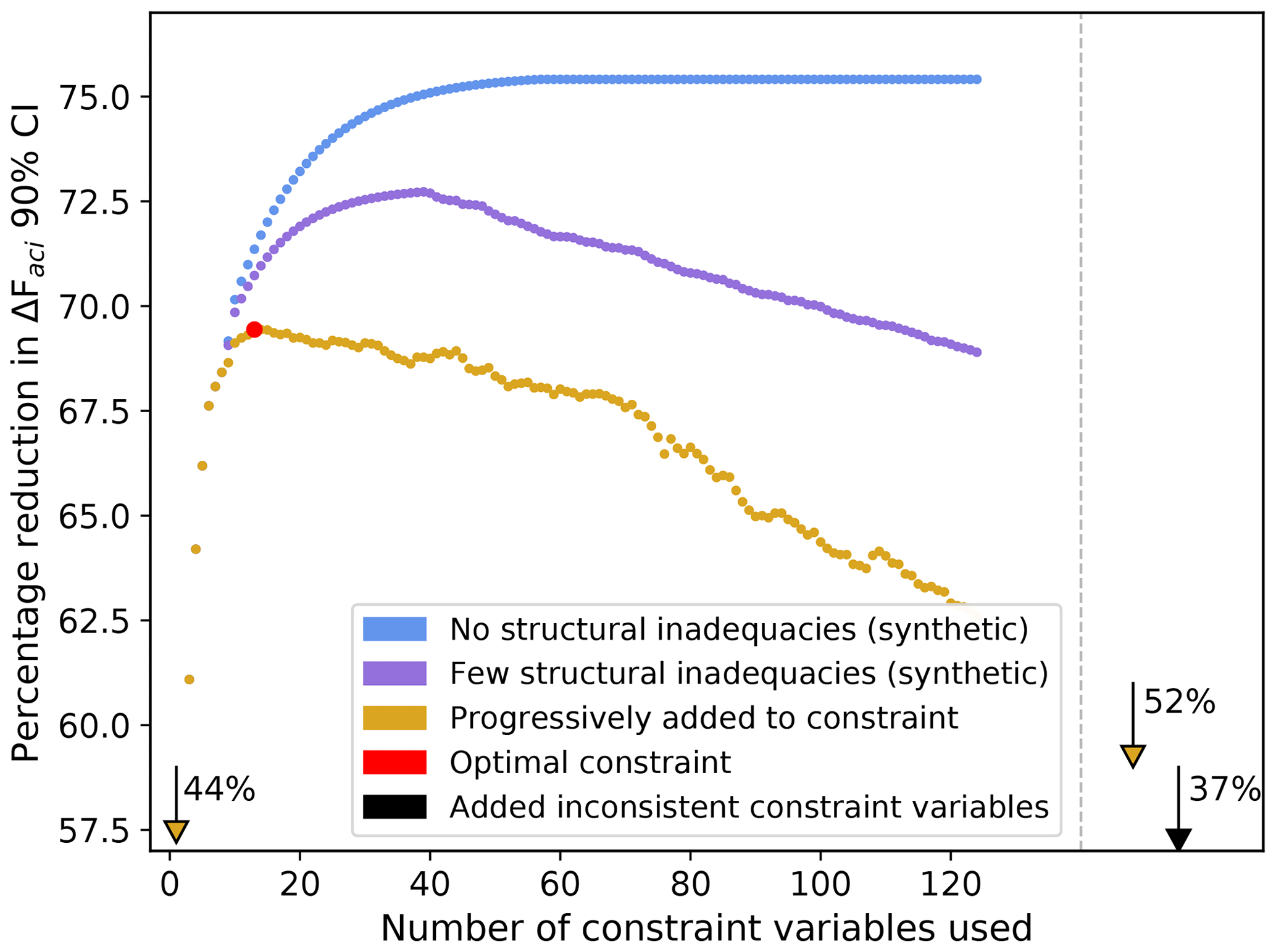
Figure 6 Constraint of ΔF_aci and the effect of varying the number of constraint variables used. We show the effect of progressively adding constraint variables with the greatest influence on ΔF_aci uncertainty (orange) alongside synthetic examples of how the constraint might improve with very few or no structural model inadequacies (purple and blue respectively). In each case, only the first 125 of 225 N_d-pairwise consistent constraint variables are shown. Arrows indicate the constraint of ΔF_aci using the single strongest constraint variable (44 %), all 225 N_d-pairwise consistent constraint variables (52 %), and all 450 constraint variables (37 %), including those associated with identified structural inadequacies at the regional level (e.g. Figs. 4 and 5).

The hemispheric contrast in N_d (H_d) in the Northern Hemisphere's summer (August) provides the strongest individual constraint on ΔF_aci. The constraint towards lower values of H_d in August reduces the credible ΔF_aci uncertainty range in the unconstrained set of model variants by around 44 %. August H_d shares causes of uncertainty with ΔF_aci and with H_d in all other months, but the nature of the relationships between the associated parameters (parameter dependencies) may be more clearly defined in August, since in most other months H_d is sensitive to additional parameters (Fig. S16). In combination with August H_d, additional constraint comes from next including South Pacific N_d in September (dependencies on natural emission flux parameters and dry deposition velocity) followed by March H_d (carbonaceous aerosol properties). Further constraint comes from North Pacific f_c in August (updraft velocity, autoconversion, and physical atmosphere parameters) and changes in LWP along the North Pacific transect (carbonaceous aerosol radiative properties, autoconversion, and physical atmosphere parameters). Southern Ocean N_d in December (natural emission fluxes and dry deposition velocities) and changes in LWP and N_d along the North Atlantic transect (updraft velocity and primary sulfate diameter) additionally constrain ΔF_aci.

Table 1 The 90 % credible intervals for ΔF_aer, ΔF_aci, and ΔF_ari from the original 1 million model variants and after constraint using process-based and energy balance methods. We also include plausible bounds (90 % credible interval) from energy balance constraints.

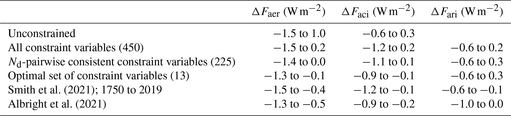
We only need to include 7 additional constraint variables in combination with the constraints identified above (13 in total) to optimally constrain ΔF_aci (i.e. greatest reduction in the ΔF_aci 90 % credible interval, red point in Fig. 6). We define the optimal constraint to be the greatest reduction in ΔF_aci achievable using our specified set of observations and structurally imperfect model. This optimal set of constraint variables spans the observation types, regions, and seasons and provides information about the key uncertain parameters associated with these observations (and ΔF_aci dependencies on key model parameters). The optimally constrained set of model variants reduces ΔF_aci uncertainty by nearly 70 % (90 % credible interval of −0.9 to −0.1 W m⁻²) and ΔF_aer uncertainty by more than 50 % (−1.3 to −0.1 W m⁻²; Fig. 2). This constrained ΔF_aer range is narrower than previous best estimates (Bellouin et al., 2020) and purely process-based constraints (Regayre et al., 2018, 2020; Johnson et al., 2020) even though the ΔF_ari component of forcing is effectively unconstrained here. Additionally, the optimally constrained lower negative bound is now in close agreement with energy balance constraints (Table 1).

When applied in combination with the set of the 13 optimal constraint variables, any additional variables weaken the constraint (Fig. 6). This is because the additional variables are either redundant (no additional benefit in reducing ΔF_aci uncertainty range because key parameter dependencies are already constrained), inconsistent with those already used (expand the parameter space and widen the uncertainty range), or some combination of these. We retain at least 5000 model variants for each combined constraint (Sect. 2.4.1), so the result of adding further observations can force a compromise in the sense that the existing constraints of ΔF_aci dependencies on key parameters need to be relaxed to accommodate conflicting information introduced by inconsistent variables. We hypothesise that the nature of this conflicting information could be revealed by exploring spatially and/or temporally coherent patterns of pairwise inconsistency. Practically, this compromise means that some of the model variants with low NAD values are no longer retained. Instead, these model variants are replaced with other variants that have tolerable (not low) NAD values for the existing set of constraint variables and tolerable NAD values in relation to the new variable. Thus, the constraint is no longer optimal (for our model and these observations). Including all 225 observations of N_d-pairwise consistent constraint variables reduces the ΔF_aci uncertainty by just over 50 %, and adding observations of inconsistent variables to the constraint reduces the uncertainty by less than 40 %. We expected a decline in constraint efficacy (levelling off when progressively adding constraint variables; Fig. 6) once hidden structural inconsistencies started to mitigate the benefits of including additional constraint variables. However, we did not anticipate that the optimal constraint would include so few constraint variables. These results suggest that, across 1 million variants, the model is structurally incapable of matching more than a handful of our chosen observations simultaneously (Fig. 6 and Table S4).

3.3.3 Constraint of uncertain model parameters

Our approach consistently constrains the values of model parameters (Figs. S12 and S13). Most parameters that cause ΔF_aci uncertainty (Fig. 3) are constrained, as are numerous other parameters that cause uncertainty in variables associated with our set of optimal observations that are not shared with ΔF_aci. We entirely rule out some values as observationally implausible for parameters related to vertical velocity and newly formed sulfate particle diameters. Vertical velocities are constrained towards lower values, which are consistent with lower N_d concentrations in the relatively polluted Northern Hemisphere, a lower hemispheric contrast in N_d, and weaker (less negative) median ΔF_aci. Conversely, newly formed sulfate particle diameters are constrained towards higher values, consistent with higher concentrations of cloud active aerosol concentrations and stronger (more negative) median ΔF_aci. Low sulfate emission diameters likely contributed to the spurious positive ΔF_aci values in Fig. 2. Dry deposition removal rates are also constrained towards higher values. This constraint reduces background aerosol concentration (consistent with lower N_d) and causes stronger (more negative) median ΔF_aci (increased sensitivity to anthropogenic aerosol). These key parameters are constrained concurrently, so they have the effect of ruling out the strongest and weakest ΔF_aci (and ΔF_aer) values in our original set of model variants.

There is little evidence to support altering the current model representations of natural emission fluxes. Two key causes of ΔF_aci uncertainty, the emission fluxes of sea spray aerosol and DMS, are constrained towards central values. However, the constraints on these parameters are relatively modest given their importance as causes of uncertainty. Additional constraint using in situ observations in relatively unpolluted regions (Hamilton et al., 2014; Schmale et al., 2019) could further constrain these parameters and the ΔF_aci uncertainty (Regayre et al., 2020). Also, additional ΔF_aer constraint could be achieved using in situ observations that target processes related to the ΔF_ari component of ΔF_aer (Johnson et al., 2020; Watson-Parris et al., 2020), which is effectively unconstrained by the satellite-derived observations used here.

4 Discussion

We illustrate some of the benefits of a climate model evaluation that accounts for parametric uncertainty. In addition to constraining the lower bound on ΔF_aer to −1.3 W m⁻², a value in close agreement with energy balance constraints, we have shown how this type of model evaluation can reveal potential structural model inadequacies. In our case, prioritising structural improvements to address model inconsistencies related to the representations of cloud variables would increase the number and type of observations that could be used to further reduce ΔF_aci and ΔF_aer uncertainty in the model.

Structural inconsistencies weaken model observational constraint because, to achieve tolerable agreement with more variables than in the optimal set, the inconsistencies demand a compromise in the tightness of constraint achieved (Fig. 7). In UKESM1-A, the set of optimal constraint variables is surprisingly small, containing only around 3 % of the constraint variables we explored. At present, the remaining 97 % of variables weaken the constraint. If we could make these variables consistent with other model variables already used for constraint, for example by altering the structure of the model, then they would instead potentially strengthen the constraint by further defining parameter relationships that were not constrained by the 3 %. The hypothetical lines in Fig. 6 (purple and blue) describe what might be achieved if some or all of the structural model inadequacies were identified and improved – moving the peak to the right (more constraint variables used consistently in a structurally different model) and raising the peak (tighter parametric constraint of ΔF_aci and ΔF_aer). The values used to create these lines are chosen to exemplify our point and do not correspond to actual constraints of the model. Ultimately, in a model without any structural inadequacies, the constraint versus number of variables would be an asymptote – additional variables would further constrain parameter relationships that were already partially constrained. The magnitude of constraint at this hypothetical asymptote is currently unknown. It will be determined in part by the effects of observational uncertainty and model–observation representation errors (Schutgens et al., 2017). Thus, we consider our optimal constraint to be the minimum level of process-based constraint that we might achieve with this set of observations if we could eliminate structural model inadequacies.

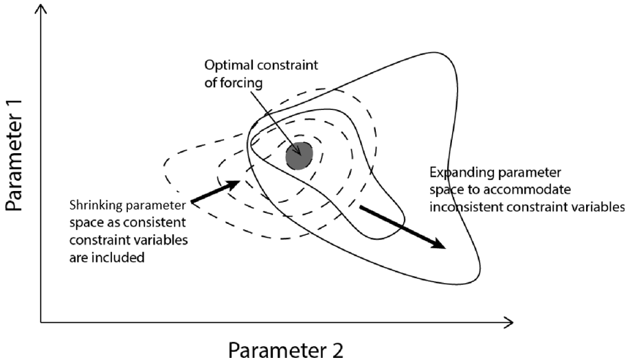
Figure 7 Schematic of how the addition of constraint variables affects the constrained parameter space. This is a 2-dimensional schematic of what is here a 37-dimensional problem. Initially, adding constraint variables leads to a reduction in the amount of parameter space that corresponds to a relatively good match to the observations (rising branch of Fig. 6). Each new variable constrains the parameter space more than the previous set. An optimum constraint is reached (grey-shaded region; peak in Fig. 6). Beyond this point, each new constraint variable is no longer consistent with the existing set already used because the model has structural deficiencies. Thus the parameter space must be expanded (and the ΔF_aer constraint weakened) to accommodate these inconsistencies.

We suggest that modelling groups may benefit from replacing existing model-tuning strategies with a new approach to model evaluation and development that accounts for parametric uncertainty and strategically identifies the causes of model inconsistencies as well as ways of overcoming their effects. In practice, the magnitude and distribution of observationally constrained ΔF_aer values in a structurally improved model may differ from the original model values (even with an identical set of parameter combinations). Thus, coherent progress in improving model skill in terms simulating aerosol–cloud interactions may require several cycles of uncertainty quantification, constraint, structural error identification, and model development. Open-source tools and code can help simplify some aspects of model evaluation within an uncertainty framework (Watson-Parris et al., 2021) and thus streamline some aspects of this cycle.

Identifying optimal replacements for inconsistent process representations will require additional insight into the causes of uncertainty within and across climate models, although the knowledge of inconsistencies between variables provided by our approach will provide a strong steer. This valuable insight could be achieved by extending model intercomparisons, such as the 6th Coupled Model Intercomparison Project (CMIP6; Eyring et al., 2016), to include a cross-model perturbed parameter component. Constraint of perturbed parameter uncertainty across multiple models will help close the gap between constrained model values of aerosol forcing and the real-world value. The breadth of model behaviour sampled in enhanced intercomparisons would help to identify optimal combinations of process representations and parameter values that minimise important shared biases in climate models. Additionally, data from such ensembles would be invaluable for training relatively simple climate models (Albright et al., 2021; Smith et al., 2021) and would contribute to efforts to identify robust emergent constraints (Carslaw et al., 2018). Experiments that sample parametric uncertainty and structural model differences could help deliver a step change in model skill in terms of making climate projections beyond the advances we have achieved here using a single climate model.