A new steady-state gas–particle partitioning model of polycyclic aromatic hydrocarbons: implication for the influence of the particulate proportion in emissions

Gas–particle (G–P) partitioning is a crucial atmospheric process for semi-volatile organic compounds (SVOCs), particularly polycyclic aromatic hydrocarbons (PAHs). However, accurately predicting the G–P partitioning of PAHs has remained a challenge. In this study, we established a new steady-state G–P partitioning model based on the level-III multimedia fugacity model, with a particular focus on the particulate proportion (ϕ₀) of PAHs in emissions. Similar to previous steady-state models, our new model divided the G–P partitioning behavior into three domains based on the threshold values of log K_OA (octanol–air partitioning coefficient), with slopes of 1, from 1 to 0, and 0 for the three domains. However, our model differed significantly from previous models in different domains. We found that deviations from the equilibrium-state G–P partitioning models were caused by both gaseous interference and particulate interference, with ϕ₀ determining the influence of this interference. Different forms of the new steady-state model were observed under different values of ϕ₀, highlighting its significant impact on the G–P partitioning of PAHs. Comparison of the G–P partitioning of PAHs between the prediction results of our new steady-state model and monitored results from 11 cities in China suggested varying prediction performances under different values of ϕ₀, with the lowest root mean square error observed when ϕ₀ was set to 0.9 or 0.99. The results indicated that the ϕ₀ was a crucial factor for the G–P partitioning of PAHs. Furthermore, our new steady-state model also demonstrated excellent performance in predicting the G–P partitioning of PAHs with entirely gaseous emission and polybrominated diphenyl ethers with entirely particulate emission. Therefore, we concluded that the ϕ₀ should be considered in the study of G–P partitioning of PAHs, which also provided a new insight into other SVOCs.

1 Introduction

The phenomenon of long-range atmospheric transport is capable of transporting semi-volatile organic compounds (SVOCs) from their sources to remote regions, such as the Arctic and the Tibetan Plateau, where they are neither produced nor utilized (Hung et al., 2005, 2010; C. Wang et al., 2018). The gas–particle (G–P) partitioning of SVOCs is an important atmospheric process that governs their fate and long-range transport (Zhao et al., 2020; Li et al., 2015). Furthermore, the distribution between the gas and particle phases plays a pivotal role in controlling the wet and dry depositions of SVOCs, thereby impacting the efficiency and extent of their long-range transport from sources to remote regions (Bidleman, 1988). Furthermore, the G–P partitioning of SVOCs is a significant issue for human exposure assessment, as gaseous and particulate SVOCs enter the human body through different routes (Weschler et al., 2015; Hu et al., 2021).

The G–P partitioning of SVOCs has been the subject of extensive research for several decades. Various models have been developed to predict the G–P partitioning coefficient (K_P) of SVOCs (Zhu et al., 2022; Qiao et al., 2020). Qiao et al. (2020) recently categorized eight G–P partitioning models into three groups: (1) models based on equilibrium-state theory (Pankow, 1987; Harner and Bidleman, 1998; Dachs and Eisenreich, 2000; Goss, 2005), (2) empirical models based on monitoring data (Li and Jia, 2014; Wei et al., 2017; Shahpoury et al., 2016), and (3) models based on steady-state theory (Li et al., 2015). Additionally, a new empirical model (equation) for polycyclic aromatic hydrocarbons (PAHs) (Zhu et al., 2022) and a new steady-state mass balance model for polybrominated diphenyl ethers (PBDEs) (Zhao et al., 2020) have recently been established. These models have been evaluated using field monitoring programs (Vuong et al., 2020; Qiao et al., 2019) and are frequently used to predict the G–P partitioning behavior of SVOCs (Qiao et al., 2020).

The G–P partitioning process of PAHs is more complex than that of other SVOCs due to concurrent particle formation (Dachs and Eisenreich, 2000; Shahpoury et al., 2016; Zhu et al., 2022). For instance, when the octanol–air partitioning coefficient (log K_OA) exceeds 12, the monitored values of K_P-M (monitoring data of G–P partitioning) of PAHs deviate from the predictions of both equilibrium-state and steady-state G–P partitioning models (Ma et al., 2020; Zhu et al., 2022). Recent studies have found that the particulate proportion (ϕ₀) of SVOCs in the emissions could affect the G–P partitioning of SVOCs (Qin et al., 2021; Zhao et al., 2020). As ϕ₀ increases, the predictions can diverge from the steady-state G–P partitioning model to the equilibrium-state G–P partitioning model (Qin et al., 2021; Zhao et al., 2020). Moreover, the emission sources of PAHs in the atmosphere are complex, including stationary sources (residential combustion, industrial production, and agricultural burning) and mobile sources (motor vehicles, railways, and shipping) (Zhang et al., 2020; Tang et al., 2020), in which both gaseous and particulate PAHs exist (Zimmerman et al., 2019; R. Wang et al., 2018; Shen et al., 2011; Cai et al., 2018b). Therefore, the detailed influence of ϕ₀ on the G–P partitioning of PAHs could be considered to explain the deviation of the measured K_P-M from both the equilibrium-state and the steady-state G–P partitioning model predictions.

In this study, we establish a new steady-state G–P partitioning model (hereafter referred to as the new steady-state model) based on the level-III multimedia fugacity model for PAHs and comprehensively discuss the influence of ϕ₀. Specifically, we (1) establish and deeply study the new steady-state model under different threshold values of log K_OA, (2) comprehensively discuss the influence of ϕ₀ on the G–P partitioning of PAHs, and (3) study the performance of the new steady-state model for prediction of K_P of PAHs.

2 Establishment of the new steady-state G–P partitioning model

2.1 Establishment method of the new steady-state model

In the current study, a steady-state six-compartment six-fugacity model was employed. The intricacies of this model can be found in Text S1 of the Supplement. The input and output fluxes of PAHs in both the gaseous and the particulate phases were graphically depicted in Fig. 1. The comprehensive computational techniques utilized to determine these fluxes are elaborated upon in Text S2.

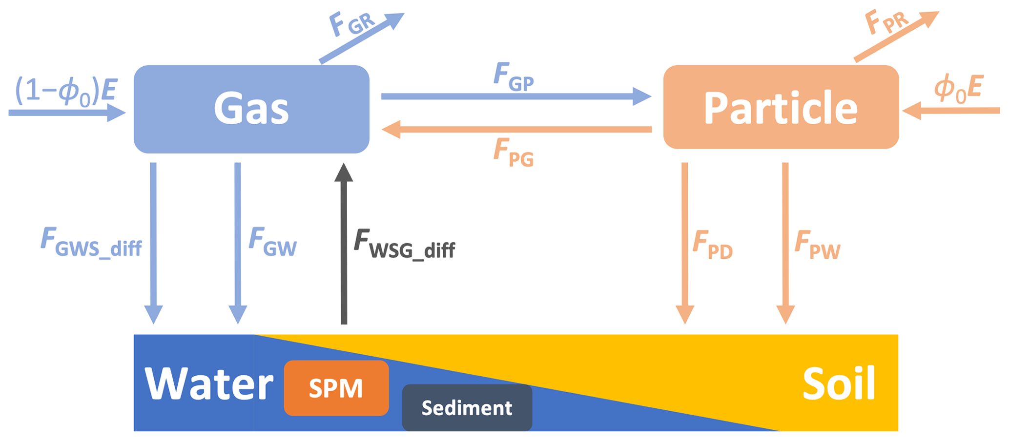
Figure 1 The fluxes related to the gas and particle phase in the six-compartment model. F_GR: degradation flux of gas-phase PAHs, F_PR: degradation flux of particle-phase PAHs, F_GP: migration flux from the gas phase to the particle phase, F_PG: migration flux from the particle phase to the gas phase, F_{GWS_diff}: diffusion fluxes from the gas phase to water and/or soil phases, F_GW: wet deposition flux of gas-phase PAHs to water and/or soil phases, F_{WSG_diff}: diffusion fluxes from soil and/or water phases to the gas phase, F_PD: dry deposition flux of particle-phase PAHs to suspended particle matter (SPM) in water phase and/or soil phase, F_PW: wet deposition flux of particle-phase PAHs to SPM and/or soil phases, (1−ϕ₀)E: emission flux of gas-phase PAHs, and ϕ₀E: emission flux of particle-phase PAHs.

Four groups were compared in terms of gas-phase and particle-phase input and output fluxes, namely input fluxes of the gas phase, output fluxes of the gas phase, input fluxes of the particle phase, and output fluxes of the particle phase. The results for PAHs were illustrated in Fig. S1. In order to establish a universal and concise model, the four fluxes (F_{GWS_diff}, F_{WSG_diff}, F_PR, and F_GW) were excluded from the system as their contributions were less than 10 % of the total fluxes. Furthermore, the special situation was not taken into account. For instance, even if the contribution of the flux of F_GW for dibenzo[a,h]anthracene (DahA) exceeded 10 %, it was still removed. After simplifying the function in Text S1, the two linear equations describing the input and output fluxes of the gas phase and the particle phase were established as follows:

$$\begin{array}{}\text{(1)}& \left\{\begin{array}{l}\left(\mathrm{1}-{\mathit{\varphi }}_{\mathrm{0}}\right)E+D_{\mathrm{GP}}{f}_{\mathrm{P}}=\left(D_{\mathrm{GR}}+D_{\mathrm{GP}}\right)f_{\mathrm{G}}\\ {\mathit{\varphi }}_{\mathrm{0}}E+D_{\mathrm{GP}}{f}_{\mathrm{G}}=\left(D_{\mathrm{GP}}+D_{\mathrm{PD}}+D_{\mathrm{PW}}\right)f_{\mathrm{P}},\end{array}\right.\end{array}$$

where f_P is the fugacity for particle-phase PAHs; f_G is the fugacity for gas-phase PAHs; D_GP is the intermedia D value between the gas phase and the particle phase; D_GR is the D value for the degradation of gas-phase PAHs; and D_PD and D_PW are the D values of the dry and wet depositions of particle-phase PAHs, respectively.

The fugacity ratio of the particle phase to the gas phase can be obtained by solving Eq. (1) as follows:

$$\begin{array}{}\text{(2)}& {\displaystyle \frac{f_{\mathrm{P}}}{f_{\mathrm{G}}}}={\displaystyle \frac{D_{\mathrm{GP}}+{\mathit{\varphi }}_{\mathrm{0}}{D}_{\mathrm{GR}}}{D_{\mathrm{GP}}+\left(\mathrm{1}-{\mathit{\varphi }}_{\mathrm{0}}\right)\left(D_{\mathrm{PD}}+D_{\mathrm{PW}}\right)}}.\end{array}$$

According to the fugacity method (Li et al., 2015) (see details in Text S3), the new steady-state model can be expressed as follows:

$$\begin{array}{}\text{(3)}& \begin{array}{rl}\log K_{\text{P-NS}}& =\log K_{\text{P-HB}}\\ & +\log \left({\displaystyle \frac{D_{\mathrm{GP}}+{\mathit{\varphi }}_{\mathrm{0}}{D}_{\mathrm{GR}}}{D_{\mathrm{GP}}+\left(\mathrm{1}-{\mathit{\varphi }}_{\mathrm{0}}\right)\left(D_{\mathrm{PD}}+D_{\mathrm{PW}}\right)}}\right).\end{array}\end{array}$$

In Eq. (3), log K_P-HB is the equilibrium-state G–P partitioning model (named the H–B model in this study, $\log K_{\text{P-HB}}=\log K_{\mathrm{OA}}+\log f_{\mathrm{OM}}-\mathrm{11.91}$; f_OM is the fraction of organic matter in particles, and K_OA is the octanol–air partitioning coefficient) (Harner and Bidleman, 1998). D_GR, caused by the degradation of PAHs in the gas phase, is defined as the gaseous interference, and D_PD+D_PW, caused by the deposition of PAHs in the particle phase, is defined as the particulate interference. The magnitude of this interference is determined by the value of ϕ₀.

By applying the calculation method of the D values in the multimedia fugacity model (Table S1) and the values of the related parameters in Tables S2, S3, S4, S5, and S6, Eq. (2) can be simplified as follows:

$$\begin{array}{}\text{(4)}& {\displaystyle \frac{f_{\mathrm{P}}}{f_{\mathrm{G}}}}={\displaystyle \frac{\mathrm{1}+\mathrm{13.2}{\mathit{\varphi }}_{\mathrm{0}}\times k_{\mathrm{deg}}}{\mathrm{1}+{\mathrm{10}}^{-\mathrm{10.31}}(\mathrm{1}-{\mathit{\varphi }}_{\mathrm{0}})f_{\mathrm{OM}}{K}_{\mathrm{OA}}}},\end{array}$$

where k_deg is the degradation rate of PAHs in the gas phase (h⁻¹).

Therefore, Eq. (3) can also be expressed as follows:

$$\begin{array}{}\text{(5)}& \begin{array}{rl}\log K_{\text{P-NS}}& =\log K_{\text{P-HB}}\\ & +\log \left({\displaystyle \frac{\mathrm{1}+\mathrm{13.2}{\mathit{\varphi }}_{\mathrm{0}}\times k_{\mathrm{deg}}}{\mathrm{1}+{\mathrm{10}}^{-\mathrm{10.31}}(\mathrm{1}-{\mathit{\varphi }}_{\mathrm{0}})f_{\mathrm{OM}}{K}_{\mathrm{OA}}}}\right).\end{array}\end{array}$$

Thus, it can be found that the new steady-state model (log K_P-NS) is a function of ϕ₀, k_deg, f_OM, and K_OA.

2.2 Different domains of the new steady-state model

Three domains have been delineated based on the threshold values of log K_OA. For example, if 10${}^{-\mathrm{10.31}}(\mathrm{1}-{\mathit{\varphi }}_{\mathrm{0}})f_{\mathrm{OM}}{K}_{\mathrm{OA}}\ll \mathrm{1}$, the initial threshold of log K_OA (log K_OA1) can be derived. Subsequently, Eq. (5) can be expressed as follows:

$$\begin{array}{}\text{(6)}& \log K_{\text{P-NS}}=\log K_{\text{P-HB}}+\log \left(\mathrm{1}+\mathrm{13.2}{\mathit{\varphi }}_{\mathrm{0}}\times k_{\mathrm{deg}}\right).\end{array}$$

In this domain, the value of log K_OA was less than log K_OA1, and log K_P-NS was a function of K_OA, f_OM, ϕ₀, and k_deg. As depicted in Fig. 2, the domain was illustrated with vertical lines serving as the backdrop. Notably, the prediction line of the new steady-state model was parallel to that of the H–B model within this domain.

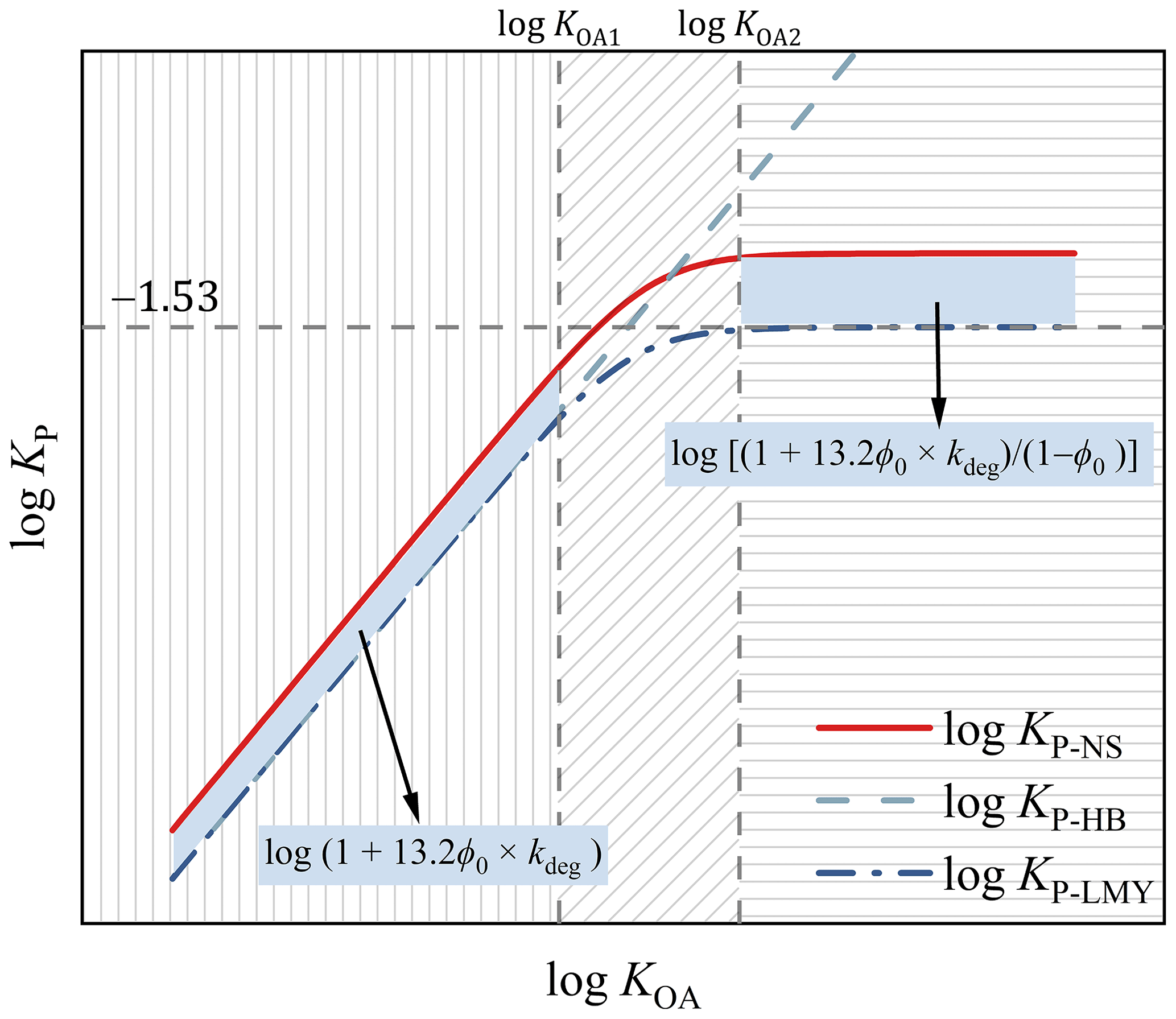
Figure 2 The three domains of the new steady-state G–P partitioning model divided by the two threshold values of log K_OA.

In addition, if 10${}^{-\mathrm{10.31}}(\mathrm{1}-{\mathit{\varphi }}_{\mathrm{0}})f_{\mathrm{OM}}{K}_{\mathrm{OA}}\gg \mathrm{1}$, the secondary threshold of log K_OA (log K_OA2) can be determined. Eq. (5) can be expressed as follows:

$$\begin{array}{}\text{(7)}& \begin{array}{rl}\log K_{\text{P-NS}}& =\log K_{\text{P-HB}}\\ & +\log \left({\displaystyle \frac{\mathrm{1}+\mathrm{13.2}{\mathit{\varphi }}_{\mathrm{0}}\times k_{\mathrm{deg}}}{{\mathrm{10}}^{-\mathrm{10.31}}(\mathrm{1}-{\mathit{\varphi }}_{\mathrm{0}})f_{\mathrm{OM}}{K}_{\mathrm{OA}}}}\right).\end{array}\end{array}$$

Through substitution of log K_P-HB using the equation $\log K_{\text{P-HB}}=\log K_{\mathrm{OA}}+\log f_{\mathrm{OM}}-\mathrm{11.9}$1 as proposed by Harner and Bidleman (1998), Eq. (7) can be simplified as follows:

$$\begin{array}{}\text{(8)}& \log K_{\text{P-NS}}=\log \left({\displaystyle \frac{\mathrm{1}+\mathrm{13.2}{\mathit{\varphi }}_{\mathrm{0}}\times k_{\mathrm{deg}}}{\mathrm{1}-{\mathit{\varphi }}_{\mathrm{0}}}}\right)-\mathrm{1.6}.\end{array}$$

Within this domain, the value of log K_OA was higher than log K_OA2; log K_P-NS was solely dependent on ϕ₀ and k_deg; and log K_P-NS reached a maximum constant value (log K_P-NSmax), as depicted by the section with horizontal lines in Fig. 2. Within this domain, the prediction line of the new steady-state model was parallel to that of the L–M–Y model.

Moreover, in the range where $\log K_{\mathrm{OA}\mathrm{1}}<\log K_{\mathrm{OA}}<\log K_{\mathrm{OA}\mathrm{2}}$, log K_P-NS exhibited a positive correlation with log K_OA, with a decreasing slope from 1 to 0 (Eq. 5). Within this domain, log K_P-NS was influenced by several factors, including K_OA, f_OM, ϕ₀, and k_deg. This particular range is depicted in Fig. 2 with a background of diagonal lines. Notably, within this domain, the prediction line of the new steady-state model closely resembled that of the L–M–Y model.

2.3 Difference between the new steady-state model and previous models

The dissimilarity between the new steady-state model and the H–B (Text S4) and L–M–Y models (the steady-state model) (Li et al., 2015) (Text S4) can be computed using Eq. (5) in different domains. In essence, as shown in Fig. 2, when log K_OA<log K_OA1, the contrast between the new steady-state model and the H–B model or the L–M–Y model can be denoted as ${\mathit{\delta }}_{\mathrm{1}}=\log (\mathrm{1}+\mathrm{13.2}{\mathit{\varphi }}_{\mathrm{0}}\times k_{\mathrm{deg}})$. The value of δ₁ increased along with the increase in ϕ₀ and reached the maximum value of log (1+13.2k_deg) when ϕ₀=1 (Fig. S2a). When log K_OA>log K_OA2, the difference between the new steady-state model and the L–M–Y model can be expressed as ${\mathit{\delta }}_{\mathrm{2}}=\log \left[\right(\mathrm{1}+\mathrm{13.2}{\mathit{\varphi }}_{\mathrm{0}}\times k_{\mathrm{deg}})/(\mathrm{1}-{\mathit{\varphi }}_{\mathrm{0}}\left)\right]$. The value of δ₂ also increased along with the increase in ϕ₀ and approached infinity when ϕ₀ is infinitely close to 1 (Fig. S2b). When $\log K_{\mathrm{OA}\mathrm{1}}<\log K_{\mathrm{OA}}<\log K_{\mathrm{OA}\mathrm{2}}$, the difference between the new steady-state model and the L–M–Y model was the function of ϕ₀ and K_OA, which increased along with the increase in ϕ₀ and K_OA. Further information can be found in the subsequent section.

3 Influence of ϕ₀ on K_P of PAHs

In general, varying values of ϕ₀ correspond to distinct configurations of the new steady-state model (Eq. 3). Specifically, three different forms can be obtained depending on the values of ϕ₀: $\mathrm{0}<{\mathit{\varphi }}_{\mathrm{0}}<\mathrm{1}$, ϕ₀=0, and ϕ₀=1.

When $\mathrm{0}<{\mathit{\varphi }}_{\mathrm{0}}<\mathrm{1}$, both the particulate and the gaseous PAHs are present in the emission, and the new steady-state model is expressed as Eq. (3). In this form, it is necessary to consider both gaseous interference and particulate interference for the G–P partitioning of PAHs in the atmosphere. The deviation of the new steady-state model from the H–B model depends on the ratio of ϕ₀D_GR to $(\mathrm{1}-{\mathit{\varphi }}_{\mathrm{0}})(D_{\mathrm{PD}}+D_{\mathrm{PW}})$. When the ratio exceeds 1, log K_P-NS deviates upwards from the prediction of the H–B model, whereas log K_P-NS deviates downwards when the ratio is lower than 1.

When ϕ₀=0, the PAHs in the emission are entirely in the form of gaseous PAHs, and Eq. (3) can be expressed as follows:​​​​​​​

$$\begin{array}{}\text{(9)}& \log K_{\text{P-NS}}=\log K_{\text{P-HB}}+\log \left({\displaystyle \frac{D_{\mathrm{GP}}}{D_{\mathrm{GP}}+\left(D_{\mathrm{PD}}+D_{\mathrm{PW}}\right)}}\right).\end{array}$$

Indeed, this equation is identical to that of the L–M–Y model, wherein α is defined as $D_{\mathrm{GP}}/(D_{\mathrm{GP}}+D_{\mathrm{PD}}+D_{\mathrm{PW}})$ (Li et al., 2015).

When ϕ₀=1, the PAHs in the emission are entirely in the form of particulate PAHs, and Eq. (3) can be expressed as follows:

$$\begin{array}{}\text{(10)}& \log K_{\text{P-NS}}=\log K_{\text{P-HB}}+\log \left({\displaystyle \frac{D_{\mathrm{GP}}+D_{\mathrm{GR}}}{D_{\mathrm{GP}}}}\right).\end{array}$$

The disparity of the new steady-state model from the H–B model can primarily be attributed to the degradation of PAHs in the gas phase. In cases where k_deg is negligible, the new steady-state model is equivalent to the H–B model.

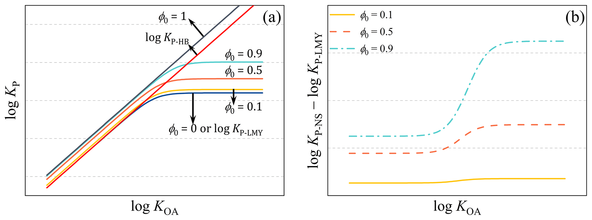
Figure 3 The comparison between the new steady-state model and the H–B model and the L–M–Y model. (a) The prediction lines of the three models; (b) the difference between the new steady-state model and the L–M–Y model with different values of ϕ₀.

The impact of ϕ₀ on K_P-NS of PAHs was investigated by analyzing different values of ϕ₀, and the results are presented in Fig. 3. As depicted in Fig. 3a, the prediction line of the new steady-state model diverged from the L–M–Y model towards the H–B model as ϕ₀ increased, which was consistent with previous studies (Zhao et al., 2020; Qin et al., 2021). In addition, obvious differences were observed between the prediction lines for the three models. Notably, when ϕ₀=1, the line of log K_P-NS was parallel to the line of log K_P-HB. When ϕ₀=0, the prediction line of log K_P-NS was identical to that of log K_P-LMY. When $\mathrm{0}<{\mathit{\varphi }}_{\mathrm{0}}<\mathrm{1}$, the trend of the prediction lines of log K_P-NS was similar to that of log K_P-LMY. The deviation between the prediction lines of log K_P-NS and log K_P-LMY is illustrated in Fig. 3b. Generally, the deviations between the prediction lines varied with the values of ϕ₀ and log K_OA. Additionally, the deviation increased with the increase in ϕ₀ and exhibited three distinct trends with the increase in log K_OA, separated by the two threshold values of log K_OA (log K_OA1 and log K_OA2).

4 Validation of the new steady-state G–P partitioning model

4.1 Validation

As is widely acknowledged, the sources of atmospheric PAH emission are multifaceted, encompassing both stationary sources and mobile sources (Zhang et al., 2020). Moreover, varying proportions of particulate PAHs have been reported across different emission sources (Zimmerman et al., 2019; R. Wang et al., 2018; Shen et al., 2011; Cai et al., 2018b). As a result, determining precise values of ϕ₀ is no easy feat. In this section, we consider different values of ϕ₀ (0, 0.1, 0.5, 0.9, 0.99, and 1) in conjunction with the new steady-state model for predicting K_P-M of PAHs, in order to obtain representative results.

To assess the performance of the new steady-state model, the monitored log K_P-M values of PAHs from 11 cities across China were utilized (Ma et al., 2018, 2019, 2020). As depicted in Fig. 4, the prediction line of the new steady-state model exhibited a remarkable concurrence with the monitoring data of log K_P-M. Notably, for the monitoring data with high log K_OA, the data were predominantly distributed between the prediction lines of the steady-state model with the values of ϕ₀ from 0 to 1. Furthermore, for different cities (Fig. S3), the values of ϕ₀ for the best-matched prediction lines of the new steady-state model varied, which was anticipated, since the sources of PAHs also differed among the 11 cities. The degree of concurrence of the new steady-state model was also evaluated using the root mean square error (RMSE) method (Text S5). Generally, for PAHs with high values of log K_OA (such as the high-molecular-weight PAHs), when ϕ₀ was set to 0.9 or 0.99, the value of RMSE for each city was the lowest (Fig.  S4), indicating the best degree of concurrence between the prediction results and the monitoring results. In fact, previous studies have shown that high-molecular-weight PAHs were dominant in the particle phase in emissions with higher ϕ₀ (Shen et al., 2011; Mastral et al., 1996; Lu et al., 2009), which lends credence to our findings.

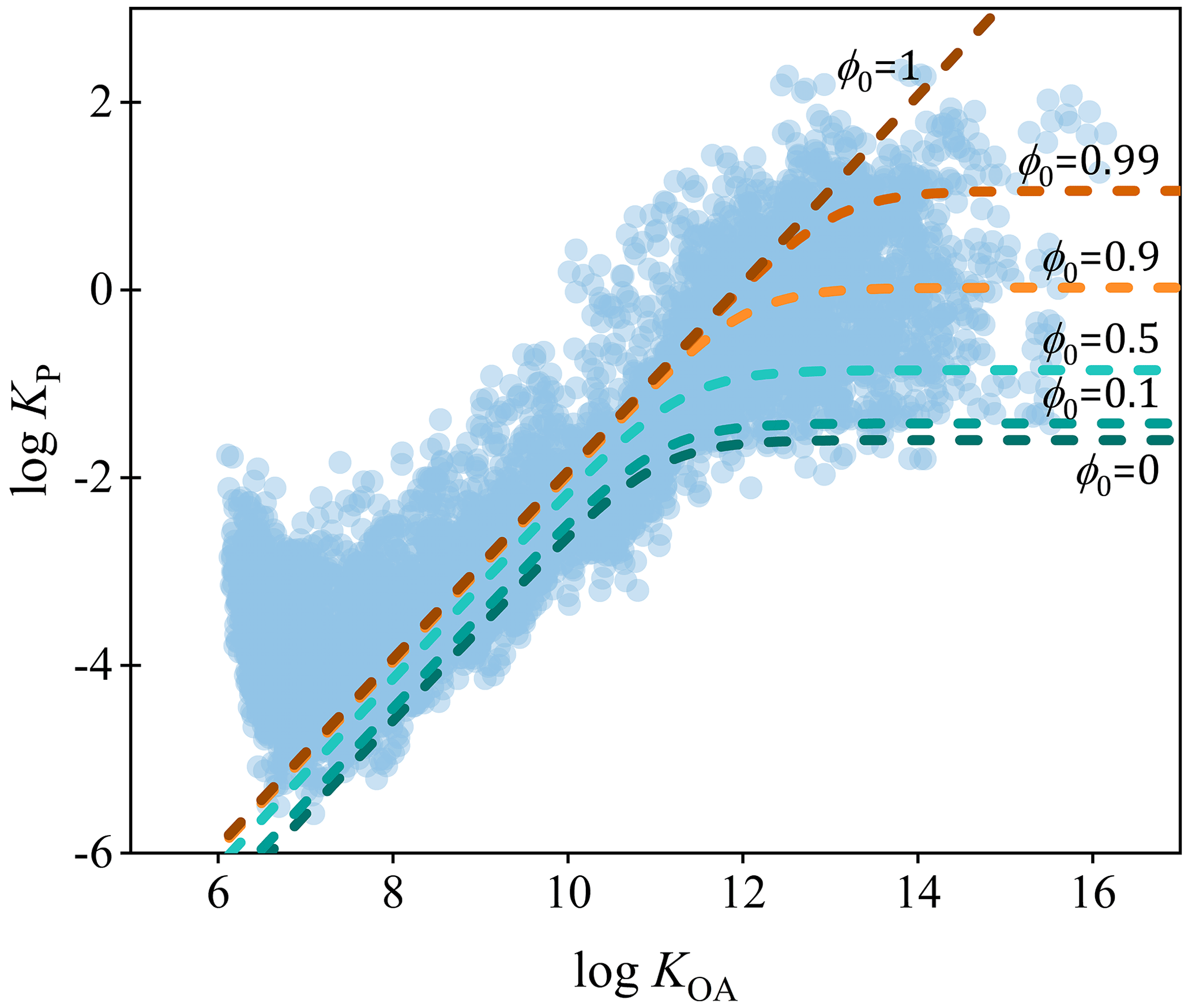
Figure 4 The comparison between the monitored data of log K_P-M of PAHs from 11 cities in China and the prediction lines of the new steady-state model with different values of ϕ₀.

Moreover, the performance of the new steady-state model in predicting log K_P-M of PAHs in a special scenario was also examined. Notably, in the prototype coking plant, the dust removal efficiency was an impressive 96 % (Liu et al., 2019). In this scenario, the gaseous PAHs were the primary source of emissions, and the values of ϕ₀ were approximately 0. As illustrated in Fig. S5, the monitored data of log K_P-M from the coking plant aligned most closely with the prediction line of the new steady-state model with ϕ₀=0, exhibiting the lowest RMSE. Based on this comparison, the optimal ϕ₀ in the steady-state model was consistent with that in the emission profile. This finding underscored the exceptional performance of the new steady-state model in this unique scenario.

It is possible to extend the steady-state model to other SVOCs by taking into account their comparable partitioning characteristics, while the model was originally developed based on the parameters of PAHs. To validate the performance of the new steady-state model for other SVOCs, a special scenario involving the recycling of electrical and electronic waste (e-waste) sites was considered. In this case, PBDEs were predominantly found in the particle phase of emissions, and the value of ϕ₀ was estimated to be approximately 1 (Cai et al., 2018a). Fig. S6 depicts the comparison between the monitored data of log K_P-M from several e-waste sites (Tian et al., 2011; Han et al., 2009; Chen et al., 2011) and the prediction lines of the new steady-state model with varying values of ϕ₀ (0, 0.1, 0.5, 0.9, 0.99, and 1). The corresponding results for RMSE are presented in Fig. S7. Notably, the monitored data of log K_P-M exhibited the best agreement with the prediction line of the new steady-state model with ϕ₀=1, which also had the lowest values of RMSE. Thus, it can be inferred that the new steady-state model can be expanded to predict the K_P-M of PBDEs in e-waste sites.

4.2 Implication

The present study has introduced a new steady-state G–P partitioning model, which incorporates the particulate proportion of SVOCs in emissions. In essence, the study has shed new light on the field of G–P partitioning and other related disciplines involving SVOCs. Firstly, in cases where SVOCs in the atmosphere originate from diverse emission sources with varying ϕ₀, the new steady-state model is more appropriate for the G–P partitioning study and other related assessments, such as those pertaining to health risks. Secondly, when examining the pollution characteristics and regional transport of SVOCs from a single point source, such as the transport of PBDEs around an e-waste site or the transport of SVOCs around chemical factories, the G–P partitioning of SVOCs must account for the particulate fraction of SVOCs in emissions. Thirdly, for long-range atmospheric transport studies, if there are multiple sources of SVOCs along the transport way, the continuous impact of the particulate fraction of SVOCs in emissions on the transport and fate of SVOCs needs careful consideration, such as the development of an atmospheric transport model.

4.3 Limitation

In light of the foregoing discussion, it can be inferred that the new steady-state model exhibited commendable performance in predicting K_P-M of PAHs in diverse real-world atmospheres, thereby providing a fresh avenue for investigating the G–P partitioning of PAHs and other SVOCs. Nonetheless, certain limitations of the new steady-state model persisted in the present study. Firstly, the values of ϕ₀ varied across different compounds and different emission sources (Zimmerman et al., 2019; R. Wang et al., 2018; Shen et al., 2011; Cai et al., 2018b). In the present study, constant values of ϕ₀ were employed for the new steady-state model, which were merely considered to be special examples. The precise values of ϕ₀ should be utilized for the application of the new steady-state model in the future. Secondly, for k_deg and f_OM, only one constant and common value was employed for the new steady-state model. Generally, these two parameters were also complex in the real atmosphere. For example, k_deg was related not only to the physicochemical properties of chemicals, but also to the environmental parameters, such as temperature and concentration (Wilson et al., 2021). Moreover, even though the f_OM can be directly measured, the actual values of f_OM also fluctuated with various factors, such as emission sources (Gaga and Ari, 2019; Lohmann and Lammel, 2004) and particle sizes (Hu et al., 2020). To evaluate the impact of the three parameters on K_P-NS in the new steady-state model, the sensitivity analysis was conducted via a Monte Carlo analysis with 100 000 trials employing the commercial software package Oracle Crystal Ball. To obtain comprehensive results, the sensitivity analysis was conducted for different values of log K_OA from 6 to 16. As presented in Fig. S8, it is noteworthy that three different ranges of log K_OA were observed based on different characteristics. For the range of log K_OA from 6 to 10, the influence of ϕ₀ dominated followed by k_deg and f_OM. Furthermore, for each parameter, the influence remained stable for different log K_OA values in this range. For the range of log K_OA from 10 to 12, the influence of ϕ₀ dominated followed by k_deg and f_OM. Additionally, the influence of ϕ₀ increased, while for the other two parameters the influence decreased. In the third range of log K_OA (12 to 16), the influences of the three parameters remained stable. Moreover, the influence of ϕ₀ dominated, and the influence of f_OM can be disregarded. In fact, the three ranges of log K_OA were consistent with the three domains. It can be concluded that the different influences of the three parameters on K_P-NS for different log K_OA values should be considered for the new model. Therefore, the precise values of ϕ₀, k_deg, and f_OM for the real atmosphere should be employed for the application of the new steady-state model in the future.

Furthermore, the new steady-state model was established based on a single multimedia environment, in which the advections of air and water were not considered. Additionally, some fluxes were removed to simplify the parameters of the model. Therefore, the influence of all fluxes and parameters related to gas and particle compartments should comprehensively be evaluated in the future. Furthermore, the validation and implication of the new steady-state G–P partitioning model should also be conducted for other SVOCs in a real multimedia environment.