Daytime along-valley winds in the Himalayas as simulated by the Weather Research and Forecasting (WRF) model

Local along-valley winds in four major valleys on the southern slope of the Nepal Himalayas are studied by means of high-resolution meteorological modelling. The Weather Research and Forecasting model is run with a 1 km horizontal grid spacing covering a 4 d period in December 2014. Model evaluation against meteorological observations from three automatic weather stations in the Khumbu Valley (one of the four valleys) shows a good agreement between the modelled and observed daily cycle of the near-surface wind speed and direction. Well-defined daytime up-valley winds are found in all of the four valleys during this 4 d period. The night-time along-valley winds are weak in magnitude and flow mostly in the up-valley direction. Differences in the daytime up-valley winds are found between the valleys and their parts. As the valleys are under similar large-scale forcing, the differences are assumed to be due to differences in the valley topographies. Parts of the valleys with a steep valley floor inclination (2–5^∘) are associated with weaker and shallower daytime up-valley winds compared with the parts that have nearly flat valley floors (<1^∘). In the four valleys, the ridge heights also increase along the valley, meaning that the valley floor inclination does not necessarily lead to a reduction in the volume of the valley atmosphere. This way, the dominant driving mechanism of the along-valley winds, within the valleys, could shift from the valley volume effect to buoyant forcing due to the inclination. Two of the valleys have a 1 km high barrier in their entrances between the valley and the plain. Winds at the valley entrances of these two valleys are weaker compared with the open valley entrances. Strong and shallow winds, resembling down-slope winds, are found on the leeward slope of the barrier followed by weaker and deeper winds at the valley entrance, 20 km towards the valley from the barrier. Although the large-scale flow during the 4 d period was similar to the long-term climatology, the impact of different large-scale flows on the thermally driven winds was not considered. This topic could be addressed in the future by performing a longer simulation.

1 Introduction

Day-to-day weather in mountain valleys is affected by thermally driven local winds that commonly form under clear skies. The formation of these winds are sensitive to, for example, any large-scale forcing (Whiteman and Doran, 1993) and the geometry of the valley topography (Wagner et al., 2015) which makes them unique for each and every valley. Plain-to-valley winds, and further along-valley winds, stem from the uneven warming of the valley atmosphere and the air above the adjacent plain. The temperature difference causing the along-valley winds is explained by the valley volume effect (Whiteman, 2000). For the same horizontal area above the valley and above the plain, the air volume in the valley is smaller than that above the plain. With the same given solar heating, the valley atmosphere will warm more than the air above the plain which creates a pressure gradient between the plain and the valley. The daytime cross-valley winds, on the other hand, are driven by the buoyancy force that arises from the horizontal temperature difference between the air immediately adjacent to the slopes, which is heated, and the air on the same horizontal level but away from the slope.

In real valley atmospheres, the mechanisms driving along- and cross-valley winds together lead to a three-dimensional valley circulation: during the daytime, the air flows up the slopes and valleys and from the plain into the valley. The daytime cross-valley circulation consists of up-slope winds in the near-surface layer and subsidence in the valley atmosphere away from the slopes. Subsidence warming is the dominant mechanisms leading to the heating of the air in the core of the valley in the morning transition phase, whereas the turbulent convective heat flux from the valley floor and the slopes is the dominant mechanism in the afternoon (Serafin and Zardi, 2010). Similarly, the up-slope winds typically form just after sunrise, peaking before noon, whereas the up-valley winds develop later during the day and peak in the afternoon (Whiteman, 2000). Although in the cross-valley circulation the subsiding air causes local warming in the core of the valley atmosphere, the net effect of the cross-valley circulation is to export heat out of the valley atmosphere due to the overshooting up-slope winds at the valley crests (Schmidli, 2013). Due to the heat export, the valley volume effect is considered to be the theoretical maximum of the heating of the valley atmosphere compared with adjacent plain.

Accurate modelling of these thermally driven winds requires high horizontal resolution, down to at least a 1 km grid spacing, due to their complex structure and sensitivity to the topography (Schmidli et al., 2018). The local valley circulation, as well as the vertical exchange of heat and momentum between the valley and the free troposphere, is inaccurately modelled in climate models that are typically run at a coarse resolution of up to 100–200 km (Rotach et al., 2014). With coarse-resolution models, it is also not possible to accurately simulate the vertical transport of aerosol emitted in the mountain boundary layer and ventilated by the valley winds into the free troposphere. Once in the free troposphere, aerosols are less subject to removal processes and can undergo chemical transformation and long-range transport; thus, ventilated aerosols can effect areas remote from the actual valley in which they were formed. As over half of the Earth's land surface is considered to be complex terrain (Rotach et al., 2014), this creates a high uncertainty, for example, in the global carbon budget and in climate change predictions.

This study concentrates on four valleys located in the Nepal Himalayas during a 4 d period in December 2014. The local wind patterns in Khumbu Valley (one of the valleys that is investigated in this study) have been studied in the past by means of meteorological observations (Inoue, 1976; Ueno and Kayastha, 2001; Bollasina et al., 2002; Ueno et al., 2008; Bonasoni et al., 2010; Shea et al., 2015; Yang et al., 2018) and high-resolution meteorological modelling (Karki et al., 2017; Potter et al., 2018, 2021). Overall, the daily cycle of the along-valley winds in Khumbu Valley are similar among existing studies, with well-defined daytime up-valley winds and weaker night-time winds flowing either in the up- or down-valley direction. A recent study showed that Khumbu Valley could act as a source of pre-industrial aerosol in the free troposphere: model results indicate that the biogenic vapours emitted in Khumbu Valley were oxidised and then transported to free troposphere by the daytime up-valley winds (Bianchi et al., 2021). They suggest that other similar valleys on the southern slope of the Himalayas would likewise form and transport biogenic aerosol to the free troposphere. However, the local valley wind systems in the other major valleys located nearby have not yet been well studied. Therefore, it remains unknown if these other major valleys have similar along-valley winds to those found in Khumbu Valley and, thus, if they could also act as sources of free-tropospheric aerosol.

This study focuses on along-valley winds during a carefully selected 4 d period in December 2014 that is representative of the post-monsoon season. The first aim of this article is to identify the characteristics (wind speed, depth of the flow and diurnal cycle) of the local valley wind system in four major valleys in the Hindu Kush–Karakoram–Himalayan (HKKH) region during this 4 d period in December 2014. The second aim is to identify notable differences between the four valleys in terms of their local wind systems. The third aim is to attempt to explain the causes for the differences in the local winds. These aims are addressed primarily by analysing a 4 d simulation performed with the Weather Research and Forecasting (WRF) model, as the network of meteorological observations is rather scarce in this region.

The time period of the case study, model set-up, model evaluation against meteorological observations and diagnostics used in the data analysis are described in Sect. 2. The valley topographical characteristics are described in Sect. 3. The along- and cross-valley wind characteristics in each of the four valleys are described in Sect. 4. The differences in the valley winds between the valleys are discussed in Sect. 5, and the conclusions are given in Sect. 6.

2 Methods

2.1 Time period of the case study

Due to computational and data storage limitations, it is not possible to perform a long-term simulation with high-temporal-resolution output. Therefore, in this study, we do not attempt to provide a climatology of the thermally driven winds. Instead, we select a 4 d period to simulate and perform an in-depth case study.

Bollasina et al. (2002) describe the seasonal variation and climatology of the study area by means of 6 years of meteorological observations made at the Nepal Climate Observatory – Pyramid (NCO-P) station, located close to the base of Mount Everest (marked as a black star in Fig. 2b). Generally, clear skies and daily temperature range maximums are observed in the month of December during the period from 1994 to 1999 at NCO-P (Bollasina et al., 2002). Similarly, during the 2006–2007 winter seasons (November–February, NDJF), clear skies and strong diurnal variation in temperature were observed by Bonasoni et al. (2010). Based on the observations at NCO-P, December is a good period for studying the thermally driven mountain winds in this region.

The period of this case study was selected to coincide with the measurement campaign by Bianchi et al. (2021) that took place in Khumbu Valley between 29 November and 25 December 2014, as additional observations and analysis of the local weather conditions were already available. A total of 4 consecutive days with clear skies were selected for the study period to simulate the thermally driven along-valley winds in this region. During the period from 18 to 21 December 2014, weather at the measurement site was reported to be sunny (supplementary material of Bianchi et al., 2021). Comparing the observed wind direction during the 18–21 December 2014 study period (Bianchi et al., 2021) with other periods, such as the winters of 1994–1999 (Bollasina et al., 2002; Ueno and Kayastha, 2001), December in 2003 (Ueno et al., 2008) and December in 2006 and 2007 (Bonasoni et al., 2010), the study period resembles the average wind conditions at the NCO-P station well.

To determine if the large-scale flow during our 4 d period is representative of the long-term climatology, we compare daily averages of upper-level winds from the study period to the 40-year climatology using the ERA5 reanalysis (Hersbach et al., 2020). The large-scale flow is examined at 400 hPa, as the surface pressure is below 500 hPa at many locations within the study area. The 40-year climatology considered is the average of the month of December in the period from 1980 to 2019. The 40-year average and the daily averages of the large-scale flow during the study period are shown in Fig. 1. The border of Nepal is shown in red in Fig. 1, and the study area is located in the north-eastern part of Nepal. The 40-year December average of the 400 hPa wind is mostly westerly with the subtropical jet located on average at around 30^∘ N. The subtropical jet is located around 25^∘ N during 18–21 December 2014, which is south-east of the study area. The jet seen in the 40-year average (Fig. 1a) is much wider than in any of the daily averages, suggesting that the exact latitudinal position of the jet varies from day to day. Although the jet is located around 5^∘ south of the 40-year average during our study period, the relatively large standard deviation implies that the study period is still representative of the area's climatological large-scale wind conditions. During 18–21 December 2014, the daily averaged wind speeds differ from the 40-year average by less than 1 standard deviation (SD) of the December monthly means near the study area (Fig. 1b, c, d, e).

Figure 1 (a) The 400 hPa wind speed (shading) and direction (white vectors) averaged over the month of December for the period from 1980 to 2019 in the ERA5 reanalysis. The standard deviation of the 40-year monthly means is shown by the black contours (m s⁻¹). (b–e) Daily averaged wind speed and direction at 400 hPa in the ERA5 reanalysis for the period from 18 to 21 December 2014. The standard score of the daily average wind speed compared to the 40-year monthly means is shown by the black contours with a contour interval of 1 SD. Coastlines and country borders are shown in grey, and the borders of Nepal are shown in red.

2.2 Weather Research and Forecasting model set-up

The Weather Research and Forecasting model (WRF) is a state-of-art numerical weather prediction model that is widely used for both operational and research purposes. The version used in this study is WRF 3.6.1.

The simulation used in this study is identical to the simulation that Bianchi et al. (2021) analysed in their study. The simulation consists of four nested domains (referred to as d01, which is the outer domain, and d02, d03 and d04, which comprise the inner domain) that are illustrated in Fig. 2a. The outer domain covers an area of 3618 × 2997 km and was run with a horizontal grid spacing of 27 km. The horizontal grid spacing decreases to 9 km (d02), 3 km (d03) and finally to 1 km in the innermost domain, which covers an area of 288 × 300 km. All of the domains are run with 61 vertical levels.

The simulation was initialised using the Climate Forecast System Reanalysis (Saha et al., 2010) which has a horizontal grid spacing of 0.5^∘. The simulation was kept on track by nudging the temperature, horizontal wind components and specific humidity in the outer domain (d01) towards the reanalysis every 6 h. The nudging was only performed above the atmospheric boundary layer. The surface topography is from United States Geological Survey with a horizontal resolution of 30 arcsec (∼ 1 km) and is shown for domains d01 and d04 in Fig. 2a and b respectively. An adaptive time step with a target Courant–Friedrichs–Lewy value of 0.8 was used to keep the simulation numerically stable. For the inner domain (d04), this means a time step of approximately 1 s. In addition, sixth-order numerical diffusion and w-Rayleigh damping were applied to the uppermost 5 km. Sub-grid-scale processes were parameterised as follows: the Thompson scheme for microphysics (Thompson et al., 2008), the Rapid Radiative Transfer Model for General Circulation Model (RRTMG) scheme for long-wave and short-wave radiation (Iacono et al., 2008), the Mellor–Yamada–Janjić (Eta) turbulent kinetic energy (TKE) scheme for boundary-layer turbulence and the Eta similarity scheme for the surface layer (Janjic, 1994). The land surface scheme used in the simulation was the Unified Noah land surface model (Tewari et al., 2004). Convection was parameterised based on the Kain–Fritsch scheme (Kain, 2004) but only in domains d01 and d02.

The model was run as one continuous 5 d simulation that was initialised at 00:00 UTC (05:45 LT, local time) on 17 December 2014 and ran until 23:59 UTC on 21 December 2014. The output frequency of the simulation was 1 h (d01), 30 min (d02), 10 min (d03) and 5 min (d04). In general, numerical weather prediction models require a spin-up period to allow the model to adjust from the specified initial conditions to a balanced state that is consistent with the models' own dynamics and physics. Bonekamp et al. (2018) studied the effect of spin-up time on the output from high-resolution WRF simulations in the Langtang Catchment, which is located just outside our innermost WRF domain to the west. They found that the difference between 12 h, 24 h, and 3 d spin-up time was relatively small (10 m wind root-mean-square error of 3.5 m s⁻¹ for 12 h and of 3.3 m s⁻¹ for 24 h and 3 d). Therefore, we assume a spin-up time of 12 h for our simulation and exclude the output from the first 12 h of the simulation in the analyses.

2.2.1 Model evaluation

According to recent studies comparing high-resolution WRF simulations to observations in the European Alps (Giovannini et al., 2014a, b) and in the Himalayas (Collier and Immerzeel, 2015; Karki et al., 2017; Potter et al., 2018), our model set-up is suitable for studying local valley winds within the inner domain in our simulation. However, Collier and Immerzeel (2015) suggested that their WRF simulation with a 1 km horizontal grid spacing was not accurate enough to fully resolve the thermally driven valley circulations in the narrowest parts (length scales of less than 2 km) of the Langtang Catchment (located just outside our innermost WRF domain to the west). This would limit the reliability of the model simulation in the smallest sub-branches of the main valleys. The valleys that we concentrate on have ridge-to-ridge distances of more than 30 km (discussed in Sect. 3). Singh et al. (2021) found that WRF struggled to accurately simulate the diurnal variation in wind speed, especially during daytime and when wind conditions changed from high to low, over the Central Himalayas. However, they simulated the monsoon season, which is not favourable for the thermally driven valley winds that are the focus of our study.

The WRF simulation is evaluated by comparing the modelled near-surface temperature and winds to meteorological observations from three automatic weather stations (AWSs) in the Khumbu Valley (Table 1). The Khumbu Valley is shown by the yellow line that is second from the left in Fig. 2b. The black star, blue cross, and red cross on the yellow line show the locations of the Nepal Climate Observatory – Pyramid (NCO-P) station, the Namche AWS and the Lukla AWS respectively. To compare the modelled values to the observations, model variables were taken from the closest model grid point. The grid point was selected based on the station and model grid coordinates without the use of any horizontal interpolation. Further details of the observation sites can be found in Yang et al. (2018) and at http://geonetwork.evk2cnr.org, last access: 19 December 2022.

Table 1 Station and model grid point locations used in the comparison to observations.

m a.s.l. denotes metres above sea level.

The lowest wind component in the model output is at 10 m above the surface, whereas the winds are observed at 5 m height. The modelled wind speed is adjusted to 5 m, assuming a logarithmic wind profile for neutral stratification (Stull, 1988). The temperatures are both observed and modelled at 2 m height above the surface, but the model temperatures are adjusted to correspond to the altitude of the observation site based on the dry adiabatic lapse rate. NCO-P and the Namche AWS are located in open areas, whereas the Lukla AWS is surrounded by trees, according to the station photos from http://geonetwork.evk2cnr.org, last access: 19 December 2022. The threshold wind speed, below which reliable measurements cannot be obtained, for the anemometers measuring at all three stations is 0.21 m s⁻¹ for wind speed and 0.15 m s⁻¹ for wind direction. Time steps with wind speeds observed below these thresholds are neglected in the following comparison.

The model evaluation is based on the mean bias error (MBE), mean absolute error (MAE) and root-mean-square error (RMSE) (Inness and Dorling, 2012) of the 2 m temperature and 5 m wind speed.

The MBE, MAE and RMSE are calculated using Eqs. (1), (2) and (3) respectively:

$$\begin{array}{}\text{(1)}& {\displaystyle }\mathrm{MBE}={\displaystyle \frac{\mathrm{1}}{n}}\sum _{t=\mathrm{1}}^n{X}_{\mathrm{wrf}}\left(t\right)-X_{\mathrm{obs}}\left(t\right);\text{(2)}& {\displaystyle }\mathrm{MAE}={\displaystyle \frac{\mathrm{1}}{n}}\sum _{t=\mathrm{1}}^n\left|X_{\mathrm{wrf}}\right(t)-X_{\mathrm{obs}}(t\left)\right|;\text{(3)}& {\displaystyle }\mathrm{RMSE}=\sqrt{{\displaystyle \frac{\mathrm{1}}{n}}\sum _{t=\mathrm{1}}^n{\left(X_{\mathrm{wrf}}\left(t\right)-X_{\mathrm{obs}}\left(t\right)\right)}^{\mathrm{2}}}.\end{array}$$

Here, X_wrf(t) and X_obs(t) are the modelled value at the closest model grid point and the observation at the station at the same time step t respectively. The calculated error metrics for the comparison are presented in Table 2. The comparison is separated to daytime (06:00–18:00 LT) and night-time (18:00–06:00 LT) time steps. The spin-up time of 12 h from the beginning of the simulation is excluded. The observations are provided as hourly averages, meaning that the comparison includes 48 time steps for daytime and 60 time steps for night-time in total. The number of missing time steps due to neglected wind speed measurements is two for Namche at night-time, three for Lukla during daytime and nine for Lukla at night-time. There are no missing or neglected time steps in temperature observations nor in the NCO-P wind observations. The modelled and observed 2 m temperature and 5 m winds are shown as a time series in the Supplement (Fig. S1).

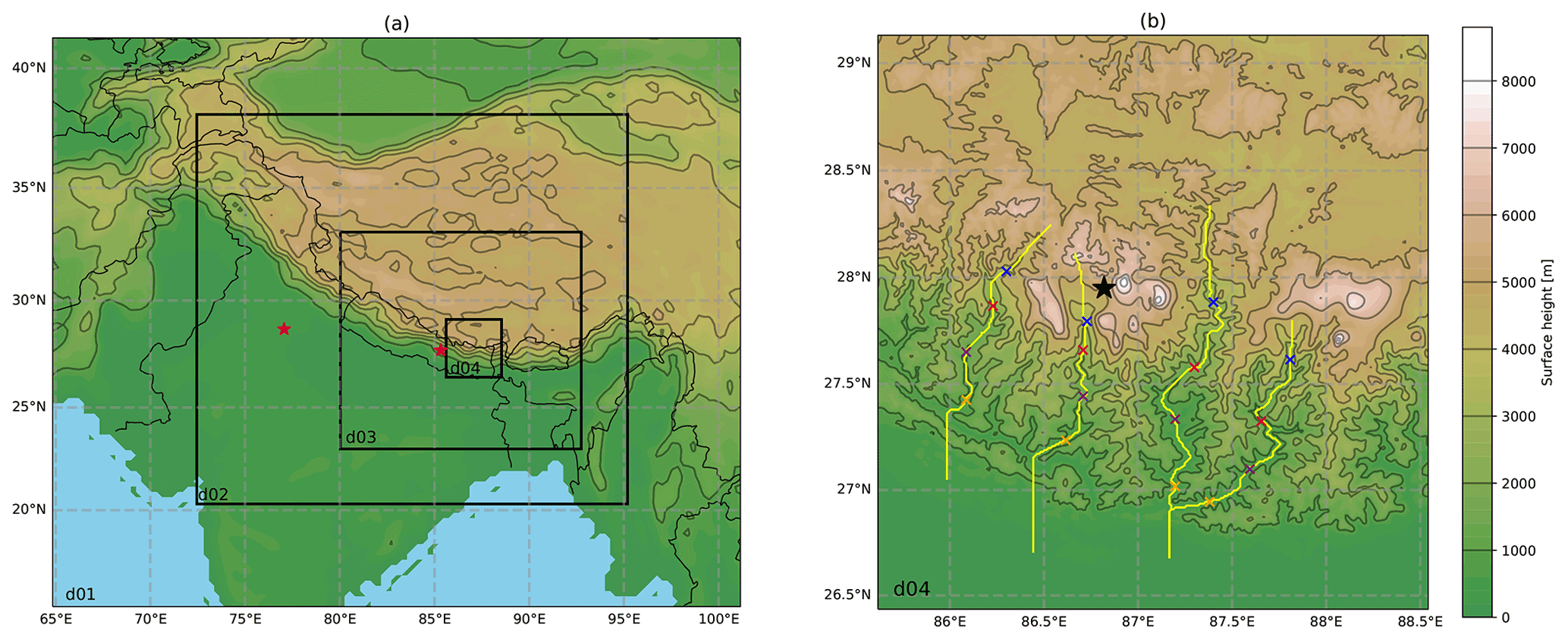
Figure 2 (a) Topography of the d01 domain and the inner domains, d02, d03 and d04, in the WRF simulation. Thin solid lines denote the country borders. Red stars denote the location of Kathmandu (the furthest east star) and New Delhi. (b) Topography of the d04 domain. Yellow lines present the valley centre lines used in the analysis. Valley names are listed from west to east: Gaurishankar, Khumbu, Makalu and Kanchanjunga. The black star indicates the location of the Nepal Climate Observatory – Pyramid (NCO-P) station. Coloured crosses denote locations along the valley centre lines that are referred to in the text and other figures.

Table 2 WRF-modelled values compared to near-surface observations in the Khumbu Valley, showing the mean bias error (MBE), mean absolute error (MAE) and root-mean-square error (RMSE) of the 2 m temperature and 5 m wind speed separately for daytime (06:00–18:00 LT) and night-time (18:00–06:00 LT).

The RMSE in the 2 m temperature ranges from 2.5 to 2.7 K for daytime (06:00–18:00 LT) and from 2.2 to 3.5 for night-time (18:00–06:00 LT) (Table 2). In the WRF simulation performed by Bonekamp et al. (2018), which has the same horizontal grid spacing and spin-up time as our simulation, the mean RMSE over all stations in Lang-tang Catchment is 8.0 K, which is notably larger than in our simulation. At NCO-P and Namche, the temperature in our simulation is underestimated for most of the simulation (the MBE is negative for both stations), but the simulated amplitude of the diurnal cycle is similar to the observed amplitude (Fig. S1b and d in the Supplement). At Lukla, the amplitude of the daily cycle of temperature is not captured well (MAE of 2.3 K), but the average temperature is closer to observations (daytime MBE of −0.5 K and night-time MBE of 2.3 K). At Lukla, the modelled maximum and minimum temperatures are around 2.5 K above and below the observation respectively. However, the timing of the diurnal cycle is well captured at all three stations (Fig. S1b, d and f in the Supplement).

The RMSE in 5 m wind speed ranges from 1.4 to 3.2 m s⁻¹ during daytime and from 0.5 to 2.9 m s⁻¹ during night-time (Table 2). In the WRF simulation performed by Bonekamp et al. (2018), the mean RMSE over all stations in the Lang-tang Catchment is 3.5 m s⁻¹, which is similar to the range that we compute. For both daytime and night-time, the RMSE in wind speed is lowest at Lukla and highest at NCO-P; moreover, the night-time RMSE is lower than the daytime value at each station. At each station, the diurnal cycle of the wind direction is modelled well, especially the daytime southerlies (Fig. S1a, c and e in the Supplement). At NCO-P, both the observed and modelled near-surface winds do not have a clear diurnal cycle with respect to speed (Fig. S1a in the Supplement); this is also seen in the skill scores (daytime MAE of 2.5 m s⁻¹ and night-time MAE of 2.4 m s⁻¹). At Namche, a clearer diurnal cycle is seen in both modelled and observed near-surface wind speeds (Fig. S1c in the Supplement). At Lukla, the observed wind speeds are less than 2 m s⁻¹ during the whole 4 d period, and the modelled wind speeds are notably larger and exhibit a clearer diurnal cycle (Fig. S1e in the Supplement) which leads to a higher MAE and MBE during daytime (MAE and MBE of 1.2 m s⁻¹) compared with night-time (MAE of 0.3 m s⁻¹ and MBE of 0.4 m s⁻¹). The weak observed winds may be due to sheltering by the nearby trees; thus, the Lukla AWS may not be representative of the area covered by the closest WRF grid box. However, overall, the modelled diurnal cycle of winds (with respect to both magnitude and direction) agrees reasonably well with the observations; hence, we conclude that the WRF simulation is sufficient for simulating the valley winds.

2.3 Diagnostics

2.3.1 Valley geometry

In this section, we define a number of diagnostics that quantify the topography and geometry of the valleys and, thus, enable us to quantitatively compare the four different valleys.

The valley centre lines (in yellow in Fig. 2b) were identified using a simple algorithm. The algorithm starts from the valley top, from a grid point chosen by the user, from where it finds the way down to the valley entrance by choosing the neighbouring grid point with the lowest surface height. This procedure continues over and over until the valley entrance is reached (determined by the user). The yellow lines in Fig. 2b were manually extended from the valley entrance to reach over the adjacent plain. In the case of the two westernmost valleys – the Gaurishankar and Khumbu valleys – the valley centre lines were extended due south over the perpendicular barrier from the valley entrance instead of continuing with the algorithm until the plain is reached. The daytime up-valley winds are connected to the plain by winds that propagate over this topographical barrier, so it is reasonable to follow this line in the analysis (discussed further in Sect. 4).

The ridgelines (not shown) were identified using a similar algorithm, with a small modification to the aforementioned technique. Now the algorithm chooses the neighbouring grid point that has the highest surface height but is additionally forced to propagate into the assumed direction of the ridge, chosen by the user based on the topography map. The ridgeline determination is a difficult task, as the valleys have, for example, a couple of “Eight-thousander”¹ around them. However, the use of these identified ridgelines allows us to approximately estimate the average depth of the valley atmosphere in these valleys.

The valley width is calculated at an elevation of 1000 m above the valley centre line. The width estimate is the distance between the west and east wall from the grid points where the elevation is above 1000 m compared with the valley centre line height. The west and east walls are found by moving in a direction perpendicular to the valley centre line. This value does not give an absolute value for the valley widths, but it does provide a comparable number for different parts of each valley, which was a more convenient approach to visualise the narrowing and widening of the valley topographies with the complex valley topographies with multiple side-valleys. The narrowing and widening of the valley topography can be important for the valley volume effect related to the along-valley winds. The elevation of 1000 m above the valley centre line was chosen based on the valley depths; most of the valleys have a minimum depth of 1000 m (valley topographies are described in detail in Sect. 3).

2.3.2 Along- and cross-valley wind components

As the valleys are not exactly north–south orientated at every point in the along-valley direction, the meridional and zonal winds in the model output can not be considered to be the along- and cross-valley wind components directly. The along- and cross-valley wind components are the wind components parallel and perpendicular to the valley centre line respectively (described in Sect. 2.3.1).

We use the vector ${\mathit{A}}_i=\mathit{x}(x_{i+\mathrm{3}}-x_{i-\mathrm{3}})+\mathit{y}(y_{i+\mathrm{3}}-y_{i-\mathrm{3}})$ to describe the local orientation of the valley at the ith grid point on the valley centre line. Here, (x_i,y_i) denote the coordinates of the ith grid point on the valley centre line in the inner model domain grid. Three grid points before and after the actual location are used to smooth out the sharpest turns in the valley centre line. Here, we write the horizontal wind in Cartesian coordinates, $\mathit{V}=\mathit{x}u+\mathit{y}v$, where u and v refer to the zonal and meridional wind components respectively. The along-valley wind component at the valley grid point i, AVW_i, is then calculated using Eq. (4):

$$\begin{array}{}\text{(4)}& {\mathrm{AVW}}_i={\displaystyle \frac{{\mathit{A}}_i}{\left|{\mathit{A}}_i\right|}}\cdot {\mathit{V}}_i={\displaystyle \frac{u_i\left(x_{i+\mathrm{3}}-x_{i-\mathrm{3}}\right)+v_i\left(y_{i+\mathrm{3}}-y_{i-\mathrm{3}}\right)}{\sqrt{{\left(x_{i+\mathrm{3}}-x_{i-\mathrm{3}}\right)}^{\mathrm{2}}+{\left(y_{i+\mathrm{3}}-y_{i-\mathrm{3}}\right)}^{\mathrm{2}}}}}.\end{array}$$

The cross-valley wind component is calculated using the same approach. Here, the cross-valley wind is perpendicular to the along-valley wind, but it is calculated at the slopes 5 to 10 grid points away from the valley centre line. The grid points on both slopes are selected to have the same elevation gain with respect to the valley centre line height and, thus, can differ regarding their horizontal distance from the centre line. The wind component describing the cross-valley winds at the slopes located around the ith grid point in the valley centre line is calculated using Eq. (5):

$$\begin{array}{}\text{(5)}& \begin{array}{rl}{\mathrm{CVW}}_i& =\left(\mathit{z}\times {\displaystyle \frac{{\mathit{A}}_i}{\left|{\mathit{A}}_i\right|}}\right)\cdot {\mathit{V}}_i\\ & ={\displaystyle \frac{-u_i\left(y_{i+\mathrm{3}}-y_{i-\mathrm{3}}\right)+v_i\left(x_{i+\mathrm{3}}-x_{i-\mathrm{3}}\right)}{\sqrt{{\left(x_{i+\mathrm{3}}-x_{i-\mathrm{3}}\right)}^{\mathrm{2}}+{\left(y_{i+\mathrm{3}}-y_{i-\mathrm{3}}\right)}^{\mathrm{2}}}}}.\end{array}\end{array}$$

3 Overview of the topographic characteristics of the four valleys

The four valleys considered in this study and their centre lines identified by the algorithm described in Sect. 2.3.1 are marked using yellow lines in Fig. 2b. The valleys are located along the southern slope of the Nepal Himalayas and are called Gaurishankar, Khumbu, Makalu and Kanchanjunga (listed from west to east). The valleys are roughly north–south orientated and are inclined towards the north, so the valleys face south. Figure 3 gives an overview of the topographic characteristics along each of the four valleys based on the diagnostics defined in Sect. 2.3.1. All of the valleys have a similar degree of valley narrowing (decrease in valley width) from the valley entrance towards the valley top (blue lines in Fig. 3). The Khumbu Valley is an exception, as the valley becomes broader (i.e. the valley width increases) from the along-valley grid point 40 (x axis in Fig. 3b), at the valley floor elevation of 3000 m, towards the valley top (along-valley grid point 0). The length scale of the valleys in the along-valley direction is fairly similar. Gaurishankar is the shortest valley at approximately 80 km, whereas Makalu is the longest valley with a horizontal length of approximately 120 km in the along-valley direction from the valley entrance to the valley top (distance along the valley centre line from the blue to yellow cross in Fig. 3).

The valleys can be roughly divided in two groups based on their topographic characteristics: the two westernmost valleys, Gaurishankar and Khumbu (Fig. 3a, b), and the two easternmost valleys, Makalu and Kanchanjunga (Fig. 3c, d). Makalu and Kanchanjunga have rather flat valley floors from the valley entrance into the valley, with less than a 1^∘ inclination (brown shading in Fig. 3c and d). After 60 grid points (approximately 60 km) into the valley, the valley floors start to incline towards the valley top. In Makalu Valley, the valley floor elevation increases from 500 to 4000 m a.s.l. (metres above sea level) from grid point 120 to grid point 30 with the slope varying between 0 and 6^∘. In Kanchanjunga Valley, the floor inclination ranges between 1 and 3^∘ in the top half of the valley, between grid points 20 and 60. In contrast, the Gaurishankar and Khumbu valleys both have a continuous increase in the inclination that increases from 2^∘ (along-valley grid points 80–100) to 5^∘ towards the valley top.

The valley depth (the difference between the ridge and valley centre line heights) is lowest in the Gaurishankar Valley. The valley depth is shown by the purple line in Fig. 3, with the values on the right y axes. In Gaurishankar, the valley depth reaches around 2500 m, whereas the valley depth in the other three valleys is larger (in the range of 3500–4000 m). In the portions of the Makalu and Kanchanjunga valleys where the valley floor is flat, the valley depth increases at a constant rate from the valley entrance towards the valley top. In the Kanchanjunga Valley, the approximately constant increase continues until the valley top. In the Gaurishankar and Khumbu valleys, the valley depth increases are not as gradual, but the valleys still get deeper from the valley entrance towards the valley top.

The valley entrances are significantly different between the valleys. The up to 1000 m high and 10 km wide topographic barrier in the along-valley direction lies perpendicular to the entrances of the Gaurishankar and Khumbu valleys (around grid point 120 in Fig. 3a and b). The barrier has an inclination of up to 10^∘ on both the northern and southern slopes of the barrier. The entrances into the Makalu and Kanchanjunga valleys are, in contrast, open without any such obstacles.

In summary, the two westernmost valleys (Gaurishankar and Khumbu; Fig. 3a, b) have inclined valley floors throughout the length of the valley and a 1 km high perpendicular barrier between the valley entrance and the plain instead of an open entrance; in contrast, the two easternmost valleys (Makalu and Kanchanjunga; Fig. 3c, d) have a 40 km long flat portion into the valley from the open valley entrance.

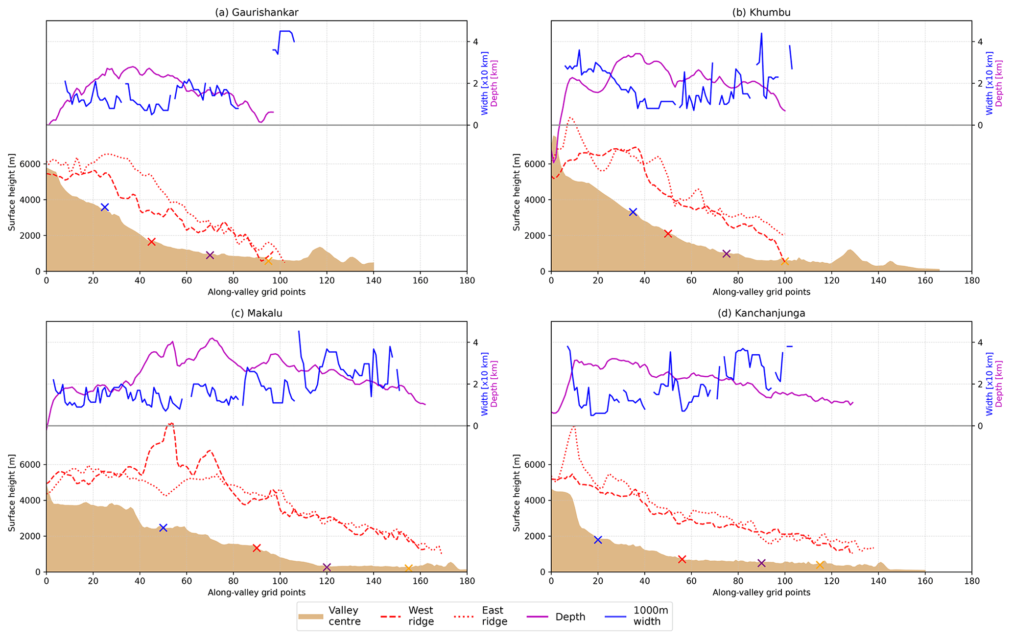
Figure 3 The height profiles (brown shading) of the valley centre lines (yellow lines in Fig. 2b) and the ridgelines (red dashed lines) correspond to the values on the left y axis. Cross-valley width at an elevation of 1000 m above the valley centre line is shown using the blue line. The valley depth is described as the height difference between the centre line and average of the ridgelines (shown in purple). The lines for width and depth correspond to the values on the right y axis. Each panel shows one valley: (a) Gaurishankar (most westerly valley), (b) Khumbu, (c) Makalu and (d) Kanchanjunga.

Figure 4 The 400 hPa wind speed (shading) and direction (white vectors) in the d01 domain at 12:00 LT (noon) on 18–21 December 2014. Black solid lines show the WRF simulation topography (m a.s.l.) with a contour interval of 1000 m. The red boxes mark the location of the inner domain d04.

4 Results

We first analysis the large-scale flow to ensure that it is consistent with the analysis in ERA5 (discussed in Sect. 2.1). Figure 4 shows the 400 hPa wind in the outer domain (d01) in the WRF simulation at 12:00 LT (noon) on 18–21 December 2014. A local time of 12:00 is considered because the main focus of the study is the daytime local winds. Overall, the 400 hPa wind speed and direction are similar between our simulation and the daily averages of ERA5 (Sect. 2.1). Most important for the study, the location and wind speed of the 400 hPa subtropical jet are very similar with respect to the high-resolution domain (d04) of our simulation.

The wind speed and direction above the valleys, particularly at ridge height, can influence the winds within the valleys (Whiteman and Doran, 1993; Solanki et al., 2019; Lai et al., 2021). The large-scale flow above the valleys changed from north-westerlies (18 December) to westerlies (19–21 December) as is seen in Fig. 4, where the red rectangles denote the location of the inner domain d04. The 400 hPa wind speed above the valleys was around 30–40 m s⁻¹ during the 18–20 December period (Fig. 4a, b, c), but it was weaker (20–30 m s⁻¹) on 21 December (Fig. 4d). The subtropical jet was located south-east of the inner domain (d04) location during the 18–20 December simulation period.

Daytime up-valley winds are found in all four valleys on each day of the simulation (Fig. 5); along-valley winds are discussed in detail in Sect. 4.1. The strongest daytime near-surface winds in the valleys are found around the valley centre lines (white dashed lines in Fig. 5) and have magnitudes of up to 10 m s⁻¹. The up-valley winds also spread into the smaller valleys branching off from the main valleys, but they are weaker than the up-valley winds in the main valleys.

The large-scale north-westerly winds at upper levels channel into the valleys, especially in the northernmost and thus highest parts of the Gaurishankar and Makalu valleys, on 18 December and are seen as strong down-valley near-surface winds during the day (Fig. 5a) and during the night between 17 and 18 December (Fig. S2a and c in the Supplement). Up to 25 m s⁻¹ near-surface down-valley winds are found in the tops of the valleys where the valley floors are at 4000–5000 m a.s.l. The tops of the Gaurishankar and Makalu valleys are favourable for large-scale north-westerlies to channel into the valley atmosphere. The north-westerlies penetrate into the valley atmosphere through the gaps and open south–north-orientated structures surrounding the top of the valley. The easternmost valley, Kanchanjunga, is an exception here because it is surrounded by sufficiently high ridges on the sides and at the valley top (Fig. 3d) that shelter the valley atmosphere from the large-scale flow channelling. Up to 25 m s⁻¹ near-surface winds are found on the ridges surrounding the Kanchanjunga Valley, but the near-surface winds stay below 10 m s⁻¹ and flow in the up-valley direction within the valley atmosphere. Due to the potential interruption of the thermally driven winds by the large-scale winds on 18 December and the fact that we want to focus on situations where there is little interaction with the large-scale flow, the analysis mostly concentrates on the 20–21 December period in the following sections.

The daytime valley winds propagate into the entrances of the two westernmost valleys (Gaurishankar and Khumbu) over the perpendicular topographic barrier from the plain (Figs. 2b; 3a, b). As we focus on the along-valley winds, it is sensible to extend the valley centre lines towards the plain over this barrier instead of following the topography towards the south-east (Fig. 2b). In this way, the structure of the flow in plain–valley interaction can be studied more successfully (cross-sections are discussed later in Sect. 4.2).

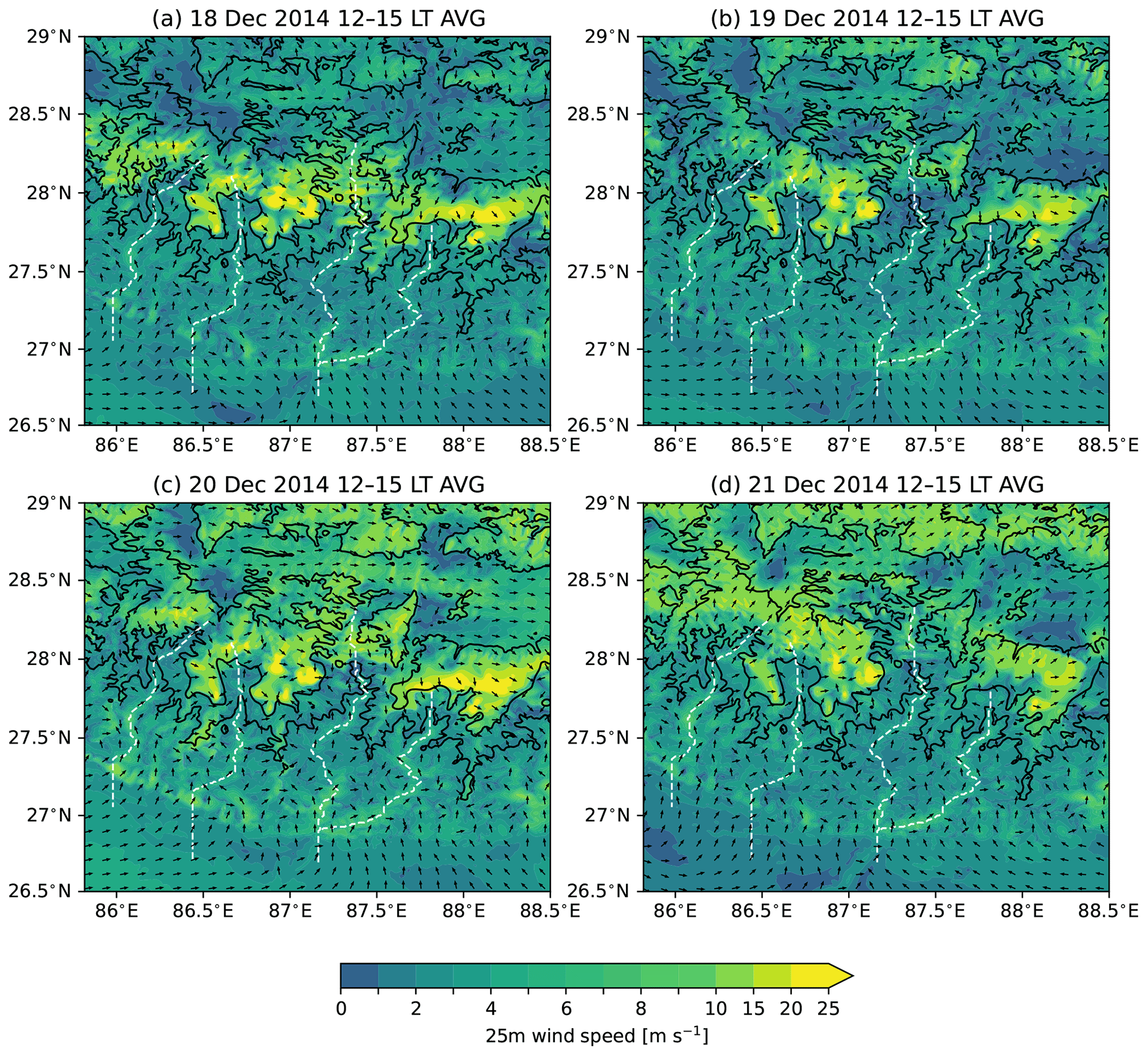
Figure 5 Wind speed (shading) and direction (black vectors) on the lowest vertical level (approximately 25 m above the surface) in the d04 domain on 18–21 December 2014. The wind is averaged over 12:00–15:00 LT for each day of the simulation. Black solid contours show the WRF simulation topography at 3000 and 5000 m a.s.l. Valley centre lines are shown by the white dashed lines.

Figure 6 Along-valley wind velocity in different parts of each of the four valleys (crosses of the same colours in Figs. 2 and 3) on the fourth model level (approximately 300 m above the surface). The numbers in the legends refer to the along-valley grid points as plotted on the x axes of Fig. 3. Positive values of wind velocity refer to up-valley winds. Local time is shown on the x axes. The data are plotted every 30 min. The same analysis with an extended y scale to show the along-valley wind velocities less than −5 m s⁻¹ is shown in the Supplement (Fig. S2).

4.1 Temporal evolution of the along-valley and cross-valley winds

The along-valley wind component is calculated based on Eq. (4) for four different parts of each valley. These locations are shown by crosses in Figs. 2b and 3, and the colours refer to the along-valley wind time series in Fig. 6. The along-valley wind component in Fig. 6 is the average of five grid points along the valley centre line around the crosses to describe the wind in a larger part of the valley, instead of only at one grid point. The four locations in the valleys represent the valley entrance (orange), two locations in the middle of the valley (purple and red) and the valley top (blue). The description of the along-valley winds is mostly based on the 20–21 December period, when the thermally driven winds were well defined in the valleys, but the 18–19 December period is also considered in the text.

The along-valley winds have a clear diurnal cycle with well-defined daytime up-valley winds and weak or absent nocturnal down-valley winds during 18–21 December (Fig. 6). During the study period the up-valley winds start developing around 09:00 LT, peak in magnitude around 15:00 LT and cease around 18:00 LT in all four valleys. The onset and offset of the daytime up-valley winds occur approximately 2 h after sunrise (06:50 LT) and 1 h after the sunset (17:12 LT) respectively. The along-valley winds at night are weak in all four valleys and generally remain in the up-valley direction (night-time is shown using shading in Fig. 6). On 18 December, the diurnal cycle is more interrupted than during the 19–21 December period, and the simulated night-time down-valley winds are caused by the channelling of the north-westerlies into the valleys. The high wind speeds caused by the channelling are shown in the Supplement (Fig. S2).

In Gaurishankar Valley, the daytime up-valley winds have maximum respective values of 5, 10, 5 and 4–6 m s⁻¹ at the four marked locations between 20 and 21 December, listed from the valley entrance to the valley top (Fig. 6a). During night-time, the winds are around 2 m s⁻¹ and are directed up-valley in the top half of the valley (grid points 25 and 45 in Fig. 6a), and they are less than 1 m s⁻¹ up- or down-valley in the lower half of the valley (grid points 70 and 95 in Fig. 6a). In the top of Gaurishankar Valley, the along-valley winds do not show a clear diurnal cycle except on the last day of the simulation. In other parts of the valley, the timing of the diurnal cycle is relatively similar on 18–21 December.

In Khumbu Valley, the daytime up-valley winds have maximum respective values of 3, 5, 4–5 and 2–3 m s⁻¹ at the four marked locations between 20 and 21 December, listed from the valley entrance to the valley top (Fig. 6b). During the simulation period, the wind speed is weakest at the valley top and strongest in the middle of the valley (Fig. S4c and d in the Supplement). During night-time, the along-valley winds remain mostly in the up-valley direction with magnitudes of less than 2 m s⁻¹ except at the valley top, where, on the night between 18 and 19 December, the along-valley wind is weak (<1 m s⁻¹) and in the down-valley direction (Fig. 6). The along-valley variation in the timing of the diurnal cycle is low in Khumbu Valley during the study period. Day-to-day variation in the along-valley winds is low, the along-valley wind speeds vary less than 2 m s⁻¹ in each part of the valley, and the onset and offset of the up-valley winds vary by less than 1 h during 18–21 December.

In Makalu Valley, the daytime up-valley winds have maximum respective values of 7–8, 6, 5 and 2–5 m s⁻¹ at the four marked locations between 20 and 21 December, listed from the valley entrance to the valley top (Fig. 6c). At the valley entrance, the night-time winds vary from 2.5 m s⁻¹ down-valley to 5 m s⁻¹ up-valley (yellow time series, grid point 155 in Fig. 6a). The along-valley winds do not have a clear repetitive diurnal cycle at the valley top except on the last day of the simulation. The timing of the diurnal cycle during 18–21 December varies among the different locations along the Makalu Valley. In the middle of the top half of the valley (red time series, grid point 90 in Fig. 6c), the onset, peak in magnitude, and offset of the up-valley winds are similar to those of the other valleys during the study period. At the valley entrance, the onset and peak in magnitude occur at the same time as in the other valleys, but the decay of the up-valley winds is slower; on 20 and 21 December, the along-valley wind component only changes to the down-valley direction at around 02:00–03:00 LT. In the middle of the valley (purple time series, grid point 120), the onset of the up-valley winds occurs at the same time as in the other valleys, but there are two maximums: the first around 15:00 LT and the second time around 18:00 LT. Thus, the decay of up-valley winds at this location is delayed by 3 h compared with the other valleys.

In Kanchanjunga Valley, the daytime up-valley winds have maximum respective values of 7–8, 6, 7 and 5 m s⁻¹ at the four marked locations between 20 and 21 December, listed from the valley entrance to the valley top (Fig. 6d). During night-time the along-valley winds remain in the up-valley direction, ranging from 1 to 5 m s⁻¹ during 20–21 December. The daytime up-valley winds only vary by 2–3 m s⁻¹ along the valley, and the onset and offset times are similar throughout the valley. The amplitude of the diurnal cycle is slightly larger in the middle of the valley than at either the valley entrance or the valley top. The up-valley winds extend all the way to the valley top on each day of the simulation. The decrease in the daytime up-valley winds is slower at the valley entrance compared with the other parts of the valley.

In all four valleys, the strongest up-valley winds occur at the entrances of the Makalu and Kanchanjunga valleys and 30 km into the Gaurishankar Valley (around along-valley grid point 70). In the Makalu and Kanchanjunga valleys, these strong valley entrance jets (Fig. S4e and g in the Supplement) could potentially be explained by the local strong temperature difference (discussed in detail in Sect. 4.2) between the valley and the plain, which would result in forcing of plain-to-valley winds.

In the 4 d simulation, the peak magnitude in winds in the Gaurishankar Valley is located near a narrow (in the cross-valley direction) part of the valley (as shown in Fig. S4a in the Supplement). The strong winds at this location can be explained by the Venturi effect (Whiteman, 2000). The local narrowing of the valley topography accelerates the wind speed through this gap, assuming a constant along-valley mass flux on both sides of the narrowing part. The wind speed above this location, 200 m higher than the model level that is shown in Fig. 6, is already reduced by half (not shown). The reduction in the wind speed with height is not as strong at the other locations in Gaurishankar Valley.

As an overview, excluding the parts of the valleys without persistent diurnal cycles in wind speed and the narrow gap channelling, the daytime up-valley winds are 2–3 m s⁻¹ stronger in the Makalu and Kanchanjunga valleys compared with the Gaurishankar and Khumbu valleys. The Kanchanjunga and Khumbu valleys have the most persistent diurnal cycle with respect to the up-valley winds in this 4 d simulation.

Figure 7 Cross-valley wind velocity in different parts of each of the four valleys (see Fig. 2b) on the lowest model level (approximately 25 m above the surface). Panels (a), (c), (e) and (g) are for grid points located on the western slope of the valleys, and panels (b), (d), (f) and (h) are for grid points on the eastern slopes. Local time is shown on the x axes. The cross-valley wind component on the western slope is multiplied by −1 to present both slopes such that positive values refer to an up-slope wind. The data are plotted every 30 min.

The cross-valley winds are shown in Fig. 7 in a similar manner to the along-valley wind components. However, whereas the along-valley winds were analysed in the centre of the valley, the cross-valley winds are analysed separately on both the east and west slopes of the valleys. The cross-valley wind component is considered here as a wind component perpendicular to the valley centre lines (introduced in Sect. 2.3.1) and, thus, perpendicular to the along-valley wind component directly above the valley centre line. Positive values for the cross-valley wind component on both slopes refer to up-slope winds. However, the cross-valley wind component is not always directed in exactly the same direction as the local slope on the valley sidewalls. This is because the sidewall slopes are not always perpendicular to the valley centre line.

A clear diurnal cycle of the up-slope cross-valley winds is only found in some parts of some valleys. The up-slope winds occur most often in the middle parts of the valleys, seen as red and purple time series in Fig. 7. At the locations with clear diurnal cycles, the daytime up-slope winds are less than 3 m s⁻¹ in magnitude and their vertical extent is less than 300 m (see Fig. S3 and S4 in the Supplement for vertical cross-sections of the wind components across the valleys).

A clear diurnal cycle of cross-valley winds on both the west and east slope at the same point is found only in the middle parts (red and purple time series) of the Makalu and Kanchanjunga valleys during the 19–21 December period (Fig. 7e, f, g, h). These locations refer to along-valley grid points 90 and 120 in Makalu and grid points 55 and 90 in Kanchanjunga. The up-slope winds start to develop right after sunrise at around 07:00 LT (sun rise 06:50 LT), peak in magnitude around noon and cease around 15:00 LT.

One of the analysed locations, the middle of the top half of Kanchanjunga (red time series in Fig. 7d), shows signs of a single circulation cell. Such a single circulation cell spans the whole cross-valley direction and can be identified if there are daytime up-slope winds at one slope and down-slope winds at the other slope (Fig. S3h in the Supplement).

Overall, from the WRF simulation, there is not strong evidence of well-defined thermally driven circulation in the cross-valley direction in the four valleys (Fig. S3 and S4 in the Supplement). However, the cross-valley winds shown in Fig. 7 are not the pure slope wind circulation, as the gradient of the slope elevation is not necessarily aligned perpendicularly to the valley centre line. Furthermore, the lowest three model levels at heights of 25, 90 and 190 m may not capture the thermally driven cross-valley circulation, due to the shallower nature of slope winds and the fact that night-time inversions may be below the lowest model level. Up to 10 m s⁻¹ wind speeds are simulated at the surface at higher elevations (i.e in the top parts of the Gaurishankar and Khumbu valleys; Fig. 7a, b, c, d). Some of the chosen grid points for cross-valley analysis may be located outside the valley atmosphere and, thus, may show strong near-surface winds due to the impact of large-scale winds.

4.2 Vertical structure of the along-valley winds and potential temperature

The vertical structure of the along-valley wind component and the potential temperature above the valley centre lines are plotted in Figs. 8 and 9 on 20 December at 09:00 and 15:00 LT respectively. The wind component parallel to the valley centre lines is plotted on each model level. The large spatial variability in the along-valley wind speed above the up-valley wind layers arises because winds above the valley atmosphere are stronger, and their direction is influenced by the large-scale flow and not the local topography. As this study concentrates on the daytime up-valley wind layer, the colour map for the wind shading is not optimal for wind speeds exceeding 10 m s⁻¹. The cross-sections show the whole length of the valley centre lines (yellow lines in Fig. 2b); thus, the far right-hand side of all the panels in Figs. 8 and 9 are the wind component and potential temperature above the plain.

In the morning (20 December at 09:00 LT – 2 h and 10 min after sunrise), the valley atmospheres are mainly characterised by weak up-valley winds (Fig. 8). The wind speed is mostly less than 2 m s⁻¹ in the Gaurishankar and Khumbu valleys, and the flow depth above the valley centre line is 500–1000 m. In the Makalu and Kanchanjunga valleys, the wind speed is up to 4 m s⁻¹, and the flow depth is 1000–1500 m above the valley centre lines. The up-valley winds exceeding 3 m s⁻¹ cover half of the along-valley distance in Kanchanjunga, whereas they are only found at the valley entrance in Makalu. Some parts of the valleys have weak (<2 m s⁻¹) near-surface down-valley winds which flow in shallow layers of less than 200 m. These weak down-valley winds are found in all of the valleys, but they only cover a minor share of the along-valley distance, and the up-valley winds are the dominant feature of the valley atmospheres, even in the morning.

In the morning (20 December at 09:00 LT), the potential temperature difference between the valley atmosphere and the plain is small in the layer where the up-valley winds flow (Fig. 8). This is seen as mostly horizontal isentropes between the valley atmosphere and the air above the plain (i.e. the lowest 1500 m from the ground). In all of the valleys, especially in their sloped parts, the isentropes turn towards the surface in a layer of 100–200 m, meaning that the valley floor is heated, even in the morning at 09:00 LT. In Kanchanjunga Valley (Fig. 8d), the isentropes already tilt towards the surface throughout the valley in the morning in a layer that is about 300 m deep, meaning that the valley atmosphere is warmer than the air above the plain. This is consistent with the stronger up-valley winds at this time in Kanchanjunga compared with the other valleys.

In the afternoon (20 December at 15:00 LT), the up-valley winds flow in the valley atmosphere all the way to the top of the valley (blue crosses in Fig. 9) in all four valleys. The up-valley wind speeds vary from 2 to 10 m s⁻¹ in the afternoon (described in detail in Sect. 4.1). The up-valley wind maxima are found around the same height in all of the valleys: around 200–300 m above the valley centre line. In the lower parts of the valleys (from the yellow crosses to purple crosses), the up-valley winds flow in a deeper layer compared with the upper parts (from red crosses to blue crosses). Figure 9 shows that the up-valley wind speed and depth are the most consistent along the valley in Kanchanjunga. The valley entrance jets are seen around grid points 140–160 in the Makalu Valley and around grid points 100–120 in the Kanchanjunga Valley (Fig. S3e and g in the Supplement). The narrow gap flow in the Gaurishankar Valley (discussed in Sect. 4.1), around the purple cross (grid point 70; Fig. S3a in the Supplement), is seen as a relatively small area of up-valley winds exceeding 10 m s⁻¹ (see also Fig. S4a in the Supplement). At the top of the Gaurishankar and Khumbu valleys, the depth of the up-valley wind layer decreases to a few hundred metres, although it still extends all the way to the top of the valleys (Fig. S4b and d in the Supplement). In the afternoon, all of the valley atmospheres are 3–5 K warmer in middle of the valley (purple crosses) compared with the same altitude above the plain (Fig. 9).

The plain-to-valley winds flow over the 1000 m high barrier at the entrances to the Gaurishankar and Khumbu valleys in a shallow layer of less than 500 m (grid points 110–130 in Gaurishankar and grid points 120–140 in Khumbu). The plain-to-valley winds basically stop between the leeward side of the barrier and the valley entrance (around grid point 110). In both the morning (Fig. 8a, b) and afternoon (Fig. 9a, b), the wind component towards the valleys decreases to 1 m s⁻¹ for the whole depth of the plain-to-valley wind layer. Along the leeward side of the barrier, between the plain and the Gaurishankar and Khumbu valleys, the isentropes descend and are parallel to the slope (Fig. 9a, b). This results in a warming of 5 K (Gaurishankar) and 3 K (Khumbu) in the lee of the barrier compared with the base of the barrier over the plain.

Figure 10 shows the potential temperature at 15:00 LT minus the potential temperature at 09:00 LT as a vertical cross-section above the valley centre lines on 20 and 21 December. The up to 1.5 K warming between 09:00 and 15:00 LT on 20 December and the cooling between 09:00 and 15:00 LT on 21 December at higher altitudes (>2000 m above the surface) most likely occur due to large-scale thermal advection. The valley atmospheres warm 4–6 K between 09:00 and 15:00 LT on 20 December. The surface-based warming extends to depths of less than 1000 m in the Gaurishankar and Khumbu valleys and to depths of less than 1500 m in the Makalu and Kanchanjunga valleys. The strongest warming between 09:00 and 15:00 LT is found in the near-surface layer (i.e. the closest 100–200 m to the surface). The warmed layer in the valley atmospheres decreases in magnitude and depth towards the top of the valleys. Where the valley floors start to incline strongly up towards the tops of the valleys is approximately where the warmed layer starts to become shallower. Unlike in the other three valleys, the valley floor in the Kanchanjunga Valley only starts to incline strongly close to the top of the valley, and the near-surface warming reaches further into the Kanchanjunga Valley compared with the other three valleys.

The qualitative difference between the spatial pattern of the thermal structure of the valley atmospheres on 20 and 21 December is small (Fig. 10a, c, e and g compared with Fig. 10b, d, f and h). The strongest warming is located around same parts of the valleys on both days. Considering that the daytime warming is also particularly affected by the large-scale weather above the valley atmosphere, the vertical extent of the strongest warming in the valley atmospheres is similar between the 2 d. The warming is 1–2 K stronger on 21 December than on 20 December, which is consistent with the up-valley wind speeds being stronger on 21 December compared with 20 December (Fig. 6).

Figure 11 shows the deviation of potential temperature at each along-valley grid point (y axis) on three model levels from the 2 d average of potential temperature during the 20–21 December period. Here, we define the amplitude of the diurnal cycle to be the difference between the maximum and minimum value of $\mathit{\theta }-\stackrel{\mathrm{‾}}{\mathit{\theta }}$ in Fig. 11.

Figures 10 and 11 show that the diurnal cycle of potential temperature reaches higher up in the valley atmosphere compared with over the plain. At the lowest model level (approximately 25 m above the surface; Fig. 11a, b, c, d), the diurnal cycle has a larger amplitude over the plain (up to 8 K) than in the valleys (4–6 K), but the amplitude decreases rapidly with height over the plain. At the height of approximately 450 m above the surface (model level 4; Fig. 11e, f, g, h), the amplitude of the diurnal cycle is less than 1 K above the plain, whereas the amplitude reaches up to 3 K in the Gaurishankar and Khumbu valleys and up to 5 K in the Makalu and Kanchanjunga valleys. The vertical extent of the warming is more evident in the cross-sections shown in Fig. 10, as the layer in which the surface-based warming exceeds 2 K between 09:00 and 15:00 LT is hundreds of metres deeper than above the valley.

In addition to the qualitative overview of the vertical structure of the along-valley winds and potential temperature field, a more detailed analysis of how the depth of the daytime up-valley wind layer and the depth of the warmed layer relate to each other is now considered. The depth of the up-valley wind layer is defined based on the model level at which the clear diurnal cycle vanishes in the along-valley wind time series (not shown, but one model level is shown in Fig. 6). Similarly, the vertical extent of the amplified diurnal cycle of potential temperature is based on the model level at which the daily range in potential temperature is the same as over the plain (not shown, but three model levels are shown in Fig. 11).

The depth of the up-valley wind layer and the vertical extent of the amplified diurnal cycle of potential temperature were defined based on the model level at which the clear diurnal cycle vanishes compared to the plain in the along-valley wind time series (not shown, but one model level is shown in Fig. 6) and in the amplitude of the diurnal cycle of potential temperature (not shown, but three model levels are shown in Fig. 11) respectively.

In the Gaurishankar and Khumbu valleys, the diurnal cycle of potential temperature and the up-valley winds are found in a layer that is 600–1200 m deep above the valley centre lines, whereas the corresponding depth is 1000–1500 m in Makalu and Kanchanjunga. In all of the valleys during the 4 d simulation, both the vertical extent of the diurnal cycle of potential temperature and the layer of up-valley winds is deepest in the lower parts of the valleys (yellow and purple crosses in Figs. 9 and 11). The up-valley wind layer is deepest in the portion of the Makalu (grid points 120–160) and Kanchanjunga (grid points 70–120) valleys with a flat valley floor, where the flow depth reach up to 1500 m, and shallowest at the top of the Gaurishankar (grid points 20–40) and Khumbu (grid points 30–50) valleys, where the flow depth is less than 600 m.

The vertical extent of the amplified diurnal cycle of temperature seems to correlate with the up-valley wind layer depth in the valleys: where the amplified diurnal cycle of temperature reaches higher, the daytime up-valley winds also reach higher. When the temperature in the valley atmosphere rises more compared with the air above the plain during daytime, using the hydrostatic law and ideal gas law combined, one obtains the qualitative result that pressure at the same height must be lower in the valley than over the plain. Thus, if the winds are driven by the pressure gradient force, the depth of the heated layer (i.e. in the valley atmosphere) would correlate with the depth of the daytime up-valley wind layer if pressure is horizontally homogeneous above the heated layer.

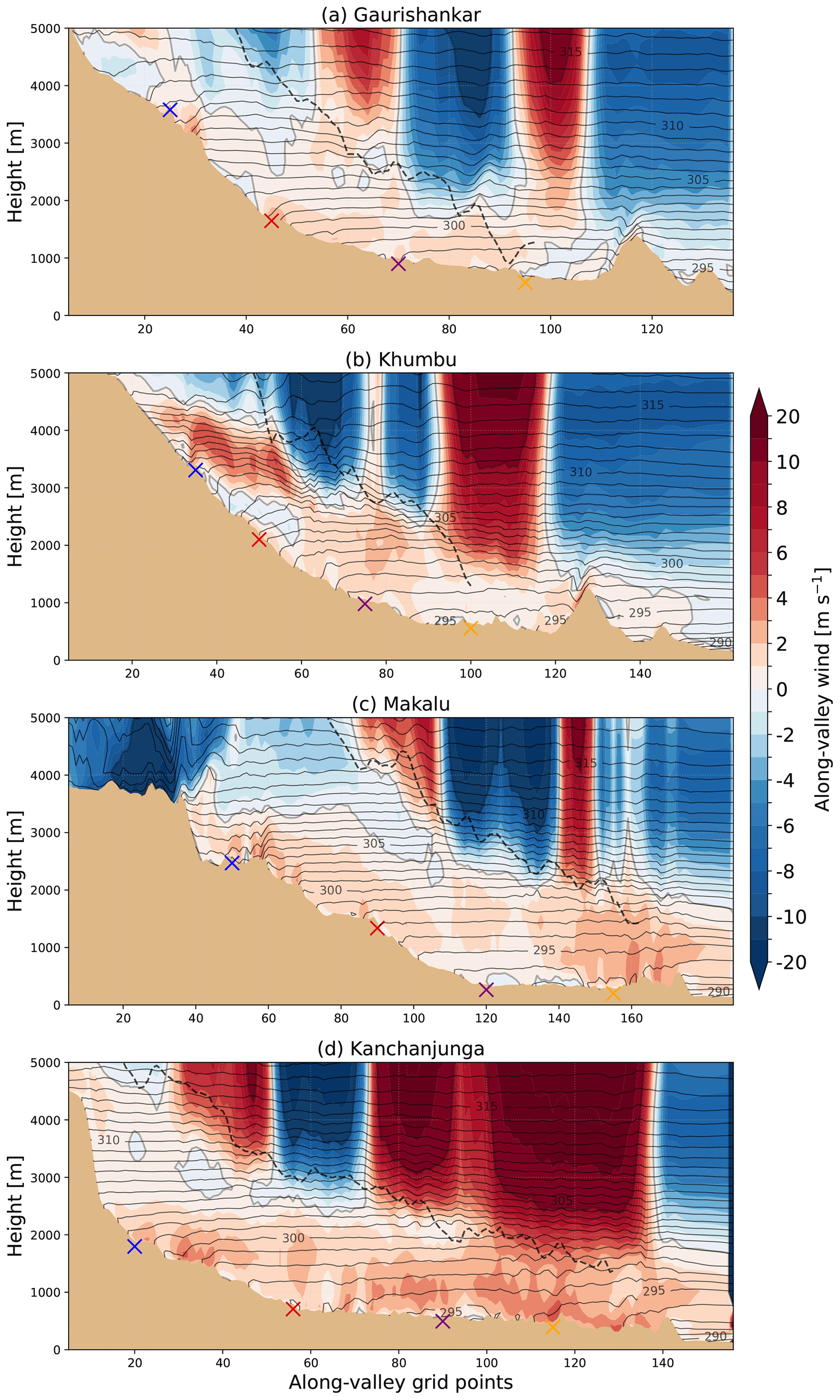
Figure 8 Vertical cross-section of potential temperature (grey contours) and the along-valley wind component (shading) above the valley centre lines (yellow lines in Fig. 2) on 20 December at 09:00 LT. Potential temperature is plotted with a contour interval of 1 K. Positive values for the along-valley wind refer to up-valley winds. The mean of the two ridge heights is shown by the black dashed lines.

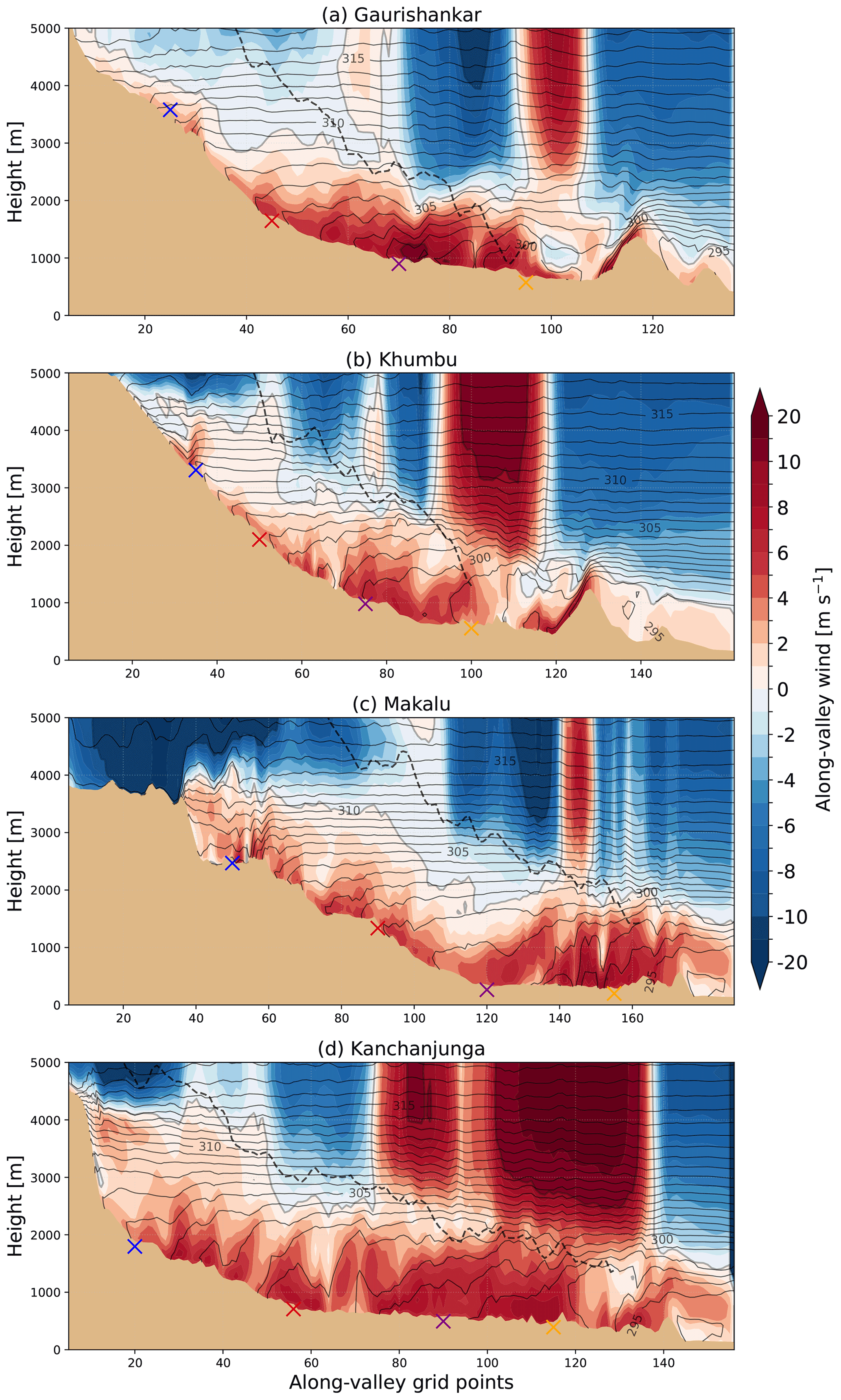
Figure 9 Vertical cross-section of potential temperature (grey contours) and the along-valley wind component (shading) above the valley centre lines (yellow lines in Fig. 2) on 20 December at 15:00 LT. Potential temperature is plotted with a contour interval of 1 K. Positive values for the along-valley wind refer to up-valley winds. The mean of the two ridge heights is shown by the black dashed lines.

Figure 10 Vertical cross-section of potential temperature change above the valley centre lines (yellow lines in Fig. 2b) between 09:00 and 15:00 LT on 20 December (a, c, e, g) and 21 December (b, d, f, h). Positive values indicate higher potential temperatures at 15:00 LT than at 09:00 LT.

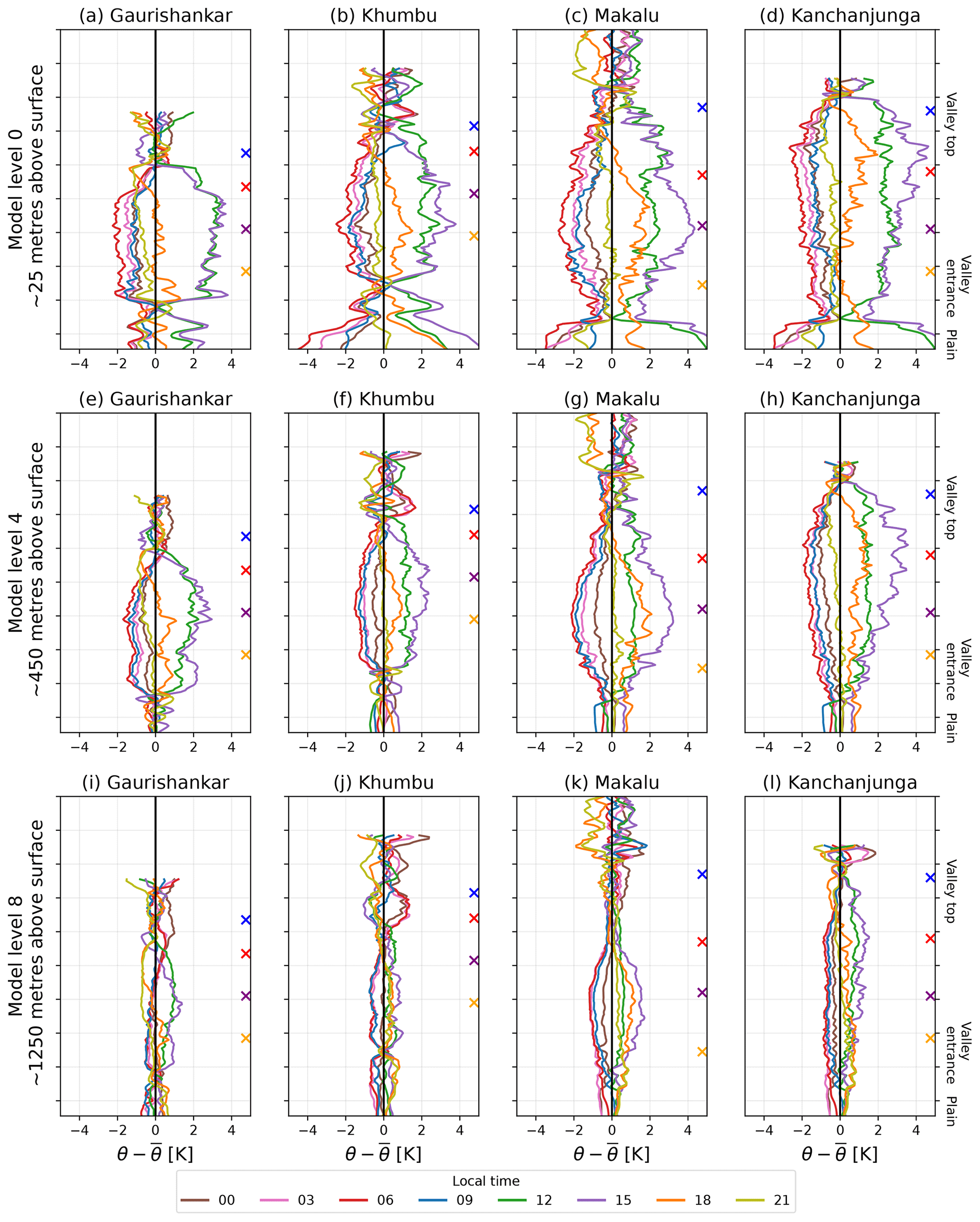
Figure 11 Diurnal variations in potential temperature in the valleys at model levels 0 (a–d), 4 (e–h) and 8 (i–l) during the last 2 d of the simulation (20–21 December 2014). The model levels refer to heights of (a–d) 25, (e–h) 450 and (i–l) 1250 m above the surface. The x axes show the deviation from the 2 d mean potential temperature of that model level in each grid point located on the valley centre line. The y axes are the grid points at the valley centre, and the crosses on the right-hand side of each figure denote the location of the grid points marked using the same colours in Figs. 2b and 3.

5 Discussion

We now attempt to understand the differences in the daytime up-valley winds during this 4 d period between the four valleys and along the individual valleys and to relate these differences to the differences in the valley topographies. To do this, we relate our results to previous studies that have used highly controlled idealised simulations to quantify the impact of valley geometry on valley winds. We also assume that, as all four valleys are under similar large-scale forcing, the differences in the along-valley winds are mainly due to differences in the valley topographies.

Two features that differ significantly in the valley topographies are the along-valley variation in the valley floor inclination and the topography of the valley entrances. As summarised in Sect. 3, the two westernmost valleys, Gaurishankar and Khumbu, have inclined valley floors throughout the length of the valley (1–2^∘ in the lower part of the valleys and 2–5^∘ in the upper part) and a 1 km high perpendicular barrier between the valley entrance and the plain. Makalu and Kanchanjunga, on the other hand, have a 40 km long almost flat portion close to the valley entrance and no barrier.

During the 4 d study period, the daytime up-valley winds are weaker and flow in a shallower layer in the parts of the valleys where the valley floor has a steep inclination (up to 5^∘). Wagner et al. (2015) studied the influence of valley geometry (e.g. floor inclination, width, depth and valley cross-section narrowing) on thermally driven flows using idealised numerical simulations. When they compared two straight valleys, one with a flat valley floor and the other with an inclination of 0.86^∘ in the valley floor, they found that the daytime up-valley wind speed increased by a factor of 3.0 in the valley with the inclined floor. Wagner et al. (2015) suggested that the increase in wind speed was due to both the reduction in the valley volume by 50 % and the additional buoyancy forcing from the slope wind effect. Our finding (that the strongest up-valley winds occur in the flatter parts of the valleys) appears to contradict the result of Wagner et al. (2015). However, in the four Himalayan valleys, the ridge height also increases along the valley, whereas the ridge height was constant along the valley in the idealised valleys that Wagner et al. (2015) studied. Therefore, in the Himalayan valleys, the steeply inclined valley floors do not necessarily lead to a reduced valley volume and enhanced topographic amplification factor along the valleys. In addition, the valley floors slope much more steeply in the Himalayan valleys compared with the valleys in Wagner et al. (2015). This may mean that the dominate driving mechanism of the up-valley winds differs in our simulations compared with the simulations of Wagner et al. (2015). Specifically, in steeply inclined valleys, the buoyancy mechanism that drives up-slope winds in classical mountain wind theories (Whiteman, 2000) may become more dominate than the valley-wind mechanism. The buoyancy mechanism drives shallower and weaker winds, such as the typical cross-valley slope winds, compared with the valley wind mechanisms. Shifting the dominant driving mechanism from the valley volume effect to the buoyancy mechanism, instead of combining their forcing, would explain the shallower and weaker up-valley winds in the steeply inclined parts of the four Himalayan valleys.

Instead of open valley entrances, the Gaurishankar and Khumbu valleys have a 1 km high barrier between the valleys and the plain. As discussed in Sect. 4.2, the daytime plain-to-valley winds cross this barrier in a shallow layer of a few hundred metres. In contrast, in the Makalu and Kanchanjunga valleys, the plain-to-valley winds flow in layers as deep as 1000–1500 m. The up-valley winds basically stop on the northern side of the barrier close to the valley entrances of Gaurishankar and Khumbu. The up-valley wind propagation into the valley could be significantly interrupted by the flow forced to flow over the 1 km high barrier. The flow characteristics over this barrier are similar to what Stull (1988) describes with respect to the down-slope wind storms associated with hydraulic jump. The strong and shallow flow over the barrier is followed by weaker horizontal winds on the leeward side after the barrier.

Bianchi et al. (2021) suggested that the daytime up-valley winds in the Khumbu Valley would transport aerosol precursors from the bottom of the valley to the free troposphere. During this transport, these gases are oxidised and, therefore, able to form new particles and influence the climate once they are in the free troposphere. They combined in situ aerosol observations and numerical model simulations with the high-resolution WRF model and the Lagrangian flexible particle dispersion mode (FLEXPART). They propose that other valleys on the southern slope of the Himalayas would also act as sources of free-tropospheric aerosol. We show that, regarding the daytime up-valley winds, the Khumbu Valley is not an exception compared to the other major valleys in this region. Based on the along-valley winds, aerosol and its precursors could be ventilated into the free troposphere from the other three valleys as well.

6 Conclusions

The local valley winds in the Nepal Himalayas during the 18–21 December period in 2014 were studied using a high-resolution WRF simulation. The horizontal grid spacing in the inner domain is 1 km, and the model is run with 61 vertical levels. A 12 h spin-up period is applied; hence, the first 12 h of the 5 d simulation (17 December from 06:00 to 18:00 LT) is excluded from the analysis.

Four major valleys are present in the innermost model domain, and the characteristics of the along-valley winds that develop in each of these valleys during this 4 d period were analysed and compared to each other. These Himalayan valleys have very different topographies compared with the much more extensively studied valleys in the European Alps and Rocky Mountains. Specifically, the floors of the Himalayan valleys studied here are steeply inclined and rise from less than 500 m a.s.l. to 4000–5000 m a.s.l. over a 100 km horizontal distance along the valley.

The simulation is evaluated using meteorological observations from three AWSs in the Khumbu Valley. Overall, the model manages to simulate the diurnal cycle of the winds that was evident in the observations. The along-valley wind characteristics in Khumbu Valley were found to be similar to what previous research has shown, with respect to both observational (Inoue, 1976; Ueno and Kayastha, 2001; Bollasina et al., 2002; Ueno et al., 2008; Bonasoni et al., 2010; Shea et al., 2015) and model-based studies (Potter et al., 2018, 2021).

Daytime up-valley winds are found in all four valleys during the simulated 4 d period. The night-time along-valley winds are weak and flow mostly in the up-valley direction. During large-scale north-westerlies (18 December), the daily cycle of along-valley winds is interrupted more compared with days with large-scale westerlies (20–21 December), especially at the tops of the Gaurishankar, Khumbu and Makalu valleys. The Kanchanjunga Valley is an exception among the valleys, as the daytime up-valley winds reach the top of the valley even during days with large-scale north-westerlies. The night-time down-valley winds are found more during the large-scale northerlies, which is most likely due to channelling of above-valley winds into the valley atmosphere.

During the simulated 4 d, the daytime up-valley winds vary between the valleys and their parts, with respect to both strength and flow depth. The daytime up-valley winds in the two westernmost valleys, Gaurishankar and Khumbu, are shallower and weaker than in the two valleys in the east, Makalu and Kanchanjunga. These two group of valleys can be separated by their topographical characteristics: the valleys in the west have a continuous inclination in the valley floor, and there is a 1 km high perpendicular mountain barrier between the valley entrance and the plain; the valleys in the east have a 40 (Makalu) and 60 km (Kanchanjunga) portion with a flat valley floor from the open valley entrance into the valley.

Steep inclination in the valley floor (2–5^∘) is associated with weaker and shallower up-valley winds compared with locations with a nearly flat valley floor (<1^∘ inclination). The perpendicular barrier at the valley entrance potentially interrupts the daytime plain-to-valley wind propagation, which is seen as weaker daytime up-valley winds at the valley entrance and potentially leads to weaker up-valley winds further up in the valley.

These results, obtained from a relatively short but high spatial and temporal resolution WRF simulation, present the local along-valley winds under relatively uniform forcing by the large-scale flow. Although the large-scale flow during the studied 4 d period is similar to the 40-year climatology, the results are subject to uncertainty, due to the short simulation period, and may not be valid under different or more time-variable large-scale forcing. This uncertainty could be resolved by the analysis of a longer model simulation covering differing large-scale flow regimes and different seasons. However, the methodology and the results of this study are a very useful starting point for a more long-term analysis of the local wind patterns in this understudied region of the Himalayas.