Meteorological modeling sensitivity to parameterizations and satellite-derived surface datasets during the 2017 Lake Michigan Ozone Study

High-resolution simulations were performed to assess the impact of different parameterization schemes, surface datasets, and analysis nudging on lower-tropospheric conditions near Lake Michigan. Simulations were performed where climatological or coarse-resolution surface datasets were replaced by high-resolution, real-time datasets depicting the lake surface temperatures (SSTs), green vegetation fraction (GVF), and soil moisture and temperature (SOIL). Comparison of two baseline simulations employing different parameterization schemes (referred to as AP-XM and YNT, respectively) showed that the AP-XM simulation produced more accurate analyses on the outermost 12 km resolution domain but that the YNT simulation was superior for higher-resolution nests. The diurnal evolution of the surface energy fluxes was similar in both simulations on the 12 km grid but differed greatly on the 1.3 km grid where the AP-XM simulation had a much smaller sensible heat flux during the daytime and a physically unrealistic ground heat flux. Switching to the YNT configuration led to more accurate 2 m temperature and 2 m water vapor mixing ratio analyses on the 1.3 km grid. Additional improvements occurred when satellite-derived surface datasets were incorporated into the modeling platform, with the SOIL dataset having the largest positive impact on temperature and water vapor. The GVF and SST datasets also produced more accurate temperature and water vapor analyses but had degradations in wind speed, especially when using the GVF dataset. The most accurate simulations were obtained when using the high-resolution SST and SOIL datasets and analysis nudging above 2 km a.g.l. (above ground level). These results demonstrate the value of using high-resolution satellite-derived surface datasets in model simulations.

1 Introduction

Locations along the Lake Michigan shoreline in the United States of America have a long history of recording surface ozone concentrations that exceed the levels set by the National Ambient Air Quality Standards (NAAQS), especially during the warm season (Stanier et al., 2021). Since the first ozone NAAQS was released in 1979, most lakeshore counties in the states bordering Lake Michigan (Wisconsin, Illinois, Indiana, and Michigan) have been designated as being in nonattainment for surface ozone in one or more of the subsequent NAAQS revisions. These states are required by the Clean Air Act to develop State Implementation Plans (SIPs) to demonstrate strategies to bring the affected areas into attainment and to mitigate the impacts of high-ozone concentrations. Large decreases in local emissions of ozone precursors such as nitrogen oxides and volatile organic compounds have steadily reduced the 1 and 8 h maximum ozone concentrations across the region in recent decades. However, the implementation of stricter ozone NAAQS means that additional air quality modeling assessments are necessary to help states demonstrate that they can reach attainment by the required statutory deadlines.

Urban and rural areas near Lake Michigan are susceptible to high-ozone events due to the complex interaction between synoptic and mesoscale circulation patterns, with large sources of industrial, transportation, and urban emissions along the southern end of the lake. High-ozone days are most common when synoptic-scale weather patterns characterized by weak southerly winds transport ozone and its precursors northward from their primary source regions over the Chicago and Milwaukee metropolitan areas and then interact with the mesoscale lake and land breeze circulations (Lyons and Olsson, 1973; Ragland and Samson, 1977; Lennartson and Schwartz, 2002). At night, the land breeze carries ozone precursors from land-based emissions sources over the lake, where they become confined within a shallow nocturnal boundary layer and are then converted into ozone after sunrise via photochemical processes (Dye et al., 1995). As the land surface warms during the day, a reversal of the mesoscale circulation leads to the formation of the lake breeze during the morning that transports the high-ozone air mass back onshore, with elevated ozone concentrations occurring across inland areas during midday and afternoon. On high-ozone days, the lowest ozone concentrations are often found in areas with high nitrogen oxide emissions, such as Chicago and northwestern Indiana, with the highest ozone levels located downwind in rural and suburban areas to the north of these urban and industrial locations (Foley et al., 2011; Cleary et al., 2015).

When synoptic-scale conditions are favorable for lake and land breeze formation, the horizontal temperature gradient between adjacent land and water areas influences the strength of the circulation pattern and the distance that the lake breeze penetrates inland during the daytime. Changes in the location of the lake breeze can have a profound impact on near-surface meteorology, the depth and vertical structure of the planetary boundary layer (PBL), and ozone concentrations along the Lake Michigan shoreline (Dye et al., 1995). Among other things, an accurate depiction of near-surface features in numerical weather prediction models requires an accurate specification of the lower boundary conditions at the land and water surface. For example, an accurate representation of land surface conditions (such as soil moisture, soil temperature, and green vegetation fraction) is necessary to correctly partition the surface net radiation into sensible, latent, and ground heat fluxes. This partitioning in turn impacts the growth and depth of the PBL and lower-tropospheric temperature, moisture, and wind profiles (Berg et al., 2014; Dirmeyer and Halder, 2016; Schwingshakl et al., 2017; Welty and Zeng, 2018). Soil moisture and vegetation fraction (or leaf area index) are especially important variables through their influence on the land–atmosphere coupling processes that link the surface hydrologic and atmospheric components of the Earth system (Santanello et al., 2018, 2019). Indeed, Huang et al. (2017) showed that the use of improved soil moisture and green vegetation fraction estimates in high-resolution simulations reduced biases in air temperatures and PBL heights over the Missouri Ozarks and had a large impact on biogenic isoprene emissions.

Given the important role that boundary layer meteorology and the land–lake breeze circulation have for ozone production and transport in the Lake Michigan region, it is critical to explore the ability of different parameterization schemes and surface datasets to improve the accuracy of near-surface meteorological and air quality simulations. For example, ozone production is highly sensitive to temperature and humidity (Bloomer et al., 2009; Camalier et al., 2007; Coates et al., 2016; Dawson et al., 2007; Jacob and Winner, 2009; Pusede et al., 2014), and the production and transport of ozone precursors such as nitrogen oxides and volatile organic compounds are also dependent on temperature and winds (Dye et al., 1995; Porter and Heald, 2019; Wang et al., 2022; Wiedinmyer et al., 2006). In this two-part study, we develop and assess the accuracy of a satellite-constrained modeling platform for the Midwestern United States that supports the needs of the Lake Michigan Air Directors Consortium (LADCO) as they conduct detailed air quality modeling assessments for the member states. The modeling platform uses high-resolution analyses of soil moisture, green vegetation fraction, and lake surface temperatures (SSTs) derived from satellite observations and an offline land surface model (LSM) to constrain the evolution of the lower boundary conditions during multi-week model simulations. In Part 1, we use the results from a large set of Weather Research and Forecasting (WRF) model simulations to assess the impact of the high-resolution surface datasets, different parameterization schemes, and analysis nudging on near-surface meteorological conditions and energy fluxes. We will show that a baseline model configuration employing default surface datasets produces better results for model simulations performed at 12 km horizontal grid spacing but that more accurate results are obtained at higher resolutions when the satellite-derived surface datasets and alternative parameterization schemes are used. In Part 2 of this study, we use meteorological analyses from two of the WRF model configurations as input to Community Multiscale Air Quality (CMAQ) model simulations to assess the impact of these model changes on ozone forecasts in the Lake Michigan region. The remainder of this paper is organized as follows: Sect. 2 contains a description of the model configurations and surface datasets. The results are presented in Sect. 3, with a discussion and conclusions provided in Sect. 4.

2 Methods

2.1 WRF model configurations

Version 3.8.1 of the WRF Preprocessing System (WPS) and WRF model (Powers et al., 2017) was used to perform simulations containing three one-way nested domains covering the contiguous United States, Midwestern United States, and Lake Michigan regions with 12, 4, and 1.3 km horizontal resolutions, respectively (Fig. 1). Each simulation contained 40 terrain-following vertical layers, with seven of the layers located below 2 km. The model top was set to 100 hPa. The 0.25^∘ resolution Global Forecast System Final (GFS-FNL) reanalyses, available at 6 h intervals, served as the initial and lateral boundary conditions (ICs and BCs) for the WRF model simulations. All simulations were run from 12 May–22 June 2017, with our evaluation focusing on the 22 May–22 June 2017 time period corresponding to the Lake Michigan Ozone Study field project (Stainer et al., 2021). Except for the two baseline simulations described below, all of the simulations were performed in daily increments using the standard WRF model restart files to allow for daily updates of high-resolution surface datasets using the WPS. The 40-category National Land Cover Database (NLCD) 2011 land use dataset (Jin et al., 2013) was used to determine the vegetation type and soil properties for each model grid point.

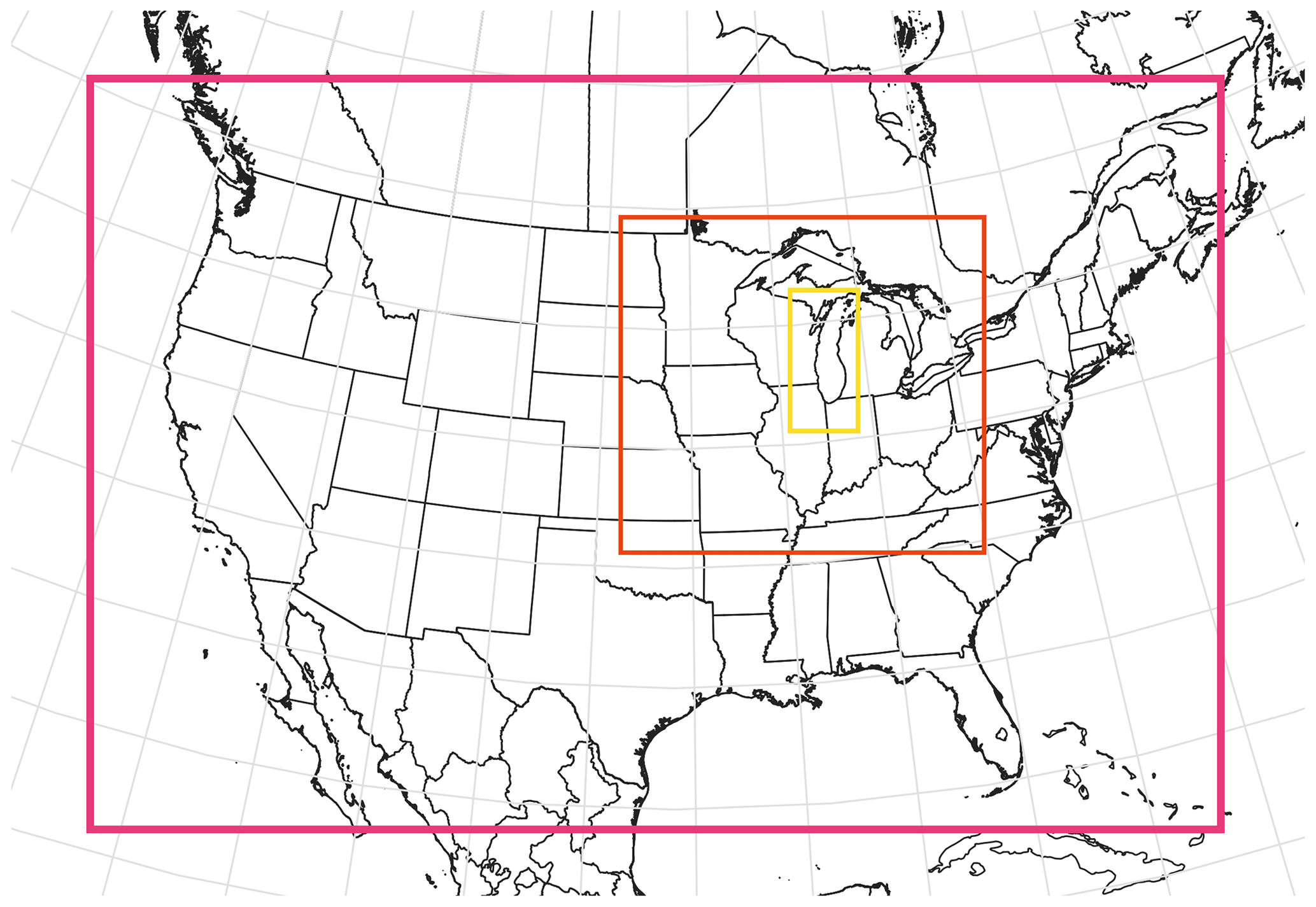
Figure 1 Map showing the geographic regions covered by the 12 km (red box), 4 km (orange box), and 1.3 km (yellow box) resolution domains used during the WRF model experiments.

Table 1 List showing the parameterization schemes, model initialization datasets, surface datasets, and nudging approaches used during each of the eight WRF model experiments. Acronyms are described in the text.

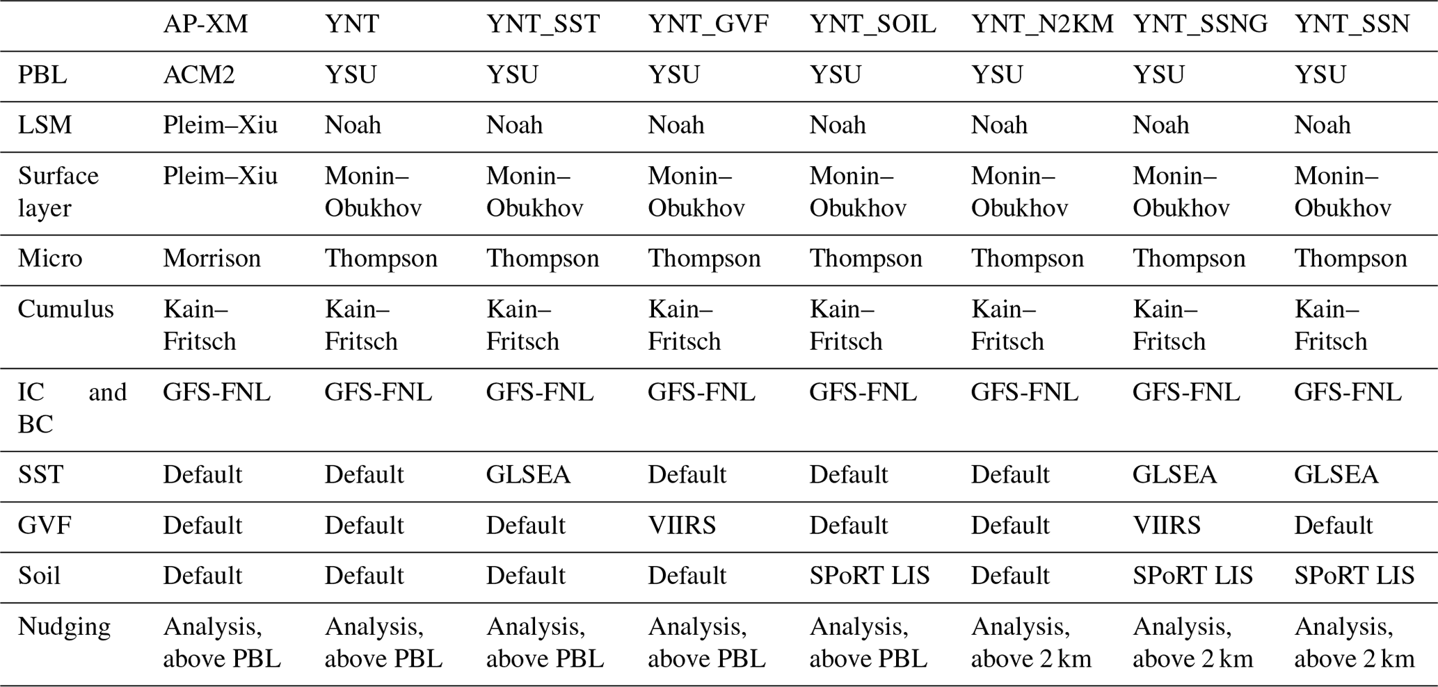
Eight model simulations were performed to assess the impact of different physics options and surface datasets on the model accuracy in the lower troposphere (Table 1). The first simulation, hereafter referred to as the AP-XM baseline configuration, employed the Morrison microphysics (Morrison et al., 2005), rapid radiative transfer model for general circulation models (RRTMG) longwave and shortwave radiation (Iacono et al., 2008; Mlawer et al., 1997), and ACM2 PBL (Pleim, 2007) parameterization schemes on all three domains, along with the Kain–Fritsch cumulus scheme (Kain, 2004) on the outer two domains. These schemes were chosen for the baseline configuration because they are often used in simulations performed at the U.S. Environmental Protection Agency (EPA). The ACM2 PBL scheme is a hybrid first-order closure scheme that attempts to capture both local and non-local fluxes (Pleim, 2007). When conditions are stable, only the local closure portion of the ACM2 scheme is used. Surface energy fluxes (sensible, latent, and ground) and changes in soil moisture and soil temperature were simulated using the Pleim–Xiu LSM (Gilliam and Pleim, 2010; Xiu and Pleim, 2001). In addition, analysis nudging was used to continuously adjust the temperature, water vapor, and winds above the PBL toward the 6 h GFS analyses (e.g., Borge et al., 2008; Campbell et al., 2019; Harkey and Holloway, 2013; Otte, 2008a, b; Otte et al., 2012; Pleim and Gilliam, 2009). Though additional procedures such as surface observation nudging and indirect soil moisture and soil temperature nudging (Pleim and Gilliam, 2009; Pleim and Xiu, 2003) are sometimes used to constrain the evolution of model simulations performed using the ACM2 scheme and Pleim–Xiu LSM, they are not employed during this study in order to maintain consistency with the other model simulations.

A second simulation was performed using the Yonsei University (YSU) PBL (Hong et al., 2006), Noah LSM (Chen and Dudhia, 2001; Ek et al., 2003), and Thompson microphysics (Thompson et al., 2008, 2016) schemes, which is hereafter referred to as the YNT configuration. Like the AP-XM simulation, this configuration employed the RRTMG longwave and shortwave radiation and Kain–Fritsch cumulus schemes on the outer two domains, along with grid nudging toward the GFS temperature, humidity, and wind analyses above the PBL. This particular set of schemes was chosen based on our previous studies, showing that they performed well during the warm season across the United States (e.g., Harkey and Holloway, 2013; Cintineo et al., 2014; Greenwald et al., 2016; Griffin et al., 2021; Henderson et al., 2021). Because there are dozens of parameterization schemes to choose from in the WRF model, we do not necessarily aim to find the best physics suite but instead to assess the potential of using other schemes to improve upon the performance of the baseline AP-XM configuration. The YSU PBL scheme is a first-order, non-local closure scheme that allows non-local mixing with explicit entrainment processes at the top of the PBL (Hong et al., 2006; Hong, 2010). The Noah LSM is a community model that has been widely used within the weather and climate modeling communities (Campbell et al., 2019). It contains four soil layers (0–10, 10–40, 40–100, and 100–200 cm depth), along with vegetation canopy, soil drainage, and runoff models that allow it to simulate surface hydrological and radiative processes. A realistic representation of land surface processes becomes increasingly important when moving towards higher model resolutions (e.g., Sutton et al., 2006; Case et al., 2008).

The remaining six simulations (Table 1) use the YNT configuration as their baseline. These simulations are designed to assess the impact of three high-resolution surface datasets and analysis nudging above 2 km (rather than above the PBL) on the model accuracy when used individually or in combination. In particular, three simulations were run where the standard climatological or coarse-resolution surface datasets were replaced by high-resolution, real-time datasets depicting lake surface temperatures, green vegetation fraction (GVF), and soil moisture and soil temperature across the study region. These surface datasets and the methods used to incorporate them into the WRF model simulations are described in the next section. Simulations employing these datasets are referred to as YNT_SST, YNT_GVF, and YNT_SOIL (where SOIL refers to soil moisture and temperature), respectively. Another experiment was performed in which analysis nudging was used above 2 km rather than above the PBL, which is referred to as the YNT_N2KM simulation. This change in nudging compared to the AP-XM and YNT baseline experiments was motivated by a modeling study by Odman et al. (2019), showing that the evolution of the nocturnal low-level jet across the Great Lakes region was more accurately simulated when nudging was withheld in the lower troposphere (e.g., below 2 km) when the PBL is shallow. Differences in the nocturnal low-level jet could affect the transport of ozone and its precursors from urban regions to Lake Michigan during the overnight hours. Finally, two combination simulations were performed in which the 2 km analysis nudging approach was used along with all three of the high-resolution surface datasets (YNT_SSNG) or only with the lake surface temperature and soil datasets (YNT_SSN). The latter simulation is included because it was found that this combination of surface datasets and analysis nudging generally led to the best results.

2.2 Surface datasets

2.2.1 Lake surface temperatures

Daily maps of the Great Lakes surface temperatures, with a horizontal resolution of ∼ 1.3 km, were obtained from the Great Lakes Surface Environmental Analysis (GLSEA) produced at the NOAA Great Lakes Environmental Research Laboratory (Schwab et al., 1992). The lake surface temperatures are estimated using clear-sky infrared brightness temperatures from the Advanced Very High Resolution Radiometer on board multiple polar-orbiting satellites. If a surface retrieval is not possible on a given day due to cloud cover, then a smoothing algorithm is applied to the previous analysis to maintain complete coverage. Only satellite observations are used to produce the daily lake surface temperature analyses, which have been shown by Schwab et al. (1992) to have a small bias and root mean square error (RMSE; 1–1.5 ^∘C) when compared to buoys. The daily GLSEA analyses were used to overwrite the simulated surface temperatures for Great Lakes grid points at 00:00 UTC on each day in the YNT_SST, YNT_SSN, and YNT_SSNG simulations using the WPS. Replacing the coarse-resolution (0.25^∘) GFS-FNL surface temperatures (Fig. 2a) with the GLSEA analyses (Fig. 2b) led to warmer lake temperatures near the shoreline, especially along the northern parts of Lake Michigan where temperatures were > 2 K warmer, and cooler temperatures across the rest of the lake, when averaged over the 22 May–22 June 2017 time period (Fig. 2c). This spatial pattern indicates that the finer horizontal resolution of the GLSEA dataset allows it to capture warmer temperatures in shallower waters near the shoreline while also depicting the cooler mid-lake temperatures due to the cooler-than-normal weather conditions that prevailed across the region in May (NCEI, 2017).

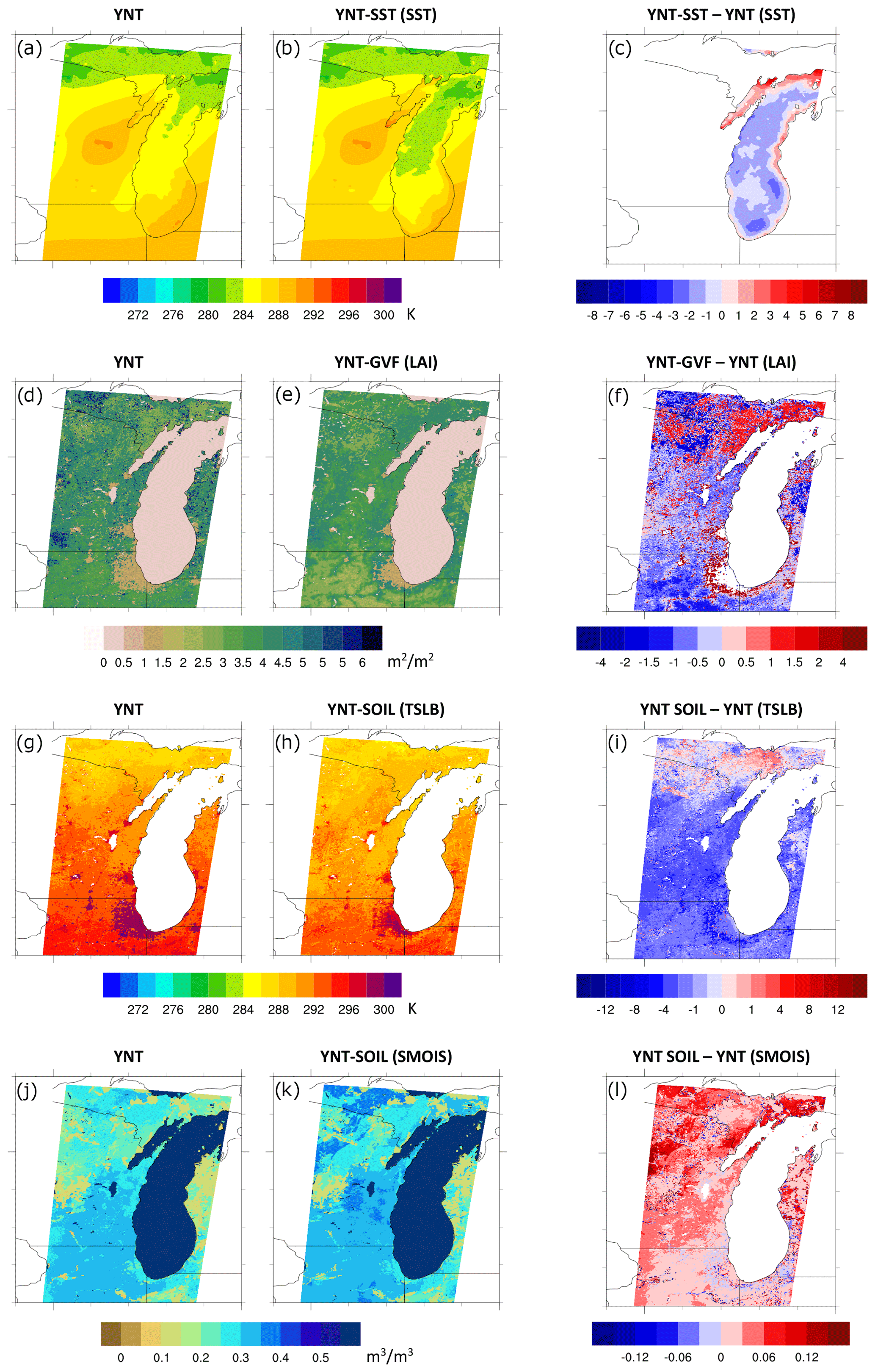
Figure 2 Average lake surface temperatures (K) from the (a) YNT and (b) YNT_SST simulations, with their differences shown in panel (c). Average leaf area index (m² m⁻²) from the (d) YNT and (e) YNT_GVF simulations, with their differences shown in panel (f). Average 0–10 cm soil temperatures (K) from the (g) YNT and (h) YNT_SOIL simulations, with their differences shown in panel (i). Average 0–10 cm soil moisture content (m³ m⁻³) from the (j) YNT and (k) YNT_SOIL simulations, with their differences shown in panel (l). The averages for each variable were computed using data valid at 00:00 UTC on each day during the 22 May–22 June 2017 time period.

2.2.2 VIIRS green vegetation fraction

GVF is the photosynthetically active fractional green vegetation cover within a grid cell, with higher values indicating more extensive actively transpiring vegetation. It is a key parameter in an LSM because vegetation representation is used to partition the incoming solar radiation into sensible, latent, and ground heat fluxes, where the latent heat flux is largely due to vegetation transpiration (e.g., Yin et al., 2016). Surface latent heat flux is sensitive to GVF because vegetation roots are able to access deeper soil moisture that would not otherwise be able to evaporate (Miller et al., 2006). For this study, we used daily global GVF derived using observations from the Visible Infrared Imaging Radiometer Suite (VIIRS; Vargas et al., 2015) instead of the default monthly climatology to constrain the evolution of vegetation in the YNT_GVF and YNT_SSNG simulations. The VIIRS GVF composite product is generated daily at 4 km resolution and available from the NOAA Comprehensive Large Array-data Stewardship System (CLASS). Ding and Zhu (2018) have shown that the VIIRS GVF product has smaller errors and bias than other satellite-derived GVF datasets because of reduced atmospheric influences, improved observing capabilities in high biomass regions, better representation of vegetation canopies, and reduced bidirectional reflection distribution function effects. The real-time daily GVF analyses were used to overwrite the default monthly climatological vegetation fraction data used by the WRF model at 00:00 UTC on each day. Using real-time, satellite-derived GVF instead of a monthly GVF climatology has been shown to improve the representation of the surface energy budget and subsequent model forecasts during the warm season (Case et al., 2014). In Fig. 2f, it is evident that use of the real-time GVF led to lower leaf area index (Fig. 2e; computed internally by the WRF model) across most of the domain compared to the climatological vegetation data (Fig. 2d), with the exception of some forested regions in the northern portion of the domain and bands of enhanced leaf area index surrounding metropolitan areas such as Chicago. The lower leaf area index in agricultural areas is consistent with delayed crop growth due to the cool spring weather, whereas the bands of higher leaf area index represent the impact of urban sprawl, since the climatological vegetation data shown in Fig. 2d were generated using satellite observations from the late 1980s and early 1990s (see Gutman et al., 1995).

2.2.3 SPoRT LIS soil moisture and temperature analyses

A customized version of the Land Information System (LIS; Kumar et al., 2006) run at the Short-term Prediction Research and Transition Center (SPoRT) was used to generate high-resolution soil moisture and soil temperature analyses. Version 3.6 of the Noah LSM (Chen and Dudhia, 2001) was run on a 1 km resolution domain covering the central and eastern United States and nearby portions of southern Canada. Required inputs to run the Noah LSM were obtained from hourly analyses of surface pressure, 2 m temperature, 2 m specific humidity, 10 m wind speed, and downwelling shortwave and longwave radiation from the North American Land Data Assimilation System Phase 2 (NLDAS-2; Xia et al., 2012). No observations were assimilated during the LIS runs. Quantitative precipitation estimates (QPEs) were obtained from the Multi-Radar/Multi-Sensor System (MRMS) gauge-adjusted radar product (Zhang et al., 2016), the Global Data Assimilation System (GDAS; Wang et al., 2013), and NLDAS-2. A simple blending methodology was used to incorporate the multiple sources of QPEs because an evaluation of the real-time SPoRT-LIS product (Case 2016; Case and Zavodsky 2018; Blankenship et al., 2018) and preliminary LIS experiments during this study revealed that the NLDAS-2 and MRMS precipitation products have a dry bias across the region. To reduce this bias, the precipitation forcing used the average of the highest two values of the MRMS, GDAS, and NLDAS-2 QPE datasets. Inspection of the blended precipitation product showed that the precipitation bias was reduced, while preserving small-scale spatial details in the MRMS QPE product. Daily VIIRS GVF composites were also used to constrain vegetation during the offline LIS-Noah simulation.

Following an initial spin-up of LIS using NLDAS-2 forcing data from 2012–2016 to remove the memory of the prescribed initial conditions, the final analysis from this run was used to restart the simulation on 1 January 2012 using NLDAS-2 atmospheric forcing data, VIIRS GVF, and the merged QPE product. Soil moisture and soil temperature analyses from this LIS simulation were then used to replace the corresponding variables in the YNT_SOIL, YNT_SSN, and YNT_SSNG simulations at 00:00 UTC on each day from 12 May–22 June 2017 using the WPS. Comparison of the 0–10 cm soil temperatures from the GFS (Fig. 2g) and LIS (Fig. 2h), averaged over the 22 May–22 June 2017 period, shows that the topsoil temperatures are noticeably cooler in the LIS data across most of the region, except for the northern parts of Wisconsin and Michigan. The cooler temperatures are most prominent in suburban regions, where the largest increases in GVF also occurred (Fig. 2f). For 0–10 cm soil moisture, the LIS analyses are generally wetter across the domain (Fig. 2l), with the largest increases across the forested regions of Wisconsin and Michigan. Deeper soil layers exhibited similar differences between the GFS-FNL and LIS datasets (not shown).

2.3 Evaluation methods

The accuracy of the WRF model simulations was assessed using hourly surface observations of temperature, humidity, and wind from the Meteorological Assimilation Data Ingest System (MADIS; https://madis.ncep.noaa.gov/, last access: 13 July 2023) during 22 May–22 June 2017. These observations were chosen because of their widespread availability and their important influence on surface chemistry processes. The model evaluations are performed on all three domains, using observations from stations located on the innermost domain surrounding Lake Michigan, which allows us to assess the behavior of each configuration as a function of spatial resolution using the same set of stations. Version 1.4 of the Atmospheric Model Evaluation Tool (AMET; Appel et al., 2011) from the EPA was used to collocate hourly observed and modeled values in a grid cell where a particular observation station was located and to calculate model performance statistics including bias and root mean square error.

3 Results

3.1 Assessment of AP-XM and YNT baseline experiments

This section contains a high-level assessment of the accuracy of the AP-XM and YNT baseline experiments on each domain, with a more detailed evaluation of all experiments on the 1.3 km resolution domain provided in Sect. 3.2. Figure 3 shows 2 m temperature, 2 m water vapor mixing ratio, and 10 m wind speed errors for each domain computed using hourly surface observations. The left column shows the bias for each variable and experiment, whereas the center and right columns show the percentage changes in RMSE for each experiment relative to the AP-XM and YNT baseline experiments, respectively. A negative (positive) value for a given variable and domain indicates that the RMSE for that experiment is smaller (larger) than the actual RMSE for the corresponding baseline experiment plotted in the gray box.

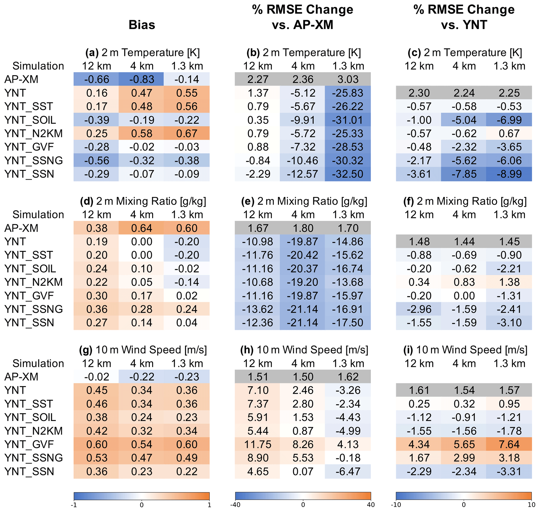
Figure 3 Summary statistics showing the (a) 2 m temperature bias for each experiment, along with the percentage change in the 2 m temperature root mean square error (RMSE) for a subset of experiments relative to the (b) AP-XM baseline and (c) YNT baseline experiments, respectively. Statistics for the 12, 4, and 1.3 km resolution domains were computed using hourly data from all stations located on the 1.3 km resolution domain during 22 May–22 June 2017. The actual RMSEs for the baseline experiments (gray boxes) are also shown. Blue (orange) shading indicates a negative (positive) bias for a given experiment in panel (a), whereas blue (orange) shading depicts a smaller (larger) RMSE in a given experiment relative to the AP-XM and YNT baseline experiments in panels (b) and (c). (d–f) Same as panels (a)–(c), except for showing statistics for the 2 m mixing ratio. (g–i) Same as panels (a)–(c), except for showing statistics for the 10 m wind speed.

Inspection of the YNT statistics reveals a consistent pattern in the RMSE, where the percentage changes for each variable either switch from positive to negative or become more strongly negative as the model resolution increases from 12 to 1.3 km. For temperature, the RMSE improves from being 1.37 % larger than the AP-XM on the 12 km domain to 25.83 % smaller on the 1.3 km domain (Fig. 3b). A similar pattern is present for 10 m wind speed, where the RMSE is 7.10 % larger on the 12 km domain but then steadily decreases so that the RMSE becomes 3.26 % smaller on the 1.3 km domain (Fig. 3h). The AP-XM simulation had a smaller wind speed bias on all three domains compared to the YNT baseline. For the 2 m mixing ratio (Fig. 3d, d), a positive bias on the 12 km domain increased at higher spatial resolutions for the AP-XM simulation but decreased and turned into a negative bias for the YNT simulation, which also exhibits a large reduction in the RMSE on all three domains. These results indicate that the AP-XM physics suite becomes less accurate at higher resolutions and that the YNT configuration provides superior performance on the 1.3 km domain when averaged across all stations. In the following sections, we will use the results from this domain to examine the impacts of the surface datasets and analysis nudging on the model accuracy with respect to the AP-XM and YNT baseline experiments.

3.2 YNT sensitivity experiments

3.2.1 The 2 m temperature evaluation

To examine regional differences in model performance, Fig. 4 shows the 2 m temperature bias and RMSE computed separately for each station using hourly observations from 22 May–22 June 2017. For the AP-XM simulation, there is a north–south gradient in the RMSE, with the largest errors across northern Illinois and Indiana (Fig. 4a). Stations near Lake Michigan have the smallest RMSE due to its moderating influence on local weather conditions. Similar to the RMSE, the smallest biases occurred in the northern part of the domain and along the eastern shoreline; however, biases along the western shoreline are larger and of comparable magnitude to those at inland locations across Wisconsin and Illinois. Overall, the AP-XM simulation had an RMSE of 3.03 K and a bias of −0.14 K when averaged across all stations (Fig. 3a–b). Switching to the YNT parameterization suite greatly reduced the RMSE by 25.83 % across the entire domain (Fig. 3b); however, the bias increased to 0.55 K (Fig. 3a). The largest RMSE reductions (up to 45 %) occurred in rural areas of northern Illinois, with similar RMSEs found across the entire domain (Fig. 4b). The larger positive temperature bias in the YNT baseline simulation is primarily due to larger errors in Wisconsin and within densely populated urban areas along the western Lake Michigan shoreline from Chicago to Milwaukee (Fig. 4f). A mixed pattern of larger and smaller biases occurred elsewhere across the domain.

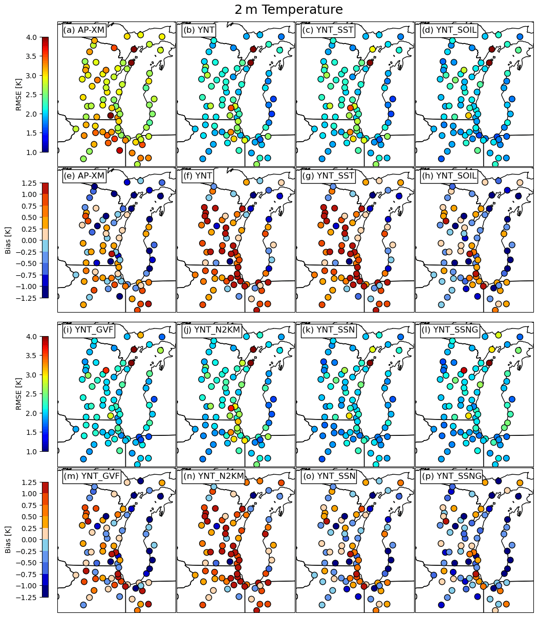
Figure 4 Maps showing the 2 m temperature (K), root mean square error (RMSE), and bias for each station on the 1.3 km domain computed using hourly data from 22 May–22 June 2017. Statistics for the EPA, YNT, YNT_SST, and YNT_SOIL experiments are shown in panels (a)–(h), whereas results for the YNT_GVF, YNT_N2KM, YNT_SSN, and YNT_SSNG experiments are shown in panels (i)–(p).

Inspection of the YNT sensitivity experiments shows that the smallest RMSEs occurred during the YNT_SOIL, YNT_SSN, and YNT_SSNG simulations, with the average RMSE reduced by 30.32 % to 32.5 % relative to the EPA baseline (Fig. 3b) and from 6.0 % to 9.0 % relative to the already greatly improved YNT baseline (Fig. 3c). On an individual basis, the high-resolution soil dataset (YNT_SOIL) had the largest positive impact at most stations (Fig. 4d), whereas slightly larger RMSEs were observed when using nudging (YNT_N2KM) (Fig. 4j). Comparison of the YNT_SSN and YNT_SSNG simulations (Fig. 4l, p) shows that inclusion of the VIIRS GVF dataset during the YNT_SSNG simulation led to slightly larger RMSE for stations near the lakeshore but similar or smaller errors for stations located further inland.

The bias pattern for the YNT simulations is more complex. Overall, the bias was largest (0.67 K) in the YNT_N2KM simulation, with the smallest biases occurring in the YNT_GVF (−0.03 K) and YNT_SSN (−0.09 K) simulations (Fig. 3a). Switching from the AP-XM to YNT baseline configurations led to larger biases across most of the domain, especially along the southwestern shoreline of Lake Michigan (Fig. 4e–f). The high-resolution SST dataset had a minimal impact on the biases (Fig. 4g), whereas they were smaller in the YNT_SOIL (Fig. 4h) and YNT_GVF (Fig. 4m) simulations relative to the YNT baseline. The use of these two land datasets, however, led to much larger negative biases along the eastern shoreline of Lake Michigan. When 2 km analysis nudging was used (YNT_N2KM), larger positive biases occurred from Chicago to Milwaukee, with smaller biases along the eastern shoreline (Fig. 4n). The increased RMSE and bias near the western shoreline compared to locations further inland during the YNT_N2KM simulation suggests that the modified nudging routine (applied to heights above 2 km instead of above the PBL) may not work well for areas near Lake Michigan due to the moderating influence of the lake on the PBL. Because the PBL tends to be more stable and shallower for locations over and near Lake Michigan due to the cooler surface temperatures, this means that confining analysis nudging to above 2 km limits its ability to constrain the evolution of the lower troposphere during the YNT_N2KM simulation. This behavior could also be due to deficiencies in the YNT configuration over complex urban–lake transition zones.

3.2.2 The 2 m water vapor evaluation

For the 2 m water vapor mixing ratio, switching to the YNT physics suite led to a reduction of nearly 15 % in the station-averaged RMSE during the YNT simulation relative to the AP-XM baseline (Fig. 3e), with additional incremental reductions occurring in all sensitivity experiments, except for YNT_N2KM (Fig. 3f). The lower RMSE in all of the YNT simulations is primarily due to the large reduction in bias (Fig. 3d). Whereas the AP-XM configuration had a large moist bias (0.60 g kg⁻¹), the YNT bias was much smaller and also became negative (−0.20 g kg⁻¹). The bias was further reduced during most of the sensitivity experiments, with only a slight increase during the YNT_SSNG simulation. Overall, the YNT_SSN simulation had the smallest RMSE and a bias close to zero when averaged across all of the stations.

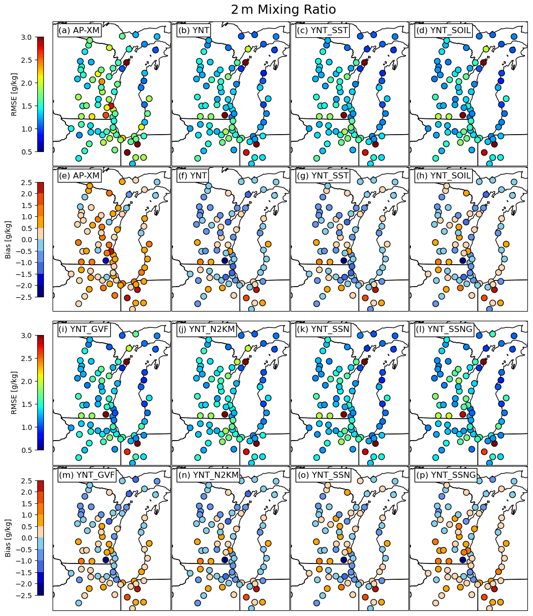
Figure 5 Same as Fig. 4, except for 2 m water vapor mixing ratio (g kg⁻¹).

Looking more closely at the individual stations (Fig. 5), it is evident that most of them have a positive (e.g., moist) bias when the AP-XM configuration is used (Fig. 5e). The largest biases are located in the southern portion of the domain, especially for stations near the lakeshore. In contrast, about two-thirds of the stations exhibit a negative bias during the YNT simulation (Fig. 5f). The spatial pattern of the biases is similar during all of the YNT sensitivity experiments; however, their magnitudes are generally smaller, which is consistent with the overall statistics (Fig. 3d). For RMSE, the largest errors in the AP-XM simulation occur primarily along the southern end of Lake Michigan, with generally smaller errors in the northern half of the domain (Fig. 5a). The RMSE during the YNT simulation is smaller at most locations, especially along the shoreline, though a few stations near the western shoreline have larger errors (Fig. 5b). The use of the SOIL and GVF datasets reduced the errors at these nearshore locations (Fig. 5d, i), with the smallest errors at most stations occurring during the combination experiments (YNT_SSN and YNT_SSNG). As was the case with 2 m temperature, the most accurate 2 m water vapor analyses were obtained during the YNT_SSN simulation.

3.2.3 The 10 m wind speed evaluation

Compared to the temperature and water vapor fields, changes to the 10 m wind speed statistics were much more modest during the YNT simulations. Switching from the AP-XM configuration to the YNT configuration led to a 3.26 % reduction in the RMSE but a larger bias that also changed sign from negative to positive (Fig. 3g). For the YNT experiments, the average RMSE was slightly smaller during the YNT_SOIL and YNT_N2KM simulations (−1.21 % and −1.78 %, respectively) but slightly larger (0.95 %) during the YNT_SST simulation compared to the YNT baseline (Fig. 3i). The use of the GVF surface dataset led to a 7.64 % increase in the RMSE during the YNT_GVF simulation, primarily due to a larger wind speed bias. Overall, the most accurate wind speed analyses were achieved during the YNT_SSN simulation, with an RMSE reduction of 6.47 % across all stations.

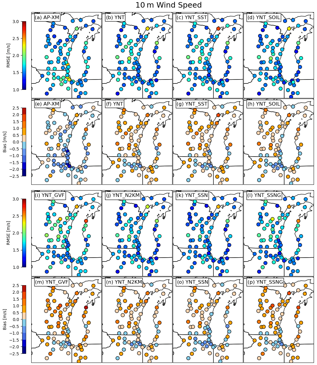
Figure 6 Same as Fig. 4, except for 10 m wind speed (m s⁻¹).

Spatially, there is a latitudinal gradient in wind speed errors during the AP-XM simulation. The largest RMSEs are located across the southern part of the domain (Fig. 6a), with mostly negative wind speed biases (up to 2 m s⁻¹) in the same region transitioning to a mix of negative and positive biases in northern Wisconsin and Michigan (Fig. 6e). The RMSE and bias were much smaller for stations around the southern shoreline of Lake Michigan during the YNT simulation; however, slightly larger RMSEs are present across inland locations in the northern part of the domain (Fig. 6b). A similar spatial pattern of changes relative to the AP-XM baseline occurred during the YNT sensitivity experiments, though the errors are generally larger during the YNT_GVF simulation (Fig. 6i, m) and smaller during the YNT_SOIL (Fig. 6d, h) and YNT_N2KM (Fig. 6j, n) simulations. The poor performance of the YNT_GVF and YNT_SSNG simulations is primarily due to larger errors across inland areas of Wisconsin, where there are large positive wind speed biases (Fig. 6m, p), with similar errors elsewhere in the domain.

3.2.4 Diurnal error characteristics

Figure 7 shows the diurnal evolution of RMSE and bias for 2 m temperature, 2 m water vapor mixing ratio, and 10 m wind speed at hourly intervals starting at 19:00 local standard time (LST). The time series were computed by averaging over data from all stations on the 1.3 km domain. Overall, it is apparent that the AP-XM simulation contains very different diurnal error patterns than the YNT simulations. For example, the 2 m temperature bias exhibits a prominent diurnal cycle (Fig. 7b) characterized by large positive and warm (negative and cool) biases during the night (day), resulting in an overall damping of the diurnal temperature cycle. The warm biases exceed 2.0 K during most of the night (22:00–03:00 LST), and the cold biases are < −2 K for several hours during the daytime (09:00–13:00 LST). These results indicate that the small temperature bias in the summary statistics for the AP-XM simulation (Fig. 3a) is misleading because it obscures the presence of substantial biases of opposite signs during the day and night. The RMSE is also much larger during the AP-XM simulation (Fig. 7a), with local maxima of 3.5 K at 11:00 and 23:00 LST, respectively, corresponding to peaks in the temperature biases. Switching to the YNT baseline greatly reduces the temperature RMSE, and the bias time series is no longer characterized by the highly amplified diurnal pattern seen in the AP-XM simulation. Examination of the YNT sensitivity experiments shows similar error patterns to the YNT baseline. The largest differences occur at night when the use of the GVF and SOIL datasets leads to smaller biases. In contrast, confining the analysis nudging to above 2 km a.g.l. (above ground level; YNT_N2KM) slightly increases the RMSE and bias during the nighttime relative to the YNT baseline.

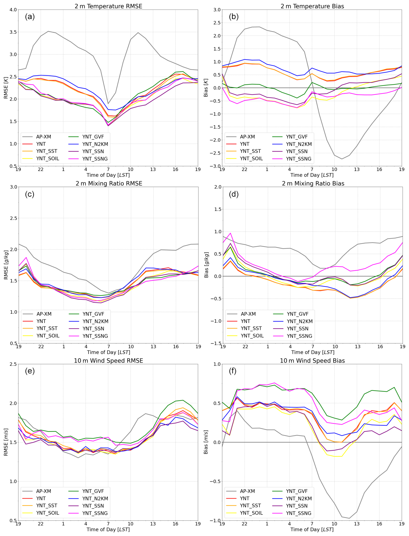
Figure 7 Time series showing the diurnal evolution of (a–b) 2 m temperature (K), root mean square error (RMSE), and bias, (c–d) 2 m water vapor mixing ratio (g kg⁻¹), RMSE, and bias, and (e–f) 10 m wind speed (m s⁻¹), RMSE, and bias at hourly intervals starting at 19:00 LST. Errors were computed for each model simulation using observations from all stations located on the 1.3 km resolution domain during 22 May–22 June 2017.

For water vapor, the AP-XM simulation again exhibits a larger bias and RMSE than the other simulations (Fig. 7c, d). It has a large moist bias that ranges from 0.2 g kg⁻¹ shortly after sunrise to 0.9 g kg⁻¹ near 19:00 LST, before decreasing to a relatively stable bias of 0.6 g kg⁻¹ during the night. The RMSE is smaller in the YNT baseline simulation, with a dry bias evident for all but the evening hours (19:00–22:00 LST). As is the case for temperature, the RMSE is smallest during the late-night hours and then steadily increases during the day before reaching its maximum in the evening. All of the YNT sensitivity experiments have similar RMSE and bias patterns to the YNT baseline, with the smallest (largest) spread between simulations occurring during the nighttime (daytime) hours, possibly due to differences in the PBL depth and surface energy balance (see Fig. 8). Comparison of the 10 m wind speed time series reveals that the AP-XM simulation has the smallest bias (∼ 0.15 m s⁻¹) during the night but that the wind speeds are weaker than observed during the daytime, with the largest biases (−0.95 m s⁻¹) occurring at noon (Fig. 7f). This diurnal pattern in the AP-XM simulation, characterized by winds that are too strong (weak) during the night (day), stands in contrast to the mostly positive biases in the YNT simulations. The biases are tightly clustered in all of the YNT experiments during the nighttime hours (22:00–07:00 LST), with the exception of the two simulations employing the GVF dataset (YNT_GVF and YNT_SSNG) that are characterized by persistently larger positive biases. These two simulations also have the largest RMSE (Fig. 7e). Further research is necessary to determine why the incorporation of the high-resolution GVF dataset leads to larger surface wind speed errors.

3.2.5 Surface energy budget considerations

Near-surface atmospheric conditions can be strongly impacted by the partitioning of net surface radiation into sensible, latent, and ground heat fluxes (Santanello et al., 2018). To examine this more closely, Fig. 8 shows a time series depicting the average diurnal evolution of the PBL height, net surface radiation, and sensible, latent, and ground heat fluxes during 22 May–22 June 2017 computed using data from stations on the 1.3 km domain to maintain consistency with earlier results. Because in situ flux and PBL height observations are not available across the entire domain, the aim is not to examine the accuracy of the simulated surface energy fluxes and PBL height but rather to use these variables to help explain differences in the near-surface temperature, water vapor, and wind speed errors in the model simulations. All of the variables were obtained directly from the WRF output files. The net surface radiation is defined as the sum of the upward and downward shortwave and longwave radiation fluxes at the surface.

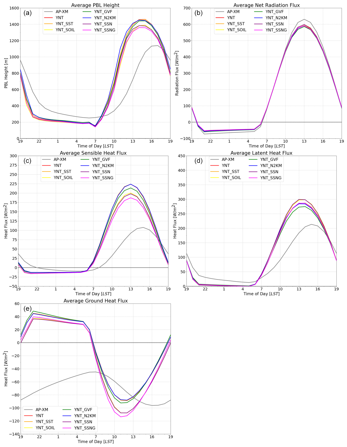
Figure 8 Time series showing the diurnal evolution of the (a) planetary boundary layer height (m), (b) net radiation (W m⁻²), (c) sensible heat flux (W m⁻²), (d) latent heat flux (W m⁻²), and (e) ground heat flux (W m⁻²) at hourly intervals starting at 19:00 LST, averaged over all stations on the 1.3 km domain during 22 May–22 June 2017. Results are shown individually for each of the model simulations.

Inspection of Fig. 8 reveals large differences between the AP-XM and YNT simulations. The PBL is ∼ 50–150 m deeper in the AP-XM simulation during the nighttime but then becomes much shallower than the YNT simulations from mid-morning through the afternoon (10:00–16:00 LST), with the daytime maximum in PBL height occurring ∼ 2 h later (Fig. 8a). The AP-XM simulation is also characterized by a smoother and less amplified diurnal evolution. For the YNT simulations, the PBL heights are tightly clustered during the night (21:00–07:00 LST) but begin to diverge during the morning and reach their largest differences during the afternoon. In particular, simulations employing the high-resolution soil moisture analyses (YNT_SOIL, YNT_SSN, and YNT_SSNG) have average PBL heights that are ∼ 100 m lower than the other YNT simulations. These three simulations also have slightly lower sensible heat flux (Fig. 8c) and higher latent heat flux during the afternoon (Fig. 8d), which is consistent with the wetter and cooler topsoil layer in the SPoRT LIS analyses (Fig. 2g–l) and cooler 2 m temperatures (Figs. 3a, 7b). Using the SST and GVF datasets and confining analysis nudging to above 2 km had minimal impact on the PBL heights in the YNT_SST, YNT_GVF, and YNT_N2KM simulations; however, sensible and latent heat fluxes are slightly smaller during the afternoon in the YNT_GVF simulation.

Comparison of the AP-XM and YNT simulations also reveals large differences in the surface energy flux time series. For example, the AP-XM simulation has much smaller sensible heat flux during the daytime (Fig. 8c), and the latent heat flux remains relatively large during the night (Fig. 8d). Though the AP-XM and YNT simulations produce similar magnitudes of latent heat flux during the day, the afternoon maximum is delayed by 2 h in the AP-XM simulation. The combination of a shallower PBL during the day (Fig. 8a) and higher latent heat flux at night likely contributes to the persistently large moist bias in the 10 m water vapor mixing ratio (Figs. 3d, 7d) during the AP-XM simulation. Another noteworthy feature of the AP-XM simulation is that the ground heat flux remains negative at all times. This unphysical behavior stands in sharp contrast to the more realistic evolution during the YNT simulations, where the positive (negative) ground heat flux during the night (day) indicates that heat is being transferred from (toward) the ground toward (from) the atmosphere due to cooler (warmer) surface temperatures. These results indicate that the poor performance of the AP-XM simulation on the 1.3 km domain, when assessed using near-surface moisture, temperature, and wind observations, is likely due to the presence of vastly different and sometimes unphysical surface energy fluxes.

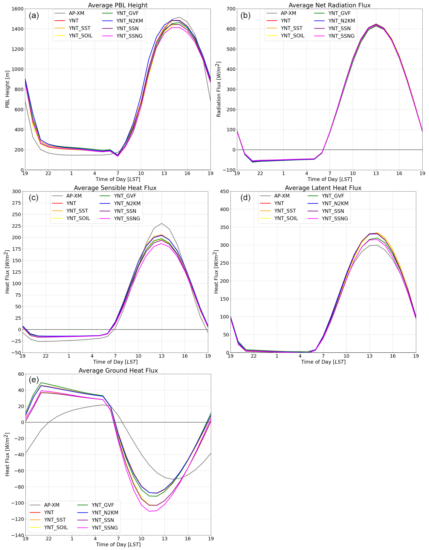
Figure 9 Same as Fig. 8, except for showing results on the 12 km domain. Time series were computed using simulated data from all stations located on the 1.3 km domain.

The lower accuracy of the AP-XM simulation could be due to limitations in the parameterization schemes when used at higher spatial resolution. This possibility is supported by Fig. 9, which shows the evolution of the PBL height and surface fluxes on the 12 km domain computed using simulated data from all stations on the 1.3 km domain. Differences between the AP-XM and YNT simulations are much smaller both in timing and magnitude on the 12 km domain. For example, the time series for PBL height, sensible heat flux, and latent heat flux are very similar for all of the simulations. Though the ground heat flux time series for the AP-XM simulation continues to be an outlier at this resolution, it now has the correct diurnal cycle with positive (negative) values during the night (day). The improved simulation of surface fluxes on the 12 km domain likely contributes to the more accurate temperature and wind speed analyses in the AP-XM simulation at that resolution (Fig. 3a–b and g–h). The presence of persistently higher latent heat flux (Fig. 9d) leads to a positive moisture bias in the AP-XM simulation (Fig. 3d–e); however, the bias is smaller on the 12 km domain than it was on the 1.3 km domain. Inspection of the surface energy fluxes and PBL height on the 4 km domain revealed larger differences between the AP-XM and YNT simulations (not shown) but not as large as those on the 1.3 km domain. Though it is not the focus of this research, differences in the PBL height between the AP-XM and YNT simulations could be due to differences in the vertical mixing strength and entrainment flux in the AMC2 and YSU PBL schemes (e.g., Hu et al., 2010). Together, these results show that the AP-XM simulation performs well at 12 km resolution but that its accuracy decreases with increasing model resolution.

4 Discussion and conclusions

In this study, eight WRF model simulations were performed to assess the impact of different parameterization schemes, surface datasets, and analysis nudging on the simulation of surface energy fluxes and near-surface atmospheric conditions in the Lake Michigan region during a 1-month period (22 May–22 June 2017) corresponding to the Lake Michigan Ozone Study field campaign. The simulations employed a triple-nested domain configuration containing 12, 4, and 1.3 km resolution grids, respectively. Two baseline simulations (AP-XM and YNT) employing different sets of parameterization schemes were performed to assess the importance of different physics suites. The YNT configuration additionally served as the baseline for six sensitivity simulations that were used to assess the impact of three satellite- and model-derived surface datasets and analysis nudging. Simulations were run, where standard climatological or coarse-resolution surface datasets were replaced by high-resolution, real-time datasets depicting lake surface temperatures, GVF, and soil moisture–soil temperature. Near-surface temperature, water vapor, and wind observations were used to assess the accuracy of each model simulation.

The AP-XM configuration generally produced more accurate near-surface analyses on the 12 km domain, with the exception of a moist bias in the 2 m water vapor mixing ratio, but its relative performance decreased with a finer model grid resolution. Evaluation of the AP-XM simulation showed that the diurnal evolution of the sensible and latent heat fluxes was similar to the YNT simulation on the 12 km domain but differed greatly on the 1.3 km nested domain, where it had much smaller sensible heat flux during the daytime and a larger latent heat flux at night. The increased latent heat flux combined with a shallower PBL contributed to the large moist bias in the 2 m water vapor mixing ratio. The evolution of the AP-XM ground heat flux was physically unrealistic on the 1.3 km domain because it remained negative at all times rather than changing signs between day and night (as seen during the YNT simulations). Because the evolution of the surface energy fluxes was more realistic on the 12 km domain, the poorer performance on the 4 and 1.3 km domains suggests that the Pleim–Xiu LSM is unable to adequately represent surface fluxes at higher resolutions. This could be due to its use of two soil layers, including a very shallow (1 cm) topsoil layer, that make it difficult to fully represent fine-scale features and soil heat fluxes. Increasing the number of soil layers in the Pleim–Xiu LSM could potentially improve its ability to simulate energy fluxes on high-resolution domains. In addition, use of observation nudging and soil moisture and soil temperature nudging as used in Torres-Vazquez et al. (2022) would also help constrain the evolution of this simulation. Though these specialized nudging techniques were not employed in our study due to their added complexity and confounding influence on the model evaluations because the same observations used in the nudging procedure would also be used to assess the accuracy of the simulations, their utility could be assessed in future work.

Inspection of the YNT statistics revealed a pattern in which the percentage change in the RMSEs for 2 m temperature, 2 m water vapor mixing ratio, and 10 m wind speed relative to the AP-XM baseline improved as the model resolution increased from 12 to 1.3 km. Switching to the YNT configuration led to substantial decreases in RMSE for 2 m temperature (25.8 %) and 2 m water vapor mixing ratio (14.9 %), and a more modest 3.3 % reduction in the RMSE for 10 m wind speed, when assessed using all stations on the 1.3 km domain. Despite the already large error reductions when using the YNT parameterization suite, additional improvements occurred in most variables when the high-resolution surface datasets were incorporated into the modeling platform. Evaluation of the YNT sensitivity experiments showed that the high-resolution soil dataset had the largest positive impact on temperature and water vapor errors and the second-largest impact on wind speed. Use of the GVF and SST datasets also led to more accurate temperature and water vapor simulations but some degradations in the wind speed, especially when using the GVF dataset. Only the simulation employing analysis nudging above 2 km produced more accurate 10 m wind speed analyses; however, 2 m temperature errors were larger along the western shoreline of Lake Michigan when the nudging was confined to levels above 2 km instead of above the PBL. This suggests that the modified nudging approach may not work well for areas near Lake Michigan where the PBL tends to be shallower because it reduces its ability to constrain the evolution of the lower troposphere. Despite this limitation, the most accurate near-surface simulations were obtained during the experiment that employed analysis nudging above 2 km, combined with the high-resolution SST and soil datasets. A slight degradation occurred when the satellite GVF dataset was included.

With these differences in near-surface temperature, humidity, and wind across model configurations and inputs, we can expect ensuing differences in the accuracy of model simulations of the production and transport of ozone precursors, in addition to the production of ozone. In Part 2 of this study (Pierce et al., 2023), we evaluate these impacts on ozone forecasts in the Lake Michigan region using meteorological analyses obtained from the baseline AP-XM and optimized WRF model configurations as input to CMAQ model simulations.