Ozone Monitoring Instrument (OMI) UV aerosol index data analysis over the Arctic region for future data assimilation and climate forcing applications

Due to a lack of high-latitude ground-based and satellite-based data from traditional passive- and active-based measurements, the impact of aerosol particles on the Arctic region is one of the least understood factors contributing to recent Arctic sea ice changes. In this study, we investigated the feasibility of using the ultraviolet (UV) aerosol index (AI) parameter from the Ozone Monitoring Instrument (OMI), a semi-quantitative aerosol parameter, for quantifying spatiotemporal changes in UV-absorbing aerosols over the Arctic region. We found that OMI AI data are affected by an additional row anomaly that is unflagged by the OMI quality control flag and are systematically biased as functions of observing conditions, such as azimuth angle, and certain surface types over the Arctic region, resulting in an anomalous “ring” of climatologically high AI centered at about 70^∘ N, surrounding an area of low AI over the pole. Two methods were developed in this study for quality-assuring the Arctic AI data. Using quality-controlled OMI AI data from 2005 through 2020, we found decreases in UV-absorbing aerosols in the spring months (April and May) over much of the Arctic region and increases in UV-absorbing aerosols in the summer months (June, July, and August) over northern Russia and northern Canada. Additionally, we found significant increases in the frequency and size of UV-absorbing aerosol events across the Arctic and high-Arctic (north of 80^∘ N) regions for the latter half of the study period (2014–2020), driven primarily by a significant increase in boreal biomass-burning plume coverage.

1 Introduction

The Arctic region experienced noticeable changes in climate over the past 2 decades (Serreze and Francis, 2006; Serreze and Barry, 2011; Dai et al., 2019). Notable are the rapid melting of Arctic sea ice (Comiso, 2012; Dai et al., 2019; Kwok and Rothrock, 2009), increased permafrost melting (Kokelj et al., 2017; Blunden and Arndt, 2019; Liljedahl et al., 2016), and shifts in wildfire activity (Xian et al., 2022b). Despite being identified as a major factor affecting the Arctic climate, atmospheric aerosol particles are still a large source of uncertainty in climate simulations (IPCC, 2013). Aerosol particles can alter the Arctic climate directly through reflecting/absorbing solar incoming energy and absorbing terrestrial emission of IR radiation (for micrometer-sized particles such as dust) and indirectly as cloud condensation nuclei by modifying cloud properties and increasing snow–ice melting through deposition of dust/smoke aerosols on snow- and ice-covered surfaces. All of these factors may very well interact between themselves and the overall Arctic meteorology resulting in a difficult sea ice prediction problem.

One of the limitations of current Arctic aerosol studies is that there are few spaceborne measurements from traditionally aerosol-sensitive instruments (both passive- and active-based). This is largely due to the bright and variable lower boundary conditions of snow, ice, and low clouds in the region (Martin, 2008). Consequently, there are no current operational aerosol retrievals that are available over the Arctic region from passive-based sensors such as the Moderate Resolution Imaging Spectroradiometer (MODIS), Multi-angle Imaging SpectroRadiometer (MISR), and Visible Infrared Imaging Radiometer Suite (VIIRS) (Xian et al., 2022a). Active sensors, such as the Cloud-Aerosol Lidar with Orthogonal Polarization (CALIOP) on board the Cloud-Aerosol Lidar and Infrared Pathfinder Satellite Observation (CALIPSO) satellite, are able to provide retrievals of aerosol vertical profiles regardless of the surface condition by measuring returned backscatter for the atmospheric layers below. Yet, CALIPSO's orbit only extends up to 82^∘ N, missing a large portion of the Arctic region, and CALIOP aerosol retrievals suffer from a “retrieval filled value” issue over or near the Arctic region due to the reduced sensitivity to optically thin aerosol layers (Toth et al., 2018).

The Ozone Monitoring Instrument (OMI), on board the Aura satellite, is a nadir-viewing spectrometer that measures backscattered solar radiation at channels both sensitive and not sensitive to ozone (Levelt et al., 2006). The OMI aerosol index (AI) is a semi-quantitative aerosol parameter that relates perturbations in UV radiance presumably caused by absorbing aerosols to an assumed radiance from a purely Rayleigh atmosphere and is able to detect UV-absorbing aerosols over bright surfaces such as clouds, deserts, snow, and ice (Torres et al., 2012; Alfaro-Contreras et al., 2014, 2016; Zhang et al., 2021). Launched in 2004, OMI provides one of the longest contiguous data records of the Arctic region at much higher spatial resolution than previous UV-sensitive spectrometers such as the Total Ozone Mapping Spectrometer (13×24 km² for OMI, 50×50 km² for TOMS). While widely used in scientific applications for detection of UV-absorbing aerosols over lower-latitude regions, OMI AI suffers from its own problems, including a well-known row anomaly issue that affects downstream products such as OMI AI (Torres et al., 2018) that could hinder aerosol analyses based on OMI AI in the Arctic. The OMI row anomaly first began in 2008 and is believed to be caused by a “physical obstruction”, with the number of affected rows growing and decreasing over the years and now affecting over 30 rows, or over 50 % of all OMI rows, and removing about one-quarter of coverage from each OMI swath. Further, long-period average AI fields demonstrate an unnatural pattern of seasonal “rings”. The ring, seen in the spring (April and May; Fig. 1a) and summer (June, July, and August; Fig. 1b), consists of high AI values in latitudes between approximately 70 and 80^∘ N and much lower AI values in latitudes north of approximately 80^∘ N. Additional high AI values are seen over shoreline regions in northern Russia, as well as along the ice–water boundary in the Greenland Sea.

In this study, we investigated uncertainties in OMI AI by enhancing this parameter's specificity by developing quality control methods. Using a revised and quality-controlled dataset, we studied extreme UV-absorbing aerosol events (dust and/or biomass-burning smoke; BB) over the Arctic region. Lastly, the developed OMI AI data may also be used for ongoing OMI AI data assimilation efforts over the Arctic region (e.g., Zhang et al., 2021).

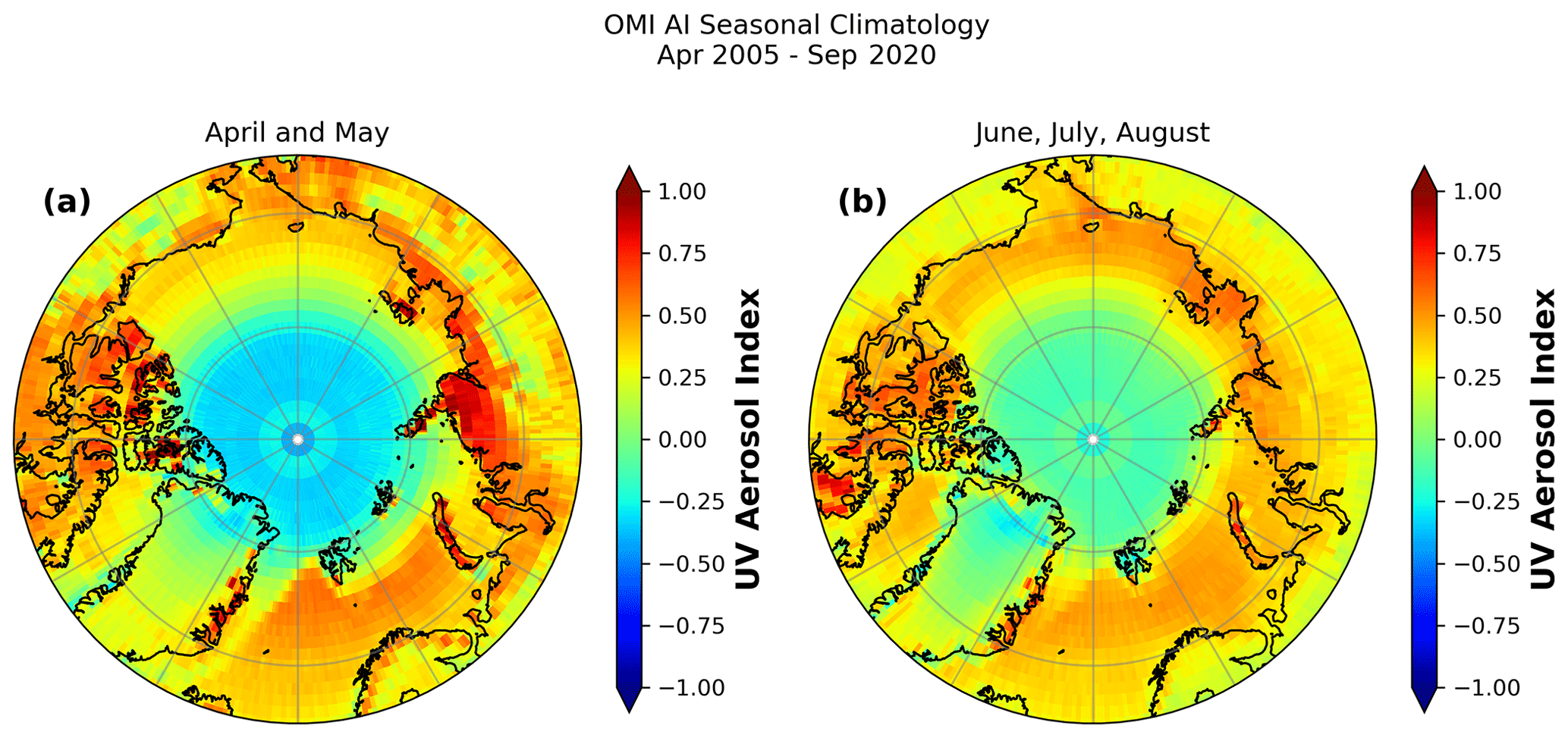
Figure 1 Spring (April, May) and summer (June, July, and August) climatological averages of pre-quality-control (QC) OMI aerosol index (AI) between April 2005 and September 2020.

2 OMI datasets

On board the Aura satellite with a ∼ 13:30 local equatorial crossing time, OMI measures reflected solar energy between 270–500 nm (Levelt et al., 2006). Using radiance measurements at the 354 nm spectral channel, the OMI aerosol index (ultraviolet aerosol index, UVAI) is derived based on Eq. (1):

$$\begin{array}{}\text{(1)}& \mathrm{UVAI}=-\mathrm{100}\log \left[{\displaystyle \frac{I_{\mathit{\lambda }}^{\mathrm{obs}}}{I_{\mathit{\lambda }}^{\mathrm{cal}}}}\right],\end{array}$$

where $I_{\mathit{\lambda }}^{\mathrm{obs}}$ is the observed radiance and $I_{\mathit{\lambda }}^{\mathrm{cal}}$ is the calculated radiance for a hypothetical pure Rayleigh scattering atmosphere. Over non-snow–ice surfaces, $I_{\mathit{\lambda }}^{\mathrm{cal}}$ for the operational product is calculated by considering both clear- and cloudy-sky contributions, but over snow–ice surfaces, $I_{\mathit{\lambda }}^{\mathrm{cal}}$ is calculated assuming a Lambertian surface reflectivity with no consideration of cloud cover status (Torres and Leonard, 2018). OMI OMAERUV V003 UV aerosol index data from the Aura OMI Level 2 near-UV aerosol data product “OMAERUV” are retrieved from the Goddard Earth Sciences Data and Information Services Center (GES DISC) archive for times between 1 April and 30 September each year from 2005 through 2020 (Torres, 2006). Sunlight is absent from the Arctic region during the boreal winter months, so only UVAI data between 1 April and 30 September of each year are analyzed.

3 Observed bias/uncertainties in OMI AI data

As the first phase of the study, to construct the quality-assured AI data for quantitative climatology and trend analysis of aerosol distributions over the Arctic region, we investigate uncertainties in the Arctic OMI AI data caused by the row anomaly and by observing condition dependencies.

3.1 Row anomaly

The first possible cause for the AI ring over the Arctic region as shown in Fig. 2 may be associated with the OMI row anomaly. In the OMI data, row anomalies are highlighted with a quality control flag named XTrackQualityFlag (Xtrack). The Xtrack values change from 0 to 4, representing a row as “not affected” (Xtrack value of 0); “affected, not corrected, do not use” (Xtrack value of 1); “slightly affected, not corrected, use with caution” (Xtrack value of 2); “affected, corrected, use with caution” (Xtrack value of 3); and “affected, corrected, use pixel” (Xtrack value of 4) by the row anomalies.

However, even after applying the Xtrack flag screening (by using OMI AI data with Xtrack = 0 only), additional bad sensor rows are found throughout the OMI data record (e.g., Fig. 2). As seen in Fig. 2a, which shows the OMI AI values for 10 April 2012 at 21:52:00 UTC, two rows (43 and 44) with significantly high AI values of above 3 are found in the middle of the swath, while the adjacent rows (45–50) report much lower AI. These same two rows report similarly high AI in the following swath on 10 April 2012 at 23:30:00 UTC (Fig. 2b), indicating that the AI signal in the two swaths is non-meteorological and is caused by the unflagged-row anomaly. The unflagged anomalous rows in the OMI dataset, which seem to exhibit a latitudinal dependence, must be identified and removed from further analysis.

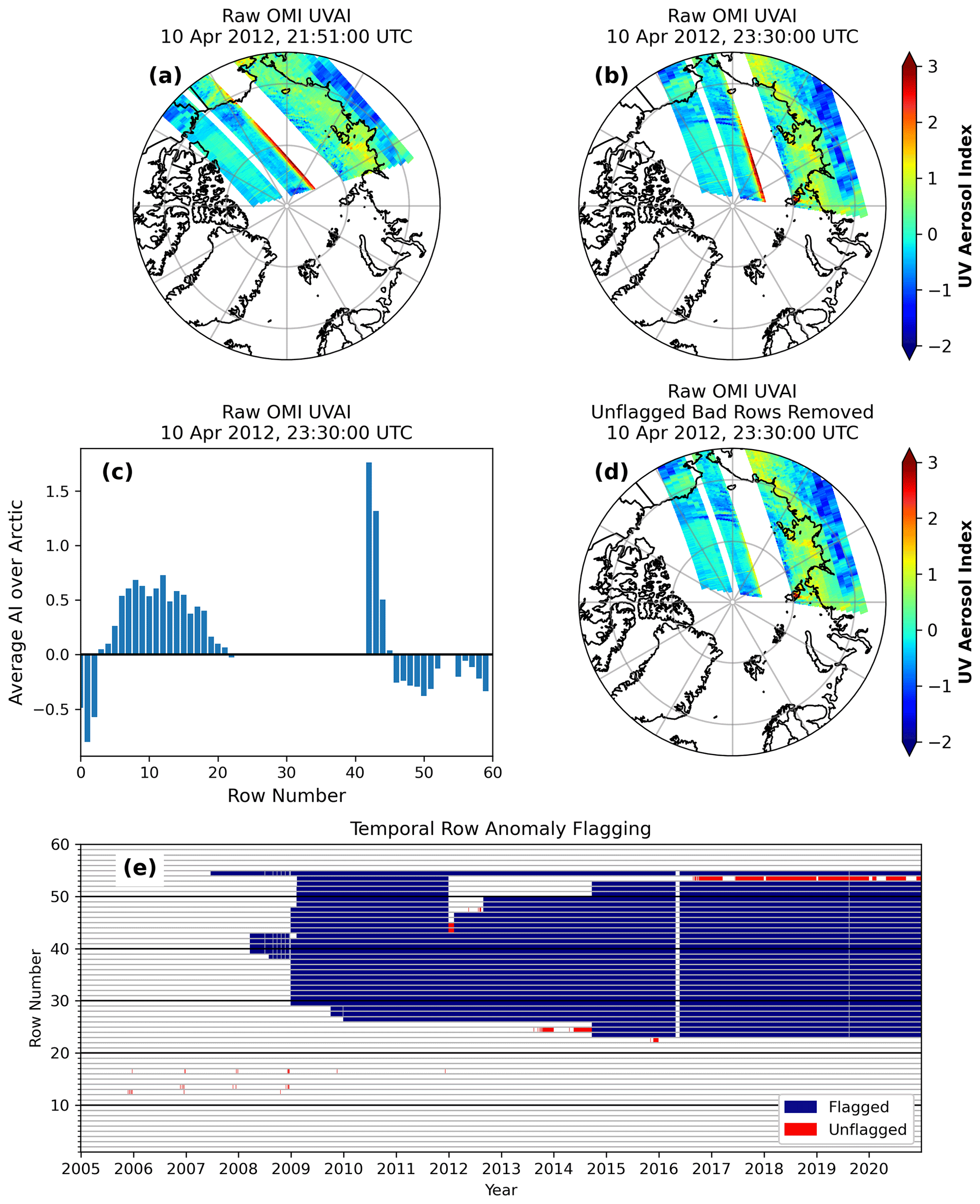
Figure 2 (a) Single-swath OMI UV aerosol index data from the swath from 10 April 2012 at 21:51:00 UTC. The large gap in the middle of the swath is caused by the removal of flagged-row anomaly-affected OMI data, while the red portion of the scan line over the Arctic is caused by the unflagged-row anomaly. (b) Single-swath OMI AI from 10 April 2012 at 23:30:00 UTC. (c) Averages of AI from each OMI sensor row over the Arctic from the swath from 10 April 2012 at 23:30 UTC. (d) Single-swath OMI AI from 10 April 2012 at 23:30:00 UTC but after removing anomalous rows 43 and 44 identified in panel (c). (e) Flagged- (blue) and unflagged-row (red) anomaly-affected OMI sensor rows not flagged by the XTrackQualityFlag variable in the OMI data files.

The first step in cleaning the OMI data is to remove the bad scan rows that are not flagged by the Xtrack flag through the entire study period of 1 April 2005 to 30 September 2020. Daily averages of AI from all 60 OMI sensor rows over the Arctic are calculated, and if any one of those 60 row averages is more than 2 standard deviations away from the mean of all 60 row averages, it is flagged as a bad row. For example, for the single OMI swath shown in Fig. 2b, the averages of the AI values from each row over the Arctic (Fig. 2c) reveal that the average AI in rows 43 and 44 is significantly higher than in the other rows, more than twice as large as any of the other row averages from the swath and nearly 400 % higher than nearby rows 47 and 48. Figure 2e shows the “flagged-” (blue) and “unflagged-row” (red) anomaly-affected rows in the Arctic OMI data between 1 April 2005 and 30 September 2020. The flagged rows in the figure reflect any row in which at least one pixel over the Arctic has a non-zero Xtrack quality control (QC) flag value, indicating that it is affected by the row anomaly. The unflagged rows are more than 2 standard deviations away from the average of all rows over the Arctic (indicating a row anomaly) but are not flagged by the Xtrack QC flag. As shown in Fig. 2e, the bad rows identified by the algorithm are variable across the dataset time period, with scattered unidentified bad rows found in the 10 s before 2012 and others in the 40 s found between 2012 and 2013. The most strongly affected unflagged rows found by the algorithm are rows 24, 22, and 53, with row 24 being contaminated from 2013 to 2015, row 22 being contaminated in 2016, and row 53 being contaminated from 2016 until at least the end of the time period. The unflagged bad rows found for each day are used in further analysis to pre-screen the AI data before applying the main QC methods.

3.2 Other observing-condition-related uncertainties

There are known limitations in the OMAERUV retrieval algorithm over topographically variable regions. The assumed surface pressure plays a critical role in the radiative transfer calculation of the Rayleigh atmosphere scattering necessary to determine the UV reflectance perturbation due to the absorbing aerosols. Thus, there are known AI biases in regions where the actual surface pressure varies from the pressure assumed by the OMAERUV algorithm, such as in mountainous regions (Colarco et al., 2017). In addition, over the Arctic, we found that AI patterns are highly dependent upon observing conditions such as surface properties and viewing geometry, likely associated with the retrieval algorithm. This can be illustrated by evaluating AI patterns over the same region for similar observing conditions but with observations separated by almost exactly 1 year. For example, the OMI swaths from 2 April 2007 at 00:51:00 UTC (Fig. 3a) and 1 year later on 2 April 2008 at 00:57:00 UTC (Fig. 3b) exhibit nearly identical AI patterns along the coast of northern Russia. Clearly, the repeated patterns in OMI AI indicate that they are systematic and are associated with surface properties and viewing geometries. Despite this observing condition dependency, aerosol events can still be detected using OMI AI data as shown in Fig. 3c and d. Figure 3c shows the OMI swath from 22 April 2007 at 15:19:00 UTC, and Fig. 3d shows the OMI swath from almost 1 year later on 22 April 2008 at 15:24:00 UTC (Fig. 3d). While similar patterns of moderate AI are observed along the northern Canadian and Alaskan coasts, the smoke plume extending over northern Alaska is still detectable in Fig. 3d. Figure 3 reveals that OMI AI data can still be used in an aerosol study over the Arctic region, but there are systematic biases in the OMI AI data that must be considered before using the data for quantitative scientific applications.

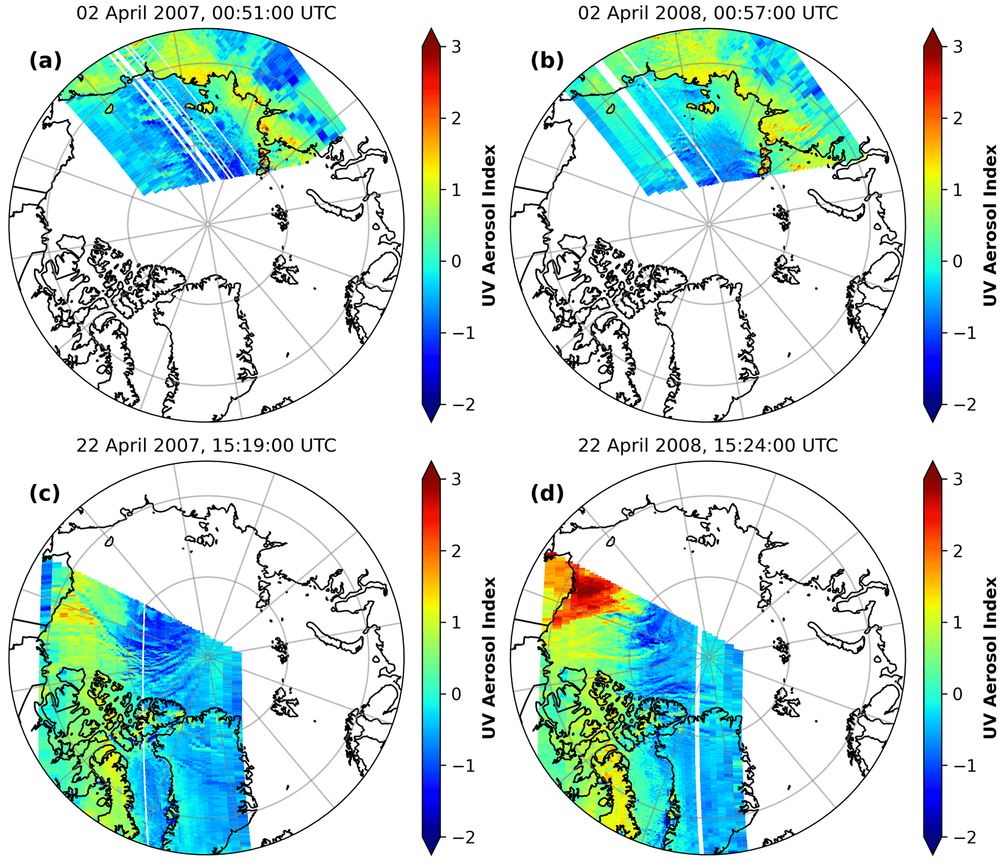
Figure 3 Single-swath OMI AI data from (a) 2 April 2007 at 00:51:00 UTC, (b) 2 April 2008 at 00:57:00 UTC, (c) 22 April 2007 at 15:19:00 UTC, and (d) 22 April 2008 at 15:19:00 UTC.

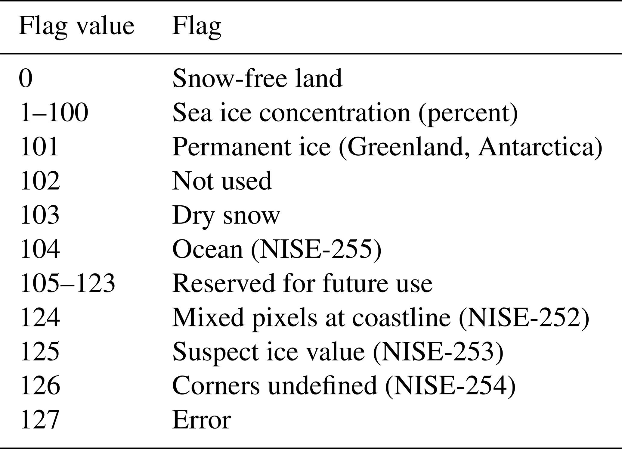
One of the causes for the systematic bias in OMI AI as seen in Fig. 3 is related to surface properties, with anomalously high AI values being associated with certain surface types. To examine the impact of surface properties on anomalies in OMI AI, we use the GroundPixelQualityFlags (GPQFs), which are included in the OMAERUV data. Each GPQF variable is a 16-bit unsigned integer, and different bit ranges are used to store different characterizations. Bits 0–3 contain the land–water flags, including “shallow ocean”, “land”, “shallow inland water”, and “deep inland water”. The bits of interest for studying the isolated high AI values are bits 8–14, which contain the snow–ice flags. The flag values (Table 1) contain flags for snow-free land, sea ice concentration from 1 % to 100 %, permanent ice (used mostly for Greenland and Antarctica), dry snow, and ocean, among others.

Table 1 OMAERUV snow–ice flags, taken from bits 8–14 of the GroundPixelQualityFlags found in each OMI data file. This table is adapted from information described in the OMI file specification document (Ahn et al., 2011). NISE: Near-real-time Ice and Snow Extent.

Anomalously high OMI AI values are found to be associated with the surface class “dry snow” for high latitudes, which denotes regions covered in seasonal snow, unlike the flag “permanent ice”, which denotes regions that are assumed to be covered with snow year-round (Stammes and Noordhoek, 2002). For example, the OMI AI data from the swath from 22 April 2008 at 10:27:00 UTC (Fig. 4a) show isolated regions around Greenland and the Canadian Arctic Archipelago with AI values of at least 2, much higher than the surrounding areas. The GPQF surface type classification values for the same swath (Fig. 4b) show that much of Greenland and the northeastern Canadian Arctic Archipelago are classified as permanent ice (seen as the cyan color in Fig. 4b), but there are also some areas classified as dry snow. The isolated areas of dry snow match up well with both the areas of isolated high AI in the single-swath AI data and the isolated climatologically high AI seen in the same regions in Fig. 1a. The isolated, anomalously high UVAI values in the Canadian Arctic Archipelago are found in the same places as the pixels classified as dry snow in the GroundPixelQualityFlags. This suggests that different algorithms are being used in the UVAI calculations between the two surface classification types. As mentioned in the data section (Sect. 2), different algorithms are applied over non-icy regions versus snow- and ice-covered regions (Torres and Leonard, 2018).

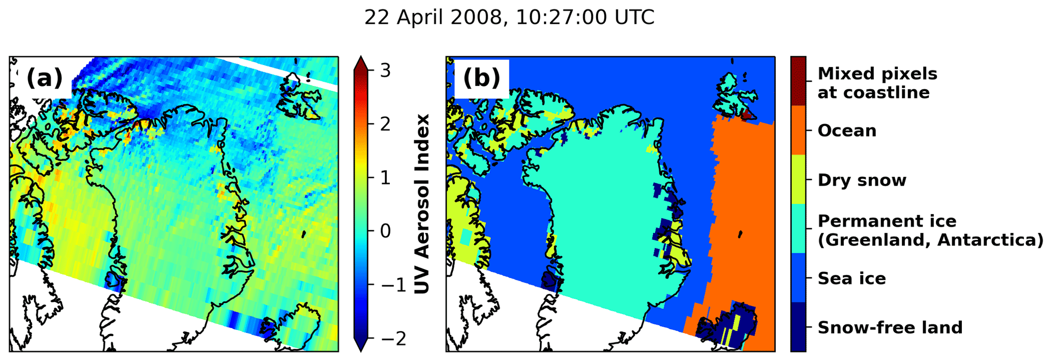
Figure 4 (a) Pre-QC OMI UVAI and (b) the surface type flag values extracted from the OMI GroundPixelQualityFlags from the OMI swath from 22 April 2008 at 10:27:00 UTC.

Another cause for the systematic bias in OMI AI is linked to azimuth angle or the row number. For example, Fig. 5a shows the average of all OMI AI data from each row over the Arctic between 1 April and 30 September 2006 (Fig. 5a, blue) and the relative azimuth angles for each OMI row (Fig. 5a, orange). OMI rows 1 to 30 have a relative azimuth angle of about 70^∘, and OMI rows 31 to 60 have a relative azimuth angle of about 110^∘. Not only is the average AI in rows 1 to 30 much higher than the average AI in rows 31 to 60, but also the average AI in rows 1 to 30 varies significantly as a function of row number. In contrast, the average AI in rows 31 to 60 does not vary as a function of row number and remains at about an average AI value of 0, with slight variation. This bias can be seen in OMI AI data from two aerosol-free swaths on 22 April 2006: one at 10:50:00 UTC (Fig. 5b) and another from two swaths later at 14:08:00 UTC (Fig. 5c). The OMI data from the 10:50:00 UTC swath over Greenland are sampled using the lower 30 scan lines and exhibit AI values near 1, which, by the definition of OMI AI, indicates the presence of UV-absorbing aerosols. Yet, large amounts of UV-absorbing aerosols are normally not expected over Greenland for this season (e.g., Xian et al., 2022b). The same region viewed with the higher 30 scan lines two swaths later exhibits much lower AI values below 0, indicating this region is free of UV-absorbing aerosols. Similar patterns can be routinely observed, with abnormal OMI AI values found for observations with row numbers of 1–30 (or a relative azimuth angle of below 100^∘). This suggests that systematic biases exist in OMI AI data associated with either row number or relative azimuth angle, and higher-than-normal OMI AI values are found for observations with a relative azimuth angle lower than 100^∘ or row numbers lower than 31.

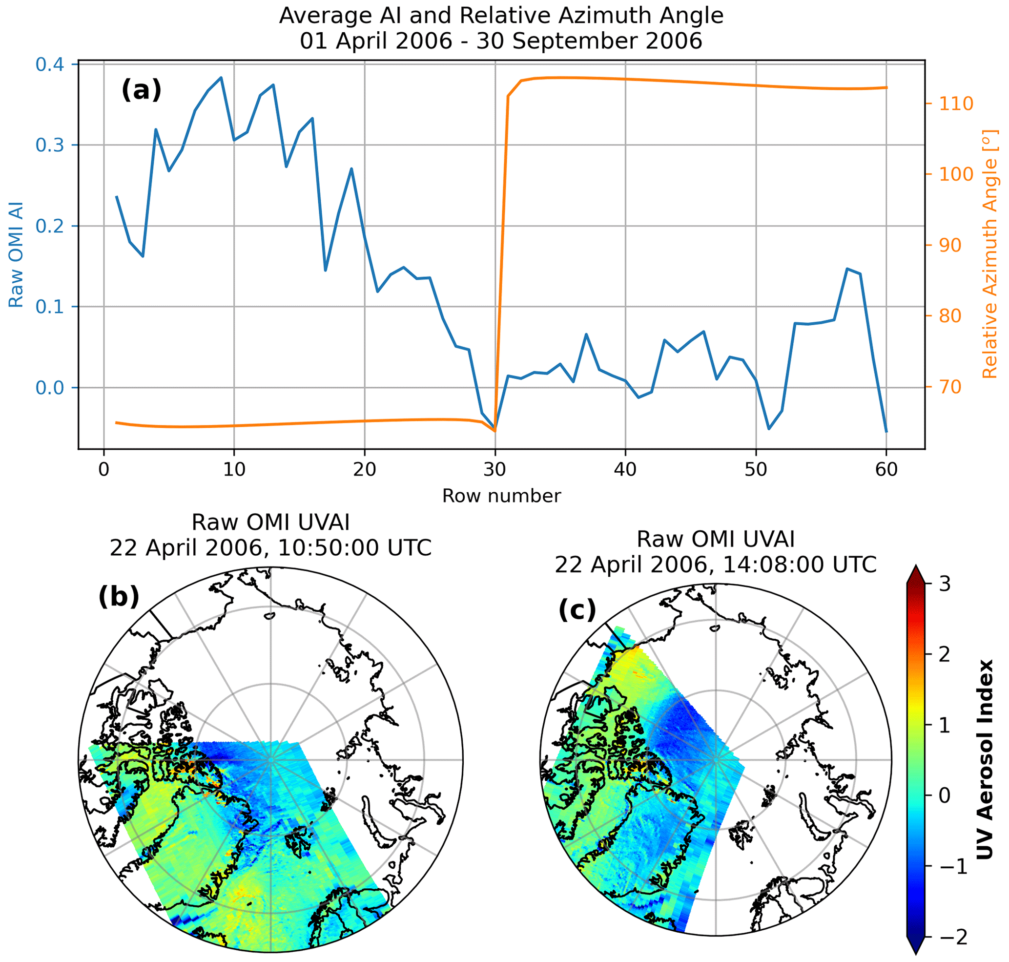
Figure 5 (a) Row-based climatology of OMI AI over the Arctic region calculated between 1 April and 30 September 2006 (blue) and the relative azimuth angle associated with each OMI sensor row from the OMI swath from 22 April 2006 at 10:50:00 UTC (orange). (b) OMI AI data from the OMI swath from 22 April 2006 at 10:50:00 UTC. (c) OMI AI data from the swath from 22 April 2006 at 14:08:00 UTC, two OMI swaths after the swath shown in panel (b).

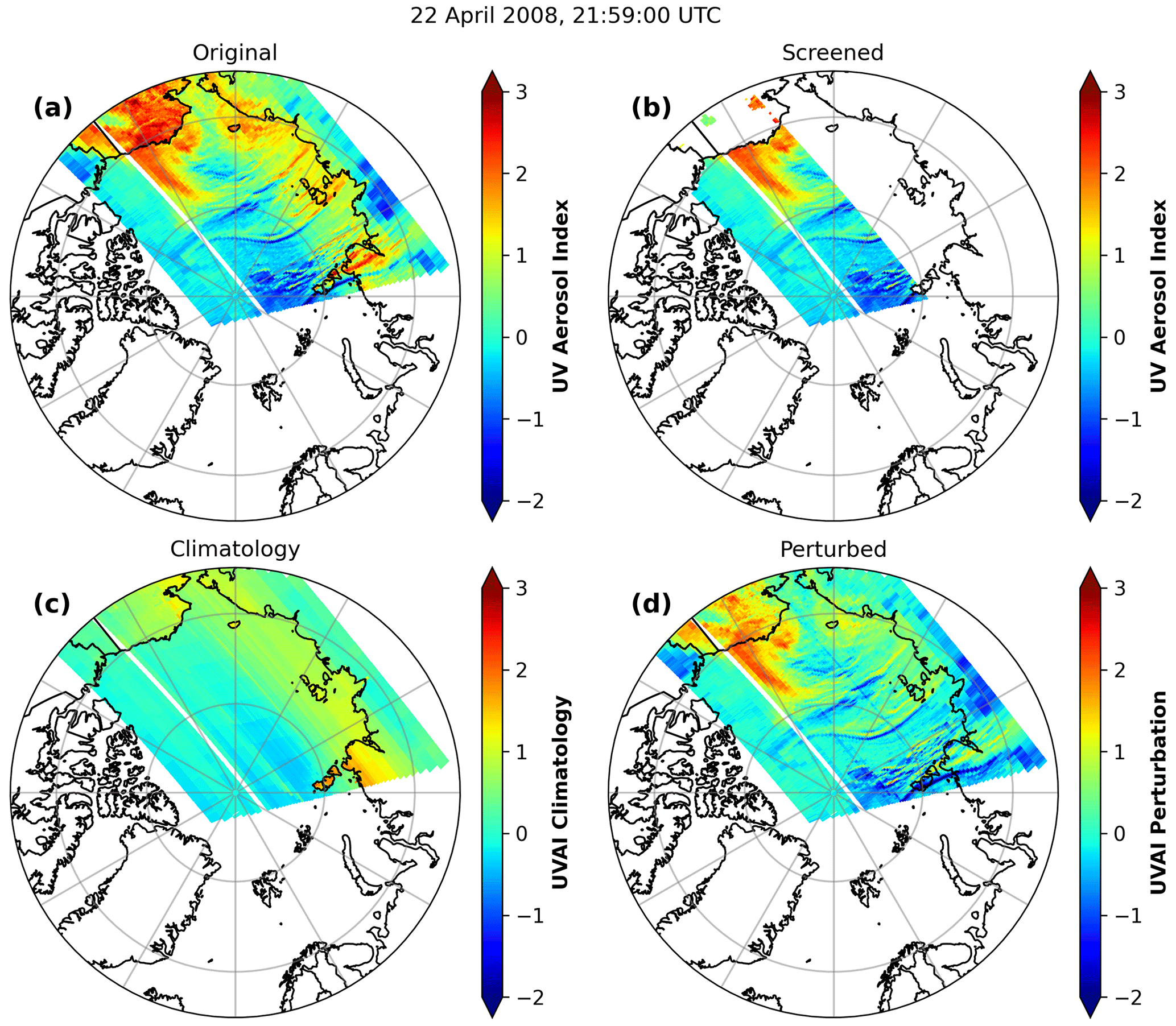
Figure 6 Results of applying the screening and perturbing QC methods to an OMI swath from 22 April 2008 at 21:59:00 UTC. (a) The raw, pre-QC OMI AI data. (b) The screened OMI AI data. (c) The binned climatological values associated with the SZA, VZA, AZM, ALB, and ground type values of each pixel from this swath. (d) The cleaned, perturbed AI data calculated after subtracting the climatology values from the pre-QC AI values.

4 Methods

4.1 Data QC methods

Knowing the issues in OMI AI data over the Arctic region, two different methods are presented for quality control of OMI AI data. In this first method, which is referred to as the “screening method”, all non-reliable data are removed. As discussed in the previous section, abnormally high OMI AI values are associated with certain surface types and low relative azimuth angles. Thus, AI pixels with a relative azimuth angle less than 100^∘, ground classification type of dry snow, and either flagged (Xtrack flag not equal to 0) or unflagged (as identified above) row anomaly are excluded. For the climatological study, we also used only rows 56–60, as we found that only rows 56–60 have a high relative azimuth angle larger than 100^∘ and are unaffected by a row anomaly through the entire study period (2005–2020). The advantage to the screening method is that unperturbed and quality-assured OMI AI data are included. Also, with the use of the same set of rows (56–60), the sampling bias is reduced (observations from the same set of rows are used in each month for the trend analysis as shown later, ensuring row-related bias is minimized). Still, due to the stringent selection criteria, only a small fraction of the data over the Arctic region pass this quality check. For example, for daily averages of AI for 17 July 2018 using only rows 56 through 60, only 12.2 % of all 0.25^∘ latitude–longitude boxes north of 65^∘ N contain data, compared to 51.1 % when all good rows are used. When all good rows are used, about 85 % of 0.25^∘ grid boxes between 70 and 80^∘ N have daily observation coverage, but that coverage drops to about 6 % when only rows 56 through 60 are used. North of 80^∘ N, only about 20 % of grid boxes have observation coverage in both methods because rows 56 through 60 are the only functional rows that sample in that region.

As discussed in the previous section and as shown in Fig. 4, OMI AI biases are strong and systematic functions of viewing geometries and surface conditions. Thus, in the second method, systematic patterns in OMI AI as functions of surface properties and viewing geometry are constructed using 15 years of OMI AI data over the Arctic region. Then, by excluding those systematic patterns, perturbations in OMI AI values can be derived and further used to study spatiotemporal trends of OMI AI over the region. This method is called the “perturbing method”. For this method, an OMI AI clear-sky climatology is constructed as a function of viewing geometry and ground classification for each month of the year (i.e., an April climatology contains data from April 2005, April 2006, etc.). As with the screening method, all bad rows from each day (both flagged and unflagged) are removed. Then, for a given monthly climatology, all OMI AI data from the associated month across all 15 years being analyzed in this study are binned by solar zenith angle (SZA), viewing zenith angle (VZA), relative azimuth angle (AZM), spectral albedo (ALB), and surface type (SFCT), with 2.5^∘ bins used for the SZA and VZA, 2.0^∘ bins used for the AZM, and the albedo bins being 0.05 wide. The addition of the SFCT dimension allows for the removal of AI data associated with faulty surface types, such as data over the regions of dry snow in the Arctic. Thus, for a given set of observing conditions, SZA, VZA, AZM, ALB, and SFCT values of each original OMI pixel are used to compute climatological AI values. Perturbations in OMI AI due to unrealized aerosol plumes are therefore identified. Note that the individual latitude and longitude of the OMI pixel are not used to bin the climatology. Also, the cloud fraction flag provided in the OMI L2 data was not used. Our tests showed that strict cloud screening methods (cloud fraction less than 0.2) removed much of the data over the snow- and ice-covered regions in the Arctic, indicating that there might be a potential misclassification issue in the OMI cloud flag over the Arctic region, which is not surprising as cloud detection over the Arctic from passive-based observations is a challenging topic.

Figure 6 shows an example of the results of applying both the screening and perturbing methods to the OMI swath from 22 April 2008 at 21:59:00 UTC. While a large smoke plume over Alaska and the Arctic Ocean is seen in the raw, pre-QC AI data (Fig. 6a), the pre-QC data also exhibit significant bias in AI across the sensor rows, with the lower scan lines near the Russian coast having generally higher AI than the higher scan lines over the Arctic Ocean. After applying the screening method to the AI data, the screened data (Fig. 6b) retain the AI signal north of Alaska while removing the biased rows with an azimuth angle less than 100^∘; however, the data volume is significantly reduced. Figure 6c shows the binned climatological values associated with the SZA, VZA, AZM, ALB, and SFCT values in each pixel from the swath. The climatological values reveal the row bias seen in the lower scan lines as well as the SFCT-induced bias over the coastal regions in northern Russia. Possible row anomaly effects are also seen in the mid-range scan lines, with several rows in the middle of the Arctic Ocean having slightly higher AI than the nearby rows. Figure 6d shows the perturbed AI data, calculated by subtracting the climatological AI values shown in Fig. 6c from the raw AI values shown in Fig. 6a. The AI signal over Alaska, as well as weak signal from the Russian coast, is retained, while the row- and SFCT-induced biases are removed. One downside of this approach is that the resulting cleaned dataset consists of AI perturbations. Thus, this approach is better suited to identifying the seasonal behavior and frequency of Arctic aerosol plumes.

4.2 OMI sensor drift check

It is necessary to explore potential signal drift and signal degradation in OMI AI data for trend analysis. To determine if any signal drift is present in the OMI AI dataset, monthly averages of AI are calculated for a remote-ocean region (0–40^∘ S, 180–140^∘ W) using the screening approach and with daily bad rows removed, as identified by the bad-row algorithm; total observation counts in the region for each month are tracked as well. The remote-ocean region is used as this region is assumed to be free from major aerosol pollution (e.g., Zhang and Reid, 2010). To reduce sampling bias, only data from rows 56 through 60 are included in this analysis. The observation counts (Fig. 7a, orange) decrease slightly from 2005 to 2012, with local minima in counts in 2009 and 2011, which reveals that at least one of the six rows used in the second analysis was contaminated for a short amount of time between 2009 and 2011; this confirms the row anomaly timeline reported by Torres et al. (2018). The average AI (Fig. 7a, blue) shows a similar dip between 2009 and 2011, but like the observation counts, it returns to the original average value of about 0.3 by 2012 and remains at about the same value until 2020, when a slight increase is found. We suspect that the increase in 2020 could be a result of the large Australian wildfires that occurred that year that spread smoke aerosols over the southern Pacific Ocean. No obvious signal drift is found in the data as shown in Fig. 7a between 2008 and 2019. To remove the effects of the seasonal cycle on the AI time series, we deseasonalize the monthly average AI data. While there is slight variation in the deseasonalized AI data from 2005 to 2020, shown in Fig. 7b most notably with the local minima in 2008 and the increase in 2020, these variations are generally small (less than 0.1 AI) and further show that there is no significant sensor drift in the OMI AI data.

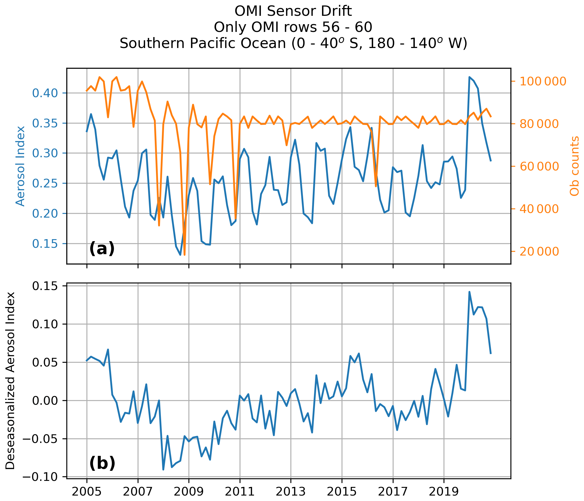
Figure 7 (a) Monthly average AI (blue) and total observation counts (orange) in a remote-ocean region in the southern Pacific Ocean (0–40^∘ S, 180–140^∘ W), calculated using the screening criteria and removing bad rows identified by the bad-row detection algorithm. (b) As in panel (a) but with deseasonalized monthly average AI.

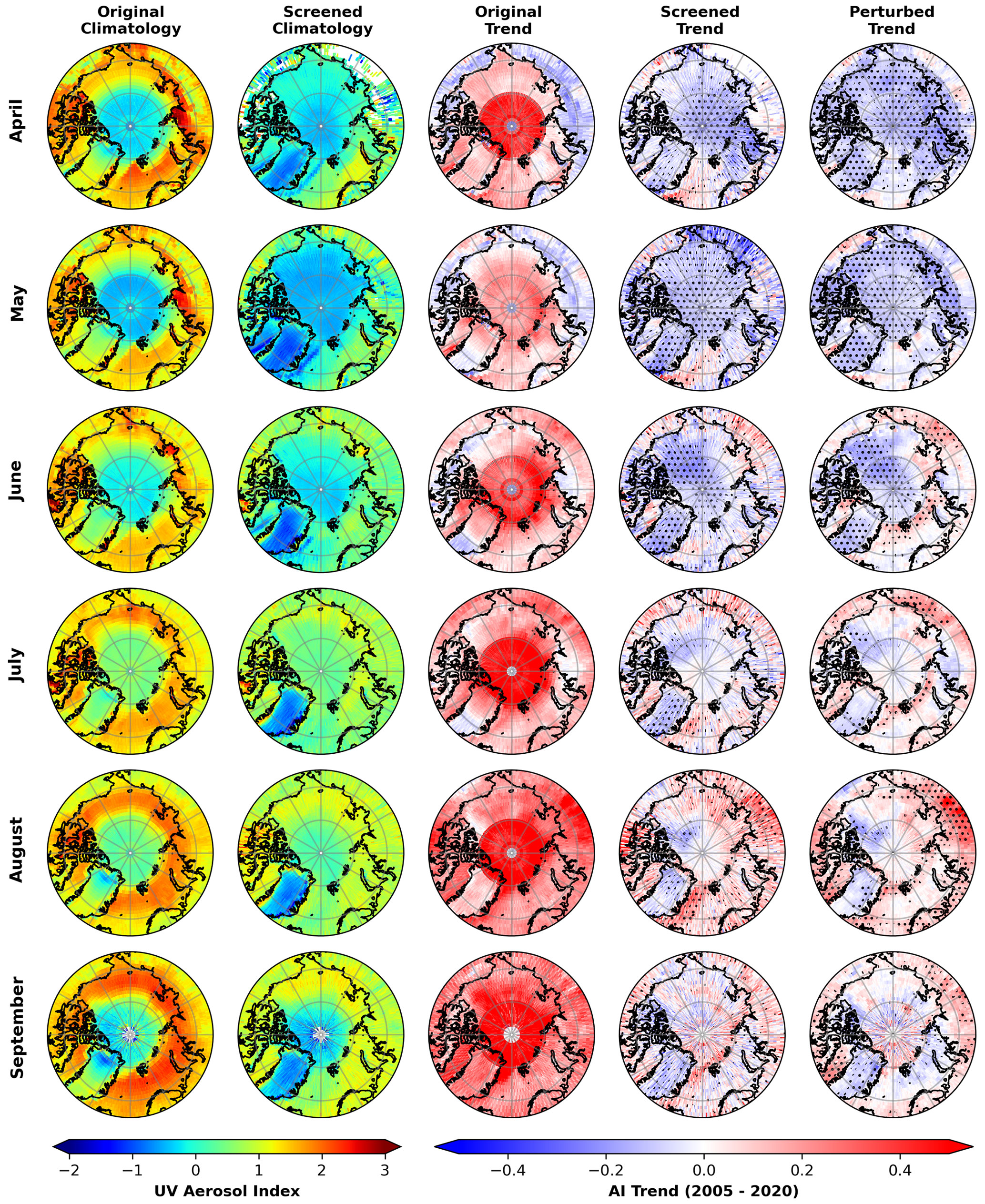
Figure 8 April (first and top row), May (second row), June (third row), July (fourth row), August (fifth row), and September (sixth and bottom row) monthly climatologies of pre-QC OMI AI data (first column) and screened AI data (second column), as well as trends in the non-quality-controlled AI data (third column), the screened AI data (fourth column), and the perturbed AI data (fifth column). Climatology and trend are calculated between 2005 and 2020. The dotted regions in the right two columns denote trends that are statistically significant at the 95 % confidence level.

4.3 OMI trend analysis

Trends are calculated for both the screened and the perturbed OMI AI data. Monthly averages of both the screened and perturbed OMI data are first calculated on a 1×1^∘ latitude–longitude grid. Then, monthly trends are calculated at each latitude–longitude grid point by performing linear regression on all averages from the month being analyzed; for example, if the May monthly trend is being calculated for a grid point, linear regression is applied to fit a line to the monthly averages from May of every year from 2005 through 2020. After the regression line is fitted to the data, the slope of the trend line is multiplied by the number of years in the study period to determine the AI trend over the study period. It is worth noting that the linear regression trend method may not be the most appropriate option in the case that the trends are driven by extrema, and the derived trend analyses may be sensitive to the choice of model for trend construction. To partially mitigate the issue, trend analyses are constructed on a monthly basis. Overall trend significance for each monthly trend at each grid box is calculated using a Wald t test (Wald, 1943), and trends are considered statistically significant if the p value from the Wald slope hypothesis test is less than 0.05, which denotes significance at the 95 % confidence level. The standard error of the trend (slope), which is a byproduct of the linear regression analysis, is also derived under the assumption of residual normality (Montgomery et al., 2021).

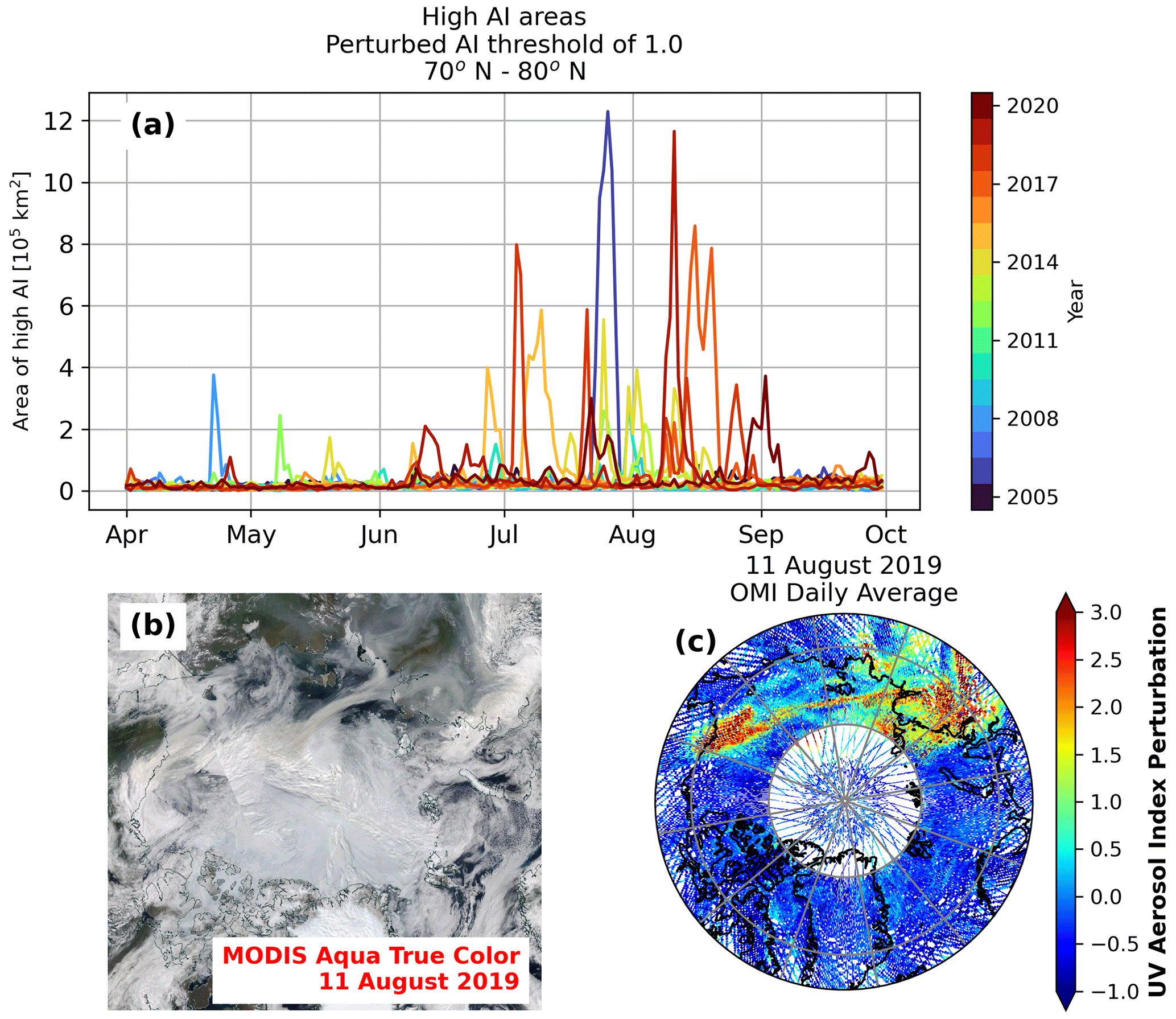
Figure 9 (a) Daily total area of 0.25^∘ latitude–longitude grid boxes between 70 and 80^∘ N with perturbed AI data greater than or equal to 1.0 between April 2005 and September 2020, with each time series colored by year. (b) MODIS Aqua true-color composite (obtained from the NASA Worldview site at https://worldview.earthdata.nasa.gov/, last access: 28 October 2022) imagery of an 11 August 2019 smoke plume extending from northern Russia into the Arctic Ocean. (c) The 0.25^∘ gridded perturbed OMI AI data for the 11 August 2019 BB aerosol event.

5 Arctic OMI AI climatology, trend, and extreme event statistics

5.1 Monthly climatology and trend of Arctic OMI AI

The screened and perturbed OMI data are applied to Arctic AI monthly summer climatology and trends for the time period from 2005 through 2020, as shown in Fig. 8. The first column in Fig. 8 shows the April, May, June, July, August, and September monthly AI climatology calculated without applying either of the QC methods, with only the original row anomaly check (Xtrack flag equal to 0) applied. A considerable ring effect is found in all six monthly climatologies, with the strongest ring effect found in August and September. The second column shows the same climatologies calculated using the screened OMI AI data. Not only is the overall climatological average significantly reduced, but also most of the AI ring found in the original climatologies is removed.

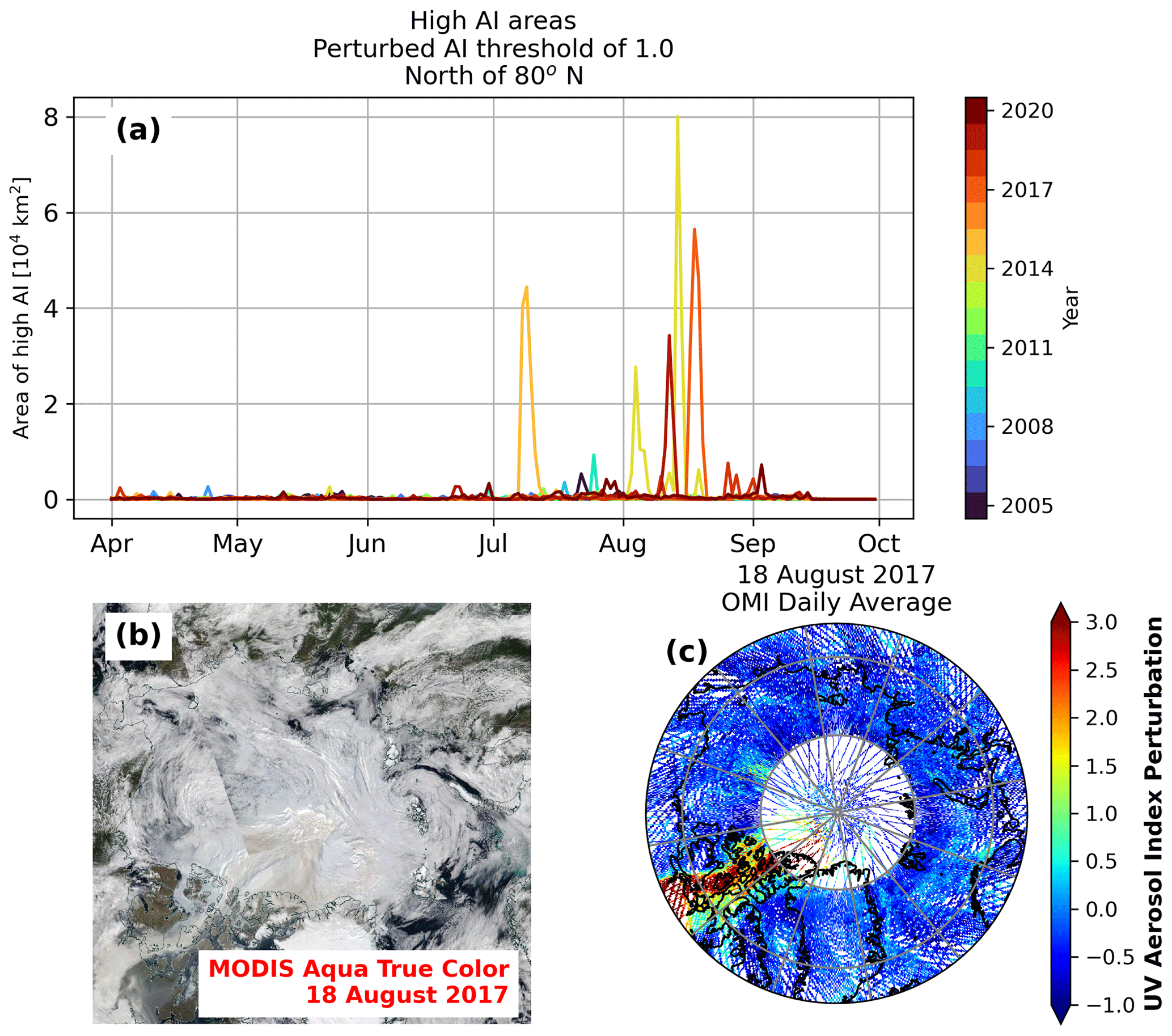
Figure 10 (a) As in Fig. 9 but for 0.25^∘ latitude–longitude grid boxes north of 80^∘ N. (b) MODIS Aqua true-color composite (obtained from the NASA Worldview site at https://worldview.earthdata.nasa.gov/) imagery of an 18 August 2017 smoke plume extending from northern Canada over the Arctic Ocean. (c) The 0.25^∘ gridded perturbed OMI AI data for the 18 August 2017 BB aerosol event.

The monthly trends calculated using the pre-QC OMI data, shown in the third column in Fig. 8, are very noisy, with an overall positive AI trend found across nearly the entire Arctic region in all analyzed months, as well as a ring of strong positive trend found north of approximately 80^∘ N. However, after applying both the screening (Fig. 8, fourth column) and perturbing (Fig. 8, fifth column) methods to the AI data, the overall positive AI trend is removed, with widespread statistically significant negative AI trends over the Arctic region found in the April and May monthly trends. The June and July monthly trends reveal increasing AI over northeastern Russia and Alaska, with the positive AI trends over Russia being statistically significant, while the August trends reveal increasing AI over north-central Russia and northern Canada, with the Russian positive AI trends being statistically significant. These results agree with aerosol optical depth (AOD) trend statistics simulated by chemical transport models assisted with MODIS, MISR, and CALIOP data analysis by Xian et al. (2022a), who found decreasing Arctic region AOD in the spring months and increasing Arctic region AOD in the summer months (Xian et al., 2022a). Maps of the standard error of the trend (found in the Supplement) corroborate the statistical significance shown in Fig. 8. The perturbed-trend standard errors are, overall, much lower than the screened-trend standard errors, and regions with statistically significant trends as shown in Fig. 8 are mostly associated with small trend standard errors.

Over the Arctic Ocean, mostly negative AI trends are found in June and July, with some areas of an increasing AI trend found over the Chukchi Sea (northwest of Alaska) in the July trends. A disagreement between the screened and perturbed trends exists in June and July, with the perturbed trends reporting a half circle of positive AI in the Kara and Greenland seas (north of Norway and northwest Russia) that is not found in the screened trends. This is likely due to the significant data coverage differences between the screened and perturbed datasets, with a single OMI swath in the perturbed dataset having much wider data coverage than the screened dataset. The consistently negative AI trends over the Greenland landmass for all months appear non-meteorological, as these negative trends are surrounded on all sides by positive AI trends over the ocean water. Due to the stark difference in trend between the oceanic and land-based trends over Greenland and the climatologically low AI over Greenland found in the screened AI climatology shown in Fig. 8, the negative AI trends over Greenland are suspected to be caused by issues of the lower boundary conditions and are not meteorological.

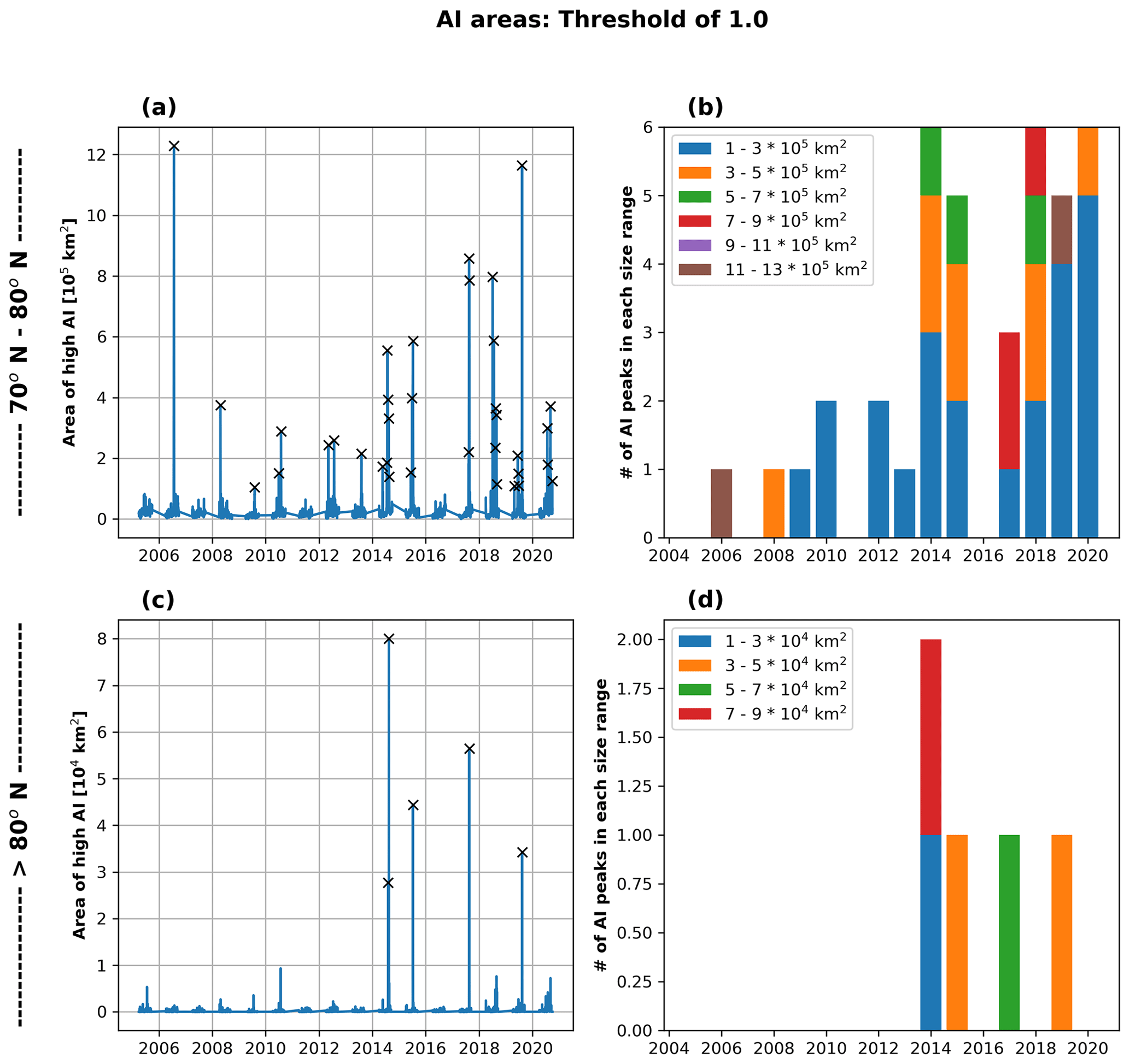
Figure 11 (a) Total time series of daily total areas of 0.25^∘ grid boxes with perturbed AI data greater than 1.0 for grid boxes between 70 and 80^∘ N. The black x symbols denote peaks in the perturbed AI data. (b) Yearly counts of peaks in each size range. (c) As in panel (a) but for grid boxes north of 80^∘ N. (d) As in panel (b) but for grid boxes north of 80^∘ N. Note that the y-axis values in panel (c) and the coverage bin areas in panel (d) are an order of magnitude smaller than in panels (a) and (b).

5.2 Arctic smoke plume frequency analysis

The perturbed AI dataset allows for a unique study of the frequency of aerosol events over the Arctic (70–80^∘ N) and high Arctic (north of 80^∘ N) that cannot be provided by other sensors. To study the Arctic aerosol event frequency, the perturbed AI dataset is averaged into daily 0.25^∘ latitude–longitude grids, and the total area of the 0.25^∘ grid boxes with average perturbed AI data beyond a threshold value is calculated for each day between 1 April 2005 and 30 September 2020. For this study, a threshold value of 1.0 for perturbed AI data is used to remove any residual non-meteorological noise from the data (note that results do not change significantly if the threshold is changed to a higher value such as 1.5 or 2.0). Figure 9a shows the time series of the daily total area of 0.25^∘ latitude–longitude grid boxes with perturbed AI data greater than 1.0 between 70 and 80^∘ N. Most Arctic aerosol events occur in July and August, with June having the next most aerosol events. Cool-colored lines in the figure indicate events occurring in the early portions of the study period (2005–2011), while warm-colored lines indicate events in the later portions of the study period. As shown, most of the large aerosol events between 2005 and 2020 occurred within the later portions of the study period. Additionally, this time series analysis of the gridded perturbed AI data allows for the identification of individual Arctic aerosol events, including a large BB aerosol plume that extended from Russia over the Arctic Ocean on 11 August 2019, shown in the Aqua MODIS true-color imagery found in Fig. 9b. The daily 0.25^∘ gridded perturbed AI data, shown in Fig. 9c, reveal a region of highly perturbed AI data across northern Russia, with a plume extending across the Arctic Ocean that closely matches the pattern found in the MODIS true-color imagery. The number of 0.25^∘ grid boxes north of Greenland that contain daily average AI values is much lower than in the regions over and south of Greenland because of the reduced coverage of OMI AI data from each swath caused by the row anomaly. Only the last five OMI rows in each swath provide coverage north of Greenland, while rows 1–22 provide additional coverage in the regions over and south of Greenland.

When restricting the analysis to latitudes only north of 80^∘ N, for latitudes and conditions that can largely only be sampled by OMI, a novel analysis into high-Arctic aerosol events may be completed. Figure 10a shows similar daily time series of total areas containing high values of perturbed AI as in Fig. 9 but using only 0.25^∘ grid boxes north of 80^∘ N. The number of large and small peaks is much smaller than in Fig. 9a, but as in Fig. 9a, the majority of the aerosol events occur in July and August. As indicated by the warm coloring of the small number of large peaks observed north of 80^∘ N in July and August, all high-Arctic aerosol events occurred in the latter portion of the study period. An example of one of these high-Arctic BB aerosol events is shown in Fig. 10b, which shows Aqua MODIS true-color imagery of a plume extending over the Arctic sea ice near the North Pole; the plume is seen as a darkened region over the sea ice north of Greenland. In the daily 0.25^∘ gridded perturbed AI data (Fig. 10c), the high-Arctic plume signal can be seen in the same region as the plume in the MODIS true-color imagery, but because the high-Arctic regions are only sampled by five OMI sensor rows, the spatial resolution is much lower.

To investigate patterns in the daily AI area time series shown in Figs. 9 and 10, the number of peaks in the daily AI area time series are calculated for each year, with the areas of each peak binned into size ranges. Figure 11a shows the total time series of high-AI (greater than 1.0) areas between 70 and 80^∘ N, with the x symbols indicating locations of peaks larger than 10⁵ km² in each year, while Fig. 11b shows the counts of high-AI peaks in each size range per year. As indicated by the number of x symbols in Fig. 11a and confirmed in the histogram shown in Fig. 11b, the number of high-AI peaks per year in the latter half of the study period (2014–2020) is much larger than the number of high-AI peaks per year in the earlier half of the study period (2005–2013). With the exception of 2016, every year between 2014 and 2020 saw at least three high-AI area peaks, while no year between 2005 and 2013 saw more than two high-AI area peaks. The size of the high-AI events also increased throughout the study period from 2005 through 2020. Aside from the very large high-AI event in 2006, all high-AI events in the first half of the study period were smaller than 5 × 10⁵ km², with only one reaching between 3 × 10⁵ and 5 × 10⁵ km² and reaching the second size bin. In the second half of the study period, many events occurred that were in the larger size bins. The high-AI area peaks north of 80^∘ N show similar results to the peaks north of 70^∘ N but with far fewer total events than in Fig. 11a and b. Figure 11c shows the daily total area of perturbed AI data higher than 1.0 north of 80^∘ N, with several large peaks found between 2014 and 2019. Unlike in Fig. 11a, in which there were several large BB aerosol events between 70 and 80^∘ N in the early half of the study period, there were no large-scale BB aerosol events in the first half of the study period north of 80^∘ N; this is further visualized in the histogram of peak size ranges shown in Fig. 11d. It is worth noting that it is difficult to draw clear conclusions on high-Arctic BB aerosol event trends from the results north of 80^∘ N due to the small sample size of only five large-scale BB events, but we still report that all large BB aerosol events in the high Arctic (north of 80^∘ N) between 2005 and 2020 occurred in the second half of the study period, between 2014 and 2020.

6 Conclusions

In this study, the feasibility of using OMI AI for studying spatiotemporal distributions of UV-absorbing aerosols was investigated. Issues in OMI AI data over the Arctic regions were studied, and two quality-controlled (QC) methods were developed for reducing bias and noise in OMI AI data for aerosol climate studies over the Arctic region. Lastly, quality-controlled OMI AI data from both methods were used for studying the spatiotemporal variations in UV-absorbing aerosols over the Arctic region for the study period of 2005–2020. We found the following.

1. Non-trivial uncertainties in OMI AI data over the Arctic region result in a ring of high AI at about 70^∘ N, surrounding a region of much lower AI over the North Pole. The uncertainties contributing to this anomalous ring signature include unflagged-row anomalies as well as systematic biases introduced by viewing geometry (e.g., higher bias is found for an azimuth angle less than 100^∘) and certain surface types such as the surface type dry snow.

2. Two methods were developed for quality control of OMI AI data over the Arctic regions. The screening method was developed for using only the “best” OMI AI data from rows 56–60. This method provides unperturbed AI estimates, yet the data volume is very limited. Some biases in OMI AI over the Arctic region are rather systematic and are functions of observing conditions. Thus, the perturbing method was developed for estimating perturbations in OMI AI values from their climatological means. The climatological means of 15 years of OMI AI over the Arctic region were constructed as functions of surface conditions and viewing geometry and were found to contain systematic biases of OMI AI for given observing conditions.

3. Using quality-controlled OMI AI data from the screening and the perturbing methods, spatiotemporal variations in OMI AI values were studied. We found decreasing AI values in spring and increasing AI over much of the Arctic region in the summer months, most notably in northern Russia and northern Canada in August, as well as decreasing AI over the Arctic Ocean north of Canada in June and July. Regional trends from both methods are largely consistent, although some differences can be found that may be due to the sampling differences between the two methods.

4. Using quality-controlled data from the perturbing method, we also studied extreme Arctic UV-absorbing aerosol events (defined by perturbed AI data greater than 1.0). We found increasing trends in the frequency and magnitude of high-AI aerosol events over both the Arctic (70–80^∘ N) and high-Arctic (> 80^∘ N) regions. In particular, north of 80^∘ N, no significant UV-absorbing aerosol events are found for the early part of the study period (2005–2013), yet a non-trivial number of significant UV-absorbing aerosol events are found in the latter part of the study period (2014–2020), mostly in summer months, indicating intrusions of aerosol plumes near or above the North Pole in recent years.

While the perturbed AI data generated for this study are designed for climatological and historical use, ongoing work is investigating the feasibility of directly assimilating the single-swath perturbed data into aerosol models for aerosol prediction over bright surfaces (Zhang et al., 2021). It is also worth noting that while not used in this study due to its relatively short data record, the TROPOspheric Monitoring Instrument (TROPOMI) also provides observations at the UV and near-UV spectrum with a much finer spatial resolution than OMI (3.5×7 km² nadir pixel size compared to OMI's 13×24 km² nadir pixel size) yet without the row anomaly suffered by OMI (Veefkind et al., 2012). UVAI from TROPOMI can and should be used for Arctic aerosol studies in the future.