Measurement report: Atmospheric CH₄ at regional stations of the Korea Meteorological Administration–Global Atmosphere Watch Programme: measurement, characteristics, and long-term changes of its drivers

To quantify CH₄ emissions at policy-relevant spatial scales, the Korea Meteorological Administration (KMA) started monitoring its atmospheric levels in 1999 at Anmyeondo (AMY) and expanded monitoring to Jeju Gosan Suwolbong (JGS) and Ulleungdo (ULD) in 2012. The monitoring system consists of a cavity ring-down spectrometer (CRDS) and a new cryogenic drying method, with a measurement uncertainty (68 % c.i. (confidence interval)) of ± 0.7–0.8 ppb. To determine the regional characteristics of CH₄ at each KMA station, we assessed the CH₄ level relative to local background (CH_4xs), analyzed local surface winds and CH₄ with bivariate polar plots, and investigated CH₄ diurnal cycles. We also compared the CH₄ levels measured at KMA stations with those measured at the Mt. Waliguan (WLG) station in China and Ryori (RYO) station in Japan. CH_4xs followed the order AMY (55.3 ± 37.7 ppb) > JGS (24.1 ± 10.2 ppb) > ULD (7.4 ± 3.9 ppb). Although CH₄ was observed in well-mixed air at AMY, it was higher than at other KMA stations, indicating that it was affected not only by local sources but also by distant air masses. Annual mean CH₄ was highest at AMY among all East Asian stations, while its seasonal amplitude was smaller than at JGS, which was strongly affected in the summer by local biogenic activities. From the long-term records at AMY, we confirmed that growth rate increased by 3.3 ppb yr⁻¹ during 2006/2010 and by 8.3 ppb yr⁻¹ from 2016 to 2020, which is similar to the global trend. Studies indicated that the recent global accelerated CH₄-growth rate was related to biogenic sources. However, δ¹³CH₄ indicates that the CH₄ trend in East Asia is derived from both biogenic and fossil fuel sources from 2006 to 2020. We confirmed that long-term high-quality data can help understand changes in CH₄ emissions in East Asia.

1 Introduction

Atmospheric methane (CH₄) is an important greenhouse gas and is one of the main drivers of climate change. The global atmospheric CH₄ abundance was 1889 ± 2 ppb in 2020, increasing 2.6 times since 1750 (∼ 722 ppb, pre-industrial period); the relative CH₄ increase since the pre-industrial period is greater than other major greenhouse gases such as CO₂ (1.5 times) and nitrous oxide (1.2 times) (Crotwell et al., 2022). Recently, CH₄ has gained substantial interest because of its relatively shorter lifetime in the atmosphere (∼ 9 year) compared with that of other long-lived greenhouse gases (Prinn et al., 2005). CH₄ emission reduction may thus be an effective method to partially mitigate climate change. The Sixth Assessment Report by the Intergovernmental Panel on Climate Change (IPCC) reported that, if strong and sustained CH₄ emission reductions are integrated with air pollution controls, net warming could decrease in the long term because of the short lifetime of both CH₄ and aerosols (Masson-Delmotte et al., 2021).

To reduce the atmospheric CH₄ burden, its emissions and sinks must first be quantified. CH₄ loss is primarily attributed to reaction with hydroxyl radicals (OH), which are part of atmospheric photochemical cycles, while there are various natural (wetlands, freshwaters, and geological) and anthropogenic CH₄ sources (agriculture, waste, fossil fuels, and biomass burning) with different spatial and temporal distributions (Lan et al., 2021; Basu et al., 2022). Because of their diverse sources in different regions, high-resolution, quality data can help quantify the atmospheric CH₄ budget.

In the World Meteorological Organization Global Atmosphere Watch Programme (WMO/GAW), there are 170 stations that monitor atmospheric CH₄ but with poor spatial coverage in Asia (https://gawsis.meteoswiss.ch, last access: November 2021).

Among CH₄ sources, rice agriculture is intense in Asia, mainly in China and India (Kai et al., 2011). China also has the largest anthropogenic CH₄ emissions in the world, mainly from solid fuel (34 %), rice cultivations (20 %), and enteric fermentation (10 %) (Janssens-Maenhout et al., 2019; Crippa et al., 2022). South Korea ranks among the world's top three importers of liquefied natural gas (LNG), following Japan and China (https://eia.gov/international/analysis/country/KOR, last access: November 2021). South Korean major CH₄ emissions are derived from wastewater treatment (40 %), enteric fermentation (22 %), and then rice cultivations (14 %) (Crippa et al., 2022). In this regard, the Korea Meteorological Administration (KMA) WMO/GAW network is important to understand not only the South Korean CH₄ flux but also that of the Asian continent, as it is sensitive to air masses transported from Asia and especially from China.

South Korea's atmospheric CH₄ monitoring history started at Tae-Ahn Peninsula (TAP; 36.74^∘ N, 126.13^∘ E; 20 m above sea level) by the Korea Centre for Atmospheric Environment Research in the western part of South Korea in 1990, with weekly flask-air sample collection as a part of the U.S. National Oceanic and Atmospheric Administration (NOAA), Global Monitoring Laboratory (GML), Cooperative Global Air Sampling Network (https://gml.noaa.gov/ccgg/about.html, last access: 29 May 2023). Since 1999, the KMA has been monitoring atmospheric CH₄ with quasi-continuous measurements at Anmyeondo (AMY; 36.53^∘ N, 126.32^∘ E; a 40 m tower whose base is 46 $\mathrm{m}\mathrm{a}.\mathrm{s}.\mathrm{l}.$), approximately 28 km from TAP. In 2012, the KMA expanded its monitoring network to capture data from the southwest (Jeju Gosan Suwolbong, JGS; 33.30^∘ N, 126.16^∘ E) and east (Ulleungdo, ULD; 37.48^∘ N, 130.90^∘ E) of South Korea to cover the entire peninsula for a better understanding of CH₄ sources and their characteristics. However, there is no published description of measurement quality, regional characteristics, and long-term trends of CH₄ for the KMA WMO/GAW network.

A few studies reported that CH₄ levels are affected by emissions from Russian wetlands and local rice cultivation near TAP (Dlugokencky et al., 1993; Kim et al., 2015). In 2019, observations at AMY indicate larger emissions compared with previous years, which were caused by soil temperature and moisture changes (Kenea et al., 2021). In summer, high atmospheric CH₄ levels were observed in airborne measurements because of biogenic sources such as rice paddies, landfills, and livestock (Li et al., 2020). The observed atmospheric ratio, ${\mathrm{CH}}_{\mathrm{4}}/{\mathrm{C}}_{\mathrm{2}}{\mathrm{H}}_{\mathrm{6}}$, was 53 ppb ppb⁻¹ during the KORUS-AQ campaign from May to June 2016, which is related to fossil fuel use in Seoul and Busan, while it was 150 to 250 ppb ppb⁻¹ in southwestern South Korea, related to biogenic emissions such as rice paddies (Li et al., 2022). These studies indicate CH₄ emissions sources are diverse in South Korea based on a short-term campaign study. Therefore, it can be difficult to figure out the representative long-term and regional characteristics in Korea. Also, even if CH₄ is monitored long-term at regional scale, poor measurement quality can lead to misinterpretation of the CH₄ budget, preventing development of science-based policies. Additionally, both measurement uncertainty and inadequate assessment of background air can limit the accuracy of observation-based estimates for local- or regional-scale greenhouse gas emissions (Graven et al., 2012; Turnbull et al., 2009, 2015; Lee et al., 2019).

In this paper, we present CH₄ data quality procedures and processing methods at three KMA monitoring stations, including measurement uncertainties. We analyzed the characteristics of CH₄ at the KMA stations from 2016 to 2020 and compared the data with those collected at other stations in East Asia: the global background WMO/GAW station in Waliguan (WLG; 36.28^∘ N, 100.90^∘ E; 3810 m), China, and the WMO/GAW station in Ryori (RYO; 39.03^∘ N, 141.82^∘ E; 260 m) in Japan, which reflects the global growth rate (Watanabe et al., 2000). In addition, we investigated the changes in CH₄ enhancement from 2006 to 2020 and analyzed source regions based on measurements of ${\mathit{\delta }}^{\mathrm{13}}{\mathrm{C}}_{\left({\mathrm{CH}}_{\mathrm{4}}\right)}$ in flask-air samples to trace the major source changes. Furthermore, this study can serve as a reference for KMA data archived at the World Data Centre for Greenhouse Gases.

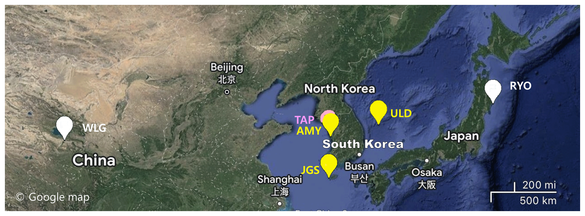
Figure 1 Locations of KMA CH₄ monitoring stations in South Korea: Anmyeondo (AMY; 36.53^∘ N, 126.32^∘ E), Jeju Gosan Suwolbong (JGS; 33.30^∘ N, 126.16^∘ E) and Ulleungdo (ULD; 37.48^∘ N, 130.90^∘ E). Tae-an Peninsula (TAP; 36.74^∘ N, 126.13^∘ E), part of NOAA's flask-air sampling network, is 28 km from AMY in South Korea. Mt. Waliguan (WLG; 36.28^∘ N, 100.90^∘ E) and Ryori (RYO; 39.03^∘ N, 141.82^∘ E) are located in China and Japan, respectively. This map is derived from Google Maps.

Table 1 Information on the three KMA CH₄ monitoring stations in South Korea.

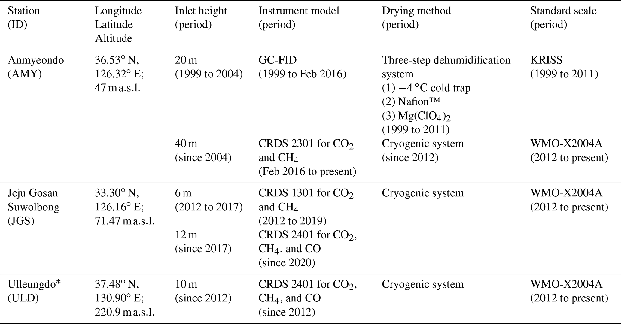
^∗ ULD is not registered in the GAW network.

2 Experiment

2.1 Sampling sites

The locations of AMY, JGS, and ULD stations are shown in Fig. 1, and summaries of the measurement systems are in Table 1. Detailed information was provided in Lee et al. (2019). Only key information focusing on CH₄ is summarized here.

AMY is located in the western part of South Korea, approximately 28 km south of TAP and 130 km southwest of the megacity of Seoul. Within 50 km of AMY, the second largest rice paddies and largest livestock industry of South Korea are present. The largest coal and heavy oil-fired thermal power plants in South Korea are within 35 km of this station, to the northeast and southeast, respectively, and the largest LNG power plant in South Korea is 100 km to the north east of this station. The local region mainly consists of agricultural land growing rice, sweet potatoes, and onions, and the area is also known for its leisure opportunities during summer. The west and south sides of AMY are open to the sea, with a large tidal mudflat with many pine trees along the coast.

JGS is located in the western part of Jeju Island, which is the largest volcanic island (1845.88 km²) in the southwest of Korea and is approximately 90 km from the mainland. The major industries here are tourism and livestock, focusing on horses and pigs. JGS is located within a famous UNESCO Global Geopark that has outcrops of volcanic deposits exposed along the coastal cliff. Next to JGS, agriculture is widespread, with potatoes, garlic, and onions being the main crops in the largest plain in Jeju Island. The station is open to the sea from the southwest to northwest, with the cliffs comprising volcanic basalt rocks. The sea to the south is connected to the East China Sea, and the sea to the west is linked to the Yellow Sea.

ULD is located in the east of Ulleungdo Island, which is in the eastern part of Korea and approximately 155 km from the mainland. In the southeastern part of the Korea Peninsula, numerous steel, chemical, and petrochemical industries are present along the coastline, within approximately 200–250 km from the island. There are two large natural gas power plants. Ulleungdo Island covers 72 km² and has a volcanic origin, being a rocky steep-sided island that is the top of a large stratovolcano that has a maximum elevation of 984 m. This peak is located northwest of ULD. There are a few small mountains with heights from 500 to 960 $\mathrm{m}\mathrm{a}.\mathrm{s}.\mathrm{l}.$, within 5 km to the north and southeast of the station. Because of those geological features, ULD is mainly affected by airflow from over the hill to the southwest and by downslope winds from northeast. In the southwestern area, there is a small brickyard 200 m from the station and a garbage incinerator within 100 m. The garbage incineration facility was moved to the north side of island in December 2016. Therefore, many studies do not include the data before 2017. Farming and fishing industries are very active on the island, although there are no farms in the southern area. An automatic weather station (AWS) was installed at AMY near the air sampling inlet and 10 m above the station at JGS and ULD, independent from the air inlet tower.

2.2 Measurement environment and instrument

At all three stations, the measurement system consists of (1) an inlet, (2) a pump, (3) a drying system, and (4) an analyzer. Detailed information of the system was discussed by Lee et al. (2019).

1. Inlet. Dekabon sampling tubing (Nitta Moore 1300-10, i.d. 6.8 mm, o.d. 10 mm, high-density polyethylene jacket, overlapped aluminum tape, and ethylene copolymer liner) with a stainless-steel filter (D 4.7 cm, pore size 5 µm) was mounted on a plastic mesh holder installed on the intake and connected to the pump. The inlet height was changed at AMY in 2004 and at JGS in 2017 (Table 1).

2. Pump. A KNF diaphragm pump (N145.1.2AN.18, Germany, 55 L min⁻¹, 7 bar in AMY; N035AN.18, Germany, 30 L min⁻¹, 4 bar in JGS and ULD) is installed between the inlet and drying system.

3. Drying system. Sample air is dried with a cryogenic method (CT-90, Operon, Korea). Inside the drying system, there are two chambers with two steps; ambient air is cooled to −20 ^∘C in the first chamber and then to −50 ^∘C in the second chamber. This system was installed in 2012 at all three KMA stations. This system dried the sampled air enough so that the bias from the humidity is negligible. This is described in Sects. 2.3 and 3.1.

4. Analyzer. A model G2301 (Picarro, USA) was installed in October 2011, and it became the official CH₄ measurement system at AMY, starting on 1 February 2016. Before February 2016 (G2301), a GC-FID (gas chromatograph with a flame ionization detector) was used to monitor atmospheric CH₄. The cavity ring-down spectrometer (CRDS) recorded atmospheric CH₄ every 5 s across the KMA WMO/GAW network, while the GC-FID measured CH₄ every 30 min. At JGS, the monitoring of atmospheric CH₄ started with the use of G1301 in 2012, which was changed to G2401 from 2020. G2401 has been used from 2012 at ULD.

2.3 Calibration method

Our highest-level standards are designated “laboratory standards”. We have four laboratory standards prepared by the WMO/GAW Central Calibration Laboratory (CCL) on the WMO-X2004A scale in the range 1700 to 2500 ppb with uncertainties of less than 2 ppb (95 % confidence level, coverage factor k=2, https://gml.noaa.gov/ccl/ch4_scale.html, last access: 5 January 2023). They are provided in 29.5 L aluminum cylinders (Luxfer, UK) by the CCL filled with 130 bar (https://gml.noaa.gov/ccl/services.html, last access: 5 January 2023). Our laboratory standards have been recalibrated every 3 years or replaced with new sets since first use in 2012, according to GAW recommendations. Remaining pressure in each cylinder is still high, ∼ 100 bar.

For working standards, dry, ambient air is compressed into a cylinder at AMY with a range of roughly 1800–2500 ppb. To bracket the measurement range, we diluted collected air to around 1700 ppb with zero air.

Filled working standards are sent to a central laboratory of the National Institute of Meteorological Sciences (NIMS) in Jeju for calibration against the laboratory standards. The scale was transferred with a CRDS (G2401, Picarro, USA). The scale propagation uncertainty is described in Sect. 3.1.

Normally the difference in H₂O between laboratory and working standards measured by CRDS is ∼ 0.00054 %, which leads to a bias of 0.01 to 0.014 ppb for CH₄ in the given range according to the Eq. (1) from Rella et al. (2013). This value is negligible, so it was not considered as a factor for the propagated uncertainty

$$\begin{array}{}\text{(1)}& {\displaystyle \frac{C_{\text{dilution}}}{C_{\text{dry}}}}=\mathrm{1}-\mathrm{0.01}{H}_{\text{act}},\end{array}$$

where C is the CH₄ mole fraction, and H_act is the water mole fraction difference between laboratory and standard gases (in %). For example, 0.00054 % H₂O difference between two cylinders causes 0.01 ppb bias at 1800 ppb.

Analyzer response had been calibrated every 2 weeks for all stations before December 2019, but it was changed to 5 or 6 d with different calibration frequency at each station based on the reproducibility; all four working standard gases with a range of 1700–2500 ppb at intervals of 200–300 ppb were measured by the CRDS for 40–50 min. Only the last 10 min of data was used for the calibration of CH₄ to ensure instrument stability (Lee et al., 2021). Our ability to maintain and propagate the WMO-2004A scale was shown through the sixth Round Robin comparison test (RR) of standards hosted by the CCL (https://www.esrl.noaa.gov/gmd/ccgg/wmorr/wmorr_results.php, last access: 29 May 2023; the difference for low CH₄ levels was 0.7 ± 0.7 ppb, while that for high CH₄ levels was 0.6 ± 0.7 ppb).

When we started monitoring atmospheric CH₄ at AMY in 1999, the GC-FID response was calibrated every 1.5 h with a one-point calibration against the KRISS scale until February 2016. During this period, we used standards that were certified directly by KRISS without working standards. KRISS and WMO-2004A scales agreed well with a difference from −0.1 to 0.8 ppb (https://gml.noaa.gov/ccgg/wmorr/wmorr_results.php?rr=rr5&param=ch4, last access: June 2022). The WMO Round Robin comparison of standard scales (Round Robin 5) included measurements with our GC-FID; differences with the CCL were from −0.3 to 1.3 ppb in the range 1756 to 1819 ppb.

2.4 Data QC/QA process and baseline selection method

2.4.1 Auto and manual QC/QA process

All data were collected and stored at NIMS in Jeju, South Korea. Raw data at 5 s intervals (L0 data) were processed as L1 data with (1) auto flagging and (2) manual flagging. Auto flagging involved six criteria, including instrument malfunction, instrument detection limit, and values outside the given calibration range. Manual flags were assigned by technicians at each station according to the logbook based on inlet filter exchange, diaphragm pump error, low flow rate, dehumidification system error, calibration periods, experimental periods such as participation in comparison experiments, observatory environmental issue such as construction next to a station, extreme weather, or other issues related to the instrument. These codes refer to definitions by the World Data Centre for reactive gases and aerosols maintained by EBAS for the GAW Programme (http://www.nilu.no/projects/ccc/flags/flags.html, last access: 23 August 2022) that were modified for the South Korean network. Data with flags were reviewed by scientists at NIMS, and only valid data were averaged into Level 2 (L2) hourly average data. To define valid data, all data were compared between South Korean stations and other global stations at similar latitude to Korea.

One of the methods of quality assurance was a co-located comparison of discrete samples collected at AMY, the sampled flasks were analyzed by NOAA/GML and compared with our in-situ analyzer results. This comparison between L2 hourly data from the CRDS and weekly flask-air samples collected at AMY has been ongoing since December 2013. The mean difference, flask minus CRDS hourly mean in situ, was 2.2 ± 11.8 ppb from 2016 to 2020, which is close to GAW's compatibility goal for CH₄ (± 2 ppb) (Fig. S1 in the Supplement). During the period of GC-FID measurements, the average difference (± 1 SD) between KMA and NOAA flasks was 5.2 ± 15.6 ppb, which is greater than the difference since CRDS observations started but reasonable as per the GAW extended compatibility goal of ± 5 ppb.

2.4.2 Regional background selection method

To understand the atmospheric CH₄ measurements and CH₄-growth rate, data representing well-mixed air should be selected for analysis on a regional scale. There are many methods to select data for the baseline such as using related tracers, wind speed/direction, or statistical methods (Fang et al., 2015; Chambers et al., 2016; Bacastow et al., 1985; Lowe et al., 1979). For the KMA WMO/GAW network, we used a statistical method described in detail by Seo et al. (2021).

There are three steps to select the background levels (L3 hourly data) from valid L2 hourly data:

Step (1)

HS(t)≤A.

Step (2)

$\mathrm{|}\mathrm{HA}\left(t\right)-\mathrm{HA}(t-\mathrm{1})\mathrm{|}\le B$ or
$\mathrm{|}\mathrm{HA}\left(t\right)-\mathrm{HA}(t+\mathrm{1})\mathrm{|}\le B$.

Step (3)

$\mathrm{|}\mathrm{HA}\left(t\right)-\mathrm{30}\mathrm{d}\text{ moving median of }\mathrm{HA}\mathrm{|}\le C$.

Table 2 Criteria and percentage of selected background levels from observed data at each station.

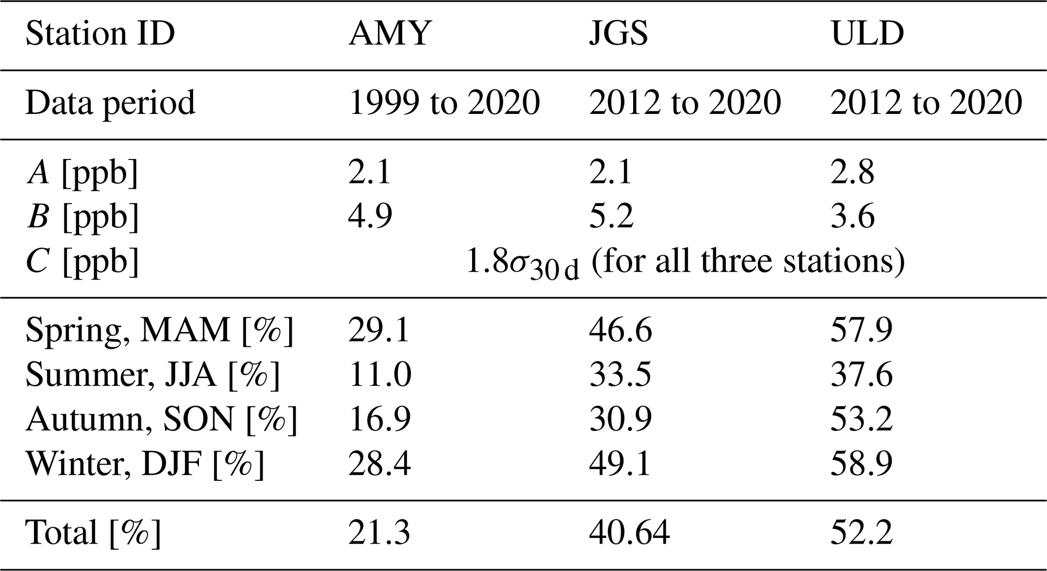
HS represents CH₄ hourly standard deviation, and HA is CH₄ hourly means and t represents time in hours. In Step (3), t is the middle of the time window. A, B, and C are criteria determined empirically for each step, as given in Table 2. C is the standard deviation of 30 d moving average multiplied by α, and here 1.8σ_30 d is applied to all three stations as C.

Even though the data were selected by steps (1) and (2), high CH₄ levels remained because of long-lasting stagnant conditions (e.g. over 6 d). Therefore, we also apply step (3). This process retained 21 %–52 % of the data at each station, which were defined as L3 hourly on observations (Fig. S2 in the Supplement). To get L3 daily/monthly data, the method developed by Thoning et al. (1989) was used to fit smooth curves to the daily averages computed by L3 hourly data. The methods reduce noise induced by synoptic-scale atmospheric variability, fill measurement gaps, and are used to represent the regional baseline. The details are described in Sect. S2 in the Supplement. Finally, we can get the L3 daily data, L3 monthly data, long-term trend and seasonal amplitude after applying the method by Thoning et al. (1989). The detailed definitions are in Sect. S3 in the Supplement.

CH₄ data were produced under the same conditions for all three stations; however, ULD was affected by emissions from a garbage incinerator until December 2016, while AMY was affected by a malfunction of the drying system for 26 August–9 September 2016. The garbage incinerator was moved to the northeast part of the island in December 2016. Therefore, we compared data from the three stations from 2016 to 2020, excluding the periods mentioned above.

In Sect. 3.5, for comparison of our station annual/monthly mean and seasonal amplitude to those parameters calculated from other Asian stations, WLG and RYO, we downloaded daily data for these stations from the World Data Centre for Greenhouse Gases (http://gaw.kishou.go.jp, last access: 29 May 2023). We applied the Thoning et al. (1989) method to each daily data set to get monthly mean and seasonal amplitude to compare. Annual means are averaged by monthly means, while annual growths are derived from the difference of consecutive annual means.

2.5 Flask-air data

Long-term data on CH₄ and its isotopes (δ¹³C in CH₄, hereafter ${\mathit{\delta }}^{\mathrm{13}}{\mathrm{C}}_{\left({\mathrm{CH}}_{\mathrm{4}}\right)}$ were collected at TAP, 28 km away from AMY. Samples were collected weekly between 12:00 and 18:00 (South Korea local time), when boundary layer height (BLH) was maximum to reduce local impacts. The pair of flask-air samples (2 L each flask, borosilicate glass with Teflon O-ring sealed stopcocks) was flushed for 10 min at 5–6 L min⁻¹ then pressurized to 0.38 bar in less than 1 min using a semi-automated portable sampler. The collected samples were sent to Boulder, Colorado, for measurement of CH₄ at NOAA and to INSTAAR (Institute of Arctic and Alpine Research, University of Colorado) for ${\mathit{\delta }}^{\mathrm{13}}{\mathrm{C}}_{\left({\mathrm{CH}}_{\mathrm{4}}\right)}$ analysis (Miller et al., 2002). Samples were analyzed from 1990 for CH₄ and from 2000 for ${\mathit{\delta }}^{\mathrm{13}}{\mathrm{C}}_{\left({\mathrm{CH}}_{\mathrm{4}}\right)}$. Since TAP and AMY are only 28 km apart, their data are representative of the same region under large synoptic conditions (Fig. S3 in the Supplement), especially for well-mixed air. These data were thus used to trace the changes in the surrounding environment in East Asia (Sect. 3.5). AMY started flask sampling for CH₄ and ${\mathit{\delta }}^{\mathrm{13}}{\mathrm{C}}_{\left({\mathrm{CH}}_{\mathrm{4}}\right)}$ in December 2013, with the same method as TAP, and these data were used only for characterization of CH₄ at AMY in Sect. 3.4.3.

To understand the regional source signature of excess CH₄ and to consider background atmospheric variations, Miller–Tans plot are used with flask sample data (Miller & Tans, 2003).

$${\mathit{\delta }}_{\text{obs}}{C}_{\text{obs}}-{\mathit{\delta }}_{\text{bg}}{C}_{\text{bg}}={\mathit{\delta }}_{\mathrm{s}}(C_{\text{obs}}-C_{\text{bg}})$$

Here, C and δ refer to CH₄ and ${\mathit{\delta }}^{\mathrm{13}}{\mathrm{C}}_{\left({\mathrm{CH}}_{\mathrm{4}}\right)}$, and the subscripts bg, obs, and s refer to background, observed, and source values. Therefore, by plotting δ_obsC_obs−δ_bgC_bg (y) against C_obs−C_bg (x), δ_s indicates the slope of the linear regression represents the source ${\mathit{\delta }}^{\mathrm{13}}{\mathrm{C}}_{\left({\mathrm{CH}}_{\mathrm{4}}\right)}$ signature. Observed ${\mathit{\delta }}^{\mathrm{13}}{\mathrm{C}}_{\left({\mathrm{CH}}_{\mathrm{4}}\right)}$ values are selected by cluster analysis (Sect. 2.6). For background data, we downloaded data of CH₄ and ${\mathit{\delta }}^{\mathrm{13}}{\mathrm{C}}_{\left({\mathrm{CH}}_{\mathrm{4}}\right)}$ observed at Mauna Loa (https://gml.noaa.gov/dv/data, last access: March 2022).

2.6 Hybrid Single-Particle Lagrangian Integrated Trajectory model (HYSPLIT) cluster analysis

We downloaded and installed the HYSPLIT for Windows and used the built-in algorithm. HYSPLIT trajectories were calculated using the Global Data Assimilation and Prediction System (GDAPS) at a horizontal resolution of 25 km to determine the origin of air masses transported to TAP during 2006–2020. The back trajectories were calculated for 96 h periods at 3 h intervals, with 500 m altitude matching the time of each flask-air sample. Based on a cluster analysis, northern China (CN) accounted for 27 % of all air masses; these originated in Russia and traveled through Mongolia and northeast China. Southern China (CS) accounted for 6 %; these air masses originated from the East China Sea and the southern part of China. Air masses from the Korean Peninsula local (KL) sector reflected emissions from the Korean Peninsula and Japan, accounting for 17 % of the total air masses. Among clusters, 25 % of samples are derived from under stagnant conditions, which might be affected by local pollution. Therefore, we did not consider this sector. Other sectors were also analyzed, but there were no significant or representative emission signals from potential source strength (Sect. 2.7), so they are not reported herein.

2.7 Potential source strength (PSS) analysis

To identify and illustrate the potential source distributions for regional pollution, we calculated the PSS using the trajectory statistics approach, which has often been applied to estimate the potential source areas of greenhouse gases (Reimann et al., 2004, 2008; Li et al., 2017). The trajectory statistics approach was introduced first by Seibert et al. (1994). The underlying assumption of the method is that elevated atmospheric levels at an observation site are proportionally related to the air mass residence time on a specific grid cell over which the observed air mass has been passing. Thus, this method simply calculates the air mass residence time-weighted mean abundance (here, units of mole fraction) for target compounds (CH₄ in this study) in the domain with 0.5 × 0.5 grids using the following formula (Eq. 2):

$$\begin{array}{}\text{(2)}& \stackrel{\mathrm{‾}}{C_{(i,j)}}={\displaystyle \frac{{\sum }_{a=\mathrm{1}}^M{T}_{(i,j,a)}{C}_a}{{\sum }_{a=\mathrm{1}}^M{T}_{(i,j,a)}}},\end{array}$$

where C_(i,j) represents the potential source strength of the grid cell i and j as a potential source region of the target compound (CH₄), a is the index of the trajectory, M is the total number of trajectories that passed through cell i,j, C_a is the enhanced mole fraction (difference from background mole fractions described in Sect. 3.2) measured during the arrival of trajectory a, and $T_{(i,j,a)}$ is the residence time of trajectory a spent over grid cell i and j, calculated using the method described by Poirot and Wishinski (1986) with the following formula (Eq. 3):

$$\begin{array}{}\text{(3)}& T_{(i,j,a)}={\sum }_{n=\mathrm{1}}^N{\displaystyle \frac{S_{(i,j,n,a)}}{V_{(n,a)}}},\end{array}$$

where $S_{(i,j,n,a)}$ is the length of that portion of the nth segment of a back-trajectory which falls over grid cell i and j. V_(n,a) is the average speed of the air parcel as it travels along the nth segment of the a back-trajectory using the HYSPLIT model. To ensure trajectory reliability, we used only 4 d (96 h) back-trajectories at an altitude of 500 m above mean sea level. To consider the influence of air masses on emissions at ground level, air masses passing above the boundary layer height (BLH) were excluded. BLH is obtained from the HYSPLIT model. To exclude the influence of emission sources surrounding AMY, enhanced CH₄ data with wind speeds lower than 2 m s⁻¹ were omitted from the PSS analysis. When we compare our PSS results from AMY, JGS, and ULD using CH_4xs data from 2016 to 2020, they showed similar source regions, while the coverage and CH_4xs are slightly different (Fig. S4 in the Supplement).

3 Results and discussion

3.1 Measurement uncertainty

Observed CH₄ is influenced by natural atmospheric variability and measurement procedures. Natural atmospheric variability can be represented as the standard deviation of all measurements contributing to a time average, after accounting for experimental noise. The measurement uncertainty is critical to provide information on data quality so that users can understand the limitations and reliability of measurement. According to previous studies, the total measurement uncertainty consists of multiple uncertainty components (Andrews et al., 2014, Verhulst et al., 2017). For the KMA network, a measurement uncertainty of approximately 0.11 ppm has been calculated for CO₂ with limited but practical components (Lee et al., 2019). Using the same method used for CO₂, we calculated a practical realistic measurement uncertainty for CH₄ in the KMA network (Eq. 4). Based on the measurement of target cylinders and a co-located comparison of measurements at AMY and JGS, we assumed systematic biases to be negligible (http://empa.ch/web/s503/wcc-empa, last access: January 2022).

$$\begin{array}{}\text{(4)}& (U_{\mathrm{T}}{)}^{\mathrm{2}}=(U_{\text{h2o}}{)}^{\mathrm{2}}+(U_{\mathrm{p}}{)}^{\mathrm{2}}+(U_{\mathrm{r}}{)}^{\mathrm{2}}+(U_{\text{scale}}{)}^{\mathrm{2}},\end{array}$$

where U_T is the total measurement uncertainty in the reported dry-air mole fractions, U_h2o is the uncertainty from the drying system, U_p is repeatability, U_r is reproducibility defined as a drift occurring between calibration episodes, and U_scale is the uncertainty of propagating the WMO-X2004A CH₄ scale to working standard gases.

U_h2o was computed from the differences in H₂O (%) between the ambient airstream through the drying system and standard gases injected directly, bypassing the drying system. An ideal measurement would be through the analysis of the standard gases and air samples after they pass through the same drying system (Crotwell et al., 2019). However, our drying efficiency was not constant, so we injected standard gases directly as a reference value of H₂O. Therefore we considered the CH₄ dilution offsets between working standards and sample air while estimating the uncertainty with a similar method using Eq. (1) in Sect. 2.3. Hourly CH₄ dilution maximum offsets are up to 0.009 ppb at AMY, 0.006 ppb at JGS, and 0.009 ppb at ULD from 2016 to 2020. This uncertainty term was smallest (0.006 to 0.008 ppb) among all uncertainty factors in the KMA network, indicating the sampled air has negligible biases through our drying system.

$$\begin{array}{}\text{(5)}& U_x=\sqrt{{\displaystyle \frac{{\sum }_{i=\mathrm{1}}^N(x_i{)}^{\mathrm{2}}}{N}}},\end{array}$$

where U_x represents U_h2o, x is the hourly CH₄ dilution offsets from Eq. (1), and N is the total number of hourly mean values. U_h2o is tabulated for each station in Table 3.

Table 3 Uncertainty estimates for measurements of CH₄ at each station from 2016 to 2020. Units are parts per billion (ppb). All terms are 68 % confidence intervals.

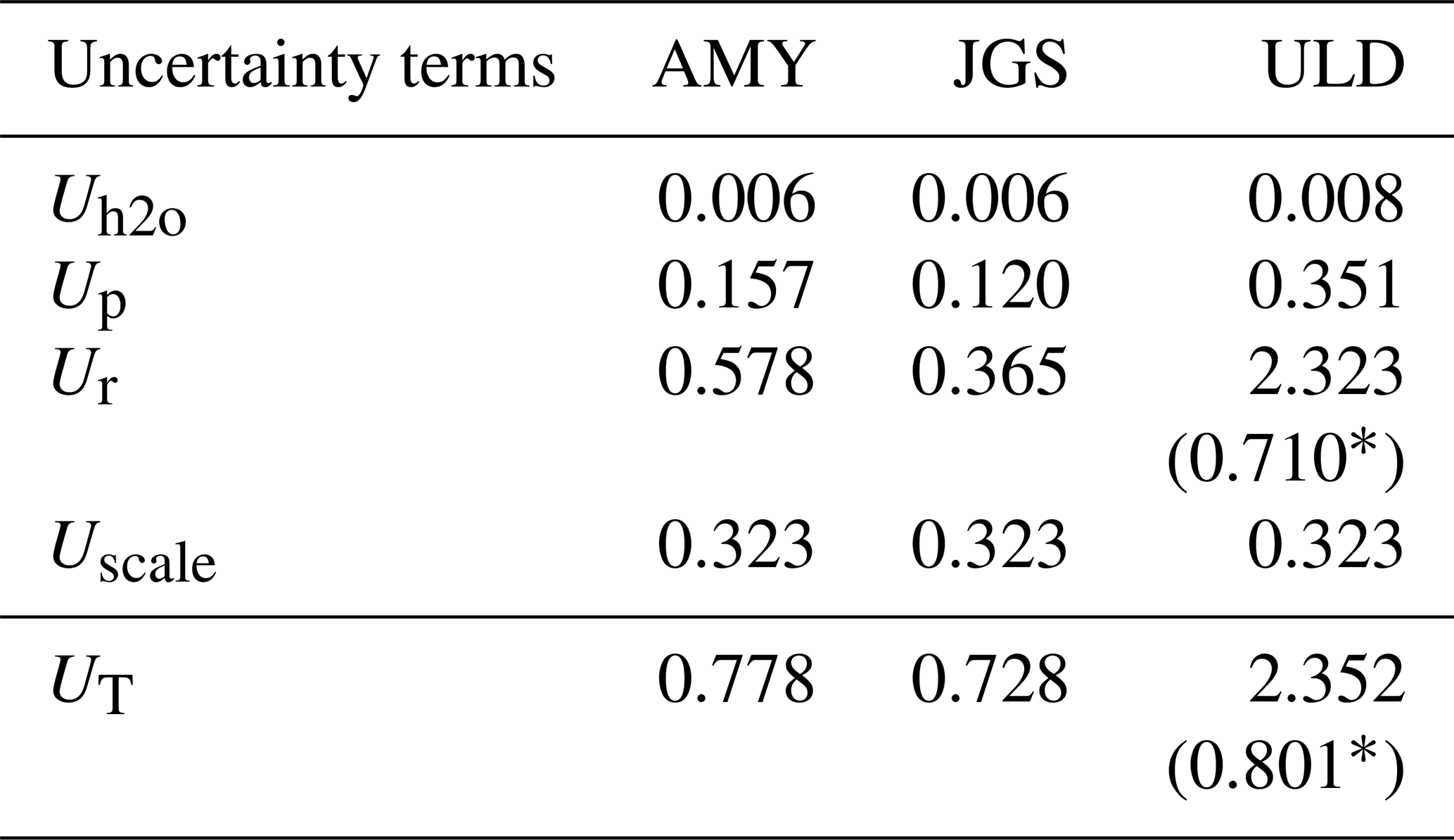
^∗ This value was calculated excluding the period with 1-month calibration frequency

We calculated U_r as the standard deviation of all drift using Eq. (5), where U_x represents U_r, x_i is the drift occurring between calibration episodes, and N is the total number of data. They are tabulated with other uncertainty terms by site in Table 3. We determined U_r as the differences in CH₄ measured from cylinders with subsequent calibrations after 2 weeks. It ranged from −0.9 to 2 ppb at AMY and from −1.25 to 0.84 ppb at JGS. ULD had a 2-week calibration period, which changed to 1 month from 18 May 2017 to 11 November 2019. During this period of 1-month calibration frequency, U_r increased to a maximum of 4 ppb, which is greater than the WMO/GAW compatibility goal of ± 2 ppb. After conducting the reproducibility test in November 2019, the calibration frequency decreased to 5 d. Therefore, U_r at ULD was separated into two groups including or excluding the period with a longer calibration period (with asterisk in Table 3). When we only considered the period with a higher calibration frequency, the uncertainty at ULD was similar to that at other stations. This means that U_r is the largest component of measurement uncertainty and that U_T can be decreased using an appropriate calibration strategy.

U_p was determined from the standard deviations of working standard measurements, as described in Sect. 2.3, and expressed by a pooled standard deviation (Eq. 6).

$$\begin{array}{}\text{(6)}& U_{\mathrm{p}}=\sqrt{{\displaystyle \frac{{\sum }_{i=\mathrm{1}}^N{N}_i\times {S_i}^{\mathrm{2}}}{N_i-N_{\mathrm{t}}}}},\end{array}$$

where S_i is the standard deviation of 10 min averages of working standard measurements, N_i the index number of a measurement during 10 min (based on 5 s intervals), and N_t is the total number of calibrations during the period. S_i was less than 0.882 ppb at AMY, 0.603 ppb at JGS, and 0.688 ppb at ULD. The pooled standard deviations (U_p) are shown in Table 3.

According to Zhao et al. (2006), the uncertainty of working standards can be calculated by the propagation error arising from the uncertainty of primaries with a maximum propagation coefficient (γ = 1) and repeatability. Similarly, U_scale for working standards is determined by (Eq. 7)

$$\begin{array}{}\text{(7)}& U_{\text{scale}}=\sqrt{U_p^{\mathrm{2}}+U_{\text{lab}}^{\mathrm{2}}},\end{array}$$

where U_lab is the uncertainty of laboratory standards, which CCL (NOAA/GML) certified. Here, U_lab has the same value as the uncertainty of secondary standards, 0.3 ppb with a confidence interval of 68 %, based on calibration of the secondary standards against the primary standards (http://gml.noaa.gov/ccl/ch4_scale.html, last access: January 2022). These values were the same for all stations since they were calibrated by a central lab at NIMS in Jeju. Therefore, U_p is the repeatability at the central lab since we propagated the standard scale through the same analyzer and setup for atmospheric monitoring. This value was always less than 0.12 ppb.

For AMY, the difference from the CCL in the RR test with the analysis of the same cylinder was from −0.3 to 1.3 ppb using a GC-FID in 2010. Therefore, we considered the largest value of 1.3 ppb as the measurement uncertainty from 1999 to February 2016 during the GC-FID measurement period.

Overall, the total measurement uncertainty was calculated to be from 0.728 to 0.801 ppb. These values were similar to those reported by CRDS measurements (< 1 ppb) (Winderlich et al., 2010; Andrews et al., 2014, Verhulst et al., 2017). In the future, quoted uncertainties could be greater, owing to the inclusion of more error sources, while reproducibility may improve with a different calibration strategy.

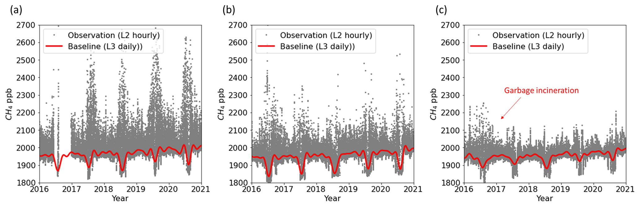
Figure 2 L2 hourly (grey scatters, observation) and fitted L3 daily data (red line, baseline) at (a) AMY, (b) JGS, and (c) ULD from 2016 to 2020.

3.2 Local/regional effects on observed CH₄

The enhancement of CH₄ relative to the regional background can help evaluate local/regional additions to CH₄, with the excess signal defined as (Eq. 8)

$$\begin{array}{}\text{(8)}& {\mathrm{CH}}_{\mathrm{4}\mathrm{xs}}={\mathrm{CH}}_{\mathrm{4}\mathrm{obs}}-{\mathrm{CH}}_{\mathrm{4}\mathrm{bg}},\end{array}$$

where CH_4obs is L2 hourly data (before filtering), and CH_4bg indicates the regional background at a site as determined by the smoothed curve fitted to L3 daily data (Sect. 2.4.2). CH_4xs was greatest in the order AMY (55.3 ± 37.7 ppb) > JGS (24.1 ± 10.2 ppb) > ULD (7.4 ± 3.9 ppb) from 2016 to 2020. For ULD, we excluded data collected in 2016 as they were affected by the garbage incinerator next to the station (Sect. 2.4, Fig. 2c). All stations showed largest CH_4xs in summer (June, July, August), with 109.6 ± 23.8 ppb at AMY, 37.0 ± 2.1 ppb at JGS, and 12.2 ± 3.7 ppb at ULD. Conversely, the smallest values were observed as 25.6 ± 2.4 ppb at AMY and 18.8 ± 4.1 ppb at JGS in spring (March, April, May), while the lowest value of 7.5 ± 0.4 ppb at ULD was observed in winter (December, January, February). The baseline selection conditions listed in Table 2 also supported this result. The selected baseline data accounted for only 11 %–37.6 % of summer data at all stations, indicating that CH₄ levels were elevated in summer. In winter and spring, we could better capture well-mixed air compared with other seasons (28.4 %–58.9 %) because of the strong westerly wind with the Siberian high.

To understand the influence of local surface wind on observed CH₄, bivariate polar plots were used for 2018, the year least affected by typhoons compared to other years.

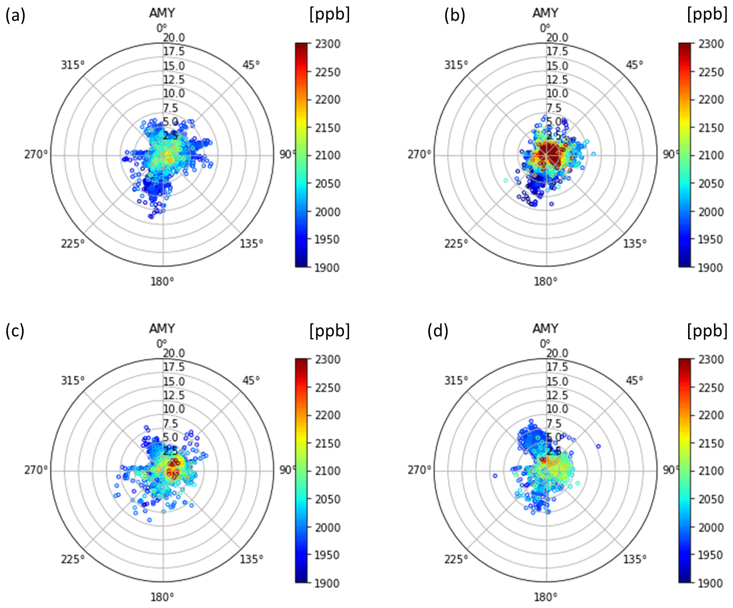
Figure 3 Bivariate polar plots for observed CH₄ (L2 hourly) in spring (a), summer (b), autumn (c), and winter (d) at AMY in 2018.

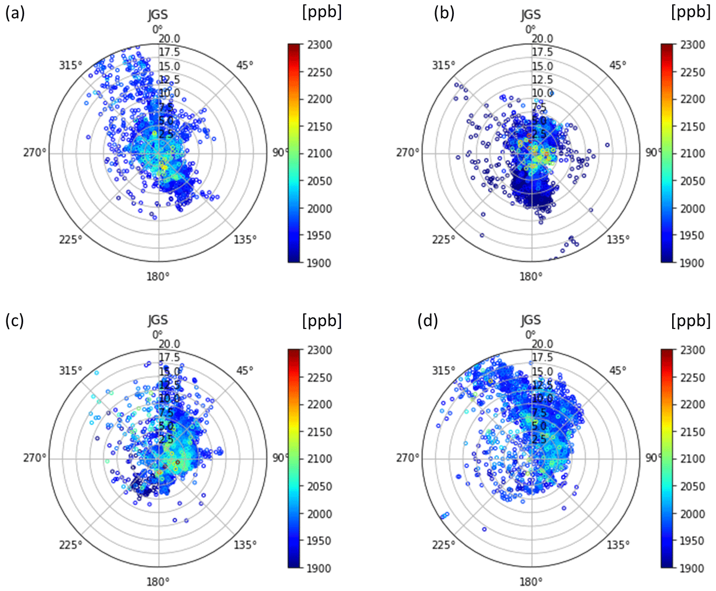
Figure 4 Bivariate polar plots for observed CH₄ (L2 hourly) in spring (a), summer (b), autumn (c), and winter (d) at JGS in 2018.

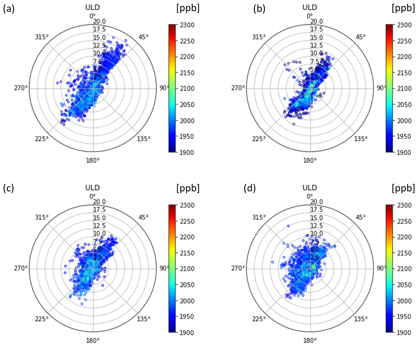
Figure 5 Bivariate polar plots for observed CH₄ (L2 hourly) in spring (a), summer (b), autumn (c), and winter (d) at ULD in 2018.

These plots express the dependence of all hourly CH₄ (L2 hourly data before selecting baseline) on wind direction and speed (Figs. 3–5). The wind data were derived from an AWS, as described in Sect. 2.1.

At AMY, when wind speed was consistently < 3 m s⁻¹, CH₄ was elevated during all seasons. Especially in summer, it showed strong signals when the wind direction was between 45 and 135^∘ (from land). A similar observation was made in other seasons, possibly indicating that this was related to local influences such as from rice paddies. The dominant wind direction was southwest in summer and northwest in winter. Even though lower CH₄ levels were captured regardless of wind direction with increased wind speed, CH_4xs was still higher than that at the other two stations. Therefore, AMY could be affected not only by local activities but also by distant emissions.

JGS experienced the strongest winds among the three stations in all seasons (maximum 27.5 m s⁻¹). Strong northwesterly wind (open sea) occurred in spring and winter, and air masses from the northeast (Korean Peninsula inland) were noted during autumn and from the south (open sea) during summer. CH₄ was lower than at AMY, with strong signals observed in all seasons under different criteria. Higher CH₄ levels occurred because of winds from the eastern part of JGS in autumn and summer when the wind speed decreased to less than 5 m s⁻¹. For spring and winter, strong signals were noted in the eastern and northern parts of JGS. Since JGS is located downwind from continental Asia and strong westerly winds occur in winter/spring because of the strong Siberian high, this signal might be related to activities not only in Asia but also in Jeju.

For ULD, the main wind directions were quite clearly from 0 to 90^∘ (30 %) and from 180 to 270^∘ (33 %), and wind speeds less than 5 m s⁻¹ occurred 72 % of the total time. High CH₄ episodes were mainly observed when the wind direction was between 180 and 225^∘, presumably affected by the southeastern part of the Korean Peninsula. This wind direction was very dominant in summer with a lower wind speed than that in other seasons.

Overall, atmospheric CH₄ observed by KMA WMO/GAW stations was affected not only by the local area but also by air masses from continental Asia, as indicated by the results from synoptic systems. Signals at AMY may be affected by local/regional activities, such as agriculture and livestock industries, owing to the relatively lower wind speeds; however, they still showed higher values compared with those of other stations when it captured well-mixed air. This indicates that AMY was affected not only by local sources but also by long-range transport of air masses originating from continental Asia. ULD showed lower CH₄ and was less affected by local impacts.

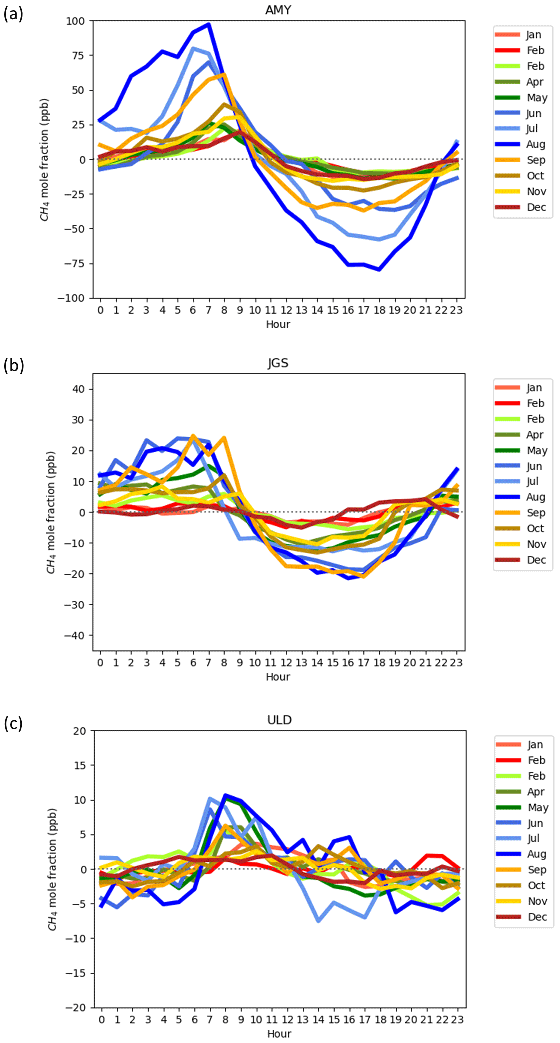
Figure 6 Mean diurnal variations of CH₄. Values show the average departure from the daily mean in each month at (a) AMY and (b) JGS from 2016 to 2020 and (c) at ULD from 2017 to 2020.

3.3 Average diurnal variation

Diurnal CH₄ variations were calculated as the average deviation from the daily mean in each month from L2 hourly data from 2016 to 2020 (recent 5 years) for AMY and JGS and from 2017 to 2020 for ULD (Fig. 6).

Among the three stations, the mean diurnal variation of all seasons was greatest at AMY (69.5 ± 49 ppb) and smallest at ULD (7.6 ± 4.2 ppb), while it was 24.7 ± 14.4 ppb at JGS. Daily variations in CH₄ are generally small at global-scale stations, so stations with a large seasonal cycle amplitude may be affected by local/regional sources (Aoki et al., 1992) and transport driven such as upslope/downslope air and land–sea breeze due to geographical reason.

AMY was surrounded by CH₄ sources as described in Sect. 2.1, while ULD had similar characteristics to global-scale stations that are less impacted by their local/regional environment. Similar to ULD, Mt. Waliguan station (3816 m), a representative global GAW station in Asia, also showed an amplitude of 5 to 10 ppb for the diurnal CH₄ cycle (Zhou et al. 2004; Fang et al., 2013).

Atmospheric CH₄ at AMY and JGS started to increase around midnight and peaked from 05:00 to 08:00 local time and then decreased with minimum value from 15:00 to 18:00. For ULD, the peaks were observed between 6:00 and 11:00, especially in summer, but there were no significant troughs. These variations at AMY and JGS were consistent with the changes in wind pattern and BLH. BLH was maximum near the middle of the day. At night, cooling caused by radiation loss at ground level leads to a stable boundary layer, leading to accumulation of CH₄ (Worthy et al., 1998; Higuchi et al., 2003). Both stations were also affected by land–sea breeze and received air from seaside during the daytime, which enhanced the diurnal variation. These patterns of CH₄ were similar to those of CO₂ observed by both stations (Lee et al., 2019) because of similar meteorological conditions. However, ULD is located on the slope of a mountain and is surrounded by complex terrain, thus being affected by certain winds from north to east and south to west, regardless of time and season. However, peak values only occurred during 6:00 to 11:00, which needs further study.

All stations showed the lowest amplitude in winter (December to February) and the largest amplitude in summer (June to August). AMY showed the largest diurnal amplitude (176.8 ± 74.6 ppb) in August among the three stations, which was almost 2.5 times greater than the annual mean value, with substantial variation among months. JGS and ULD showed the largest amplitude in August (43.4 ± 17.7 ppb) and July (17.2 ± 11.6 ppb), respectively. This indicated that the emission and meteorological impacts (e.g. maximized BLH and land–sea breeze) were strong in summer. AMY is close to rice paddies (110 km²), which are the major source of CH₄ in summer. JGS and ULD are not close to waterlogged paddies. However, high temperatures stimulate greater emissions from sources such as agriculture, livestock, and wetlands, thus affecting emissions at both stations. Similar to the observation made at AMY, previous studies have shown large variation in CH₄ emissions from the rice paddy area (196 ± 65 ppb) and wetland (∼ 150 ppb) during summer (Worthy et al. 1998; Fang et al., 2013).

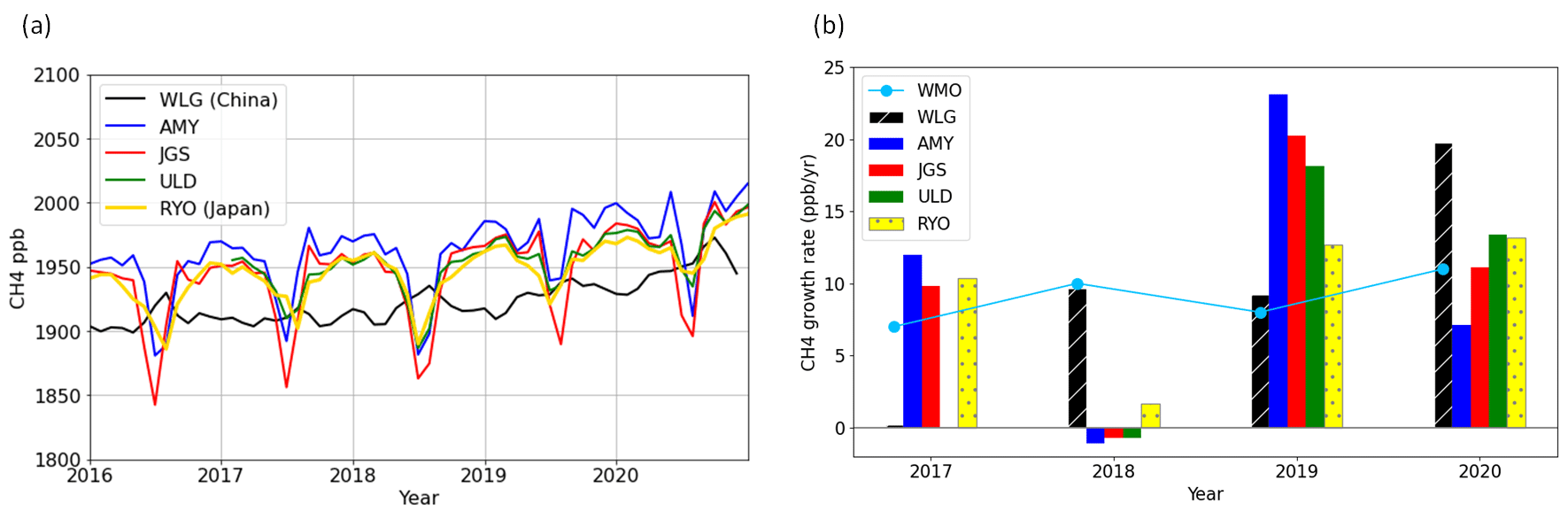
Figure 7 Time series of (a) monthly mean CH₄ and (b) annual growth rate at WLG, AMY, JGS, ULD, and RYO. The growth rate reported by WMO (Crotwell et al., 2022) is overlaid on (b), and this value is calculated as the change in annual mean from the previous year.

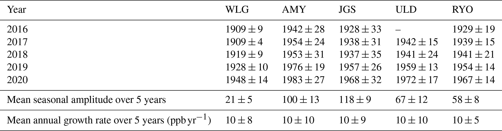
Table 4 Annual mean CH₄ with standard deviations from monthly mean from 2016 to 2020, mean seasonal amplitudes, and growth rates. Seasonal cycle amplitude during each calendar year was magnitude of the peak to trough of the detrended seasonal cycle (see Sect. 2.4.2). The growth rate is an annual increase (not de-seasonal) expressed as an absolute difference from previous year. Growth rate at ULD was only calculated from 2017 to 2020. Units are dry-air mole fractions (ppb).

3.4 Comparison with other East Asian stations: annual mean, seasonal amplitude, and growth rate

3.4.1 Annual mean

Time series of monthly mean CH₄ from KMA's three stations and the two other stations in East Asia are compared in Fig. 7a, and annual mean CH₄ is summarized in Table 4. Annual CH₄ mean was the highest at AMY and the lowest at WLG. The other stations showed similar levels of annual mean considering standard deviations. It was obvious that AMY was affected by local and regional activities, while WLG was affected by representative air masses of the Northern Hemisphere.

3.4.2 Seasonal amplitude

As described in Sect. 2.4, the seasonal amplitudes of CH₄ from 2016–2020 were calculated for three KMA stations and are compared with those values from WLG and RYO (Table 4). The seasonal amplitude is related to the seasonal atmospheric transport, for example, major wind direction and the combination of CH₄ surface flux distribution and chemical loss by reactions with OH and by soil loss. Seasonal amplitudes followed the order JGS > AMY > ULD > RYO > WLG (Table 4).

Since WLG is a global baseline station that is affected less by regional sources and sinks, the amplitude was smallest compared with the other regional stations. The amplitude of WLG was similar to that of other global stations such as Mauna Loa (30.6 ± 4.2 ppb) (Dlugokencky et al., 1995). Seasonal amplitudes at AMY and JGS are much greater than at the other three stations and even inland regional stations in China, such as Lin'an (77 ± 35 ppb) and Longfenshan (73 ± 8 ppb) (Fang et al., 2013). Minimum values at JGS are −14.8 ± 9.2 ppb lower than AMY minimum values, while the maximum values at both stations are similar. Li et al. (2018) reported that summer air mass was affected by large-scale low-level monsoonal circulation across the tropics in Jeju. A similar meteorological impact for CH₄ was reported at TAP (Dlugokencky et al., 1993). Even though transport and OH radicals can result in low CH₄ values at AMY, the station is also affected by nearby sources with enhanced emissions during summer. As we introduced in Sect. 2.1, AMY has large rice paddies and livestock industries within 50 km. During summer, high temperatures will enhance CH₄ emissions from these sources, leading to higher CH₄ than that at JGS (Kenea et al., 2021; Wang et al., 2021). Among regional stations, ULD and RYO may be less affected by regional flux because of their altitude, causing their amplitude to be greater than that of WLG but smaller than that of AMY or JGS.

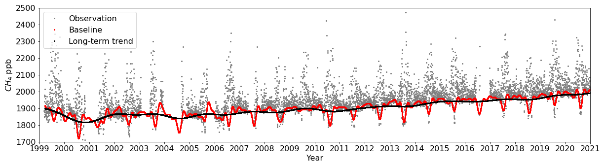
Figure 8 Time series of CH₄ (L2 daily, grey), baseline (L3 daily, red), and long-term trend (black) observed at AMY from 1999 to 2020.

Minimum values were observed in summer, while maximum values occurred in spring, autumn, or winter for different regional stations. In contrast, WLG showed maximum levels in summer and minimum values in winter/spring. Zhang et al. (2013) reported that regional/local sources and air masses from polluted regions influenced by industry, crop residue burning, and agriculture may affect CH₄ observations at WLG in summer.

3.4.3 Growth rate

The annual increasing/decreasing was calculated the difference in annual means from the previous year (Fig. 7b). When we analyzed the overall growth rate for five stations, mean values of annual growth rate from 2017 to 2020 were around 10 ppb yr⁻¹, which was similar to the WMO global mean (9 ± 2 ppb yr⁻¹). However, when yearly comparisons were made, WLG and the other four regional stations varied. Especially from 2016 to 2017, WLG showed no increase in CH₄, while CH₄ at other stations showed small or negative increases from 2017 to 2018. Normally the growth rate in CH₄ at WLG matches well with the WMO global increase/decrease trend (Fig. 7b). Wang et al. (2021) reported that CH₄ fluxes in Asia are influenced by the El Niño–Southern Oscillation (ENSO) and temperature; therefore, we compared the growth rate of CH₄ from four regional stations with both factors (Fig. S5 in the Supplement). This showed that the pattern of growth rate was quite similar to that of ENSO; however, even though the ENSO was negative (e.g., from 2017 to 2018) when surface temperature was high, the growth rate still increased. Miller–Tans plots show the signature of CH₄ increments into background air of Mauna Loa (Fig. S6 in the Supplement). And the slope was −52.3 ± 2.2 ‰ in winter and −53.7 ± 0.7 ‰ in summer at AMY during 2016 to 2020. These values are very similar to the observed values during the summer vegetation period when biogenic emissions are very active (−52.5 ± 1.9 ‰) in Europe (Varga et al., 2021), indicating that AMY was mainly affected by biogenic sources regardless of the season during this period. Throughout Asia, emissions from agriculture and waste account for over 50 % of the total, which is increasing every year (Jackson et al., 2020). Since climate variability, such as through the ENSO and temperature, drives biogenic sources, the CH₄-growth rates observed at regional stations in Asia are more sensitive to regional emissions than the global station.

3.4.4 Long-term records of CH₄ and its drivers in East Asia

In Fig. 8, the black line is the long-term CH₄ trend after the seasonal cycle has been removed (Sect. S3 in the Supplement). In 2009 there is no clear seasonal cycle because there was an instrumental malfunction in summer. The long-term trend at AMY was very similar to the global trend. From 1999 to 2005, the mean annual CH₄-growth rate (absolute differences from the previous year) was approximately −1.2 ppb yr⁻¹ at AMY, while the global value was 0.3 ppb yr⁻¹, and both values have increased since 2006. CH₄ increased by 3.3 ppb yr⁻¹ from 2006 to 2010 (global: 5.9 and by 8.3 ppb yr⁻¹ (global: 9 ppb yr⁻¹) from 2016 to 2020, indicating that the growth rate is accelerating.

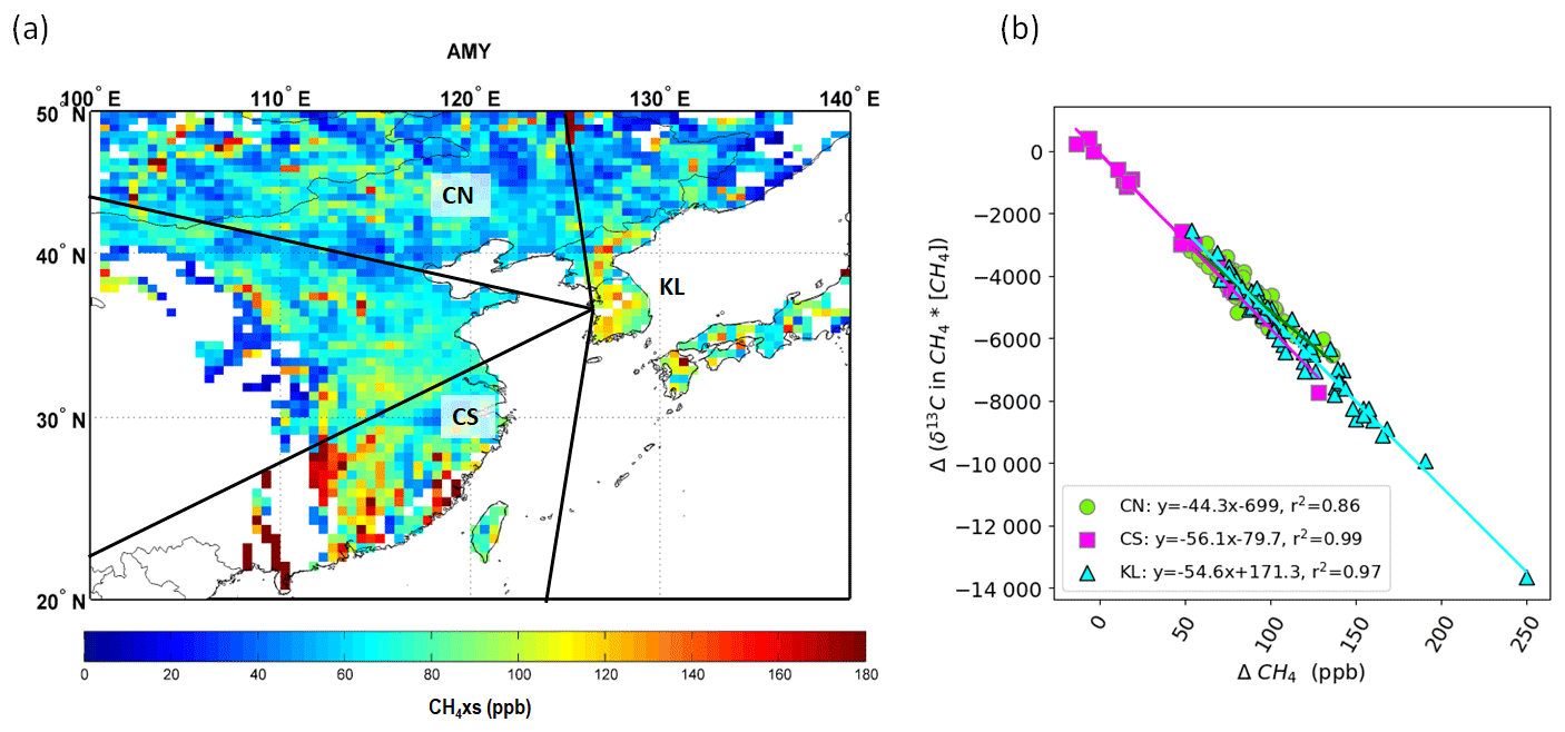
Figure 9 (a) PSS analysis with CH_4xs observed at AMY and (b) “Miller–Tans” plots from 2006 to 2020. Miller–Tans plots showing the source signature of methane increments (TAP) into background air (Mauna Loa).

To understand the source regions affected AMY CH₄ level, we analyzed PSS with hourly CH_4xs from 2006 to 2020. CH_4xs did not vary much and was 49 ± 74 ppb during 2006–2010 and 50 ± 70 ppb during 2016–2020. According to the PSS analysis, the major affected source regions were CN, CS, and KL sectors (Fig. 9a). Sources affecting CS and KL sectors were paddy and livestock fields, and the source affecting CN was reported to mainly be fossil fuel emissions (Zhang et al., 2011; Ito et al., 2022; Chen et al., 2022).

Through the HYSPLIT cluster analysis from 2006 to 2020, we categorized the TAP ${\mathit{\delta }}^{\mathrm{13}}{\mathrm{C}}_{\left({\mathrm{CH}}_{\mathrm{4}}\right)}$ data and selected the samples only affected by each source region, CN, CS, and KL sectors, respectively (Sect. 2.6). Using TAP ${\mathit{\delta }}^{\mathrm{13}}{\mathrm{C}}_{\left({\mathrm{CH}}_{\mathrm{4}}\right)}$ long-term data from 2006 to 2020 affected by CN, CS, and KL sectors, Miller–Tans plots indicated that emissions from CN were mainly related to fossil fuel or biomass burning (−44.3 ± 1.8 ‰), while CS (−56.1 ± 1.5 ‰) and KL sectors (−54.6 ± 1.2 ‰) were affected more by biogenic sources during 2006–2020 (Fig. 9b). Sherwood et al. (2017) reported unweighted global mean δ¹³C of −44.8 ± 10.7 ‰ from fossil fuel use, −26.2 ± 4 ‰ from biomass burning, and −61.7 ± 6.2 ‰ from microbial sources. Regionally, CH₄ emissions from wetlands in Siberia are at −69.9 ± 5.5 ‰, while in Hong Kong they were more enriched at −56.9 ± 3.8 ‰ (Ganesan et al.,2018). In northern China, a high coal emission area, a heavy CH₄ signal appears from −35 ‰ to −50 ‰ (Feinberg et al., 2018). Even though the uncertainty of isotopic source signature is quite large, CH₄ formed at high temperature such as through combustion is enriched in the heavier isotope, while CH₄ from wetland, rice paddies, and livestock is depleted. Therefore, our isotope analysis was well matched to reported source regions.

On the other hand, isotope signatures were shifted slightly in China (CN and CS), while for the Korean Peninsula local (KL) sector, they were steady in the uncertainty range from 2006 to 2020. When we analyze the Miller–Tans plots for every 5 years (Fig. S7 in the Supplement), for CN the slope was −38 ± 3 ‰ in 2006/10, but it became depleted −45 ± 2.4 ‰ in 2016/20, while it was enriched from −59.8 ± 1.5 ‰ to −51.9 ± 2.5 ‰ in CS. The KL sector showed quite constant values from −55 ± 1.6 to −54 ± 3.1 ‰ in the same period. This suggested that CH₄-growth rate in East Asia was affected by not only biogenic but also pyrogenic sources such as biomass burning and fossil fuel. The recent global accelerated increase in atmospheric CH₄ was more related to microbial sources such as agriculture and wetland (Lan et al., 2021; Basu et al., 2022).

Since the CH₄ emissions from agriculture and livestock accounted for 30 % and 36 % in China and South Korea, respectively, in 2020 (Crippa et al., 2022), CH₄ might be increased by temperature impacts on biogenic CH₄ sources. However, fast urbanization and increased energy consumption can also affect these regions. Especially the coal emissions decreased from 2010 in China (Liu et al., 2021), but the coal-to-gas policy led to an increase in natural gas consumption in China (Wang et al., 2022).

Overall, AMY and global growth rates were renewed in 2006 and accelerated during 2006–2020; the increasing trend could be linked to mixed biogenic and fossil fuel sources in East Asia while more biogenic sources globally.

4 Summary and conclusions

Among greenhouse gases, CH₄ emission reductions can be highly effective for short-term global warming mitigation because of its relatively short lifetime. However, its sources are diverse and yet to be evaluated completely through high-accuracy measurements. Our study analyzed CH₄ characteristics observed at regional KMA GAW stations, uncertainties related to its measurement, and changes in sources using long-term data in South Korea.

The KMA started monitoring atmospheric CH₄ in 1999 at AMY and expanded its network to the south and east parts of Korea at JGS and ULD in 2012 using a new system consisting of CRDS and a cryogenic drying system.

All three stations have similar measurement uncertainty from 2016 to 2020, in the range of 0.73–0.80 ppb. These uncertainties are similar to values reported in previous studies (less than 1 ppb). In addition, we confirmed reproducibility as the greatest contributor to measurement uncertainty; therefore, calibration strategies are the most critical component for reducing measurement uncertainty.

CH_4xs assessed relative to local background levels at each station was in the order AMY (55.3 ± 37.7 ppb) > JGS (24.1 ± 10.2 ppb) > ULD (7.4 ± 3.9 ppb). CH_4xs was greatest in summer and lowest in spring or winter. This result is consistent with wind direction and speed. In summer, local biogenic sources affected observed CH₄. Low wind speed enhanced CH_4xs, while lower CH₄ levels were observed when the stations experienced high wind speed. For AMY, even when CH₄ was measured in well-mixed air, its level was higher than that at other stations, indicating that it was affected not only by local sources but also by distant air masses from Asia. ULD showed representative CH₄ levels without local impacts. Diurnal variations were greatest at AMY and smallest at ULD and were affected by local sources and meteorological characteristics. The variation at ULD was 7.6 ± 4.2 ppb, similar to that at the WLG baseline station in China (5 to 10 ppb). All stations had large diurnal cycles in summer, indicating a strong influence of local biogenic sources at KMA sites.

When CH₄ seasonal cycle amplitudes measured at KMA stations were compared with those at other East Asian stations from 2016 to 2020, the following descending order was observed: JGS (103 ± 10) > AMY (85 ± 16) > ULD (58 ± 12) and RYO (57 ± 12) > WLG (30 ± 11). As discussed, since AMY reflected strong local influences not only in winter but also in summer, its seasonal amplitude was smaller than that of JGS. However, annual CH₄ mean was highest at AMY and lowest at WLG. The relative contributions of CH₄ source types to signals at regional stations in Asia are sensitive to temperature and ENSO. Based on analysis of ${\mathit{\delta }}^{\mathrm{13}}{\mathrm{C}}_{\left({\mathrm{CH}}_{\mathrm{4}}\right)}$ measurements, we established an increase in CH₄ from biogenic sources.

From the long-term analysis of CH₄ data at AMY, the average CH₄-growth rate was 3.3 ppb yr⁻¹ during 2006–2010, but it increased to 8.3 ppb yr⁻¹ in 2016–2020, similar to the global trend. Through the source distributions determined with our PSS analysis using CH_4xs data, CN, CS, and KL sectors were the main regions that affected atmospheric CH₄ observed at AMY. The isotope signature based on Miller–Tans plots at CN represented fossil fuel or burning activities, while CS and KL sectors represented biogenic sources during 2006–2020. However, we infer atmospheric CH₄ drivers changes in air masses arriving from the Chinese sector, CN and CS. For East Asia the increasing trend could be linked to mixed biogenic and fossil fuel sources, while globally the increase was dominated by microbial sources (e.g. agriculture and wetland). Through this study, we confirmed that long-term high-quality data can help understand changes in CH₄ emissions in East Asia. Also, further studies are necessary based on observations to understand sources changes in East Asia since there is a discrepancy between reported inventory and observations (Wang et al., 2022).