the Creative Commons Attribution 4.0 License.
the Creative Commons Attribution 4.0 License.
 | 26 Oct 2020
Observations of atmospheric 14CO2 at Anmyeondo GAW station, South Korea: implications for fossil fuel CO2 and emission ratios
Edward J. Dlugokencky
Jocelyn C. Turnbull
Sepyo Lee
Scott J. Lehman
John B. Miller
Gabrielle Pétron
Jeong-Sik Lim
Gang-Woong Lee
Sang-Sam Lee
Young-San Park
To understand the Korean Peninsula's carbon dioxide (CO2) emissions and sinks as well as those of the surrounding region, we used 70 flask-air samples collected during May 2014 to August 2016 at Anmyeondo (AMY; 36.53∘ N, 126.32∘ E; 46 m a.s.l.) World Meteorological Organization (WMO) Global Atmosphere Watch (GAW) station, located on the west coast of South Korea, for analysis of observed 14C in atmospheric CO2 as a tracer of fossil fuel CO2 contribution (Cff). Observed 14C ∕ C ratios in CO2 (reported as Δ values) at AMY varied from −59.5 ‰ to 23.1 ‰, with a measurement uncertainty of ±1.8 ‰. The derived mean value Cff of (9.7±7.8) µmol mol−1 (1σ) is greater than that found in earlier observations from Tae-Ahn Peninsula (TAP; 36.73∘ N, 126.13∘ E; 20 m a.s.l., 28 km away from AMY) of (4.4±5.7) µmol mol−1 from 2004 to 2010. The enhancement above background mole fractions of sulfur hexafluoride (Δx(SF6)) and carbon monoxide (Δx(CO)) correlate strongly with Cff (r>0.7) and appear to be good proxies for fossil fuel CO2 at regional and continental scales. Samples originating from the Asian continent had greater Δx(CO) : Cff(RCO) values, (29±8) to (36±2) nmol µmol−1, than in Korean Peninsula local air ((8±2) nmol µmol−1). Air masses originating in China showed (1.6±0.4) to (2.0±0.1) times greater RCO than a bottom-up inventory, suggesting that China's CO emissions are underestimated in the inventory, while observed RSF6 values are 2–3 times greater than inventories for both China and South Korea. However, RCO values derived from both inventories and observations have decreased relative to previous studies, indicating that combustion efficiency is increasing in both China and South Korea.
- Article
(401 KB) - Full-text XML
- Companion paper 1
- Companion paper 3
-
Supplement
(524 KB) - BibTeX
- EndNote


Carbon dioxide (CO2) is the principle cause of climate change in the industrial era and has been increasing in the atmosphere at (2.4 ± 0.4) µmol mol−1 a−1 in the past decade globally (where 0.4 is the standard deviation of annual growth rates; http://www.esrl.noaa.gov/gmd/ccgg/trends/, last access: 6 December 2019). This increase is by release of CO2 from fossil fuel combustion that has been demonstrated through 14C analysis of tree rings from the last two centuries (Stuiver and Quay, 1981; Suess, 1955; Tans et al., 1979). An atmospheric measurement program for the ratio 14C ∕ C in CO2 was initiated in the 1950s and 1960s (Rafter and Fergusson, 1957; Nydal and Lövseth, 1996). Observed 14C ∕ C ratios are reported in delta notation (Δ(14CO2)) as fractionation-corrected permil (or ‰) deviations from the absolute radiocarbon standard (Stuiver and Polach, 1977). Many studies show that the variation of Δ(14CO2) is an unbiased and now widely used tracer for CO2 emitted from fossil fuel combustion (Levin et al., 2003; Turnbull et al., 2006; Graven et al., 2009; Van der Laan et al., 2010; Miller et al., 2012). Therefore measurements of Δ(14CO2) are important to test the effectiveness of emission reduction strategies to mitigate the rapid atmospheric CO2 increase, since they can partition observed CO2 enhancements, Δx(CO2), into fossil fuel CO2 (Cff) and biological CO2 (Cbio) components with high confidence (Turnbull et al., 2006).
When trace gases are co-emitted with Cff, correlations of their enhancements with Cff improve understanding of the emission sources of both Cff and the co-emitted tracers. For example, CO and CH4 emission inventories are typically more uncertain than the fossil fuel CO2 emission inventory, since fossil fuel CO2 emissions related to complete combustion are generally well estimated, while emissions related to incomplete combustion and agricultural activities are poorly constrained (Kurokawa et al., 2013). Temporal changes in the observed emission ratio of a trace gas to Cff can be used to examine emission trends in the trace gas (Tohijima et al., 2014). Therefore the observed emission ratios of trace gases to Cff can be used to evaluate bottom-up inventories of various trace gases (e.g., Miller et al., 2012). Here, we used two trace gases, carbon monoxide (CO) and sulfur hexafluoride (SF6), for this analysis. CO is produced along with CO2 during incomplete combustion of fossil fuels and biomass. CO enhancements above background (Δx(CO)) correlate well with Cff and have been used as a fossil fuel tracer (Zondervan and Meijer, 1996; Gamnitzer et al., 2006; Turnbull et al., 2011a, b; Tohijima et al., 2014). SF6 is an entirely anthropogenic gas and is widely used as an arc quencher in high-voltage electrical equipment (Geller et al., 1997). At regional to continental scales, persistent small leaks to the atmosphere of SF6 are typically co-located with fossil fuel CO2 sources and allow SF6 to be used as an indirect Cff tracer, if the leaks are co-located with Cff emissions at the location and scale of interest (Turnbull et al., 2006; Rivier et al., 2006).
South Korea is a rapidly developing country with fast economic growth, and it is located next to China, which is the world's largest emitter of anthropogenic CO2 (Boden et al., 2017; Janssens-Maenhout et al., 2017). The first Δ(14CO2) measurements in South Korea were reported by Turnbull et al. (2011a) based on air samples collected during October 2004 to March 2010 at Tae-Ahn Peninsula (TAP; 36.73∘ N, 126.13∘ E; 20 m a.s.l.). This study showed that observed CO2 at this site was often influenced by Chinese emissions, and the observed ratio of Δx(CO) : Cff (RCO) was greater than expected from bottom-up inventories. However South Korean Δ(14CO2) data are still limited, and the ratio of the other trace gases to Cff is barely discussed.
Here we use whole-air samples collected in glass flasks during May 2014 to August 2016 at Anmyeondo (AMY; 36.53∘ N, 126.32∘ E; 46 m a.s.l.) World Meteorological Organization (WMO) Global Atmosphere Watch (GAW) station, located on the west coast of South Korea and about 28 km SSE of TAP, where the first study was conducted. We decompose observed CO2 enhancements into their fossil fuel and biological components at AMY to understand sources and sinks of CO2. We also implemented cluster analysis using the NOAA Hybrid Single Particle Lagrangian Integrated Trajectory Model (HYSPLIT) to calculate back-trajectories for sample times and dates. Based on clusters of trajectories from specific regions, trace gas enhancement to Cff ratios and correlation coefficients were analyzed, especially focusing on SF6 and CO, to determine the potential of alternative proxies to Δ(14CO2). Finally we compared our Δx(CO) : Cff ratio with ratios determined from bottom-up inventories (EDGARv4.3.2 and Korea's National Inventory Report in 2018) to evaluate reported CO emissions and how they have changed since 2010.
2.1 Sampling site and methods
The AMY GAW station is managed by the National Institute of Meteorological Sciences (NIMS) in the Korea Meteorological Administration (KMA). It has the longest record of continuous CO2 measurement in South Korea, beginning in 1999. It is located on the west coast of South Korea, about 130 km southwest of the megacity of Seoul, whose population was 9.8 million in 2017. The semiconductor industry and other industries exist within a 100 km radius of the station. Also, the largest thermal power plants fired by coal and heavy oil in South Korea are within 35 km to the northeast and southeast of the station. The closest town, around 30 km to the east of AMY, is well known for its livestock industries. Local economic activities are related to agriculture, e.g., production of rice paddies, sweet potatoes, and onions, and the area is also known for its leisure opportunities that increase traffic and tourists in summer, indicating the complexity of greenhouse gas sources around AMY. On the other hand, air masses often arrive at AMY from the west and south, which is exposed to the Yellow Sea. Therefore AMY observes enhanced CO2 compared to many other East Asian stations, due not only to numerous local sources but also the long-range transport of air masses from the Asian continent (Lee et al., 2019).
Two pairs of flask-air samples (four flasks in total, 2 L, borosilicate glass with Teflon O-ring sealed stopcocks) were collected about weekly from a 40 m tall tower at AMY, regardless of wind direction and speed from May 2014 to August 2016, generally between 14:00 and 16:00 local time (Table S1 in the Supplement), using a semi-automated portable sampler. A pair of flasks was flushed for 10 min at 5–6 L min−1 then pressurized to 0.38 bar in less than 1 min. A second pair is collected shortly after the first (within 20 min). The portable sampler was checked for leaks after pressurizing by observing the pressure gauge before closing the stopcocks. Batches of sampled flasks were shipped to Boulder, CO, USA, every 2 months.
A total of 70 sets were collected and analyzed at the National Oceanic and Atmospheric Administration/Global Monitoring Laboratory (NOAA/GML) for CO2, CO, and SF6 and for Δ(14CO2) by the University of Colorado Boulder, Institute of Arctic and Alpine Research (INSTAAR). NOAA/GML analyzed CO2 using a nondispersive infrared analyzer, SF6 using gas chromatography (GC) with electron capture detection, and CO using a vacuum UV resonance fluorescence instrument. All analyzers were calibrated with the appropriate WMO mole fraction scales (WMO-X2007 scale for CO2, WMO-X2014A scale for CO, and WMO-X2014 for SF6; https://www.esrl.noaa.gov/gmd/ccl/, last access: 4 December 2019). The measurement and analysis methods for these gases are described in detail (http://www.esrl.noaa.gov/gmd/ccgg/behind_the_scenes/measurementlab.html, last access: 4 December 2019). Measurement uncertainties for CO2 and SF6 are reported as 68 % confidential intervals. For CO2, it is 0.07 µmol mol−1 for all measurements used here. For SF6, it is 0.04 pmol mol−1. For CO, measurement uncertainty has not yet been formally evaluated but is estimated to be 1 nmol mol−1 (68 % confidence interval). All CO2, SF6, and CO data at AMY can be downloaded from ftp://aftp.cmdl.noaa.gov/data/trace_gases/ (last access: 1 September 2020). When we compare NOAA's CO2 measurements from flask air with quasi-continuous measurements by KMA at AMY, the difference was µmol mol−1 (mean ± 1σ), close to GAW's compatibility goal for CO2 (± 0.1 ppm for Northern Hemisphere measurements; Lee et al., 2019).
The analysis methods for Δ(14CO2) are described by Lehman et al. (2013). Measurement repeatability of Δ(14CO2) in aliquots of whole air extracted from surveillance cylinders is 1.8 ‰ (1σ), roughly equating to 1 µmol mol−1 Cff detection capability from the measurement uncertainty alone. The Δ(14CO2) data at AMY are tabulated in Table S1. Among four flasks, the air from two flasks, after analysis for greenhouse gas mole fractions, was combined and analyzed for Δ(14CO2).
2.2 Data analysis method using Δ(14CO2) data
2.2.1 Calculation of Cff and Cbio
As Turnbull et al. (2009) suggested, the observed CO2 (Cobs) at AMY can be defined as
where Cbg, Cff, and Cother are the background, recently added fossil fuel CO2, and the CO2 derived from the other sources.
According to Tans et al. (1993), the product of CO2 abundance and its isotopic ratio is conserved; the isotopic mass balance can be described as below:
where Δ is the Δ(14C) of each CO2 component of Eq. (1).
Therefore we can calculate fossil fuel CO2 by combining Eqs. (1) and (2) as
Fossil-fuel-derived CO2 contains no 14C because the half-life of 14C is (5700 ± 30) years (Godwin, 1962), while these fuels are hundreds of millions of years old. As we mentioned in Sect. 1, Δ(14CO2) is reported as a per mil (‰) deviation from the absolute radiocarbon reference standard corrected for fractionation and decay with a simplified form; ‰, where R(14C ∕ C) is the 14C ∕ C ratio. Therefore Δff is set at −1000 ‰ (Stuiver and Pollach, 1977). Background values (Δbg) in Eqs. (1) to (3) are determined from measurements from background air collected at Niwot Ridge, Colorado, a high altitude site at a similar latitude to AMY (NWR; 40.05∘ N, 105.58∘ W; 3526 m a.s.l.). Turnbull et al. (2011a) showed that the choice of background values did not significantly influence derived enhancements due to the large regional and local signal at TAP, 28 km from AMY. NWR Δ(14CO2) and other trace gas background values are selected using a flagging system to exclude polluted samples (Turnbull et al., 2007) and then fitted with a smooth curve following Thoning et al. (1989).
The second term of Eq. (3) is typically a small correction for the effect of other sources of CO2 that have Δ(14C) differing by a small amount from that of the atmospheric background, such as CO2 from the (1) nuclear power industry, (2) oceans, (3) photosynthesis, and (4) heterotrophic respiration.
(1) The nuclear power industry produces 14C that can influence the Cff calculation. South Korea has nuclear power plants along the east coast that may influence AMY air samples when air masses originated from the eastern part of South Korea (Fig. 1). It is also possible that Chinese nuclear plants could influence some samples. Here we did not make any correction for this since most nuclear installations in this region are pressurized water reactors, which produce mainly 14C in CH4 rather than CO2 (Graven and Gruber, 2011). (2) For the ocean, although there may also be a small contribution from oceanic carbon exchange across the Yellow Sea, we consider this effect small enough to ignore (Turnbull et al., 2011a). It was also demonstrated there is no significant bias from the oceans including the East China Sea (Song et al., 2018), even at coastal sites in the Northern Hemisphere (Turnbull et al., 2009). Larger scale ocean exchange and also stratospheric exchange affect both background and observed samples equally, so they can be ignored in the calculations. (3) For the photosynthetic terms, 14C in CO2 accounts for natural fractionation during uptake, so we also set this observed value to be the same as the background value. (4) Therefore we only consider heterotrophic respiration. For land regions, where most fossil fuel emissions occur, heterotrophic respiration could be a main contributor to the second term of Eq. (3) due to 14C disequilibrium potentially. When this value is ignored, Cff is consistently underestimated (Palstra et al., 2008; Riley et al., 2008; Hsueh et al., 2007; Turnbull et al., 2006). For this, corrections were estimated to be (−0.2 ± 0.1) µmol mol−1 during winter and (−0.5 ± 0.2) µmol mol−1 during summer (Turnbull et al., 2009, 2006).
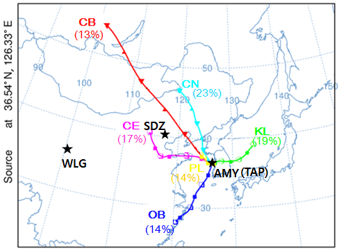
Figure 1A total of 70 air-parcel back-trajectories were calculated for 72 h periods at 3 h intervals from May 2014 to August 2016 using the HYSPLIT model in conjunction with KMA UM GDAPS data at a 25 km×25 km resolution. Station locations are as follows: WLG (Waliguan; 36.28∘ N, 100.9∘ E; 3816 m a.s.l.), SDZ (Shandianzi; 40.65∘ N, 117.12∘ E; 287 m a.s.l.), and AMY (Anmyeondo; 36.53∘ N, 126.32∘ E; 86 m a.s.l.). TAP (Tae-Ahn Peninsula; 36.73∘ N, 126.13∘ E; 20 m a.s.l.) is around 28 km northeast of AMY.
CO2 enhancements relative to baseline CO2 are defined as Δx(CO2), with the excess signal of Cobs minus Cbg in Eq. (1). Partitioning of Δx(CO2) into Cff and Cbio is calculated simply from the residual of the difference between observed Δx(CO2) and Cff.
2.2.2 The ratio of trace gas enhancement to Cff and its correlation
To obtain the correlation coefficient (r) between Cff and other trace gas enhancements () and the ratio of any trace gas to Cff (Rgas), we use reduced major axis (RMA) regression analysis (Sokal and Rohlf, 1981). The distributions of Rgas are normally broad and non-Gaussian, and RMA analysis is a relatively robust method of calculating the slope of two variables that show some causative relationship. Here, xbg was derived from NWR with the same method described in Sect. 2.2.1. The relevant equations are presented from Eqs. (S1) to (S3) in the Supplement. Results for each species are given in Table 1.
2.3 HYSPLIT cluster analysis
HYSPLIT trajectories were run using Unified Model-Global Data Assimilation and Prediction System (UM-GDAPS) weather data at a 25 km×25 km horizontal resolution to determine the regions that influence air mass transport to AMY. A total of 70 air-parcel back-trajectories were calculated for 72 h periods at 3 h intervals matching the time of each flask-air sample taken at AMY from May 2014 to August 2016. We assign the sampling altitude as 500 m, since it was demonstrated that HYSPLIT and other particle dispersion back-trajectory models (e.g., FLEXPART) are consistent at 500 m altitude (Li et al., 2014). Cluster analysis of the resulting 70 back-trajectories categorized six pathways through which air parcels arrive at AMY during the time period of interest.
Among the calculated back-trajectories, 67 % indicate air masses originating from the Asian continent. Back-trajectories of continental background air (CB) originating in Russia and Mongolia occurred 13 % of the time. A total of 23 % of the trajectories originated in and traveled through northeast China (CN). The CN region includes Inner Mongolia and Liaoning, one of the most populated regions in China, with 43.9 million people in 2012. These CN air masses arrive in South Korea after crossing through western North Korea. A total of 17 % of the trajectories are derived from central eastern China around the Shandong area (CE). The CE region contains Shandianzi (SDZ; 40.65∘ N, 117.12∘ E; 287 m a.s.l.), located next to the megacities of Beijing and Tianjin, which are some of China's highest CO2-emitting regions (Gregg et al., 2008). A total of 14 % have an ocean background (OB), derived from the East China Sea. Among them, a few of the trajectories passed over the eastern part of China (e.g., over Shanghai) at high altitude (1000 m). Flow from the Korean Peninsula also travels through heavily industrialized and/or metropolitan regions in South Korea (Korean Peninsula local air, KL; 19 %) and under stagnant conditions (polluted local region, PL; 14 %). Some of the KL air masses also passed over the East Sea and Japan.
Table 1Means and standard deviations of Cff (µmol mol−1), CO (nmol mol−1), and SF6 (pmol mol−1) (total N=50; without PL N=41). The correlations (r) and the ratio (Rgas) of enhancement between Cff values were determined by reduced major axis (RMA) regression analysis on each scatter plot to obtain regression slopes. The uncertainty of Rgas refers to Eq. (S2). When r is less than 0.7, Rgas was not included here. N is the number of data. The unit of RCO is nanomoles per micromole (nmol µmol−1), and for it is picomoles per micromole (pmol µmol−1). A plot of RCO and is shown in Fig. S1 in the Supplement. CB represents continental background, CN northeast China, CE central eastern China, OB ocean background, KL Korean Peninsula local air, and PL polluted local air mass.

3.1 Observed Δ(14CO2) and portioning of CO2 into Cff and Cbio
AMY Δ(14CO2) values are almost always lower than those observed at NWR, which we consider to be broadly representative of background values for the midlatitude Northern Hemisphere (Fig. 2). NWR Δ(14CO2), which is based on weekly air samples, was in the range 10.0 ‰ to 21.2 ‰, with an average (16.6 ± 3) ‰ (1σ, standard deviation) from May 2014 to August 2016. Waliguan (WLG; 36.28∘ N, 100.9∘ E; 3816 m a.s.l.), an Asian background GAW station in China, also showed similar Δ(14CO2) levels to NWR, with an average of (17.1 ± 6.8) ‰ in 2015 (Niu et al., 2016, measurement uncertainty ± 3 ‰, n=20). Δ(14CO2) at AMY varied from −59.5 ‰ to 23.1 ‰ and had a mean value of (−6.2 ± 18.8) ‰ (1σ, n=70) during the measurement period (Table S1). This was similar to results from observations at SDZ, which is located about 100 km northeast of Beijing, in the range of −53.0 ‰ to 32.6 ‰, with an average (−6.8 ± 21.1) ‰ (1σ, n=32) during September 2014 to December 2015 (Niu et al., 2016).

Figure 2Time series of (a) observed CO2 dry air mole fraction (open circles) and observed CO2 (Cobs) minus Cff calculated from Δ(14CO2) (closed circles). (b) Δ(14CO2) at AMY (black circles) and at NWR (Niwot Ridge; line), baseline data. (c) Time series of Cff and Cbio calculated from Δ(14CO2) (left) and the frequency distribution at AMY (right).
Calculated Cff at AMY ranges between −0.05 and 32.7 µmol mol−1, with an average of (9.7 ± 7.8) µmol mol−1 (1σ, n=70); high Cff was observed regardless of season (Fig. 2a). One negative Cff value of −0.05 µmol mol−1 was estimated due to greater AMY Δ(14CO2) than NWR on 30 July 2014. Although negative Cff values are nonphysical, this value is not significantly different from zero and is reasonable given that this air originated from the OB sector. The range of Cff in the AMY samples is similar to that observed at TAP from 2004 to 2010 (−1.6 to 42.9 µmol mol−1 Cff), but Cff is on average about twice as high at AMY as in the 2004 to 2010 TAP samples (mean (4.4 ± 5.7) µmol mol−1, n=202; Turnbull et al., 2011a). A more detailed comparison of results based on differences between samples derived from the Asian continent and Korean Peninsula local air is provided in Sect. 3.2.
Estimated Cbio, as defined in Sect. 2.2.1, varied from −18.1 to 15.7 µmol mol−1 (mean (0.9 ± 5.8) µmol mol−1) at AMY (Fig. 2c). Cbio showed a strong seasonal cycle, with the lowest values from July to September, when photosynthetic drawdown is expected to be strongest, in good agreement with the previous TAP study (Turnbull et al., 2011a). Even though Cbio was at times negative, mainly due to photosynthesis during summer, the largest positive Cbio was also observed in summer.
The largest Cff by season was observed in order of winter (DJF; (11.3 ± 7.6), n=14) > summer (JJA; (10.7 ± 9.2), n=11) > spring (MAM; (8.6 ± 8.0), n=22) > autumn (SON; (7.6 ± 5.6), n=17), in units of micromoles per mole (µmol mol−1). When we consider only positive contributions of Cbio samples, the order was summer ((4.6 ± 4.0), n=14) > autumn ((4.1 ± 2.5), n=9) > spring ((3.8 ± 2.6), n=13) > winter ((3.4 ± 2.5), n=11), in units of micromoles per mole (µmol mol−1).
Cff in summer was nearly as high as in winter. This is because lower wind speeds are observed at AMY during summer (Lee et al., 2019). When we analyzed seasonal boundary layer height for each sample by UM-GDAPS, it also showed a similar result; it was highest in winter (with a range from 150 to 1100 m) and lowest in summer (with a range from 100 to 500 m). This suggests that these high summer Cff values may reflect emission from local activities, which were described in Sect. 2.1, more than in other seasons.
The highest Cbio value was also observed in the summer in the PL sector. The PL sector showed that positive Cbio correlates with CH4, which is a tracer for agriculture when observed in TAP local air masses. Turnbull et al. (2011a) also showed similar results.
In winter, Cbio was relatively lower than in other seasons, while Cff was highest. During winter, AMY is mainly affected by long-range transport of air masses from China due to the Siberian High (Lee et al., 2019). Therefore air samples were less affected by local activities in winter, but Cbio still contributed almost 23 % to Δx(CO2). In the dry season (from October to March), forest fires, which contribute the largest portion of total CO2 emissions from open fires at the national scale, are concentrated in northeastern and southern China (Yin et al., 2019). The highest CO was observed in winter ((449.1 ± 244.1) nmol mol−1 (1σ) in winter while (236.8 ± 124.4) nmol mol−1 (1σ) in summer), which also supports biomass burning and biofuels as being large contributors to observed CO2 enhancements in winter. Turnbull et al. (2011a) also showed that 20 %–30 % of winter CO2 enhancements at TAP were likely contributed by biofuel combustion, along with plant, soil, human, and animal respiration.
Regardless of the source, we find that Cbio contributes substantially to atmospheric CO2 enhancements at AMY in air masses affected by local and long-range transport, so when only CO2 enhancements above background are compared to bottom-up inventories, it can create a bias due to Cbio contributions.
3.2 Cff comparison between Korean Peninsula local and Asian continent samples
To more clearly identify samples originating from the Asian continent (trajectory clusters CB, CN, CE, and OB) and Korean Peninsula local air (trajectory cluster KL) after cluster analysis of the 70 sets of measurements, we use wind speed data from the automatic weather system (AWS) installed at the same level as the air sample inlet at AMY. Among the data from CB, CN, CE, OB, and KL, when wind speed was less than 3 m s−1, we assumed that those samples could be affected by local pollution. PL was also ruled out since it was affected by local pollution under stagnant conditions. Therefore we use only 41 sets of observations for this analysis (Table 1).
Cff is highest in the order CE > CN > KL > CB > OB (Table 1). During the measurement period, the averages from the Asian continent (sectors CE and CN) were higher than KL without the baseline sector (CB and OB). The calculated mean Cff using only CE, CN, CB, and OB, which sample substantial outflow from the Asian continent, was (7.6 ± 3.9) µmol mol−1.
When we compared the KL samples ((8.6 ± 5.3) µmol mol−1) with those from Korean Peninsula local air masses observed at TAP ((8.5 ± 8.6) µmol mol−1, n=58; Turnbull et al., 2011a), mean Cff was quite similar (Fig. 3). However, when comparing the Cff values from CB air masses in this study and TAP long-range-transported samples (from China) (n=144; Turnbull et al., 2011a), Cff almost doubled from (2.6 ± 2.4) to (4.3 ± 2.1) µmol mol−1, even though they might be expected to have had similar air mass back-trajectories. We also compared the values at SDZ from 2009 to 2010 (Turnbull et al., 2011a) and in 2015 (Niu et al., 2016); they also increased, not only in the samples that were affected by Beijing and the North China Plain (SDZ-BN), which are comparably polluted, but also in the samples that were affected by northeast China (SDZ-NE). For SDZ-BN samples, Cff increased from (10 ± 1) to (16 ± 7.6) µmol mol−1 from 2009–2010 (n=32) to 2015 (n=32). The AMY samples from CE, which flow over Beijing, showed (11.2 ± 8.3) µmol mol−1 of Cff and were also slightly greater than the 2009–2010 SDZ-BN samples (Turnbull et al., 2011a). For SDZ-NE samples, Cff was (3 ± 7) µmol mol−1 in 2009 to 2010 and increased to (7.6 ± 6.8) µmol mol−1 in 2015. Since the SDZ-NE samples are affected by northeast China according to Turnbull et al. (2011a) and Niu et al. (2016), we also see CN that originated from northeast China (NE) and its mean value of Cff had increased around (10.6 ± 6.9) µmol mol−1 compared to those values in 2009 to 2010.
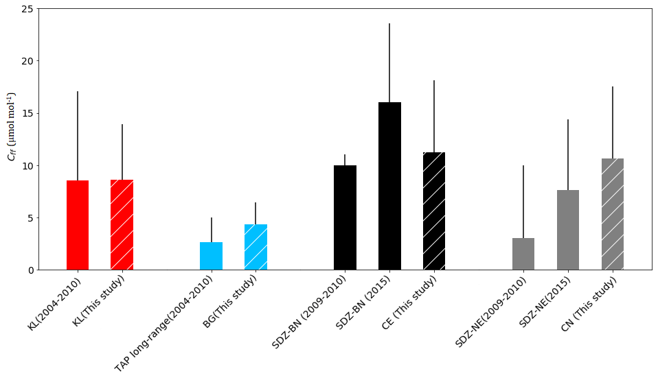
Figure 3Calculated Cff (µmol mol−1). Red bars are for KL, and blue bars are for South Korean long-range-transported samples (from China) (2004–2010 from Turnbull et al., 2011a). Black bars are for SDZ-BN samples that were affected by Beijing and the North China Plain. Gray bars for SDZ-NE indicate samples that were affected by regions northeast of SDZ. SDZ (2009–2010) is from Turnbull et al. (2011a), and SDZ (2015) is from Niu et al. (2016). Hatched red, blue, black, and gray bars are derived from this study during 2014 to 2016.
It has been suggested that inter-annual variability in observed mean Cff in South Korea could reflect changing fossil fuel CO2 emissions or could indicate inter-annual variability in the air mass trajectories of the (small) dataset of flask-air samples (Turnbull et al., 2011a). Even though the growth rate of Cff emission has been decreasing slowly in East Asia since 2010 due to emission reduction policies (Labzovskii et al., 2019), reported emissions increased 16.7 % in China and 1.8 % in South Korea from 2010 to 2016 (Janssens-Maenhout et al., 2017). This is broadly consistent with the flat trend in observed Cff in KL air masses and with the upward trend in Cff observed in air masses flowing out from Asia. Therefore it is possible that AMY mean Cff increased relative to the earlier TAP observations due to increased fossil fuel emissions from the Asian continent.
On the other hand, the values from this study showed large variability with small sample numbers due to a different sampling strategy, environment, and synoptic conditions such as boundary layer height at the sampling time from reference studies. Further study will be necessary to understand these increased values.
3.3 Correlation of Cff with SF6 and its emission ratios
We calculated correlation coefficients (r from Eq. S3) between SF6 and CO enhancements with Cff and their ratios from Eq. (S1) with the 50 samples that were described in Sect. 3.2 including the PL sector (n=9) and whose values are tabulated in Table 1.
The correlations of CO enhancements (Δx(CO)) with Cff were strong (r>0.7) in all sectors except PL, while SF6 enhancements (Δx(SF6)) correlated strongly with Cff (r>0.8) for CE and OB in outflow from the Asian continent and KL. RCO and were different between Korean Peninsula local air masses and outflows from the Asian continent. Here we discuss , and in Sect. 3.4 we discuss RCO in more detail.
For SF6, observed mean levels were high, in order of (KL, PL) > (CN, CE) > (OB, CB) (Table 1). SF6 values in KL and PL were higher than from the Asian continent, since South Korea has larger SF6 emissions than most countries (ranked fourth in 2010 according to EDGAR4.2.) because of liquid-crystal display (LCD) and electrical equipment production (Fang et al., 2014). Even though both KL and PL showed a higher SF6 mole fraction than outflows of the Asian continent, the correlation is different between KL and PL (Table 1). Under stagnant conditions, emitted SF6 is less diluted by mixing, so that in PL, Δx(SF6) correlated weakly with Cff. On the other hand, KL, CE, and OB showed strong correlations (r>0.8). Those three sectors are also larger SF6 sources compared to other regions, according to SF6 emission estimates for Asia (Fang et al., 2014). Because long-range transport allows time for mixing, SF6 and Cff emissions are effectively co-located at not only continental scales but also regional scales. Thus SF6 can be a good tracer of fossil fuel CO2 for those regions.
The correlation between Δx(SF6) and Cff was strong in CE, OB, and KL; however, is different between South Korea and outflow from the Asian continent (Fig. S2). In a previous study, observed was 0.02 to 0.03 pmol µmol−1 at NWR in 2004 (Turnbull et al., 2006). Here, the ratio was (0.19 ± 0.03) and (0.17 ± 0.03) pmol µmol−1 for CE and OB respectively. For KL, it was (0.66 ± 0.16) pmol µmol−1, indicating much larger ratios than in outflow from the Asian continent. Further, observed is 2 to 3 times greater for all air masses than predicted from bottom-up inventories based on a national scale. For this calculation, we use EDGAR4.3.2 for CO2 and EDGAR4.2 for SF6. We repeat the calculations for both CO2 and SF6 with Korea's National Inventory Report (KNIR; Greenhouse Gas Inventory and Research Center, 2018). Using SF6 for 2010 from EDGAR4.2, we obtain of 0.08 pmol µmol−1 for China, while for South Korea it was 0.14 pmol µmol−1. Especially for South Korea, this is much lower than the observed . When KL was compared to ratios calculated from KNIR (0.27 pmol µmol−1 for 2010 and 0.22 pmol µmol−1 for 2014), it was closer to observed than EDGAR but still underestimated (Figs. S3 and S2). This result suggests that the observed ratio could be used to re-evaluate the bottom-up inventories (Rivier et al., 2006), especially targeting the Asian continent. Even though KL showed greater uncertainty than CE and OB, it is still greater than bottom-up inventories, such as KNIR and EDGAR. Therefore it would be useful to obtain more data to try and derive a more robust estimate to evaluate SF6 emission inventories for South Korea.
3.4 Correlation of Cff with CO and its emission ratios
High CO was mainly observed in outflow from the Asian continent in order of CE > CN > PL > (CB, KL) > OB (Table 1). The order of CO is quite different to that of SF6. CO from KL and PL is lower than from outflow from the Asian continent, except for the OB sector, indicating that high CO can be a tracer of outflow from the Asian continent. Since CO is produced during incomplete combustion of fossil fuel and biomass, it is more closely related to fossil fuel CO2 emissions than the other trace gases. Therefore in most cases the correlation between CO and Cff was strong. RCO was very different between Korean Peninsula local air masses ((8 ± 2) nmol µmol−1) and those originating from the Asian continent ((29 ± 8) to (36 ± 2) nmol µmol−1), due to differences in combustion efficiencies and the use of catalytic converters. The higher continental emission ratios may also result from some contribution of biofuel combustion and agricultural burning in the Asian continent, which have significantly higher CO emission than fossil fuel combustion (Akagi et al., 2011). For example, for CB the CO level is similar to KL, while RCO is higher than KL with low Cff.
Typically CO shows seasonal variations, with lower values in summer due to the atmospheric chemical sink, OH. Among the samples, the samples collected in summer were mainly rejected through wind speed cutoff (less than 3 m s−1) since AMY has lower wind speed in summer (Lee et al., 2019). Only the OB sector includes four summer samples (of seven) because summer air masses are mainly from the southern part of the Yellow Sea (Lee et al., 2019). However, we assumed RCO is less affected by the summer sink, since only two Δx(CO) samples were negative for OB (Fig. S1), and RCO was consistent whether or not the negative Δx(CO) values were considered. To compare emission ratios derived from atmospheric observations with those from inventories for 2000 to 2012, we calculated the inventory emission ratio () as
where ECO and are total CO and fossil fuel CO2 emissions in gigagrams (Gg a−1, 109 g a−1) from the bottom-up national inventory. MX is the molar masses of CO and CO2 in grams per mole (g mol−1).
We use EDGAR4.3.2 (Janssens-Maenhout et al., 2017) and KNIR (Greenhouse Gas Inventory and Research Center, 2018) for inventory information for both CO and CO2.
The uncertainty of EDGAR4.3.2 fossil fuel CO2 emissions was reported as a 95 % confidence interval (Janssens-Maenhout et al., 2019), ± 5.4% for China and ± 3.6 % for South Korea (personal communication with Efisio Solazzo in the EDGAR team, 2020). The uncertainties of CO and SF6 emissions were not reported by EDGAR. For KNIR, the CO2 2016 emission uncertainty in the energy sector was ± 3% (Greenhouse Gas Inventory and Research Center, 2018). KNIR does not provide uncertainties for other emission sectors of CO2, nor for emissions of CO and SF6.
In Fig. 4 we confirm that the CO to Cff emission ratios (RCO) derived from both observations and inventories for China and South Korea are decreasing. Since Cff emissions appear to be flat (South Korea) or slightly increasing (China), this indicates that combustion efficiency and/or scrubbing of CO is improving.
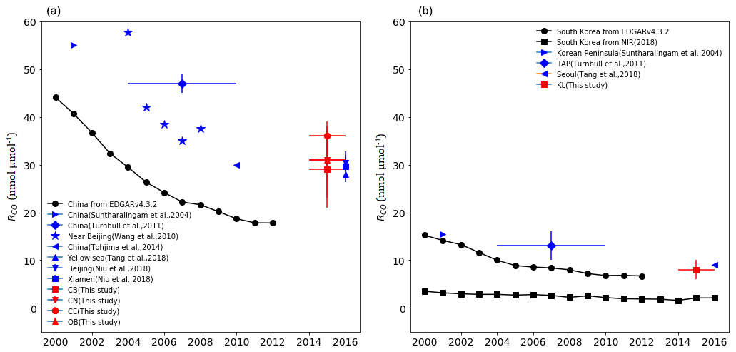
Figure 4RCO for China (a) and for South Korea (b). Black circles: EDGARv.4.3.2 emission inventory. Black squares: Korea's National Inventory Report (KNIR; Greenhouse Gas Inventory and Research Center, 2018). Blue symbols are from other studies (Suntharalingam et al., 2004; Wang et al., 2010; Turnbull et al., 2011a; Tohjima et al., 2014; Niu et al., 2018; Tang et al., 2018). Red symbols: this study. The y axis error bars represent the uncertainty in the slope according to Eq. (S2). The x axis error bars represent the period for the mean value.
For South Korea, EDGAR4.3.2 indicated that CO emissions from the energy sector (98 % to 99 % of total emission) decreased by 47 % between 1997 and 2012. South Korean fossil fuel CO2 emissions increased until 2011 and remained mostly constant from 2011 to 2016 ((603 901 ± 4315) Gg a−1 CO2) (Fig. S4). Therefore the decreased trend in the emission ratio seems to reflect recent decreases in CO emissions in South Korea. Turnbull et al. (2011a) determined an observed mean RCO of (13 ± 3) nmol µmol−1 during 2004 to 2010. Suntharalingam et al. (2004) estimated RCO 15.4 nmol µmol−1 for South Korea in 2001 from CO2 and CO airborne observations (Cff was not determined). Recently, the KORUS-AQ campaign, which was conducted over Seoul from May to June 2016, estimated RCO to be 9 nmol µmol−1 (Tang et al., 2018) based on CO2 and CO observations (Cff was not determined). Our study gives RCO of (8 ± 2) nmol µmol−1 for South Korea, slightly but not significantly lower than the KORUS-AQ result for Seoul. Different contributions of Cbio and Cff to total CO2 may have biased the RCO calculation when total CO2 was used in the KORUS-AQ study (e.g., Miller et al., 2012). The South Korean national RCO from EDGAR4.3.2 in 2012 was 6.7 nmol µmol−1, consistent with our observations. Using KNIR for 2016, we obtain RCO of 2.1 nmol µmol−1. KNIR suffers from a large number of missing CO emission sources compared to EDGAR, as indicated by their reported emissions, 638.3 and 2580.8 Gg a−1 in 2012, respectively (Fig. S5). For example, CO emissions recently derived from fugitive emissions and residential/other sectors increased to 14 % and 11.5 % of total emission respectively in EDGAR but were not reported in KNIR.
For China the inventories estimate that CO emissions from the energy sector, (96.5 ± 0.2) %, were almost constant through the 1990s and then increased during the early 2000s from industrial processes (8.8 % of total emissions in 2012). Fossil fuel CO2 emission in China also increased until 2013 and then stayed roughly constant at (10 461 890 ± 60 571) Gg a−1 according to EDGAR4.3.2. Thus even though both emissions show an increase from 2000 to 2016 for fossil fuel CO2 and to 2012 for CO, the emission ratio decreased (Figs. S4 and 4), which seems to indicate that combustion efficiency is improving. Many studies observed decreasing RCO in China from 2000 to 2010 (Turnbull et al., 2011a; Wang et al., 2010). Suntharalingam et al. (2004) reported that RCO was 55 nmol µmol−1 in 2001 (Cff was not determined). In the Beijing region, RCO decreased from 57.80 to 37.59 nmol µmol−1 during 2004 to 2008 (Wang et al., 2010). The overall RCO was (47 ± 2) nmol µmol−1 at SDZ for 2009–2010 and (44 ± 3) nmol µmol−1 in air masses that originated from the Asian continent from 2005 to 2009 (Turnbull et al., 2011a). Tohjima et al. (2014) explained that surface-based RCO decreased from 45 to 30 nmol µmol−1 in outflow air masses from China from 1998 to 2010. Fu et al. (2015) also observed RCO of 29 nmol µmol−1 over mainland China in 2009. In Beijing, which is located along the path of CE, it was (30.4 ± 1.6) nmol µmol−1 and (29.6 ± 3.2) nmol µmol−1 for Xiamen in 2016, which is in the OB sector (Niu et al., 2018). During KORUS-AQ in 2016, RCO of 28 nmol µmol−1 was observed over the Yellow Sea. Some of those studies did not differentiate Cff from the total CO2 enhancement, so, although RCO still includes uncertainties, it is continually decreasing.
In this study RCO is (29 ± 8), (31 ± 8), (36 ± 2), and (31 ± 4) nmol µmol−1 for CB, CN, CE, and OB, consistent with Tang et al. (2018) and Niu et al. (2018). On the other hand, RCO in CE is higher than in other sectors in this study. The Shandong area, which is located in the path of CE, has been plagued with problems of combustion inefficiency and ranked as the largest consumer of fossil fuels in all of China (Chen and Li, 2009). The uncertainties in our observed RCO for this region overlap with other sectors such as CB, CN, and OB, so further monitoring of the ratios will help to obtain more detailed information.
In South Korea and China, atmosphere-based RCO values calculated by this study are (1.2 ± 0.3) times (with KL) and (1.6 ± 0.4), (1.7 ± 0.4), (2 ± 0.1), and (1.7 ± 0.2) times greater (with CB, CN, CE, and OB) than in the inventory, respectively (Fig. 4). This is in agreement with previous studies (Turnbull et al., 2011a; Kurokawa et al., 2013; Tohjima et al., 2014). One explanation is that EDGAR does not reflect secondary CO production, which can be a significant contributor to CO (Kurokawa et al., 2013). Also, CO derived from biomass burning and biofuels was not included in this inventory. Therefore, this indicates that top-down observations are necessary to evaluate and improve bottom-up emission products.
To understand CO2 sources and sinks in Korea as well as those of the surrounded region, we collected Δ(14CO2) with 70 flask samples from May 2014 to August 2016. We summarize our results below.
Observed Δ(14CO2) values at AMY ranged from −59.5 ‰ to 23.1 ‰ (a mean value of (−6.2 ± 18.8) ‰ (1σ)) during the study period, almost always lower than those observed at NWR, which we consider to be broadly representative of background values for the midlatitude Northern Hemisphere. This reflects the strong imprint of fossil fuel CO2 emissions recorded in AMY air samples.
Calculated Cff using Δ(14CO2) at AMY ranges between −0.05 and 32.7 µmol mol−1, with an average of (9.7 ± 7.8) µmol mol−1 (1σ); this average is twice as high as in the 2004 to 2010 TAP samples (mean (4.4 ± 5.7) µmol mol−1) (Turnbull et al., 2011a). We also observed high Cff regardless of the season or source region. After separately identifying samples originating from the Asian continent and the Korean Peninsula, we determined that the mean Cff increased relative to the earlier observations due to increased fossil fuel emissions from the Asian continent as showing by the consistent growth in reported emissions, which increased 16.7 % in China and only 1.8 % in South Korea from 2010 to 2016. Note, however, that our data span a relatively limited time period and are subject to different synoptic conditions during the sampling time from previous studies, so a longer time series would increase confidence in tracking this change.
Because Δx(CO) and Δx(SF6) agreed well with Cff but showed different slopes for Korean Peninsula local air and the Asian continent, these Rgas values can be indicators of air mass origin, and these gases can be proxies for Cff. Overall, we have confirmed that RCO values derived from both an inventory and observations have decreased relative to previous studies, indicating that combustion efficiency is increasing in both China and South Korea.
However, atmosphere-based Rgas values are greater than bottom-up inventories. For CO, our values are (1.2 ± 0.3) times and (1.6 ± 0.4) to (2.0 ± 0.1) times greater than in inventory values for South Korea and China, respectively. This discrepancy may arise from several sources including the lack of contribution of atmospheric chemical CO production such as oxidation of CH4 and non-methane volatile organic compounds (VOCs). Observed is 2 to 3 times greater than in inventories. Therefore those values in our study can be used for improving bottom-up inventories in the future.
Finally, we stress that because Cbio contributes substantially to Δx(CO2), even in winter, Δ14C-based Cff (and not Δx(CO2)) is required for accurate calculation of both RCO and .
Our CO2, SF6, and CO data from AMY and NWR can be downloaded from https://doi.org/10.15138/wkgj-f215 (Dlugokencky et al., 2020a), https://doi.org/10.15138/p646-pa37 (Dlugokencky et al., 2020b), and https://doi.org/10.15138/33bv-s284 (Pétron et al., 2020), respectively. Δ(14CO2) data are provided in the Supplement of this paper.
The supplement related to this article is available online at: https://doi.org/10.5194/acp-20-12033-2020-supplement.
HL wrote this paper and analyzed all data. HL and GWL designed this study. EJD and JCT guided and reviewed this paper. SL collected samples and gave the information of the data at AMY. EJD, JCT, SJL, JBM, GP, and JSL provided data and reviewed the manuscript. GWL, SSL, and YSP also reviewed the manuscript. All authors contributed to this work.
The authors declare that they have no conflict of interest.
This work was funded by the Korea Meteorological Administration Research and Development Program “Research and Development for KMA Weather, Climate, and Earth system Services–Development of Monitoring and Analysis Techniques for Atmospheric Composition in Korea” under grant KMA2018-00522.
This research has been supported by the Korea Meteorological Administration (grant no. KMA2018-00522).
This paper was edited by Jan Kaiser and reviewed by two anonymous referees.
Akagi, S. K., Yokelson, R. J., Wiedinmyer, C., Alvarado, M. J., Reid, J. S., Karl, T., Crounse, J. D., and Wennberg, P. O.: Emission factors for open and domestic biomass burning for use in atmospheric models, Atmos. Chem. Phys., 11, 4039–4072, https://doi.org/10.5194/acp-11-4039-2011, 2011.
Boden, T. A., Marland, G., and Andres, R. J.: National CO2 Emissions from Fossil-Fuel Burning, Cement Manufacture, and Gas Flaring: 1751-2014, Carbon Dioxide Information Analysis Center, Oak Ridge National Laboratory, U.S. Department of Energy, https://doi.org/10.3334/CDIAC/00001_V2017, 2017.
Chen, Y. and Li, Y.: Low-carbon economy and China's regional energy use research, Jilin Univ. J. Soc. Sci. Ed., 49, 66–73, 2009.
Dlugokencky, E. J., Mund, J. W., Crotwell, A. M., Crotwell, M. J., and Thoning, K. W.: Atmospheric Carbon Dioxide Dry Air Mole Fractions from the NOAA GML Carbon Cycle Cooperative Global Air Sampling Network, 1968–2019, Version: 2020-07, https://doi.org/10.15138/wkgj-f215, 2020a.
Dlugokencky, E. J., Crotwell, A. M., Mund, J. W., Crotwell, M. J., and Thoning, K. W.: Atmospheric Sulfur Hexafluoride Dry Air Mole Fractions from the NOAA GML Carbon Cycle Cooperative Global Air Sampling Network, 1997–2019, Version: 2020-07, https://doi.org/10.15138/p646-pa37, 2020b.
Fang, X., Thompson, R. L., Saito, T., Yokouchi, Y., Kim, J., Li, S., Kim, K. R., Park, S., Graziosi, F., and Stohl, A.: Sulfur hexafluoride (SF6) emissions in East Asia determined by inverse modeling, Atmos. Chem. Phys., 14, 4779–4791, https://doi.org/10.5194/acp-14-4779-2014, 2014.
Fu, X. W., Zhang, H., Lin, C.-J., Feng, X. B., Zhou, L. X., and Fang, S. X.: Correlation slopes of GEM/CO, GEM/CO2, and GEM/CH4 and estimated mercury emissions in China, South Asia, the Indochinese Peninsula, and Central Asia derived from observations in northwestern and southwestern China, Atmos. Chem. Phys., 15, 1013–1028, https://doi.org/10.5194/acp-15-1013-2015, 2015.
Gamnitzer, U., Karstens, U., Kromer, B., Neubert, R. E. M., Schroeder, H., and Levin, I.: Carbon monoxide: A quantitative tracer for fossil fuel CO2?, J. Geohys. Res., 111, D22302, https://doi.org/10.1029/2005JD006966, 2006.
Geller, L. S., Elkins, J. W., Lobert, J. M., Clarke, A. D., Hurst, D. F., Butler, J. H., and Myers, R. C.: Tropospheric SF6: Observed latitudinal distribution and trends, derived emissions and interhemispheric exchange time, Geophys. Res. Lett., 24, 675–678, https://doi.org/10.1029/97GL00523, 1997.
Godwin, H.: Half-life of radiocarbon, Nature, 195, 984, https://doi.org/10.1038/195984a0, 1962.
Graven, H. D. and Gruber, N.: Continental-scale enrichment of atmospheric 14CO2 from the nuclear power industry: potential impact on the estimation of fossil fuel-derived CO2, Atmos. Chem. Phys., 11, 12339–12349, https://doi.org/10.5194/acp-11-12339-2011, 2011.
Graven, H. D., Stephens, B. B., Guilderson, T. P., Campos, T. L., Schimel, D. S., Campbell, J. E., and Keeling, R. F.: Vertical profiles of biospheric and fossil fuel-derived CO2 and fossil fuel CO2 : CO ratios from airborne measurements of 14C, CO2 and CO above Colorado, USA, Tellus, 61, 536–546, https://doi.org/10.1111/j.1600-0889.2009.00421.x, 2009.
Gregg, J. S., Andres, R. J., and Marland, G.: China: Emissions pattern of the world leader in CO2 emissions from fossil fuel consumption and cement production, Geophys. Res. Lett., 35, L08806, https://doi.org/10.1029/2007GL032887, 2008.
Greenhouse Gas Inventory and Research Center: National Greenhouse Gas Inventory Report of Korea; National statistics-115018, 11-1480906-000002-10, available at: http://www.gir.go.kr/home/index.do?menuld=36 (last access: 1 September 2020), 2018 (in Korean).
Hsueh, D. Y., Krakauer, N. Y., Randerson, J. T., Xu, X., Trumbore, S. E., and Southon, J. R.: Regional patterns of radiocarbon and fossil fuel derived CO2 in surface air across North America, Geophys. Res. Lett., 34, L02816, https://doi.org/10.1029/2006GL027032, 2007.
Janssens-Maenhout, G., Crippa, M., Guizzardi, D., Muntean, M., Schaaf, E., Olivier, J. G. J., Peters, J. A. H. W., and Schure, K. M.: Fossil CO2 and GHG emissions of all world countries, EUR 28766 EN, Publications Office of the European Union, Luxembourg, ISBN 978-92-79-73207-2, https://doi.org/10.2760/709792, 2017.
Janssens-Maenhout, G., Crippa, M., Guizzardi, D., Muntean, M., Schaaf, E., Dentener, F., Bergamaschi, P., Pagliari, V., Olivier, J. G. J., Peters, J. A. H. W., van Aardenne, J. A., Monni, S., Doering, U., Petrescu, A. M. R., Solazzo, E., and Oreggioni, G. D.: EDGAR v4.3.2 Global Atlas of the three major greenhouse gas emissions for the period 1970–2012, Earth Syst. Sci. Data, 11, 959–1002, https://doi.org/10.5194/essd-11-959-2019, 2019.
Kurokawa, J., Ohara, T., Morikawa, T., Hanayama, S., Janssens-Maenhout, G., Fukui, T., Kawashima, K., and Akimoto, H.: Emissions of air pollutants and greenhouse gases over Asian regions during 2000–2008: Regional Emission inventory in ASia (REAS) version 2, Atmos. Chem. Phys., 13, 11019–11058, https://doi.org/10.5194/acp-13-11019-2013, 2013.
Labzovskii, L. D., Mak, H. W. L., Kenea, S. T., Rhee, J.-S., Lashkari, A., Li, S., Goo, T.-Y., Oh, Y.-S., and Byun, Y.-H.: What can we learn about effectiveness of carbon reduction policies from interannual variability of fossil fuel CO2 emissions in East Asia?, Environ. Sci. Policy, 96, 132–140, https://doi.org/10.1016/j.envsci.2019.03.011, 2019.
Lee, H., Han, S.-O., Ryoo, S.-B., Lee, J.-S., and Lee, G.-W.: The measurement of atmospheric CO2 at KMA GAW regional stations, its characteristics, and comparisons with other East Asian sites, Atmos. Chem. Phys., 19, 2149–2163, https://doi.org/10.5194/acp-19-2149-2019, 2019.
Lehman, S. J., Miller, J. B., Wolak, C., Southon, J. R., Tans, P. P., Montzka, S. A., Sweeney, C., Andrews, A. E., LaFranchi, B. W., and Guilderson, T. P.: Allocation of terrestrial carbon sources using 14CO2: methods, measurement, and modelling, Radiocarbon, 55, 1484–1495, 2013.
Levin, I., Kromer, B., Schmidt, M., and Sartorius, H.: A novel approach for independent budgeting of fossil fuel CO2 over Europe by 14CO2 observations, Geophys. Res. Lett., 30, 2194, https://doi.org/10.1029/2003GL018477, 2003.
Li, S., Kim, J., Park, S., Kim, S.-K., Park, M.-K., Mühle, J., Lee, G.-W., Lee, M., Jo, C. O., and Kim, K.-R.: Source identification and apportionment of halogenated compounds observed at a remote site in East Asia, Eviron. Sci. Technol., 48, 491–498, https://doi.org/10.1021/es402776w, 2014.
Miller, J. B., Lehman, S. J., Montzka, S. A., Sweeney, C., Miller, B. R., Karion, A., Wolak, C., Dlugokencky, E. J., Southon, J., Turnbull, J. C., and Tans, P. P.: Linking emissions of fossil fuel CO2 and other anthropogenic trace gases using atmospheric 14CO2, J. Geophys. Res., 117, D08302, https://doi.org/10.1029/2011JD017048, 2012.
Niu, Z., Zhou, W., Feng, X., Feng, T., Wu, S., Cheng, P., Lu, X., Du, H., Xiong, X., and Fu, Y.: Atmospheric fossil fuel CO2 traced by 14CO2 and air quality index pollutant observations in Beijing and Xiamen, China. Environ. Sci. Pollut. R., 25, 17109–17117, https://doi.org/10.1007/s11356-018-1616-z, 2018.
Niu, Z., Zhou, W., Cheng, P., Wu, S., Lu, X., Xiong, X., Du, H., and Fu, Y.: Observations of atmospheric Δ14CO2 at the global and regional background sites in China: Implication for fossil fuel CO2 inputs, Eviron. Sci. Technol., 50, 12122–12128, https://doi.org/10.1021/acs.est.6b02814, 2016.
Nydal, R. and Lövseth, K.: Carbon-14 measurements in atmospheric CO2 from Northern and Southern Hemisphere sites, 1962–1993, technical report, Carbon Dioxide Inf. Anal. Cent., Oak Ridge Natl. Lab., U.S. Dep. of Energy, Oak Ridge, Tenn., 1996.
Rafter, T. A. and Fergusson, G. J.: “Atom Bomb Effect” – Recent increase of Carbon-14 content of the atmosphere and biosphere, Science, 126, 557–558, 1957.
Palstra, S. W., Karstens, U., Streurman, H.-J., and Meijer, H. A. J.: Wine ethanol 14C as a tracer for fossil fuel CO2 emissions in Europe: Measurements and model comparison, J. Geophys. Res., 113, D21305, https://doi.org/10.1029/2008JD010282, 2008.
Pétron, G., Crotwell, A. M., Crotwell, M. J., Dlugokencky, E., Madronich, M., Moglia, E., Neff, D., Wolter, S., and Mund, J. W.: Atmospheric Carbon Monoxide Dry Air Mole Fractions from the NOAA GML Carbon Cycle Cooperative Global Air Sampling Network, 1988–2020, Version: 2020-08, https://doi.org/10.15138/33bv-s284, 2020.
Riley, W. G., Hsueh, D. Y., Randerson, J. T., Fischer, M. L., Hatch, J., Pataki, D. E., Wang, W., and Goulden, M. L.: Where do fossil fuel carbon dioxide emissions from California go? An analysis based on radiocarbon observations and an atmospheric transport model, J. Geophys. Res., 113, G04002, https://doi.org/10.1029/2007JG000625, 2008.
Rivier, L., Ciais, P., Hauglustaine, D. A., Bakwin, P., Bousquet, P., Peylin, P., and Klonecki, A.: Evaluation of SF6, C2Cl4, and CO to approximate fossil fuel CO2 in the Northern Hemisphere using a chemistry transport model, J. Geophys. Res., 111, D16311, https://doi.org/10.1029/2005JD006725, 2006.
Suntharalingam, P., Jacob, D. J., Palmer, P. I., Logan, J. A., Yantosca, R. M., Xiao, Y., and Evans, M. J.: Improved quantification of Chinese carbon fluxes using CO2∕CO correlations in Asian outflow, J. Geophys. Res., 109, D18S18, https://doi.org/10.1029/2003JD004362, 2004.
Suess, H. E.: Radiocarbon concentration in modern wood, Science, 122, 415, https://doi.org/10.1126/science.122.3166.415-a, 1955.
Stuiver, M. and Quay, P.: Atmospheric 14C changes resulting from fossil fuel CO2 release and cosmic ray flux variability, Earth Planet. Sc. Lett., 53, 349–362, 1981.
Tang, W., Arellano, A. F., DiGangi, J. P., Choi, Y., Diskin, G. S., Agustí-Panareda, A., Parrington, M., Massart, S., Gaubert, B., Lee, Y., Kim, D., Jung, J., Hong, J., Hong, J.-W., Kanaya, Y., Lee, M., Stauffer, R. M., Thompson, A. M., Flynn, J. H., and Woo, J.-H.: Evaluating high-resolution forecasts of atmospheric CO and CO2 from a global prediction system during KORUS-AQ field campaign, Atmos. Chem. Phys., 18, 11007–11030, https://doi.org/10.5194/acp-18-11007-2018, 2018.
Tans, P. P., Berry, J. A., and Keeling, R. F.: Oceanic13C/12C observations: A new window on ocean CO2 uptake, Global Biogeochem. Cy., 7, 353–368, https://doi.org/10.1029/93GB00053, 1993.
Sokal, R. R. and Rohlf, F. J.: Biometry, 2nd Edn., Freeman, NY, 1981.
Song, J., Qu, B., Li, X., Yuan, H., Li, N., and Duan, L.: Carbon sinks/sources in the Yellow and East China Seas-Air-sea interface exchange, dissolution in seawater, and burial in sediments, Sci. China Earth Sci., 61, 1583–1593, 2018.
Stuiver, M. and Polach H. A.: Discussion: Reporting of 14C data, Radiocarbon, 19, 355–363, 1977,
Tans, P. P., de Jong, A. F. M., and Mook, W. G.: Natural atmospheric 14C variation and the Suess effect, Science, 280, 826–828, 1979.
Thoning, K. W., Tans, P. P., and Komhyr, W. D.: Atmospheric Carbon dioxide at Mauna Loa Observatory 2. Analysis of the NOAA GMCC Data, 1984–1985, J. Geophys. Res., 94, 8549–8565, 1989.
Tohjima, Y., Kubo, M., Minejima, C., Mukai, H., Tanimoto, H., Ganshin, A., Maksyutov, S., Katsumata, K., Machida, T., and Kita, K.: Temporal changes in the emissions of CH4 and CO from China estimated from CH4 ∕ CO2 and CO ∕ CO2 correlations observed at Hateruma Island, Atmos. Chem. Phys., 14, 1663–1677, https://doi.org/10.5194/acp-14-1663-2014, 2014.
Turnbull, J., Rayner, P., Miller, J., Naegler, T., Ciais, P., and Cozic, A.: On the use of 14CO2 as a tracer for fossil fuel CO2: Quantifying uncertainties using an atmospheric transport model, J. Geophys. Res., 114, D22302, https://doi.org/10.1029/2009JD012308, 2009.
Turnbull, J. C., Miller, J. B., Lehman, S. J., Tans, P. P., Sparks, R. J., and Southon, J.: Comparison of 14CO2, CO, and SF6 as tracers for recently added fossil fuel CO2 in the atmosphere and implications for biological CO2 exchange, Geophys. Res. Lett., 33, L01817, https://doi.org/10.1029/2005GL024213, 2006.
Turnbull, J. C., Lehman, S. J., Miller, J. B., Sparks, R. J., Southon, J. R., and Tans, P. P.: A new high precision 14CO2 time series for North American continental air, J. Geophys. Res., 112, D11310, https://doi.org/10.1029/2006JD008184, 2007.
Turnbull, J. C., Tans, P. P., Lehman, S. J., Baker, D., Conway, T. J., Chung, Y. S., Gregg, J., Miller, J. B., Southon, J. R., and Zhou, L.-X.: Atmospheric observations of carbon monoxide and fossil fuel CO2 emissions from East Asia, J. Geophys. Res., 116, D24306, https://doi.org/10.1029/2011JD016691, 2011a.
Turnbull, J. C., Karion, A., Fischer, M. L., Faloona, I., Guilderson, T., Lehman, S. J., Miller, B. R., Miller, J. B., Montzka, S., Sherwood, T., Saripalli, S., Sweeney, C., and Tans, P. P.: Assessment of fossil fuel carbon dioxide and other anthropogenic trace gas emissions from airborne measurements over Sacramento, California in spring 2009, Atmos. Chem. Phys., 11, 705–721, https://doi.org/10.5194/acp-11-705-2011, 2011b.
Van Der Laan, S., Karstens, U., Neubert, R. E. M., Van Der Laan-Luijkx, I. T., and Meijer, H. A. J.: Observation-based estimates of fossil fuel-derived CO2 emissions in the Netherlands using Δ14C, CO and 222Radon, Tellus B, 62, 389–402, https://doi.org/10.1111/j.1600-0889.2010.00493.x, 2010.
Wang, Y., Munger, J. W., Xu, S., McElroy, M. B., Hao, J., Nielsen, C. P., and Ma, H.: CO2 and its correlation with CO at a rural site near Beijing: implications for combustion efficiency in China, Atmos. Chem. Phys., 10, 8881–8897, https://doi.org/10.5194/acp-10-8881-2010, 2010.
Yin, L., Du, P., Zhang, M., Liu, M., Xu, T., and Song, Y.: Estimation of emissions from biomass burning in China (2003–2017) based on MODIS fire radiative energy data, Biogeosciences, 16, 1629–1640, https://doi.org/10.5194/bg-16-1629-2019, 2019.
Zondervan, A. and Meijer, H. A. J: Isotopic characterization of CO2 sources during regional pollution events using isotopic and radiocarbon analysis, Tellus B, 48, 601–612, https://doi.org/10.1034/j.1600-0889.1996.00013.x, 1996.
- Article
(401 KB) - Full-text XML