The carbon sink in China as seen from GOSAT with a regional inversion system based on the Community Multi-scale Air Quality (CMAQ) and ensemble Kalman smoother (EnKS)

Top-down inversions of China's terrestrial carbon sink are known to be uncertain because of errors related to the relatively coarse resolution of global transport models and the sparseness of in situ observations. Taking advantage of regional chemistry transport models for mesoscale simulation and spaceborne sensors for spatial coverage, the Greenhouse Gases Observing Satellite (GOSAT) retrievals of column-mean dry mole fraction of carbon dioxide (XCO₂) were introduced in the Models-3 (a flexible software framework) Community Multi-scale Air Quality (CMAQ) and ensemble Kalman smoother (EnKS)-based regional inversion system to constrain China's biosphere sink at a spatiotemporal resolution of 64 km and 1 h. In general, the annual, monthly, and daily variation in biosphere flux was reliably delivered, attributable to the novel flux forecast model, reasonable CMAQ background simulation, well-designed observational operator, and Joint Data Assimilation Scheme (JDAS) of CO₂ concentrations and natural fluxes. The size of the assimilated biosphere sink in China was −0.47 Pg C yr⁻¹, which was comparable with most global estimates (i.e., −0.27 to −0.68 Pg C yr⁻¹). Furthermore, the seasonal patterns were recalibrated well, with a growing season that shifted earlier in the year over central and south China. Moreover, the provincial-scale biosphere flux was re-estimated, and the difference between the a posteriori and a priori flux ranged from −7.03 Tg C yr⁻¹ in Heilongjiang to 2.95 Tg C yr⁻¹ in Shandong. Additionally, better performance of the a posteriori flux in contrast to the a priori flux was statistically detectable when the simulation was fitted to independent observations, indicating sufficient to robustly constrained state variables and improved fluxes estimation. This study serves as a basis for future fine-scale top-down carbon assimilation.

1 Introduction

In the context of human-induced climate change, the Paris Agreement charts the course for the world to transition to a green way of development and outlines the minimum steps to be taken to protect the Earth, which requires all countries to make significant commitments to stabilize atmospheric greenhouse gas concentrations and keep the global average temperature to well under a 2 ^∘C rise (UNFCCC, 2015). Therewith, a growing number of countries and regions are pledging to achieve net-zero emissions in the second half of this century, for instance, Austria by 2040, Sweden by 2045, the European Union by 2050, and China by 2060. Hence, there has been an increasing demand from policymakers and the scientific community in general for accurate knowledge of CO₂ emissions from anthropogenic sources (so that the targeted reductions are effective) and from biospheric uptake (so that natural reservoirs remain stable) (Ciais et al., 2015; Pinty et al., 2017; Friedlingstein, et al., 2020; Deng et al., 2022). In 2019, the Intergovernmental Panel on Climate Change (IPCC) published a refined methodology report as an update to its 2006 guidelines with the aim to complement them with a bottom-up, transparent framework and highlight the Monitoring and Verification Support (MVS) capacity using independent atmospheric measurements (IPCC, 2019). A great deal of effort has been devoted in recent decades to developing and applying atmospheric CO₂ inversions to constrain global- and regional-scale CO₂ fluxes (Enting et al., 1995; Thompson and Stohl, 2014; Broquet et al., 2011, Peters, et a., 2007; Tian et al., 2014; Kou et al., 2017; Kountouris et al., 2018). Most of these inversions are informed by ground-based observations and global chemistry transport models (CTMs), which is far from sufficient to support the abovementioned needs. Despite the development of surface observation networks with highly accurate continuous data, such as ICOS (the Integrated Carbon Observation System) in Europe, the global distribution of ground-based CO₂ measurements remains rather sparse and inhomogeneous. Consequently, the errors introduced by the incomplete observation network, and the uncertainties of the CTMs, as well as inversion framework, have been proven to be a disadvantage in delivering consistent regional flux estimates obtained using state-of-the-art global inversions from the national up to the continental scales (Monteil et al., 2020; Piao et al., 2022; Schuh et al., 2022).

Spaceborne sensors, designed specifically to retrieve atmospheric concentrations with unprecedented spatial coverage, have in recent years begun to improve the current understanding of greenhouse gases and the associated CO₂ emissions' MVS capacity. At present, there are several operational CO₂ observation satellites in orbit, including Japan's Greenhouse Gases Observing Satellite (GOSAT; Kuze et al., 2009), GOSAT-2 (Glumb et al., 2014), the US Orbiting Carbon Observatory 2 (OCO-2; Eldering et al., 2017a, b), OCO-3 (Eldering et al., 2019), and China's TanSat (Liu et al., 2018; Yang et al., 2018). It is recognized that satellite retrievals of shortwave infrared radiation, despite their uncertainty, are sufficient to reliably capture the seasonal variability of XCO₂ (column-mean dry mole fraction of carbon dioxide), as a first-order question in constraining inversion models (Lindqvist et al., 2015; Li et al., 2017). Furthermore, several centers and universities routinely assimilate GOSAT XCO₂ data into models to estimate terrestrial ecosystem carbon exchange, including Japan's National Institute for Environment Studies (NIES), the United States' National Aeronautics and Space Administration (NASA), France's Laboratoire des Sciences du Climat et de I'Environnement, the Netherland's Institute for Space Research, the UK's University of Edinburgh, Canada's University of Toronto, and China's Nanjing University. As an example, the NIES GOSAT Project provides a Level 4 CO₂ data product, and the monthly regional CO₂ flux estimates for the period 2009–2013, based on XCO₂ retrievals and NIES' global atmospheric tracer transport model with Bayes' theorem, are publicly available (Maksyutov et al., 2013; Takagi et al., 2014). Moreover, NASA's Carbon Flux Monitoring System is another recent top-down global inversion system configured with 4DVar and GEOS-Chem (Goddard Earth Observing System with Chemistry) and concurrently assimilates XCO₂ from GOSAT and OCO-2. It has released the longest available terrestrial flux estimates (from 2010–2018) on self-consistent global and regional scales and has planned future updates of the dataset on an annual basis (Liu et al., 2021). In addition, the University of Edinburgh has simultaneously produced a 5-year CH₄ and CO₂ flux estimate for 2010–2014 directly from GOSAT retrievals of XCH₄:XCO₂ by using GEOS-Chem and an ensemble Kalman filter (EnKF) (Feng et al., 2017). Moreover, the Global Carbon Assimilation System has been upgraded by Nanjing University to assimilate the GOSAT XCO₂ retrievals from 2010–2015 with the ensemble square root filter (EnSRF) algorithm and the Model for Ozone and Related Chemical Tracers version 4 (Jiang et al., 2021, 2022). Overall, the top-down CO₂ biosphere flux datasets inverted from satellite data suggest an improved flux estimation compared with the large uncertainties in process-based terrestrial biosphere model estimates (Byrne et al., 2019; Chevallier et al., 2019; Chen et al., 2021). Deng et al. (2016) and Wang et al. (2018) further highlighted the importance of improved observational coverage to better quantify the latitudinal distribution of terrestrial fluxes by combining GOSAT observations over land and ocean. Also, the sensitivity of observations from GOSAT and OCO-2 to optimized CO₂ fluxes has been examined using GEOS-Chem, indicating that GOSAT offers greater sensitivity in Northern Hemisphere spring and summer (Byrne et al., 2017; Wang et al., 2019).

Nevertheless, the inversions primarily involved uncertainties in global CTMs, satellite retrievals, a priori fluxes, and inversion frameworks. A GOSAT CO₂ global inversion intercomparison experiment involving eight research groups found that, as expected, the most robust flux estimates were obtained at large scales and quickly diverged at subcontinental scales (Chevallier, 2015; Houweling et al., 2015; Fu et al., 2021). Generally, the assimilated CO₂ flux (i.e., the analytical field) is a weighted average of background information and observations, which depends on the correlation coefficient between simulated concentrations of the observation and the state variable (i.e., CO₂ flux). In particular, considering the transport errors introduced by global CTMs, the reliability of the regional fluxes inferred from GOSAT retrievals remains a topic of ongoing discussion (Reuter, et al., 2017; He et al., 2022). Consequently, if we can configure a reasonable simulation of the background CO₂ concentration compared with the coarse spatiotemporal resolution of the global scale, then the flux constrained by observations can be estimated more precisely at national and city scales. The step up in inversion resolution and accuracy calls for new developments in shifting from global to regional inversions.

The use of regional CTMs in CO₂ research is more recent. For instance, Huang et al. (2014) demonstrated the importance of regional CTM performance to assimilation and suggested it is possible to improve the CO₂ concentration accuracy of the synoptic-scale variation by utilizing EnKF and CMAQ (Multi-scale Air Quality Modeling System). Zhang et al. (2021) assimilated OCO-2 retrievals with WRF-Chem/DART (Weather Research and Forecasting model coupled with Chemistry/Data Assimilation Research Testbed) to improve the estimation of CO₂ concentrations. In recent years, several studies have relied on regional CTMs in CO₂ flux inversions inferred from surface stations, towers, and aircraft flights, including CMAQ, WRF-Chem, CHIMERE, and the FLEXPART Lagrangian model. Not only terrestrial ecosystem exchange (e.g., Europe, North America, East Asia) but also urban CO₂ emissions (e.g., Los Angeles, Paris, Indianapolis) have been estimated, and the importance of regional CTM is increasingly recognized with their advantages in resolving fine-scale CO₂ concentrations (Brioude et al., 2013; Staufer et al., 2016; Lauvaux et al., 2016; Thompson et al., 2016; Kou et al., 2017; Zheng et al., 2018b; Monteil and Scholze, 2021). Moreover, the potential use of regional CTM in CO₂ inversions with satellites has been explored with artificial retrievals by Observing System Simulation Experiments (Peng et al., 2015). Pillai et al. (2016) further concluded that satellite missions such as CarbonSat (Carbon Monitoring Satellite) have high potential to obtain high-resolution CO₂ fluxes in Germany. However, regional CTMs are rarely used in satellite carbon data inversion in estimating China's terrestrial carbon sink, even though multimodel comparisons have reported large uncertainties introduced by global CTMs in China's top-down inversion (Wang et al., 2020; Piao et al., 2022; Schuh et al., 2022; Wang et al., 2022).

Previous studies have highlighted that the simultaneous assimilation of concentrations and fluxes as state variables can help reduce the uncertainty of both the initial CO₂ fields and the fluxes (Tian et al., 2014; Peng et al., 2015; Kou et al., 2017). Recently, Peng et al. (2017, 2018, 2020) improved air quality forecasts and emission estimates over China by developing a novel flux forecast model with the ensemble-based Joint Data Assimilation Framework (JDAS), so that the extended model can construct ensembles of both concentration and flux at the hourly scale. As an extension to this work, JDAS was further developed towards a high-resolution inversion of CO₂ fluxes based on the CMAQ and ensemble Kalman smoother (EnKS) with historical GOSAT observations over China, which holds an advantage over global models in terms of the CO₂ background information and inversion scheme. To the best of our knowledge, this is the most up-to-date estimate of China's biosphere flux informed by a regional CTM and satellite observations. It should prove to be of considerable value, particularly under the framework of the Paris Agreement, which requires high-spatiotemporal-resolution inversions of CO₂ flux for carbon accounting at national scales.

In this paper, we focus on the development of top-down estimates constrained by GOSAT retrievals and CMAQ. Using this unique regional inversion technique, we address the following questions:

1. On what scales can regional CTMs and GOSAT observations facilitate the inversion of China's carbon sink?

2. What is the difference between posterior flux inferred from spaceborne retrievals and prior flux?

2 Methods and data

2.1 CMAQ regional transport model

The atmospheric transport and the signature of sources and sinks in CO₂ concentrations were simulated using a regional CTM, i.e., CMAQ, which was originally developed by the US Environmental Protection Agency to model multiple air quality issues over a variety of scales and has been updated for passive tracers, as in Kou et al. (2013) with a 1–64 km horizontal resolution capability. The CMAQ regional modeling system has already been used in several regional studies and has shown promising performance in capturing the fine-scale spatiotemporal variability of CO₂ mixing ratios (e.g., Kou et al., 2013; 2015; Liu et al., 2013; Huang et al., 2014; Li et al., 2017). The CMAQ configuration used here was a domain of 6720 km × 5504 km with 64 km × 64 km fixed grid cells centered at 35^∘ N and 116^∘ E in a rotated polar stereographic map projection. This domain, having 105 (west–east) × 86 (south–north) grid points, covered the whole of mainland China and its surrounding regions (Fig. 2). The model has 15 vertical layers unequally spaced from the ground to approximately 23 km, half of which are concentrated in the lowest 2 km to improve the simulation of the atmospheric boundary layer.

In this study, the initial fields and boundary conditions of atmospheric CO₂ volume fraction were obtained by interpolation of NOAA's CT2019B, which is a widely recognized estimate of the global distribution of atmospheric CO₂. CT2019B CO₂ concentration were created using the optimized surface fluxes, with a spatial resolution of 3^∘ × 2^∘, 25 vertical levels, and a temporal resolution of 3 h (Jacobson et al., 2020). In addition, the a priori biosphere and ocean fluxes used for simulations within the CMAQ domain were also derived from the CT2019B optimized fluxes at 3 h intervals but with a spatial resolution of 1^∘ × 1^∘. The anthropogenic CO₂ emission fluxes were based on the Multi-resolution Emissions Inventory for China, version 1.3, and the Regional Emissions Inventory in Asia, version 3.2, with monthly gridded data at a resolution of 0.25^∘ × 0.25^∘ (Zheng et al., 2018a; Kurokawa and Ohara, 2020). The Global Fire Emissions Database, version 4.1s, with monthly gridded data at a resolution of 0.25^∘ × 0.25^∘, was applied to provide the biomass-burning emissions (van der Werf et al., 2017). The abovementioned four individual CO₂ fluxes (i.e., biosphere, fossil fuels, fire, and ocean) were spatially interpolated to the CMAQ grid, conserving the total mass of emissions. CMAQ integrated and generated a 3D CO₂ concentration ensemble derived by the N ensemble fluxes with perturbed CO₂ initial and boundary conditions. The time step of the CMAQ output is 1 h.

In addition, RAMS (Regional Atmospheric Modeling System) provides the three-dimensional meteorological fields, with the lowest seven layers being the same as those in CMAQ. The initial and lateral boundary meteorological fields, sea surface temperatures, and initial soil conditions were prescribed by the European Centre for Medium-Range Weather Forecasts reanalysis data with a spatial resolution of 1^∘ × 1^∘ and 6-hourly temporal intervals (Zhang et al., 2002).

2.2 JDAS CO₂ assimilation framework

In the joint assimilation framework, besides the application of CMAQ to generate ensemble CO₂ concentrations, a flux forecast model was also designed to represents natural flux variations on account of fluxes acting as model forcing. The EnKS was further designed to joint assimilate CO₂ concentrations and fluxes. A brief description of the flux forecast model as well as the ensemble assimilation scheme is presented below.

2.2.1 Flux forecast model

CO₂ flux was treated as the model input, with the result that ensemble samples of fluxes could not be prepared by the CMAQ's forward forecasting. Consequently, a novel flux forecast model was designed to generate the background CO₂ flux ensembles ${\mathit{E}}_{i,t+\mathrm{1}}^{\mathrm{f}}$, where $i=\mathrm{1},\mathrm{\dots },N$ refers to the ith ensemble member at time t (Eq. 1). The superscripts a, f, and p denote “assimilation”, “forecast”, and “a priori”, respectively.

$$\begin{array}{}\text{(1)}& \begin{array}{rl}{\mathit{E}}_{i,t+\mathrm{1}}^{\mathrm{f}}& ={\mathit{E}}_{i,t+\mathrm{1}}^{\mathrm{p}}+\left(\stackrel{\mathrm{‾}}{{\mathit{E}}_{t+\mathrm{1}}^{\mathrm{f}}}-{\mathit{E}}_{t+\mathrm{1}}^{\mathrm{p}}\right)\\ & =\mathit{\beta }\left({\displaystyle \frac{{\mathit{C}}_{i,t+\mathrm{1}}^{\mathrm{f}}}{\stackrel{\mathrm{‾}}{{\mathit{C}}_{t+\mathrm{1}}^{\mathrm{f}}}}}-\stackrel{\mathrm{‾}}{{\mathit{\kappa }}_t}\right){\mathit{E}}_{t+\mathrm{1}}^{\mathrm{p}}\\ & +{\displaystyle \frac{\mathrm{1}}{M}}\left({\sum }_{j=M-\mathrm{1}}^{\mathrm{1}}\stackrel{\mathrm{‾}}{{\mathit{E}}_{t-\mathrm{24}\times j}^{\mathrm{a}}}+{\mathit{E}}_{t+\mathrm{1}}^{\mathrm{p}}\right)\end{array}\end{array}$$

First, the a priori flux ensemble ${\mathit{E}}_{i,t+\mathrm{1}}^{\mathrm{p}}$ is created by using the ensemble CMAQ forecast CO₂ concentration ${\mathit{C}}_{i,t}^{\mathrm{f}}$ forced by the ${\mathit{E}}_{i,t}^{\mathrm{f}}$, where $\stackrel{\mathrm{‾}}{{\mathit{C}}_t^{\mathrm{f}}}=\frac{\mathrm{1}}{N}{\sum }_{i=\mathrm{1}}^N{\mathit{C}}_{i,t}^{\mathrm{f}}$ stands for the ensemble mean of ${\mathit{C}}_{i,t}^{\mathrm{f}}$, and ${\mathit{E}}_{t+\mathrm{1}}^{\mathrm{p}}$ refers to the a priori flux. The covariance inflation factor β is further used to keep the ensemble spread of the CO₂ concentration scaling factor κ_i,t. The ensemble mean of κ_i,t can be expressed as $\stackrel{\mathrm{‾}}{{\mathit{\kappa }}_t}=\frac{\mathrm{1}}{N}{\sum }_{i=\mathrm{1}}^N{\mathit{C}}_{i,t}^{\mathrm{f}}/\stackrel{\mathrm{‾}}{{\mathit{C}}_i^{\mathrm{f}}}=\mathrm{1}$. Next, in the second part of Eq. (1), the ensemble mean of $\stackrel{\mathrm{‾}}{{\mathit{E}}_{t+\mathrm{1}}^{\mathrm{f}}}=\frac{\mathrm{1}}{M}({\sum }_{j=M-\mathrm{1}}^{\mathrm{1}}\stackrel{\mathrm{‾}}{{\mathit{E}}_{t-\mathrm{24}\times j}^{\mathrm{a}}}+{\mathit{E}}_{t+\mathrm{1}}^{\mathrm{p}})$ is determined by the assimilated CO₂ flux at the same time on each day from the previous assimilation cycles among these M − 1 d (i.e., $\stackrel{\mathrm{‾}}{{\mathit{E}}_{t-\mathrm{24}\times (M-\mathrm{1})}^{\mathrm{a}}}$, $\stackrel{\mathrm{‾}}{{\mathit{E}}_{t-\mathrm{24}\times (M-\mathrm{2})}^{\mathrm{a}}},\mathrm{\dots }$, and $\stackrel{\mathrm{‾}}{{\mathit{E}}_{t-\mathrm{24}\times \mathrm{1}}^{\mathrm{a}}},j=M-\mathrm{1},M-\mathrm{2},\mathrm{\dots },\mathrm{1})$, and the a priori CO₂ flux ${\mathit{E}}_{t+\mathrm{1}}^{\mathrm{p}}$. M refers to the length of the smoothing window, which was chosen as 4 d.

This design follows Peters et al. (2007), in which the useful observational information from the previous assimilation cycle was made beneficial to the next assimilation cycle via a smoothing operator but was further modified to cooperate with the diurnal variation in CO₂ biosphere flux. Then, $\stackrel{\mathrm{‾}}{{\mathit{E}}_{t+\mathrm{1}}^{\mathrm{f}}}$ was used to re-center $\stackrel{\mathrm{‾}}{{\mathit{E}}_{t+\mathrm{1}}^{\mathrm{p}}}$. In contrast to previous flux models without diurnal variation, this new flux model is advantageous insofar as it facilitates the development of assimilation between regional CTM forecasts and observations at the hourly scale, so as to achieve high-resolution inversion. On the other hand, negative flux in carbon assimilation is realistic and reasonable, so it is not excluded. In this way, the Gaussian assumption is satisfied in JDAS carbon assimilation.

2.2.2 EnKS assimilation scheme

The regional assimilation system used in this study, JDAS, was developed based on EnSRF originated from NOAA's operational EnKF system (https://dtcenter.ucar.edu/com-GSI/users/docs/users_guide/GSIUserGuide_v3.7.pdf, last access: 15 June 2023). The EnSRF algorithm has been modified with the EnKS feature and further extended to simultaneously assimilate multiple chemical initial conditions and emissions with the in situ measurements of their atmospheric observations (Peng et al. 2017, 2018, 2020; Kou et al., 2021).

In the present study, the GOSAT observations were introduced in the EnKS-based JDAS framework to constrain China's biosphere sink and CO₂ concentrations, and natural fluxes were designed to be concurrently assimilated. Hence, both the CO₂ concentrations (C) and natural fluxes (E) were regarded as state variables (i.e., $x=[C,E{]}^{\mathrm{T}}$), and helpful observational information employed in the current assimilation cycle could be efficiently capitalized upon in the next assimilation cycle with reduced uncertainty in the initial CO₂ conditions. Accordingly, the background of the state variables, $x^{\mathrm{f}}=[C^{\mathrm{f}},E^{\mathrm{f}}{]}^{\mathrm{T}}$, can be prepared by CMAQ and flux forecast model.

The observation operator has been designed to convert the background forecast to observation space. To obtain the simulated observations H(C^f), the observation operator H performs the necessary interpolation from CMAQ forecasts to observation space XCO₂. The simulated CO₂ concentration profiles were mapped into the GOSAT satellite retrieval levels and then vertically integrated based on the satellite averaging kernel according to the following equation:

$$\begin{array}{}\text{(2)}& {{\mathrm{XCO}}_{\mathrm{2}}}^{\mathrm{f}}={{\mathrm{XCO}}_{\mathrm{2}}}^{\mathrm{p}}+\sum _{k=\mathrm{1}}^{N_{\text{lev}}}\left\{\left[\left(y_k^{\mathrm{f}}-y_k^{\mathrm{p}}\right)A_k\right]h_k(\mathrm{1}-w{)}^{-\mathrm{1}}\right\},\end{array}$$

where the subscript k represents the retrieval level, $XC{O}_{\mathrm{2}}^{\mathrm{p}}$ denotes the a priori XCO₂ for retrieval, $y_k^{\mathrm{p}}$ is the a priori CO₂ profile for retrieval, A_k stands for the satellite column-averaged kernel, h_k is a pressure weighting function, and $y_k^{\mathrm{f}}$ denotes the CMAQ-simulated CO₂ profile interpolated into the corresponding retrieval levels. As in Eq. (1), the superscripts f and p also refer to “forecast” and “a priori” in Eq. (2). Moreover, w denotes the RAMS water mole fraction, which was used to map from the CO₂ concentrations to the dry mole fraction, as suggested by Feng et al. (2009). In addition, for the H(E^f), it should be noted that H includes not only interpolation (i.e., Eq. 2) but also CMAQ to convert from flux to simulated XCO₂.

The observation-minus-background, OMB (i.e., y−H(C^f)), is denoted as “observational increments” or “innovations”, where y refers to GOSAT XCO₂. The analysis x^a is obtained by adding the innovations to the model forecast with weights K (i.e., Kalman gain matrix), which are determined based on the estimated statistical error covariance of the forecast and the observations based on Eq. (3).

$$\begin{array}{}\text{(3)}& {\mathit{x}}^{\mathrm{a}}={\mathit{x}}^{\mathrm{f}}+\mathbf{K}(y-\mathbf{H}({\mathit{x}}^{\mathrm{f}}\left)\right)\end{array}$$

Consequently, after completing the “forecast step”, K is obtained by minimizing the analysis error covariance with evolved forecast error covariance over time. Then, the associated analyzed state variables, ${\mathit{x}}^{\mathrm{a}}=[{\mathit{C}}^{\mathrm{a}},{\mathit{E}}^{\mathrm{a}}{]}^{\mathrm{T}}$, can be updated by applying the EnKS constrained by GOSAT retrievals in the “analysis step”. Hereafter, AN denotes the analysis fields x^a, and BG denotes the model's first guess background fields x^f.

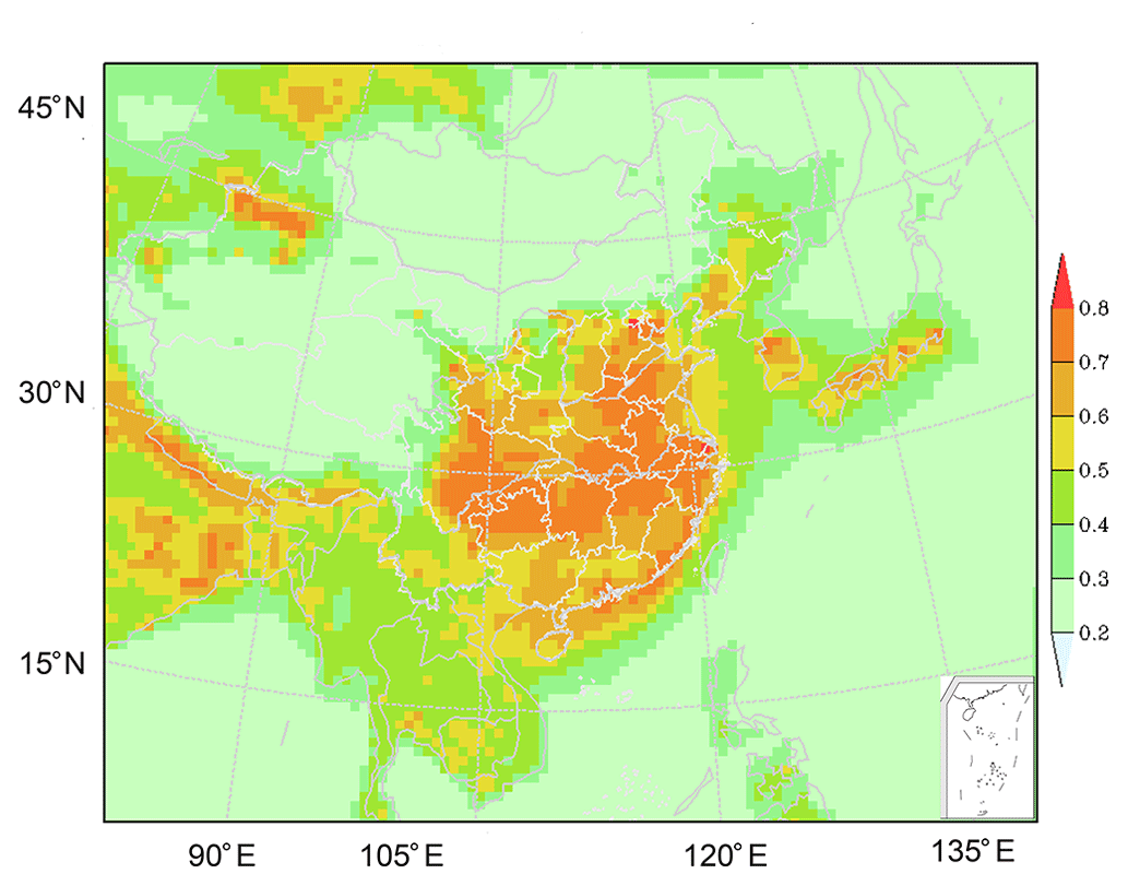
Figure 1 The ensemble spread of ${\mathit{\lambda }}_{i,t}^{\mathrm{a}}$ at model level 1 in January 2016, when β = 80.

The basic configuration of the JDAS CO₂ inversion settings followed previous studies. For instance, the ensemble size N was set to 50 to sustain the balance between computational cost and ensemble performance. The horizontal covariance localization radius was chosen as 1280 km to localize the observation's impact and ameliorate the spurious long-range correlations between state variables and observations caused by the limited number of ensemble members (Peng et al., 2023; Houtekamer and Mitchell, 2001; Gaspari and Cohn, 1999). Moreover, the covariance inflation factor β was set to 80 to preserve the ensemble spread. In this study, the assimilation window of EnKS was set to 24 h, and hour-by-hour assimilation was adopted in the novel flux forecast model and fine-scale CMAQ background simulation. In an assimilation cycle, the fluxes for the 24 h smoothing window were designed to be optimized hour by hour successively. The distribution of ensemble spread of CO₂ flux in January 2016 is provided in Fig. 1. It shows that the values of the ensemble spread range from 0.2 to 0.8 in most areas, which is consistent with our previous studies (Peng et al., 2015 in Fig. 11c and Peng et al., 2023).

2.3 GOSAT XCO₂ retrievals

GOSAT, launched by the Japan Aerospace Exploration Agency in January 2009, was designed to make near-global greenhouse gas measurements in a sun-synchronous orbit. It covers the whole globe in 3 d and has a sounding footprint of approximately 10.5 km. In this study, we assimilated GOSAT XCO₂ retrievals from NASA's Atmospheric CO₂ Observations from Space Level 2 standard data products (version ACOS_L2_Lite_FP.9r; data available at https://oco2.gesdisc.eosdis.nasa.gov/data/GOSAT_TANSO_Level2/, last access: 15 June 2023). This version of processing supports both nadir and glint soundings. In the case of soundings over water, a check was made to ensure the observation was made in glint mode. The XCO₂ data from Lite products were bias-corrected (Wunch et al. 2017; O'Dell et al. 2018). Typically, Level 2 Lite products contain 10–200 useful soundings per orbit, noting that more than 50 % of the spectral data were not processed during retrieval because they did not pass the first cloud screening preprocessing step.

The update for CO₂ flux is given by the observation innovation and the correlations between CO₂ concentrations and emissions, while the correlations are naturally provided by the physics- and dynamics-based numerical model. Although there are limited observation numbers, observations of 1 h are available. Thus through hourly updates, along with hourly model advances, the spatially sparse observations can sufficiently constrain the CO₂ flux, which can be demonstrated by the results. Given the EnKF algorithm, the posterior uncertainty is proportional to the prior uncertainty but with a smaller magnitude. Based on hourly update, the posterior uncertainty contains the same flow-dependent information as the prior uncertainty. For both chemistry assimilation and numerical weather prediction, it is common that the dimension of observation is much smaller than the dimension of state vector. Thus data assimilation helps to use the limited observations to constrain the state vector.

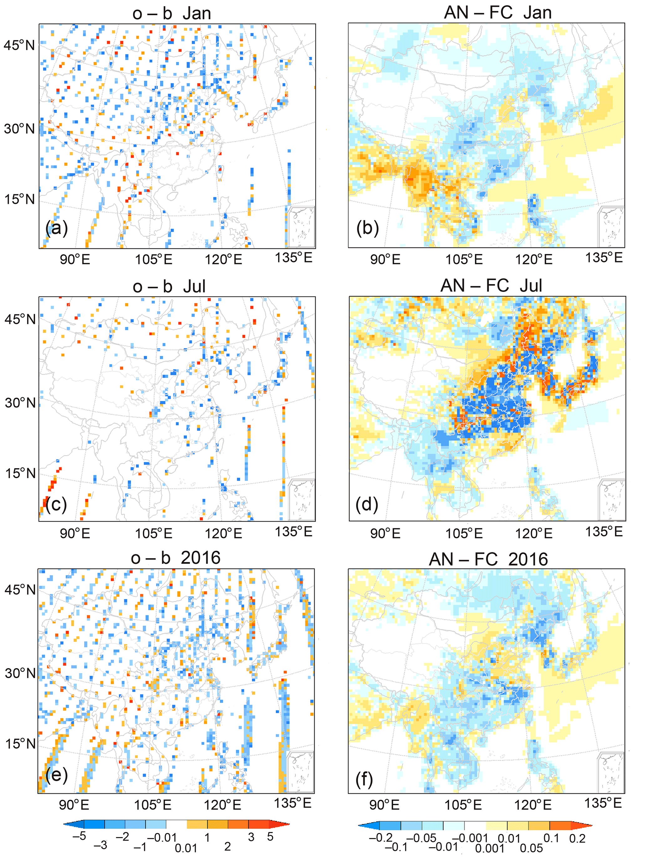
Figure 2 Observation increments (XCO₂; unit: ppm) and analysis increments (biosphere flux; unit: $\mathrm{\mu }\mathrm{mol}{\mathrm{m}}^{-\mathrm{2}}{\mathrm{s}}^{-\mathrm{1}}$) in (a, b) January, (c, d) July, and (e, f) the whole year of 2016.

Before being applied in assimilation, the GOSAT retrievals were operated in three steps. First, only the data retrievals tagged with “RetrievalResults/outcome_flag = 1” were selected, which indicates the retrieval quality. Second, to achieve the most extensive spatial coverage with the assurance of using the best-quality data available, a thinning strategy was used when multiple observations appeared in the same model grid point at the same hour on each day after interpolation of the model's horizontal coordinates. Only retrievals with a minimum value of uncertainty, i.e., “RetrievalResults/xco₂_uncert”, were selected. Third, the OMB quality control method is used to check the background fields to maintain stability in the assimilation. The records with absolute biases (i.e., |o−b|) greater than 5 ppm were removed, which are considered to have a lack of regional representativeness, and were mostly found near the boundary of the model domain. Moreover, the retrievals for the glint soundings over oceans have relatively larger uncertainty, and thus many data over oceans were excluded in our inversions in terms of the data-screening strategy (Fig. 2).

Non-assimilated XCO₂ observations were used for verification purposes after another process of repeated sifting, whose steps were as follows: (1) observations were marked with “outcome_flag = 1”; (2) XCO₂ values with the minimum “xco₂_uncert” in the same model grid point and at the same hour were excluded, which filtered out all of the assimilated XCO₂; and (3) outliers were precluded if the |o−b| was larger than 5.00 ppm.

2.4 Experimental design and evaluation method

Following previous GOSAT inversion work (Maksyutov et al., 2013; Feng et al., 2017; Wang et al., 2019; Liu et al., 2021; Jiang et al., 2022), in this study, the natural flux (i.e., biosphere–atmosphere exchange and ocean–atmosphere exchange) were optimized, while the fossil-fuel and biomass-burning fluxes were kept unchanged. This design, in which the natural fluxes were a subset of the state variables, further allowed us to focus on investigating the uncertainty of China's carbon sink, since the uncertainty in prescribed biomass-burning and fossil-fuel emissions is minor compared to that of the biosphere fluxes in the model domain (van der Werf et al., 2017; Zheng et al., 2018a; Kurokawa and Ohara, 2020). Fully reconciling the differences between bottom-up and inversion-estimated fossil-fuel emissions is outside the scope of this work and is therefore not discussed any further in this study. Consequently, the selected XCO₂ observations were assimilated hourly to adjust the CO₂ concentrations and fluxes. The assimilation was performed for the period 00:00 UTC 25 December 2015 to 23:00 UTC 31 December 2016, using the perturbed initial conditions and boundary conditions by adding Gaussian random noise with a standard deviation of 5 %. The first 7 d was set as the spin-up, which has been tested by Peng et al. (2015) with pseudo-satellite observation and CMAQ assimilation. Results for the period 1 January to 31 December 2016 are discussed and validated in detail in this paper.

Then, additionally, to assess the quality of the inversion results, two sets of forward simulations were performed throughout the year of 2016. One set of experiments was forced by the optimized a posteriori fluxes (denoted as FC), and the other was forced by the prescribed a priori fluxes as a control experiment (denoted as CTRL). Both forward runs used the same initial and boundary concentrations from the CT2019B product. Generally, it is hard to validate the optimized flux because comparison with in situ flux measurements is difficult on account of the discrepancy in scales between fluxes assimilated in the model grid point and eddy-covariance measurements over a very large uniform underlying surface. Therefore, this traditional approach was adopted as a compromise to assess whether the a posteriori fluxes would enable improvements in the fit to observed CO₂ concentrations, including non-assimilated GOSAT and surface observations from 14 sites.

Table 1 Evaluation results between the observations and model (unit: ppm), including model results from CTRL (black, a priori flux simulation), FC (italic, a posteriori flux simulation), and AN (bold, analysis fields from JDAS).

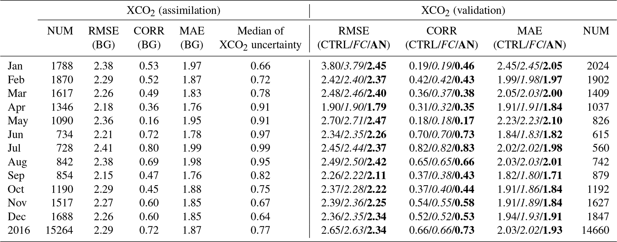
“XCO₂ (validation)” denotes the independent GOSAT XCO₂ retrievals for validation. “XCO₂ (assimilation)” represents the observations used for assimilation, and the corresponding model results come from BG (JDAS background fields). RMSE refers to the root-mean-square error, CORR refers to the correlation coefficient, MAE refers to the mean absolute bias, and NUM refers to the number of XCO₂ data. The monthly and annual averages were calculated from the hourly outputs.

3 Results

3.1 Performance of observational and analysis increments

We begin by analyzing the observational and analysis increment performance of JDAS. According to the statistics listed in Table 1, the total number of assimilated XCO₂ values in 2016 reached 15264 (i.e., 79.22 % of the thinned amount), with the monthly ratio of “assimilated-to-thinned” ranging from 74.19 % (in August) to 98.91 % (in July). The available XCO₂ data amount for JDAS decreases from 1788 in January to 1870 in February, to 734 in June, and to 728 in July, which represents an approximate 61 % reduction in the year-round monthly comparison. Also, it should be noted that the maximum median XCO₂ uncertainty occurred in July (0.99 ppm) and the minimum in December (0.64 ppm), indicating a better quality of XCO₂ retrievals in winter and less stable retrievals in summer. As shown in Table 1, both the mean absolute error (MAE) and root-mean-square error (RMSE) exhibit a maximum in July (1.99 and 2.41 ppm, respectively) and a minimum in April and September (MAE: 1.76 and 1.76 ppm; RMSE: 2.18 and 2.15 ppm), indicating that the point-by-point uncertainty is larger in summer and lower in spring and autumn, which is consistent with previous model studies (Li et al., 2017). The difference in seasonal performance could be partly due to the uncertainties in the spatial and temporal variations of the biosphere flux estimation and fossil-fuel inventories.

Figure 2 demonstrates the distribution of XCO₂ observation increments and CO₂ flux analysis increments (i.e., the analysis-minus-background E^a−E^b) over the model domain, including January (Fig. 2a and b), July (Fig. 2c and d) and the whole year (Fig. 2e and f). In particular, most of the available XCO₂ in July appears in the north and central region of China, but the south and northwest tend to be blank. The XCO₂ innovation range is usually between −3 and 3 ppm in the corresponding model grid point, with a monthly mean value between −0.12 and −0.96 ppm over the model domain. Moreover, the pattern of CO₂ flux analysis increments (i.e., AN–FC flux) preserves features from innovations and certifies that GOSAT XCO₂ is effectively absorbed in JDAS. GOSAT retrievals were found to display impacts within a certain range near the observation points after entering the assimilation system. The higher variation in monthly flux analysis increments for July than those for January indicates that the uncertainties of forecast flux in summer are larger than those of the variation in winter. Considering the peculiarities of atmospheric CO₂, such as its long atmospheric lifetime, long-range transport, high background concentrations, and strong biosphere–atmosphere exchanges, there are both wide-ranging overall increases (e.g., −0.01 to 0.1 over central China) and decreases (e.g., −0.2 to −0.01 over South China) and small-scale adjustment taking place in 2016 (Fig. 2f).

Table 2 China's annual carbon sink estimated by different methods, including the inventory method, ecosystem process models, and atmospheric inversion (unit: Pg C yr⁻¹).

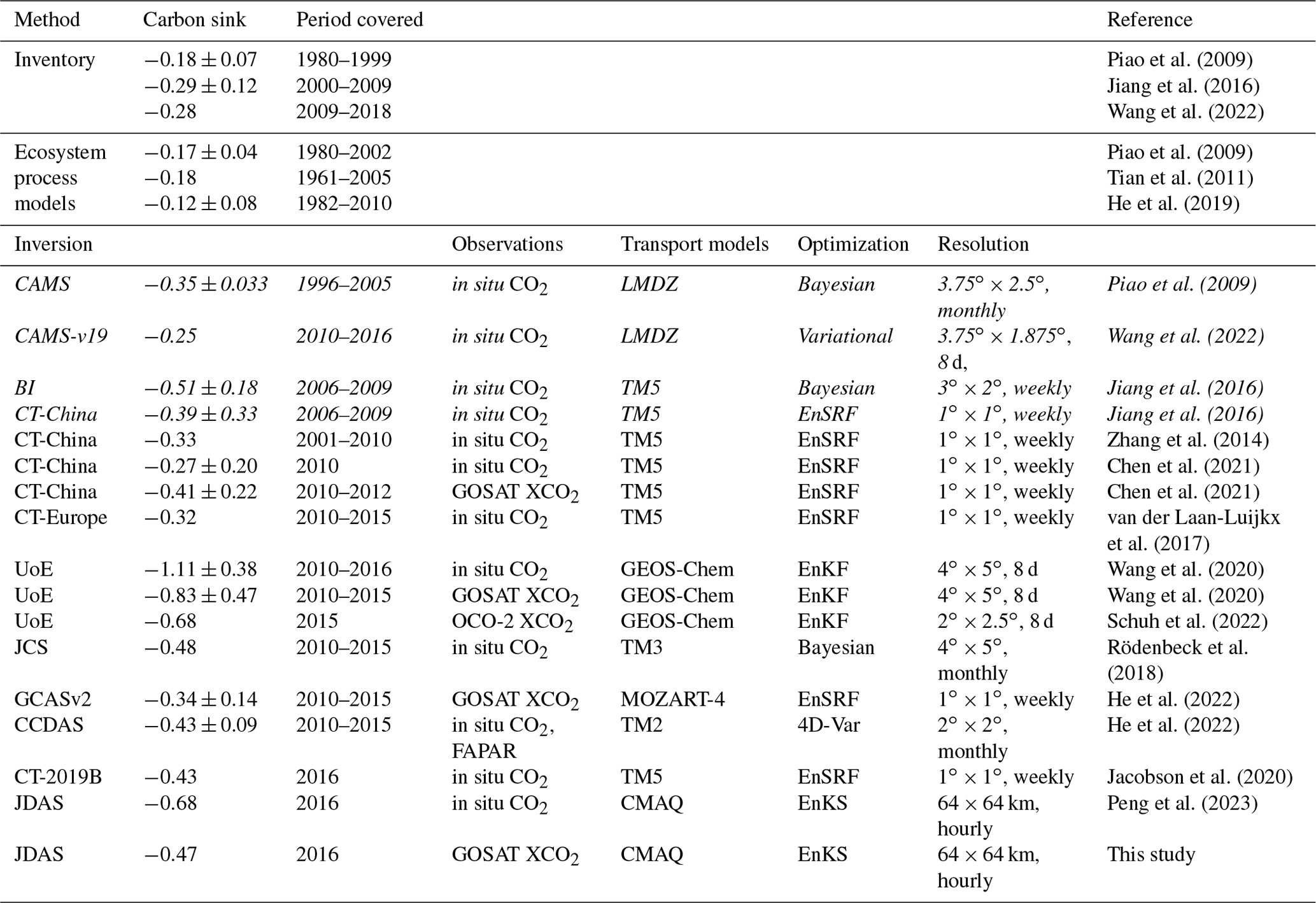
Italic font denotes the inversion results after correcting for lateral fluxes according to the flux gap between top-down and bottom-up estimation. The abbreviations used in the table are as follows: CAMS, Copernicus Atmosphere Monitoring Service; BI, Bayesian inversion; JCS, Jena CarboScope; CCDAS, Carbon Cycle Data Assimilation System; FAPAR, remotely sensed Fraction of Absorbed Photosynthetically Active Radiation; LMDZ, Laboratoire de Météorologie Dynamique Zoom, a global transport model; and TM5, the global atmospheric Tracer Model 5.

3.2 Size of the annual carbon sink in China

Before presenting a posteriori biosphere fluxes in China from JDAS, Table 2 provides an overview of most of the well-known inversion modeling systems, configurations of inversions, atmospheric transport models, spatiotemporal resolutions, and observations. The inversion systems differ by the transport model, the inversion approach, the choice of observation, and prior constraints, enabling us to facilitate international comparison and mutual recognition. For example, either in situ CO₂ or GOSAT XCO₂-constrained flux (i.e., −1.11 and −0.83 Pg C yr⁻¹) demonstrates much higher sink estimates from GEOS-Chem-based inversion with a 4^∘ × 5^∘ horizontal resolution. Excluding the outliers, most global inversions report a carbon sink in China of −0.27 to −0.56 Pg C yr⁻¹ from in situ CO₂ and −0.34 to −0.68 Pg C yr⁻¹ from satellite retrievals. In contrast, our estimates constrained by GOSAT observation (−0.47 Pg C yr⁻¹) agree reasonably well with the previous estimates mentioned above.

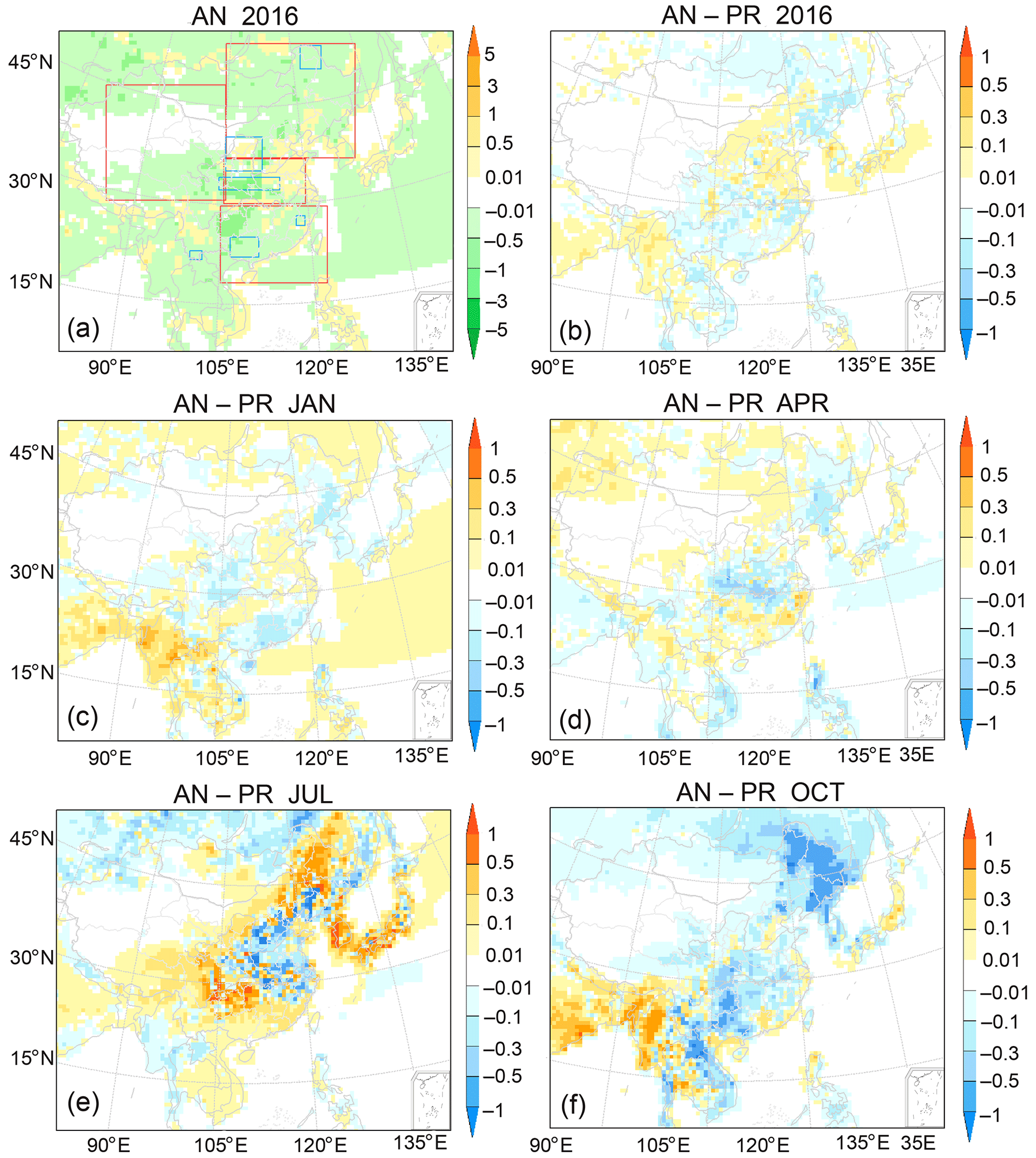
Figure 3 Horizontal distribution of CO₂ biosphere fluxes (unit: $\mathrm{\mu }\mathrm{mol}{\mathrm{m}}^{-\mathrm{2}}{\mathrm{s}}^{-\mathrm{1}}$): (a) E^a in 2016, the a posteriori fluxes; (b) E^aE^p in 2016, the differences between the a posteriori and a priori CO₂ fluxes; (c) E^aE^p in January; (d) E^aE^p in April; (e) E^aE^p in July; (f) E^aE^p in October. The red frames mark west China (28–48^∘ N, 85–104^∘ E), north China (37–52^∘ N, 105–135^∘ E), central China (30–36^∘ N, 105–120^∘ E), and south China (18–29^∘ N, 105–123^∘ E). The blue frames mark six key ecological areas of China: Daxing'anling (50–53^∘ N, 121–127^∘ E), the Loess Plateau (35–40^∘ N, 105–112^∘ E), the Qinling Mountains (32–34^∘ N, 104–115^∘ E), the rocky desert in Guangxi (22–25^∘ N, 106–111^∘ E), Mount Wuyi (26.5–28.0^∘ N, 117.5–119.0^∘ E), and Xishuangbanna (21.0–22.6^∘ N, 100.0–102.0^∘ E).

3.3 Regional characteristics of posterior fluxes

As can be seen in Fig. 3a, the annual horizontal distribution patterns of biosphere flux show significant spatial heterogeneity and fairly large gradients in most areas. Fig. 3b further illustrates annual differences between a priori and a posteriori fluxes over the model domain. Although China's total carbon sink of a posteriori fluxes (−0.47 Pg C yr⁻¹) is approximately equal to the a priori fluxes (−0.43 Pg C yr⁻¹), the spatial distribution has been modified through assimilation. Compared to the prescribed a priori biosphere flux, not only large-scale vegetation adjustments but also small-scale conditions can be detected throughout the year after assimilating atmospheric observations (Fig. 3b). Generally, the a priori biosphere fluxes are overestimated (∼ 0.1–0.3 $\mathrm{\mu }\mathrm{mol}{\mathrm{m}}^{-\mathrm{2}}{\mathrm{s}}^{-\mathrm{1}}$) in the north (dominated by forest, grassland and cropland) and south (dominated by forest and grassland) of China, while they are underestimated (∼ 0.1–0.5 $\mathrm{\mu }\mathrm{mol}{\mathrm{m}}^{-\mathrm{2}}{\mathrm{s}}^{-\mathrm{1}}$) primarily in central China where there is a large area of cropland.

Figure 3c–f show the seasonal spatial differences before and after assimilation, taking January, April, July, and October as representatives of winter, spring, summer, and autumn. The monthly averages were calculated from the daily averages based on hourly outputs. The difference between the analysis and prior flux tends to be larger in July, lower in April and October, and lowest in January, which indicates a larger uncertainty in biosphere flux estimates in the growing season. This is consistent with the findings of previous studies (Jiang et al., 2016; Chen et al., 2021; Fu et al., 2022). Moreover, it should be noted that an obvious underestimation of a priori flux (approximately 0.1–0.5 $\mathrm{\mu }\mathrm{mol}{\mathrm{m}}^{-\mathrm{2}}{\mathrm{s}}^{-\mathrm{1}}$) occurs in the northern, central, and southern vegetation growth regions. On the other hand, the central part of China, dominated by cropland, shows relatively larger a posteriori flux in winter and smaller a posteriori flux in summer and autumn, in contrast with the a priori flux constrained by the limited background observation sites (Zhang et al., 2014; Jacobson et al., 2020). Additionally, compared with the weekly temporal resolution of global inversion, the hourly observational increments as well as the hourly first-guess fields in this study hold some advantage in evaluating the monthly variations of fluxes. As expected, some distinguishing features are thus demonstrated in the assimilated fluxes, such as the carbon sources in parts of central, eastern, and southwest China, which is more consistent with the underlying surface situation. In this way, the JDAS inversion system has the potential to depict the fine-scale characteristics of biosphere flux.

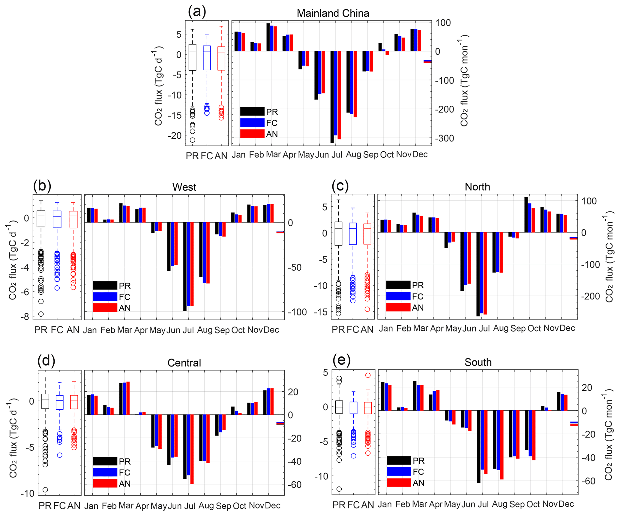
Figure 4 Time series of CO₂ biosphere fluxes over (a) mainland China, (b) west China, (c) north China, (d) central China, and (e) south China, marked by the red frames in Fig. 3a (unit: Tg C per month), in each month of 2016, obtained from a priori values (PR, black), a posteriori values (AN, red), and the flux forecast model (FC, blue). The bars on the right-hand side represent the 12-month average (unit: Tg C per month). The boxes on the left-hand side denote the daily flux (unit: Tg C d⁻¹), with the whiskers indicating the minimum and maximum and the horizontal lines across the box indicating the 25th percentile, the median, and the 75th percentile, respectively.

Next, we analyze the monthly and annual fluxes in five large regions – west, north, central, south, and mainland China (denoted by the red frame in Fig. 3a) – to analyze the regional inversion in subcontinental-scale flux variation as well as to contrast results with the previous inversion analysis (Fig. 4). Given the representative background and observation information, the seasonality patterns were modified by JDAS assimilation, with larger annual sinks relative to the a priori ones and a growing season that is shifted earlier in the year over central and south China. As shown in Fig. 4, there is an evident difference in the a posteriori annual carbon sink magnitude in these regions, gradually decreasing in the north (e.g., forest, grassland and cropland), south (e.g., forest and grassland), west (e.g., grassland and tundra), and central region (e.g., cropland) in turn, which is consistent with the primary corresponding ecosystem types, while the a priori sink of the west tends to be larger than that of the south. Using the north as a reference, the annual carbon sinks of the a priori estimates for the north, south, west, and central regions are 1.00, 0.57, 0.62, and 0.44, respectively, while those of the a posteriori estimates are 1.00, 0.62, 0.56 and 0.38. On the other hand, the a priori and a posteriori amplitudes of the seasonal variation (i.e., the difference between the maximum and minimum monthly estimates, as defined in Crowell et al., 2019) range from 374.33/333.74, 87.01/80.41, 120.33/113.98, and 82.34/88.00 to 413.17/389.48 Tg C per month in north, south, west, central, and mainland China, respectively. Moreover, the drastic fluctuation in the daily variation of prior fluxes has been modified by observational constraints in JDAS (sub-graph in the left-hand panel of Fig. 4). Therefore, this implies the potential for regional inversion in interpreting underlying processes in large regions such as China where the ecosystems and climate are quite varied.

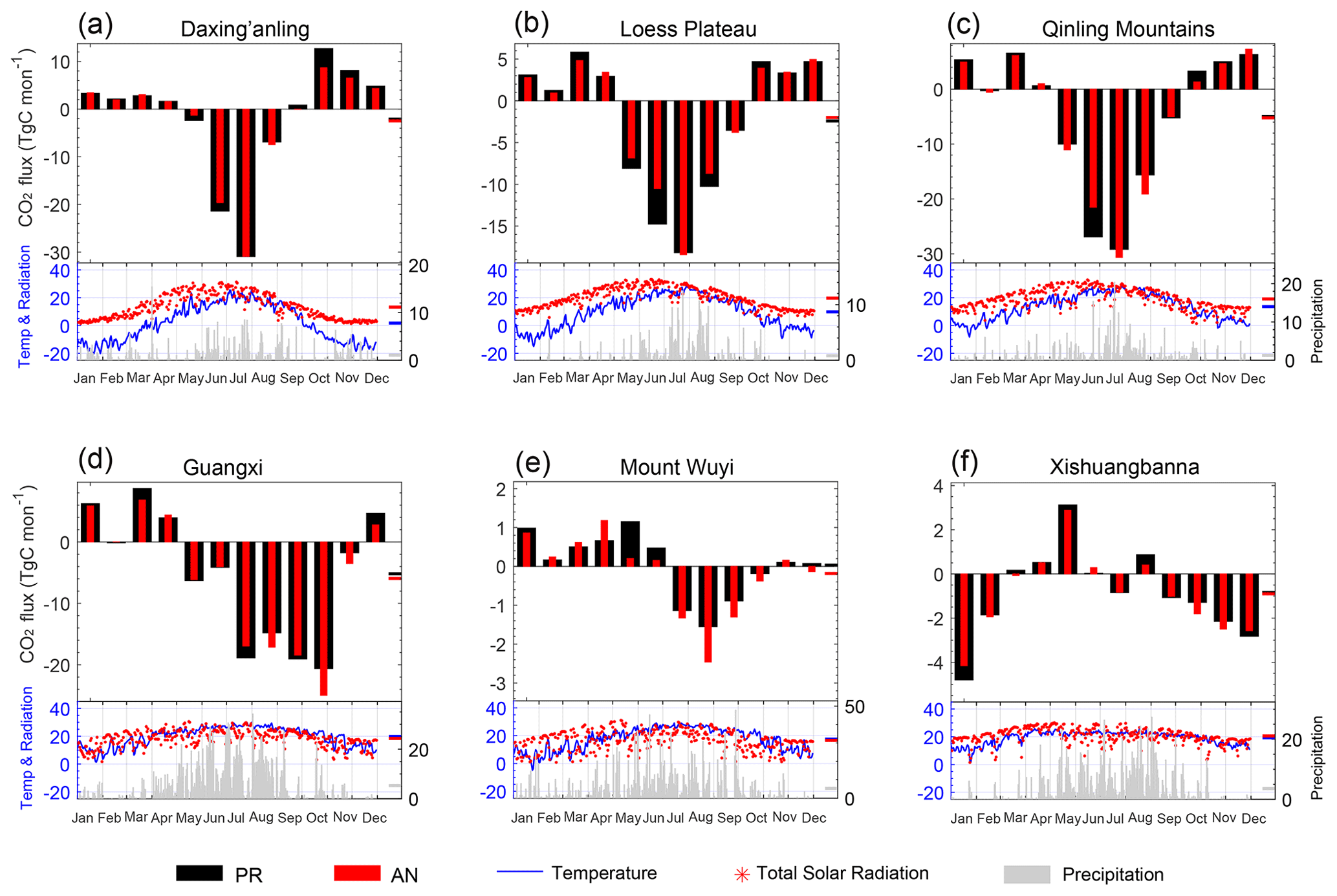
Figure 5 Time series of CO₂ biosphere fluxes over six ecological areas of China (blue frames in Fig. 3a; unit: Tg C per month), in each month of 2016, obtained from a priori values (PR, black bars) and a posteriori values (AN, red bars). The bars on the right-hand side represent the 12-month average (unit: Tg C per month). The subfigures at the bottom denote the daily temperature (blue lines; unit: ^∘; left-hand y axis), total solar radiation (red stars; unit: MJ d⁻¹; left-hand y axis), and precipitation (grey bars; unit: mm d⁻¹; right-hand y axis), with the right-hand bars representing the annual average.

Nevertheless, achieving robust and reliable flux signals at smaller regional scales is quite demanding and rather challenging because of the limited observations and low accuracy of transport models as well as the a priori information. In this paper, we further try to investigate the condition of the regional biosphere carbon sink over several of China's key ecological areas (denoted by the blue frame in Fig. 3a) – for example, Daxing'anling (DX), the Loess Plateau (HT), the Qinling Mountains (QL), the rocky desert in Guangxi (SM), Mount Wuyi (WY), and Xishuangbanna (XS). These regions are characterized by their unique vegetation and climatic conditions. In particular, the a priori and a posteriori seasonal amplitudes amount to 43.64/39.56, 24.03/23.39, 35.73/37.96, 29.36/31.80, 2.70/3.64, and 7.93/7.04 Tg C per month in DX, HT, QL, SM, WY, and XS, respectively. The DX region is characterized by abundant forest and far more satellite retrievals to constrain fluxes, with annual a priori and a posteriori carbon sinks of −25.13/−29.64 Tg C yr⁻¹. Compared to a priori fluxes, relatively stronger a posteriori sinks are also found in QL (−60.05/−62.53 Tg C yr⁻¹), SM (−62.10/−71.27 Tg C yr⁻¹), WY (0.36/−2.19 Tg C yr⁻¹), and XS (−10.12/−10.79 Tg C yr⁻¹), which is consistent with the improved ecological conditions due to ecological engineering construction as well as generally favorable climatic conditions. As can be seen in Fig. 5, the XS region is unique and worthy of attention in contrast to the other regions not only because it shows different seasonality in its release of CO₂ to the atmosphere in summer and removal of CO₂ from the atmosphere in other seasons but also because of the large transport model errors that are included in the model–data mismatch error involved in previous inversion studies (J. Wang et al., 2020; He et al., 2022; Schuh et al., 2022; Wang et al., 2022; Y. L. Wang et al., 2020). Thus, the abovementioned spatial variations of a posteriori fluxes might unlock some of the potential local signals in areas where regional transport models are more reliable and observations are plentiful.

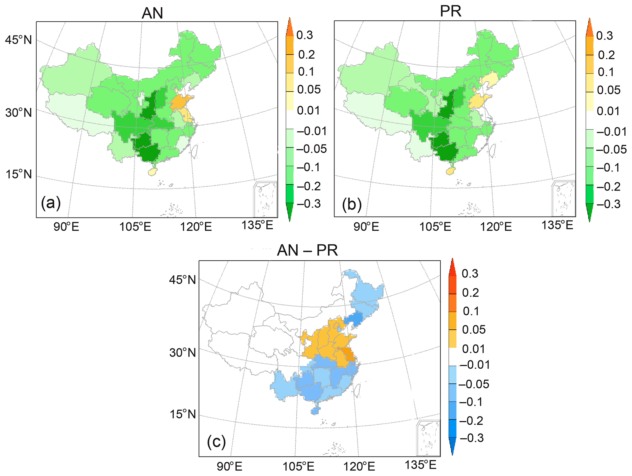
Figure 6 Horizontal distribution of CO₂ biosphere fluxes averaged over each province of mainland China in 2016 (unit: $\mathrm{\mu }\mathrm{mol}{\mathrm{m}}^{-\mathrm{2}}{\mathrm{s}}^{-\mathrm{1}}$): (a) E^a, the a posteriori fluxes; (b) E^p, the a priori fluxes; and (c) E^aE^p, the differences between the a posteriori and a priori CO₂ fluxes. Note that Taiwan, Hong Kong SAR, Macao SAR, and Shanghai are not discussed owing to the insufficient grid resolution.

3.4 Provincial patterns of optimized fluxes

In this section, we investigate the provincial patterns of biosphere flux (Fig. 6). Based on the gridded a posterior flux dataset, we first assess the annual CO₂ biosphere sink levels in 31 provinces in mainland China (Taiwan, Hong Kong SAR, Macao SAR, and Shanghai are not discussed because of the insufficient grid resolution). At this scale, both the a priori and a posteriori fluxes indicate the strongest carbon sink intensity per unit area being in Shaanxi, Guangxi, and Guizhou, but the a priori fluxes produce an underestimation in Shanxi and overestimations in Guangxi and Guizhou, respectively. Next, the second strongest carbon sink intensity is commonly seen in Shaanxi, Sichuan, Chongqing, and Hubei, whereas a comparatively low level of carbon sink intensity appears in Xinjiang, Liaoning, Anhui, and Yunnan as well as in Tibet and Fujian. Furthermore, some provinces with neutral (i.e., close to 0) source or sink statuses are re-evaluated by the GOSAT-constrained fluxes (Fig. 6a and b). For instance, the a posteriori flux in Ningxia is −0.01–0.01 $\mathrm{\mu }\mathrm{mol}{\mathrm{m}}^{-\mathrm{2}}{\mathrm{s}}^{-\mathrm{1}}$, while the a priori flux displays a weak carbon sink of −0.01 to −0.05 $\mathrm{\mu }\mathrm{mol}{\mathrm{m}}^{-\mathrm{2}}{\mathrm{s}}^{-\mathrm{1}}$, due to the complexity in the estimation related to the grassland and cropland land surfaces in this province. On the contrary, the a priori fluxes in Fujian and Jiangsu are close to 0, but we find a carbon sink ranging from approximately −0.01 to −0.05 $\mathrm{\mu }\mathrm{mol}{\mathrm{m}}^{-\mathrm{2}}{\mathrm{s}}^{-\mathrm{1}}$ and a carbon source from 0.05 to 0.1 $\mathrm{\mu }\mathrm{mol}{\mathrm{m}}^{-\mathrm{2}}{\mathrm{s}}^{-\mathrm{1}}$, respectively. For Liaoning, the a priori fluxes are characterized by CO₂ sources (0.01–0.05 $\mathrm{\mu }\mathrm{mol}{\mathrm{m}}^{-\mathrm{2}}{\mathrm{s}}^{-\mathrm{1}}$), while the assimilated fluxes with satellite measurements are slightly adjusted to a carbon sink (−0.05–0.1 $\mathrm{\mu }\mathrm{mol}{\mathrm{m}}^{-\mathrm{2}}{\mathrm{s}}^{-\mathrm{1}}$).

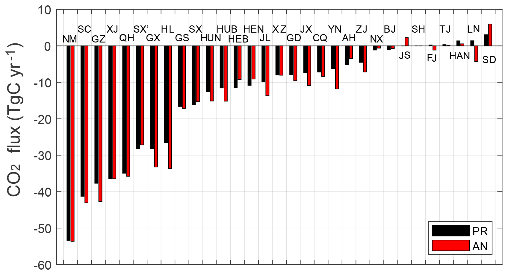
Figure 7 The total a priori (black) and a posteriori (red) CO₂ biosphere fluxes over each province of mainland China in 2016 (unit: Tg C yr⁻¹). The abbreviations of the provinces are NM, Neimenggu; SC, Sichuan; GZ, Guizhou; XJ, Xinjiang; QH, Qinghai; SX', Shaanxi; GX, Guangxi; HL, Heilongjiang; GS, Gansu; SX, Shanxi; HUN, Hunan; HUB, Hubei; HEB, Hebei; NEN, Henan; JL, Jilin; XZ, Xizang; GD, Guangdong; JX, Jiangxi; CQ, Chongqing; YN, Yunnan; AH, Anhui; ZJ, Zhejiang; NX, Ningxia; BJ, Beijing; JS, Jiangsu; SH, Shanghai; FJ, Fujian; TJ, Tianjin; HAN, Hainan; LN, Liaoning; and SD, Shandong.

Lastly, the sizes of the provincial biosphere fluxes are summarized and sorted quantitatively in Fig. 7. The maximum and minimum provincial biosphere flux sizes are in Inner Mongolia (a posteriori: −53.65 Tg C yr⁻¹; a priori: −53.41 Tg C yr⁻¹) and Shandong (a posteriori: 5.99 Tg C yr⁻¹; a priori: 3.05 Tg C yr⁻¹), respectively. Moreover, the difference between the a posteriori and a priori provincial flux ranges from −7.03 Tg C yr⁻¹ in Heilongjiang to 2.95 Tg C yr⁻¹ in Shandong, with an underestimation greater than 2.00 Tg C yr⁻¹ appearing in Shandong (2.95), Jiangsu (2.31), and Hebei (2.25) and an overestimation greater than 5.00 Tg C yr⁻¹ appearing in Heilongjiang (7.03), Liaoning (5.68), Yunnan (5.59) and Guangxi (5.10). On the other hand, a smaller percentage of modification between the a posteriori and a priori flux (i.e., (a posteriori − a priori)$/$a priori × 100 % in absolute value) arises in Xinjiang (0.28 %), Inner Mongolia (0.46 %), Tibet (1.10 %), Qinghai (2.45 %), Gansu (3.21 %), Shaanxi (3.50 %), Sichuan (4.34 %) and Shanxi (4.65 %), indicating a lower level of uncertainty in these larger carbon-sink provinces. Nevertheless, an increased percentage of modification in provincial flux appears in Jiangsu (a posteriori: 2.29 Tg C yr⁻¹; a priori: −0.02 Tg C yr⁻¹), Liaoning (a posteriori: −4.27 Tg C yr⁻¹; a priori: 1.40 Tg C yr⁻¹), Fujian (a posteriori: −1.15 Tg C yr⁻¹; a priori: 0.29 Tg C yr⁻¹), and Shandong (already listed above).

3.5 Evaluation against observations

We further assess the performance of the a posteriori CO₂ fluxes by comparing the CTRL, FC, and AN results in the fit to non-assimilated GOSAT as well as surface observations. The monthly and annual statistics were computed from the hourly outputs from the assimilation, simulation and observations. Table 1 demonstrates (as expected) that the concentration from the analysis fields (AN) performs best when fitted to the non-assimilated XCO₂ observations. It is notable that the column-averaged satellite signals have limited capacity in facilitating the tropospheric variation in CO₂ concentration compared to surface observations. Thus the response to changes in the simulated XCO₂ signal is weak, and improvement is rather moderate. For instance, the annual RMSE, MAE, and correlation coefficient for AN are 2.34 ppm, 1.93 ppm, and 0.73; for FC, they are 2.63 ppm, 2.02 ppm, and 0.66; and for CTRL, they are 2.65 ppm, 2.03 ppm, and 0.66, respectively. Additionally, the AN, FC, and CTRL biases from non-assimilated XCO₂ observations are further calculated (Table 3), and the outliers in CTRL have been effectively amended. When FC is compared with the CTRL results, the frequency of bias in [−4, 4] increases by 0.25 %, in [−3, 3] by 0.36 %, in [−2, 2] by 0.32 %, and in [−1, 1] by 0.14 %. The error standard deviation decreases from 2.63 ppm in CTRL to 2.61 ppm in FC and to 2.27 ppm in AN.

Table 3 Probability distribution of hourly bias (unit: %) and bias standard deviation (unit: ppm) of XCO₂ validation including CTRL, FC and AN in 2016.

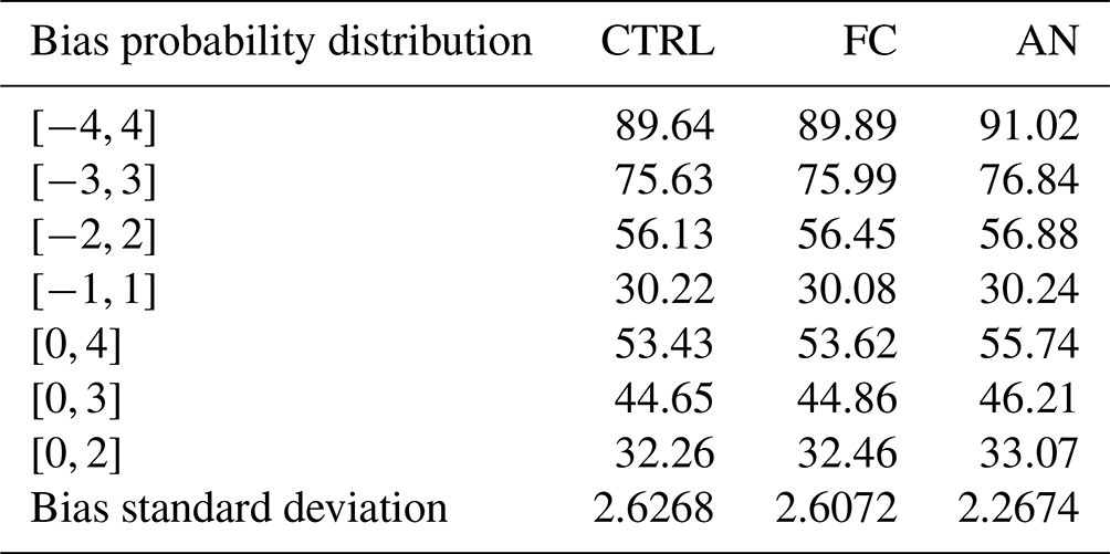
Table 4 Evaluation results between in situ observations and model, including CTRL (black, a priori flux simulation), FC (italic, a posteriori flux simulation), and AN (bold, analysis fields from JDAS).

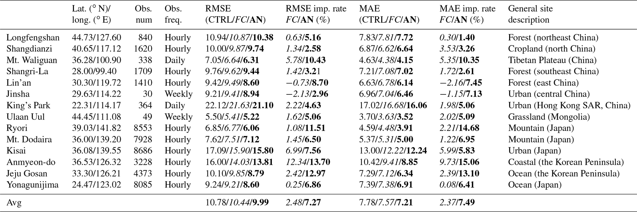
“Lat./long.” refers to the latitude and longitude of the site; “Obs. num” refers to the observation amount; “Obs. freq.” refers to the observation time frequency; “RMSE imp. rate” refers to the improvement rate of RMSE, i.e., $({\mathrm{RMSE}}_{\mathrm{CTRL}}-{\mathrm{RMSE}}_{\mathrm{FC}})/{\mathrm{RMSE}}_{\mathrm{CTRL}}$ × 100 % and $({\mathrm{RMSE}}_{\mathrm{CTRL}}-{\mathrm{RMSE}}_{\mathrm{AN}})/{\mathrm{RMSE}}_{\mathrm{CTRL}}$ × 100 %; “MAE imp. rate” refers to the improvement rate of MAE, i.e., $({\mathrm{MAE}}_{\mathrm{CTRL}}-{\mathrm{MAE}}_{\mathrm{FC}})/{\mathrm{MAE}}_{\mathrm{CTRL}}$ × 100 % and $({\mathrm{MAE}}_{\mathrm{CTRL}}-{\mathrm{MAE}}_{\mathrm{AN}})/{\mathrm{MAE}}_{\mathrm{CTRL}}$ × 100 %, respectively. The annual averages were calculated from the hourly output.

Furthermore, surface in situ observations from 14 sites are further used as independent observations to evaluate the inversion results. The modeled CO₂ concentrations were extracted from the simulated hourly CO₂ fields according to the locations, elevation, and time of each observation. The averages of observation, CTRL, FC, and AN over these 14 stations are 410.97, 413.01, 412.82, and 412.21 ppm, respectively. The statistics of the analytical field (AN) in Table 4 are better than FC and CTRL, including RMSE and MAE, which gives a direct indication that the assimilation performs well. Taking improvement rate as example, the RMSE improvement rate between the FC and CTRL mostly ranges from −2.13 % to 12.34 % with an average of 2.48 %, and the MAE improvement rate ranges from 0.08 % to 9.73 % with an average of 2.37 %. Although the RMSE and MAE of AN are lower than CTRL and FC, those of FC are higher than CTRL in Lin'an (in Wuhan, Hubei) and Jinsha (in Yangtze River Delta), which are in the vicinity of urban clusters with increased human activity (Liang et al., 2023). Thus, this helps to check that the inversions actually improve the model fits to the observations but also to determine whether some sites are particularly problematic for natural flux inversions. Inversions actually improve the model fits to the surface observations in forest areas (in northeast, east, and southeast China), cropland areas (in north China), grassland areas (in Mongolia), ocean (in the Korean Peninsula and Japan), and coastal areas (in the Korean Peninsula).

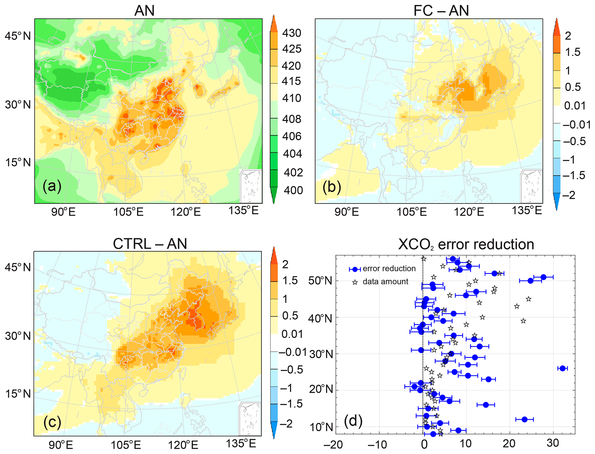
Figure 8 The annual-averaged horizontal distribution of CO₂ concentrations (unit: ppm) near the surface in 2016: (a) AN, the analysis concentration; (b) FC − AN, the difference between the a posteriori flux simulation and analysis concentration fields; (c) CTRL − AN, the difference between the a priori flux simulation and analysis concentration fields; and (d) the XCO₂ error reduction (see text for calculation; blue, with the standard deviation (±) of the analysis XCO₂ provided) and independent XCO₂ data amount (black stars, rescaled to 1:10) over 8–57^∘ N and 105–120^∘ E at different latitudes.

The annual-averaged horizontal distributions of CO₂ concentration near the surface in 2016 are presented (Fig. 8). Figure 8a displays the surface CO₂ concentration analysis fields (AN), and the much-refined description in the AN allows for a more detailed characterization of the spatiotemporal distribution of CO₂ concentration and can further facilitate an interpretation of satellite data in a regional context over China. Thus, the AN can be used as a closer representation of the real condition. As shown in Fig. 8b and c, compared to the CTRL fields, the FC fields tend to be considerably closer to the AN fields, suggesting that a posteriori fluxes are calibrated acceptably. Furthermore, Fig. 8d shows the year-round statistic of XCO₂ error reduction (defined as ($\mathrm{1}-{\mathit{\delta }}_{\text{FC}}/{\mathit{\delta }}_{\text{CTRL}})\times \mathrm{100}\mathit{\%}$)), as well as the amounts of non-assimilated XCO₂ observations, where δ_FC represents the FC XCO₂ error standard deviation and δ_CTRL the CTRL XCO₂ error standard deviation. The region of 8–57^∘ N and 105^∘−120^∘ E is used as a reference because there is a relatively larger difference between the a priori and a posteriori fields, including the concentration as well as flux. In general, the error reduction is primarily found to be positive and ranges from approximately 0.80 % to 32.13 % with a median of 5.65 % and mean of 7.23 %. This zonal evaluation further verifies the improvement in the a posteriori flux compared to the a priori flux.

4 Discussion

4.1 China's carbon sink international comparability among different methods

The total annual carbon sink in previous research along with our study is summarized (Table 2). The aim is mainly to check that different methods – for instance, inventories, ecosystem process models, and atmospheric inversions – actually improve the carbon sink international comparability and mutual recognition. Based on national ecosystem inventory data, China's terrestrial carbon sink increased from −0.18 Pg C yr⁻¹ in the 1980s to −0.33 Pg C yr⁻¹ in the 2000s owing to forest area expansion and afforestation during recent years (Piao et al., 2009; Jiang et al., 2016; Wang et al., 2022). Meanwhile, the results from several ecosystem process-based models display a carbon sink ranging from −0.13 to −0.22 Pg C yr⁻¹ during 1980–2010, achieved by assessing the effect of changes in climate and CO₂ (Piao et al., 2009; He et al., 2019). In addition, according to the flux gap between top-down and bottom-up estimations mentioned above, a recent estimate of the lateral flux for China is −0.14 Pg C yr⁻¹, which includes the carbon exchange between the land and atmosphere in non-CO₂ forms as well as imported wood and crop products (Wang et al., 2022).

The terrestrial carbon sink in 2016 with lateral fluxes adjustment amounts to approximately −0.33 Pg C yr⁻¹, constrained by the GOSAT XCO₂ in JDAS (−0.47 Pg C yr⁻¹). Correspondingly, we also provide a corrected carbon sink estimate of −0.54 Pg C yr⁻¹ (i.e., −0.68 + 0.14 = −0.54) inferred from in situ CO₂ data provided by JDAS (Peng et al., 2023), which is the optimal mathematical solution under the current sparse observational coverage with daytime photosynthetic uptake and likely leads to a slight overestimation to some extent. Hence, our estimates (−0.68 and −0.47 Pg C yr⁻¹ from in situ CO₂ and GOSAT, respectively) agree reasonably well with the previous estimates mentioned above.

4.2 To what extent is the JDAS's posterior flux different from the prior flux?

In general, most research into the inversion of China's carbon sink has commonly used global transport models. The limited resolution and distribution of observations are deemed to lead to large uncertainties in inversion in small regions, especially at national scales (Crowell et al., 2019; Monteil et al., 2020; Piao et al., 2022). The resolution-related performance of transport models tends to magnify the uncertainty in China's carbon sink estimates. For instance, Fu et al. (2021) found that the results of a global model (i.e., GEOS-Chem) tended to be generally lower than GOSAT's XCO₂ in China from the various terrestrial models with a mean bias of about 2 ppm in winter, while Lei et al. (2014) found GEOS-Chem simulations tended to produce higher values than GOSAT (by 5.8 ppm) in China during summer. In contrast, the observational increments of JDAS show an ability to depict the fine-scale features with strong spatial heterogeneity whilst in general retaining the large-scale spatial patterns, which can be attributed to the CMAQ simulation performance in differentiating the nuances of anthropogenic and natural conditions. On the other hand, the analysis increments depend not only on the innovations, but also on how well the Kalman gain matrix computes the contribution weighting factors based on the time-dependent forecast error covariance. The biosphere flux first-guess fields were derived from the novel flux forecast model by taking the a priori flux, the analysis flux from the previous assimilation cycle, and the forecast concentration (Eq. 1), which is a great help in assisting with improving the background information and initial perturbation for ensemble forecasting.

The good response of the vegetation condition to the a posteriori results provides a strong foundation for a meaningful interpretation of biosphere fluxes. Satellites, with their better spatial coverage, as well as regional transport models, with their improved stability, can help in assessing the real conditions of local terrestrial ecosystems with complex conditions, such as over central China. The decreased annual sink and increased seasonal variability in central China deduced by the a posteriori flux with satellites may in fact reflect the atmospheric CO₂ fixed by cropland vegetation, where ∼ 60 % of the area is cropland with relative few in situ observations used for constraining the a priori flux (Piao et al., 2009, 2022). Actually, downward correction over forest and grassland and upward correction for cropland areas have been validated against independent data. Inversions actually improve the model fits to the surface observations in cropland, forest, and grassland areas. In general, (1) widespread underestimation of the a priori flux (0.01–0.1 $\mathrm{\mu }\mathrm{mol}{\mathrm{m}}^{-\mathrm{2}}{\mathrm{s}}^{-\mathrm{1}}$) is found in central China, which is dominated by cropland and where dense satellite retrievals are accordingly available; (2) overestimates are distributed in the northeast and south of China over a considerable spatial extent; and (3) smaller changes between a posteriori and a priori estimates are primarily located in the west of China, which tends to agree with the XCO₂ OMB pattern. Nevertheless, summer is the season with the largest percentage of satellite data rejection and retrieval uncertainty, still making it a tough test for inversion systems.

At the provincial scale, the provinces in China differ in both terrestrial vegetation and anthropogenic activity. As discussed earlier, the difference between a posteriori and a priori estimates is closely related to the degree of human activity intervention. Several factors could account for the provincial spatial distribution constrained by GOSAT, for instance, the increased precipitation along with the strong El Niño in 2016, the levels of reforestation and afforestation, and the reductions in biofuels in rural areas bringing about a shrubland carbon sink.

4.3 How well can the JDAS inversion constrain the carbon sink of China?

Quantitative information on the extent of which the posterior fluxes are constrained by observations has been checked further. The prior information has been embodied in a priori-flux-simulated concentrations, and observation information has been embodied in the a posteriori flux simulation, whose fluxes are constrained by observations. By evaluating the differences between these two sets of simulation results, the prior information and observation information are now accessible in order to be assessed quantitatively. At the site scale (Table 4), some sites tend to systematically be poorly fitted by the inversions, in particular those in the vicinity of large urban areas with large anthropogenic emissions, such as Jinsha and Lin'an. Besides these two sites, the difference between CTRL and FC is affected by the observation information through assimilation ranges from 0.25 % to 12.34 % (i.e., RMSE decreasing rates), with an average of 2.48 % among all surface observation sites. According to the statistics, the observations have played a positive role in improving carbon sink over the model domain. The non-assimilated GOSAT XCO₂ has also been used to assess the difference between prior and posterior flux simulation. The decrease in the misfits is rather moderate (Table 1).

In addition, the smaller correlation coefficient improvement in the contrast of CTRL and FC implies that prior flux patterns play an important role in posterior flux. On the other hand, favorable meteorological conditions (e.g., precipitation in the growing season being 20 % higher than that in 2015; National Climate Center, 2016) have also been reported, which further supports the improved ecological quality, indicating JDAS's potential in tracking biosphere CO₂ fluxes from space.

5 Summary and outlook

Top-down estimations of carbon budgets have been included in the UNFCCC's MVS framework. At present, most carbon sink inversions in China utilize a global transport model with relatively coarse resolution. Characterized by large heterogeneity in its biospheric spatiotemporal distribution, the transport model error, as well as the sparseness of in situ observations, leads to large uncertainties in the assimilation of carbon flux in China. In this study, a regional high-resolution inversion model (JDAS) was used, which has been extended to incorporate GOSAT constraints, along with a joint assimilation of CO₂ flux and concentration at high spatial (64 km) and temporal (1 h) resolution. The annual, monthly, and daily variation in biosphere flux was reproduced reasonably well, which was attributable to the novel flux forecast model with diurnal variation, the reliable CMAQ background simulation, carefully chosen XCO₂ retrievals, and the well-designed EnKS assimilation configuration.

The size of the biosphere carbon sink in China amounted to −0.47 Pg C yr⁻¹ with JDAS by GOSAT constraints, which is comparable with previous global estimates (i.e., −0.27 to −0.56 Pg C yr⁻¹ from in situ observations and −0.34 to −0.68 Pg C yr⁻¹ from satellite retrievals). Next, the much-refined CMAQ resolution in JDAS inversion was found to allow for a more detailed characterization of the spatiotemporal distribution of CO₂ and to further facilitate an interpretation of carbon flux in a regional context over China. The a priori and a posteriori seasonal amplitudes ranged from 374.33/333.74, 87.01/80.41, 120.33/113.98, and 82.34/88.00 to 413.17/389.48 Tg C per month in north, south, west, central, and mainland China, respectively. Also, the drastic fluctuation in the daily variation of a priori fluxes was modified by observational constraints, which appeared more realistic than that of the a priori estimates. Moreover, we further investigated the condition of the biosphere carbon sink in several of China's key ecological areas. Using XS as an example, the large transport model errors that were included in the model–data mismatch error involved in previous global inversion studies were effectively reduced by JDAS, and XS was reported to be a relatively stronger sink in contrast to prior estimates (−10.12/−10.79 Tg C yr⁻¹). Furthermore, the provincial patterns of biosphere flux were investigated and re-estimated. As seen from GOSAT, the difference between the a posteriori and a priori provincial flux ranged from −7.03 Tg C yr⁻¹ in Heilongjiang to 2.95 Tg C yr⁻¹ in Shandong. Finally, an evaluation against non-assimilated XCO₂ and surface observations demonstrated better performance of the a posteriori flux when fitted to the observations, indicating improved results in the regional inversion. Considering our prior estimates from CT2019B, the discrepancy could be because our study (a) relied on a fine-scale regional transport model; (b) was constrained by GOSAT XCO₂ retrievals with better spatial coverage rather than sparse and inhomogeneous in situ observations; (c) performed a joint assimilation of CO₂ flux and concentration, which helped reduce the uncertainty in both the initial CO₂ fields and the fluxes; and (d) carried out hourly assimilation based on hourly simulation and observation, which was more realistic.

The regional inversion methodology and results presented here prove the feasibility and superiority of regional CTMs and satellite observations in investigating China's carbon sink. On account of the obvious interannual variation in the biosphere sink, this work also serves as a foundation for future multi-year retrospective analyses of biosphere–atmosphere exchanges under different meteorological conditions. On the one hand, although the ACOS retrieval technology has been substantially improved and provides unprecedented spatial coverage, more XCO₂ retrievals with better quality and lower retrieval uncertainty are still needed, especially during summertime as well as over ocean and west China. On the other hand, a knowledge gap also exists in inversion-based estimates, in which fossil-fuel emissions are generally assumed to be accurate. Besides uncertainties in natural flux, our current knowledge of urban emissions is far from adequate. Around 70 % of fossil-fuel emissions are derived from cities in combination with considerable uncertainties. Within the framework of the Paris Agreement, inversions at higher spatial resolution are an increasing demand, making it crucial to develop the capacity for inversions to quantify urban emissions and assess the effectiveness of emission mitigation strategies, alongside calls for improvements in observations, a priori information, anthropogenic emission inventories, transport models, and inversion technology.