the Creative Commons Attribution 4.0 License.
the Creative Commons Attribution 4.0 License.
 | 15 Jun 2023
Monitoring and quantifying CO2 emissions of isolated power plants from space
Xiaojuan Lin
Ronald van der A
Jos de Laat
Henk Eskes
Frédéric Chevallier
Philippe Ciais
Zhu Deng
Yuanhao Geng
Xuanren Song
Xiliang Ni
Da Huo
Xinyu Dou
Top-down CO2 emission estimates based on satellite observations are of great importance for independently verifying the accuracy of reported emissions and emission inventories. Difficulties in verifying these satellite-derived emissions arise from the fact that emission inventories often provide annual mean emissions, while estimates from satellites are available only for a limited number of overpasses. Previous studies have derived CO2 emissions for power plants from the Orbiting Carbon Observatory-2 and 3 (OCO-2 and OCO-3) satellite observations of their exhaust plumes, but the accuracy and the factors affecting these emissions are uncertain. Here we advance monitoring and quantifying point source carbon emissions by focusing on how to improve the accuracy of carbon emission using different wind data estimates. We have selected only isolated power plants for this study, to avoid complications linked to multiple sources in close proximity. We first compared the Gaussian plume model and cross-sectional flux methods for estimating CO2 emission of power plants. Then we examined the sensitivity of the emission estimates to possible choices for the wind field. For verification we have used power plant emissions that are reported on an hourly basis by the Environmental Protection Agency (EPA) in the US. By using the OCO-2 and OCO-3 observations over the past 4 years we identified emission signals of isolated power plants and arrived at a total of 50 collocated cases involving 22 power plants. We correct for the time difference between the moment of the emission and the satellite observation. We found the wind field halfway the height of the planetary boundary layer (PBL) yielded the best results. We also found that the instantaneous satellite estimated emissions of these 50 cases, and reported emissions display a weak correlation (R2=0.12). The correlation improves with averaging over multiple observations of the 22 power plants (R2=0.40). The method was subsequently applied to 106 power plant cases worldwide and yielded a total emission of 1522 ± 501 Mt CO2 yr−1, estimated to be about 17 % of the power sector emissions of our selected countries. The improved correlation highlights the potential for future planned satellite missions with a greatly improved coverage to monitor a significant fraction of global power plant emissions.
- Article
(2913 KB) - Full-text XML
-
Supplement
(1668 KB) - BibTeX
- EndNote


The burning of fossil fuels for energy production has been driving the increase in atmospheric CO2 concentrations from about 280 to 410 ppm, which has dominated the observed planetary warming in the 20th and 21st centuries (IPCC, 2021). The Paris Agreement of the United Nations Framework Convention on Climate Change (UNFCCC) aims to keep global warming well within 2∘ above pre-industrial average temperatures by reducing global greenhouse gas (GHG) emissions. It has led to a strengthening of the reporting obligations of GHG emissions by the UNFCCC parties (UNFCCC, 2018). These reports are based on national fossil fuel CO2 emission inventories that use, among others, input data about fossil fuel consumption, heating and carbon content, the type of combustion, and combustion efficiency. These reports are hampered by the difficulty to achieve accurate and detailed consumption data, especially for developing countries (Olivier et al., 2017; International Energy Agency, 2019; European Commission, 2019; Gilfillan and Marland, 2021). The reports are self-declarations, and although reviewed by expert teams within the UNFCCC process, they lack independent verification. In order to address this issue, existing satellite retrievals of the column-averaged dry-air mole fraction of carbon dioxide CO2 (XCO2), mainly from NASA's Orbiting Carbon Observatory-2 and 3 (OCO-2 and OCO-3) and Japan's Greenhouse gases Observing SATellite (GOSAT), are increasingly explored for an independent verification of reported emissions (Nassar et al., 2017; Zheng et al., 2019; Shekhar et al., 2020; Kiel et al., 2021). Due to the promising first results of OCO-2 and GOSAT, new satellite instruments are being designed with a focus on better sampling of the atmosphere (larger swath and/or constellation of satellites), providing an operational emission-monitoring capacity in the future (Engelen, 2021; CEOS, 2022; NASA, 2022).
Satellite observations are increasingly used for top-down estimates of fossil fuel emissions (Hakkarainen et al., 2021; Kuhlmann et al., 2021; Lauvaux et al., 2022). Zheng et al. (2020b) revealed China's CO2 emission drops and recoveries during the COVID-19 period using the TROPOspheric Monitoring Instrument (TROPOMI) NO2 data and bottom-up inventory data, as well as the GEOS-Chem model to compute the sensitivity of NO2 concentrations to emissions. Other studies used satellite observations of the total column dry-air CO2 (XCO2), a Bayesian inversion system and a high-resolution transport model to quantify fossil fuel CO2 (ffCO2) emissions in urban areas (Kunik et al., 2019; Shekhar et al., 2020; Ye et al., 2020). For point source emitters, Bovensmann et al. (2010) introduced a conceptual technique to quantify CO2 emissions of single power plants from XCO2 plume enhancements. Janardanan et al. (2016) later connected XCO2 enhancements observed by GOSAT with large emission sources through an atmospheric transport model in forward mode. Nassar et al. (2017, 2021, 2022) extended the approach and applied it in backward mode in order to quantify CO2 emissions from individual power plants using OCO-2 and OCO-3 XCO2 data. Reuter et al. (2019) used a few co-located regional enhancements of XCO2 and NO2 observed by OCO-2 and TROPOMI, respectively, to derive emission estimates for power plants, urban areas and wild fires. Zheng et al. (2020a) used 5 years' worth of OCO-2 XCO2 data to estimate emissions from urban and industrial areas in China and compared these local emissions with the Multi-resolution Emission Inventory for China (MEIC; Zheng et al., 2018), the Emissions Database for Global Atmospheric Research (EDGAR; Crippa et al., 2020) and the Open-source Data Inventory for Anthropogenic Carbon dioxide (ODIAC; Oda et al., 2018) inventory estimations. The approach was extended to the entire globe and to OCO-3 by Chevallier et al. (2020, 2022).
Satellite instruments that directly detect CO2 concentrations, such as OCO-2 and OCO-3, can be used for CO2 emission estimates for power plants and other point sources. However, the limited track width, low revisit rate and clouds mean these instruments only incidentally provide useful snapshot observations over a point source (see Sect. 2.1 for details). Even fewer observations are located in the downwind direction of the point source (in the plume), which is optimal to estimate emissions (Reuter et al., 2019; Zheng et al., 2019). Hence the demonstration of the use of satellite-observed XCO2 to quantify point source CO2 emissions comes from only limited cases or from observing system simulation experiments (OSSEs; Bovensmann et al., 2010; O'Brien et al., 2016; Broquet et al., 2018; Kuhlmann et al., 2019; Wang et al., 2020; Wu et al., 2020). For example, Nassar et al. (2017, 2021) manually selected a few OCO-2 tracks that captured the emission plume of large coal plants for quantitative analysis. Other studies tried to be more systematic and iterated through the multi-year XCO2 data and detected some of the space–time variations in anthropogenic emissions from locally aggregated signals of emitters (Chevallier et al., 2020, 2022; Zheng et al., 2020a), but it is difficult to attribute these signals to specific emission sources. Velazco et al. (2011) quantified errors of power plant annual emission estimates by a hypothetical Carbon Monitoring Satellite (CarbonSat) constellation. Hill and Nassar (2019) assessed pixel size and revisit rate requirements for monitoring power plant CO2 emissions from space. In addition, instantaneous emissions at satellite overpass times are difficult to compare with an inventory of annual emissions because of the intermittence and variability of power production and CO2 emissions. This is why previous studies had to use either instantaneous emission reports or temporally disaggregated inventories.
In this study, we advance the research of monitoring and quantifying point source carbon emissions by focusing on how to improve the accuracy of carbon emission using different wind data estimates, assessing these emission estimates by comparing it with the US Environmental Protection Agency (EPA) emission data, and identifying and exploring suitable cases elsewhere in the world. We compare the Gaussian plume model (GPM) method with the cross-sectional flux method to estimate emission of power plants in order to select the best method. We analyze the impact of different wind field choices on the emission accuracy by comparing the estimated emissions with hourly reported emissions of selected power plants. Using the selected method we extend the estimation of power plant emissions to the global scale.
This paper is organized as follows. Section 2 describes data sources for this study. In Sect. 3, we describe the XCO2 enhancement extraction, quantification and validation method as well as uncertainty calculation. The estimated CO2 emissions for the US and global power plants are presented in Sect. 4. Section 5 gives the summary and conclusions.
2.1 Satellite data
The Orbiting Carbon Observatory-2 (OCO-2) launched in July 2014 collects high-resolution spectra of reflected sunlight in the bands centered near 0.765, 1.61 and 2.06 µm (Crisp et al., 2017). OCO-2 flies on a near-polar sun-synchronous orbit and crosses the Equator at a fixed local time (LT) near 13:36 with a repeat cycle of 16 d. About 10 % of the approximately 1 million daily CO2 observations are cloudless and can be used to retrieve the column-averaged dry-air mole fraction of carbon dioxide (XCO2) with the Atmospheric CO2 Observations from Space (ACOS) algorithm at a spatial resolution of about 1.29 × 2.25 km2 across swaths which are up to 10 km wide (O'Dell et al., 2018). The Orbiting Carbon Observatory-3 (OCO-3) launched in May 2019 is mounted on the Japanese Experiment Module – Exposed Facility (JEM-EF) of the International Space Station (ISS) and views the Earth at all latitudes less than about 52∘ with a footprint size of about 1.6 × 2.2 km2. In addition to the same three observation modes (nadir, glint and target) as OCO-2, OCO-3 also collects nearly adjacent swaths of data using a new pointing mirror assembly (PMA), resulting in a snapshot area map (SAM) scan of approximately 80 × 80 km2. Since all the power plants in this study are located on land, we only exploit OCO-2 and OCO-3 measurements over land surfaces (i.e., surface type = 1 in the OCO data). For the observations of OCO-3 SAM mode, we only analyze data on the same scan line (i.e., similar PMA elevation angles). We use good-quality retrievals (XCO2_quality_flag = 0) of version 10r of the OCO-2 bias-corrected XCO2 retrievals from January 2018 to December 2021 and version 10.4r of the OCO-3 bias-corrected XCO2 retrievals from August 2019 to November 2021 provided by NASA's Goddard Earth Sciences Data and Information Services Center (https://oco2.gesdisc.eosdis.nasa.gov/data/s4pa/OCO2_DATA/OCO2_L2_Lite_FP.10r/, last access: 1 March 2022, https://oco2.gesdisc.eosdis.nasa.gov/data/s4pa/OCO3_DATA/OCO3_L2_Lite_FP.10.4r/, last access: 24 March 2022).
The passive-sensing hyperspectral nadir-viewing instrument TROPOMI on the Copernicus Sentinel-5 Precursor satellite provides daily global coverage of tropospheric NO2 vertical column densities (NO2 TVCDs) with a spatial resolution of 3.5 × 7 km2 initially and 3.5 × 5.5 km2 since 6 August 2019. TROPOMI flies on a sun-synchronous orbit with an overpass time of 13:30 LT, the same as OCO-2. Global daily NO2 TVCD maps were gridded to a regular latitude–longitude grid with 0.025∘ resolution using pixels with a cloud fraction less than 30 %. In order to keep as many pixels as possible to observe as much of the plume as possible, data quality (i.e., “qa value”) filtering is not used. The NO2 data we obtained are consistent with the OCO-2 and OCO-3 data of the same day in this study (https://s5phub.copernicus.eu/, last access: 19 October 2021).
2.2 Power plant database
We collected reported hourly CO2 emission data for US power plants from the US Environmental Protection Agency (EPA) from 2018 to 2021 (https://www.epa.gov/airmarkets/power-sector-emissions-data, last access: 5 March 2022) as truth to validate the satellite-estimated emission. We sorted out the list from EPA for all 1631 power plants operated during this period.
The publicly available Global Power Plant Database (GPPD, v1.3.0) from the World Resources Institute was used to automatically identify CO2 emission signals from power plants upwind of satellite tracks (Yin et al., 2021). The GPPD includes 34 936 power plants (https://datasets.wri.org/dataset/globalpowerplantdatabase, last access: 2 June 2021) with 15 fuel types, such as biomass, geothermal, hydro, nuclear and solar. In this study, we selected power plants using gas, coal, oil and pet coke as primary fuel to a subset. The resulting subset of the GPPD comprises 8660 power plants of which 3998, 2330, 2320 and 12 use gas, coal, oil and pet coke as primary fuel, respectively. In order to see emission signals from as many power plants as possible, we did not delete power plants with a low generation capacity as was done in other studies (Nassar et al., 2017; Beirle et al., 2021). The reason is that if a power plant with a small capacity is located in an area with less background interference - such as an area far away from cities and with low vegetation coverage – its emissions may still be detectable by satellites.
2.3 Wind fields
We used three types of wind field data in the CO2 emission estimation procedures described in Sect. 3. Hourly horizontal wind fields u and v at 10 m are taken from the European Centre for Medium-Range Weather Forecasts (ECMWF) next-generation reanalysis ERA5 dataset (0.25∘ × 0.25∘) and the Modern-Era Retrospective analysis for Research and Applications version 2 (MERRA-2) dataset (0.5∘ × 0.625∘). The effective wind speed proposed by Varon et al. (2018) and used by Reuter et al. (2019) and Hakkarainen et al. (2021) was calculated from the 10 m wind by applying the empirical scaling factor 1.4. Varon et al. (2018) derived this scaling factor from a linear fit between effective wind speed and 10 m wind speed. The effective wind speeds from ERA5 (WERA) and MERRA-2 (WMERRA) are derived using factor 1.4 for this study. In addition, the wind field (0.25∘ × 0.25∘) at half the height of the planetary boundary layer (WPBL) is derived from the 3D hourly wind fields, and PBL heights are derived from the twice daily (0 and 12 h) operational high-resolution forecasts of ECMWF. We use the wind vector of the model layer, which contains the altitude equal to the PBL height divided by 2. These three wind field choices are used to explore the robustness of the emission estimates.
3.1 Extract CO2 enhancement from isolated power plant point sources
The first step towards estimating CO2 emissions from power plants is to extract plume XCO2 anomalies, i.e., XCO2 local enhancement. We use power plants with hourly reported emissions from the US EPA as research objects, search for all adjacent XCO2 observations as candidate cases and choose XCO2 enhancement cases linked to isolated power plant emission plumes by the wind direction. The search range is limited to a 0.25∘ radius around each power plant. The selection is based on the visual identification of a plume in the downwind direction of the power plant. Power plants located in urban areas are excluded because their emission plumes are compounded by urban emissions. This selection of cases for isolated US power plants allows us to verify the accuracy of estimated emissions using hourly reported emission data from EPA. For global XCO2 data, we provide a semi-automatic detection algorithm described in Sect. 3.3.
3.2 Gaussian plume model and cross-sectional flux method
3.2.1 Gaussian plume model method
We use a Gaussian plume model (GPM) and cross-sectional flux method for inferring power plant CO2 emissions from XCO2 measurements. In the GPM method (Bovensmann et al., 2010), the posteriori emission is obtained by a linear least-squares fit between observed and simulated enhancements weighted by the reciprocal of the XCO2 uncertainty. The model is based on the following equations:
where V is the CO2 vertical column at the location (x,y) downwind of the power plant (g m−2), and x and y are the along-wind distance and across-wind distance (m), respectively. F is the emission rate (g s−1); β is the atmospheric stability parameter depending on Pasquill stability classes, which can be determined from the 10 m wind speed and solar radiation obtained from ERA5 reanalysis data (Pasquill, 1961; Nassar et al., 2021); and u is wind speed (m s−1). Equation (2) is used to convert V in g m−2 to XCO2 in ppm, in which g is the gravitational acceleration (m s−2), m is the molecular weight (kg mol−1), Psurf is the surface pressure (Pa), and ω is the total column water vapor (kg m−2) obtained from XCO2 data files.
The wind direction is allowed to rotate within a range of ±60∘ to account for errors in the wind data. The optimal wind direction is derived by maximizing the correlation coefficient between the simulated and the observed XCO2 enhancement. We rejected the case if the maximum correlation coefficient is less than 0.5, similar as in Nassar et al. (2021). The outline and direction of the plume can be clearly seen in NO2 images (Figs. S8, S9), showing that the optimal wind direction is reliable in those cases.
3.2.2 Cross-sectional flux method
In the cross-sectional flux method, the emission is inferred by integrating the plume enhancement over the background. An interval of 200 km along the track, centered on the maximum XCO2 point, is taken as the analysis window. The following function is fitted to XCO2 data in the analysis window (Fig. S1a in the Supplement):
where f(l) is a parameterized representation of XCO2 (ppm); l is the distance along the OCO-2 or OCO-3 tracks (km); and and σ are parameters estimated by a nonlinear least-squares fit weighted by the reciprocal of the XCO2 uncertainty (Zheng et al., 2020a). represents the background XCO2, while the other part of Eq. (3) represents a single Gaussian-shaped XCO2 peak (Nassar et al., 2017; Reuter et al., 2019). A represents the line density, which is same as the area under the fitted curve (Fig. S1b) after removing the background. The cross-sectional CO2 flux is estimated by multiplying the CO2 line density by the wind component perpendicular to the OCO-2 or OCO-3 orbit direction at the peak position of the plume in m s−1. Similarly, we allow the wind direction to rotate slightly to optimize the correlation between observations and the model simulation from Fig. S1d to S1c.
3.3 Detection of global power plant emission signals
In this study, we use the following steps to extract XCO2 anomalies of global power plants for the estimation of their CO2 emissions:
-
We detect all satellite overpass data within a 0.25∘ radius around each power plant and intercept all observations within the latitude range of ± 0.5∘ around the nearest observation from the power plant as potential cases.
-
We extract the maximum value point of XCO2 within the latitude range of ± 0.1∘ around the nearest observation point from the power plant and take this maximum point as the center to retain the data within the latitude range of ± 0.04∘, as the Gaussian peak of the plume, and only retain the cases where the number of observations with sufficient quality in this range is more than 10 to minimize the effect of missing data in the plume.
-
We calculate the angle between the vector from the power plant location to the maximum XCO2 point and the wind direction vector and only retain the cases where the angle is less than 60∘, to ensure that the XCO2 enhancement is located in the downwind direction of the power plant.
-
We retain the cases where the XCO2 value of at least five observations in the Gaussian distribution is greater than the average value of the data extracted in step (1) plus 2 times the standard deviation of the data to ensure that the XCO2 enhancement is significant.
-
We extract the case where the net enhancement of XCO2 of at least five observations is greater than 1.5 ppm. Here the background is defined as the 90th percentile of the data extracted in step (1).
-
Finally, we further screen the automatically identified cases of power plant plumes visually. Four examples of cases which were rejected after visual inspection are shown in Fig. S10. The identification of enhanced signals seen in the OCO data as resulting from a power plant outside the swath of OCO is further validated by using TROPOMI NO2 images for cases where a clear TROPOMI plume is available. The entire plumes observed by TROPOMI shown in Figs. S8 and S9 show that the association of the enhancement observed by OCO with the power plant was done correctly by the procedure. For the SAM data of OCO-3, only data in the same scan line are considered.
3.4 Uncertainty analysis and validation
3.4.1 Emission uncertainties
The uncertainty estimates of this study are determined by three variables which are assumed to be uncorrelated. The total uncertainty is calculated by error propagation as
where each uncertainty is derived from the standard deviation of an ensemble approach. The XCO2 uncertainty on the derived emission is computed by perturbing the original XCO2 data with the uncertainty of the retrieval as provided in the OCO-2 and OCO-3 data products. The uncertainty related to the wind εwind is calculated from an ensemble of emission estimates based on WERA, WMERRA and WPBL. There are several possible approaches to determine the background. Hakkarainen et al. (2019) used the daily median of all XCO2 within the latitude range 10∘ band as the background to extract the XCO2 anomalies. Nassar et al. (2017) determined the background region from the manual selection of observations outside the plume. Zheng et al. (2020a) fitted the along-track observations by the sum of a Gaussian function and a linear function, where the linear part defined the background. We use a simple and automated way by calculating the percentile of the area defined in Sect. 3.3, step (1), and determining the background by taking the average value of all data below the percentile level. Here the background uncertainty εbackground is computed from the spread in emission estimates using the 75th, 80th, 85th and 90th percentiles to define the background values. This range of percentiles lead to the smallest difference in the reported emissions, as shown in Fig. S2.
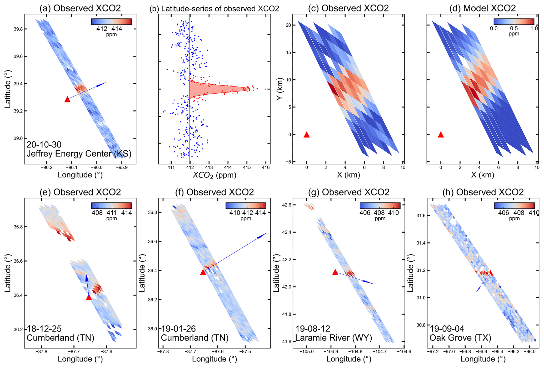
Figure 1Estimation process of power plant emissions (a–d). (a) CO2 plume of the Jeffrey Energy Center power plant on 30 October 2020. (b) Change of XCO2 in a latitude direction from (a). The background value is determined from the average of the observations below the 90th percentile (green line), background points (blue) and plume points (red). (c) Zoomed-in image of (a) in relation to the area of our simulation. (d) The simulated normalized XCO2 enhancement for the same region by the GPM. Panels (e–h) show cases of other power plant emission signals. The blue arrow represents the wind vector halfway the height of the PBL. The wind speeds in (a), (e), (f), (g) and (h) are 2.9, 1.8, 6.1, 2.6 and 3.4 m s−1, respectively.
3.4.2 Time-corrected hourly EPA-reported values
The CO2 emissions released by the power plant are transported to the satellite overpass location by the wind and are detected as XCO2 enhancement. EPA reports the emission value of the power plant on an hourly basis. When comparing emission estimates and hourly reported values, we need to consider the time lag between the moment when the emission is released at the stack and the moment it is detected downwind by the satellite. This time can be calculated from the distance between the power plant and the satellite crossing point and the wind speed. However, unlike the time-weighted reported emission used in Nassar et al. (2021), we use the time that the detected plume was released at the power plant. Therefore, we produce time-corrected hourly reported values at the time of the emissions seen by the satellite overpass instead of reporting the hourly emission values closest to the overpass time.
4.1 Comparison of estimated emissions using hourly monitoring values
Figure 1a shows an example of a power plant emission plume in the satellite observations. The Jeffrey Energy Center power plant in Kansas was in operation at about 01:30 local time on 30 October 2020, and its CO2 plume was captured by the downwind track of OCO-2. The local enhancement appears as a peak in a latitude direction, the cross-section of which is well approximated by a Gaussian (Fig. 1b). For the entire US, we analyzed the 1284 plants reported by the EPA, of which 347 were excluded because of nearby city emissions. A total of 9950 OCO-2 and 13 427 OCO-3 tracks were recorded within a 0.25∘ radius of these power plants. We used observations in the latitude range of ±0.5∘ around the XCO2 maximum for all tracks (the range shown in Fig. 1a) and performed a visual selection to identify cases of enhancement from plumes of isolated power plants like in Fig. 1. The screening criterion is able to select a clear plume profile in the XCO2 observations downwind of the power plant, such as in Fig. 1e–h, while other cases are rejected due to insignificant XCO2 enhancement, missing data and emission source cluster interference, such as in Fig. S10. In the end, we arrived at 50 cases where the power plant was operating and the emission plume crossed the satellite track, including 30 cases from OCO-2 and 20 cases from OCO-3. When the distance between two adjacent power plants did not exceed the range of 1 pixel of the satellite, it was regarded as a single isolated emission source, and their names were connected with commas (Table 1).
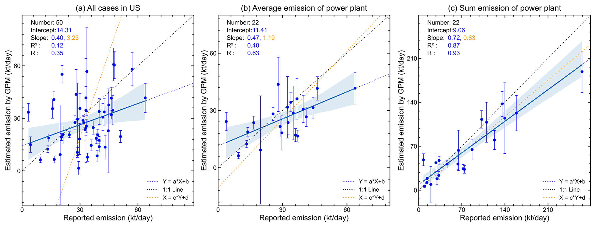
Figure 2The emission estimation results by the GPM of all cases with WPBL are compared with the time-corrected hourly reported value from EPA (a), the average value of emission estimation results of each power plant is compared with the reported value (b), and the sum of emission estimation results of each power plant is compared with the reported value (c). The vertical error line is the total uncertainty of estimated emissions. The yellow and blue dashed lines are the fitted lines with the x axis and y axis swapped.
Previous studies used various choices of wind information to approximately account for the plume spreading, such as the wind speed at the assumed height of the chimney plus an assumed 250 m for typical plume rise above the stack height (Nassar et al., 2021) or 31 m (Chevallier et al., 2020), the average wind speed of the pressure layer near the ground (Zheng et al., 2020a; Hakkarainen et al., 2021), or a calculation of an effective wind (Varon et al., 2018; Reuter et al., 2019; Hakkarainen et al., 2021). In this study, we compared the estimated CO2 emission results driven by WERA5 (Fig. S3), WMERRA (Fig. S4) and WPBL used for the GPM method. The correlation coefficient R of the estimated emission and time-corrected reported US EPA emission of the 50 cases of isolated power plants are 0.35, 0.28 and 0.14 for WPBL, WERA and WMERRA, respectively (Figs. 2a, S3a, S4a). The results show that the emission estimates obtained using WPBL give better results than the other two wind options, which suggests that it represents the spreading of CO2 plumes in the vertical direction more accurately (Figs. 2, S3, S4). The results using MERRA-2 were worse (Fig. S4) due to its low resolution (GMAO, 2015), which cannot provide precise wind information for emission sources. These 50 cases contain multiple observations of 22 isolated power plants. For some power plants, we have multiple observation days. For these cases we have averaged the results. As shown in Fig. 2b, the correlation coefficient R of the averaged estimated emission and the reported emission is 0.63, 0.44 and 0.22, corresponding to WPBL, WERA and WMERRA, respectively (Figs. 2b, S3b, S4b). We also tested the weighted average considering the uncertainty of the estimates and reached the same conclusion that WPBL has the best performance. The improved correlation illustrates the large fraction of randomness in the emission retrieval uncertainty (Chevallier et al., 2022). For the sum of the estimates of the repetitive cases of each power plant, we obtained a better correlation of 0.93, 0.89 and 0.73, corresponding to WPBL, WERA and WMERRA, respectively (Figs. 2c, S3c, S4c). Therefore, we decided to use WPBL for the estimation of power plant emissions. In this study, the background for the cross-sectional flux method is determined by fitting of Eq. (3), while the background for the Gaussian plume model (GPM) method is determined by the 90th percentile showing the lowest error for all cases in Fig. S2a. The difference in background obtained by these two methods is on average small (Fig. S11a) but with a maximum difference of 0.86 ppm and a minimum of 0.004 ppm (Fig. S11b). Under the two background calculation methods, the GPM method has good consistency in the estimation results driven by three wind fields (Fig. S11c–e). With the background computing by Eq. (3), the conclusion that estimated emissions have better accuracy using the WPBL is still valid (Fig. S12).
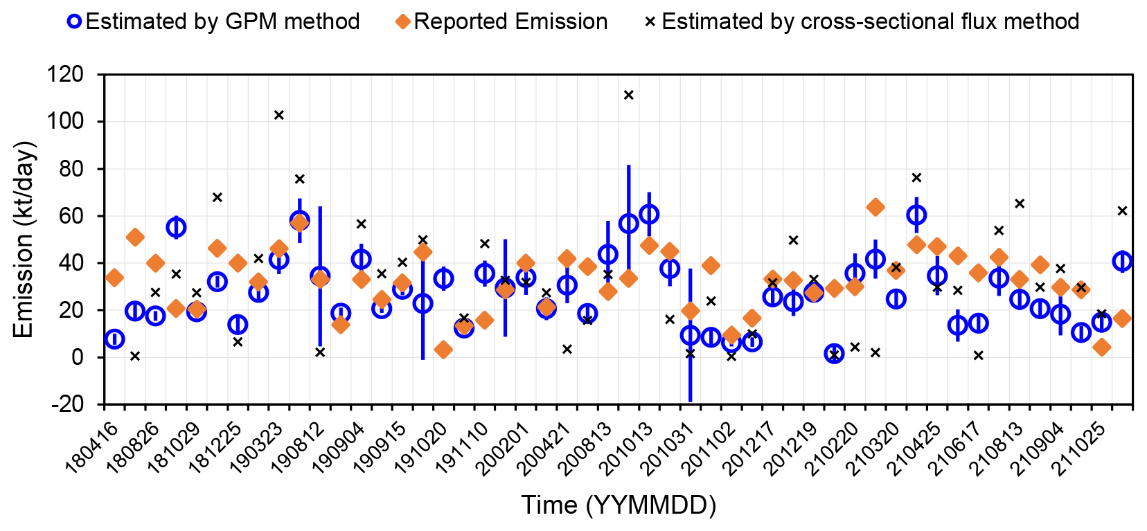
Figure 3Emission values of US power plants estimated with the GPM (blue circles) and cross-sectional flux (black crosses) methods compared to the time-corrected reported values (orange diamonds). The x axis is labeled with YYMMDD.
In Fig. 3, we compare the GPM method and the cross-sectional flux method driven by WPBL. Among them were two cases without a result from the cross-sectional flux method because of invalid fitting. It shows that the estimates from the cross-sectional flux method fluctuate much more than the estimates from the GPM method. This is mainly because the orbits of the OCO-2 and OCO-3 satellites are not perpendicular to the plume, and the final step of the cross-sectional flux method uses the wind field component normal to the orbit multiplied by the line density to estimate the flux, while the GPM method derives the posteriori emission by a linear least-squares fit between observed and simulated enhancements. Moreover, the OCO-2 and OCO-3 observations do not sample the entire emission plume, as shown in Fig. 1f, but just the part of the plume cross-section within the narrow width along the orbit. Hakkarainen et al. (2021) also found that the estimates from the cross-sectional flux method fluctuated greatly. Therefore, we decided to use the GPM method for the estimation of global power plant emissions. When comparing plant-level estimated emission with reported emission by the US Energy Information Administration (EIA) from fuel consumption records (https://www.eia.gov/electricity/data/emissions/, last access: 21 March 2022), Fig. S6 shows that the correlation between estimated emission and reported annual emission from EIA (R=0.39) is lower than that from EPA, although the reported annual emissions from EPA and EIA reveal a good correlation (R=0.80). Figure 4 shows that, due to strong hourly variations in the power plant emission, the satellite overpass time is not always representative of the annual emission of a power plant. Note that EIA reports the yearly mean emission based on the annual fuel consumption of the power plant, which will differ from the emission at the satellite overpass time.
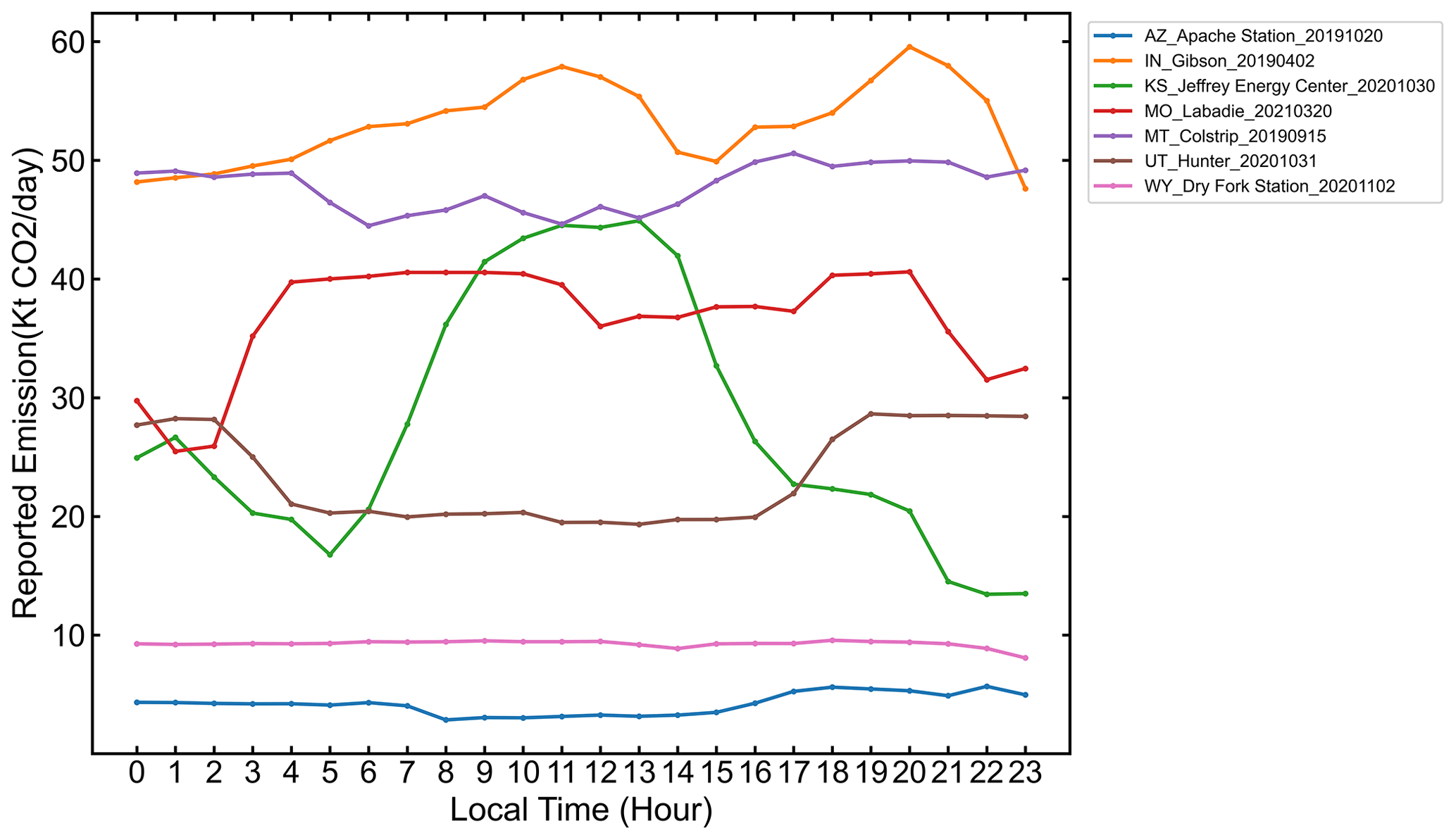
Figure 4Hourly emission variation in seven randomly selected power plants and dates from hourly US EPA data. The name of each curve consists of the name of the state, the name of the power plant and the YYYYMMDD day.
Table 1 lists the average estimated emissions for 22 power plants and the estimated uncertainty caused by the background, XCO2 and wind field. The deviation of the estimated emissions and reported emissions varies between 0.47 and 22.11 kt d−1, and the total uncertainty varies between 1.65 and 28.32 kt d−1. The total uncertainty is comparable to the uncertainty of power plant emissions in previous studies, which ranged from 3.42 to 19.2 kt d−1 (Nassar et al., 2017, 2022). The uncertainty of wind speed is between 0.08 and 1.4 m s−1, and the uncertainty of background varies between 0.03 and 0.1 ppm (Table S1 in the Supplement). Among the three uncertainty components, the uncertainty caused by the wind field is the highest. From 2018 to 2021, for the XCO2 archived data, there are six cases found for the Jeffrey Energy Center power plant (KS) and four cases for the Prairie State Generating Station (IL), Colstrip (MT), Cumberland (TN) and Oak Grove (TX) power plants. For a few power plants, we found that the time variability of estimated and time-corrected hourly EPA-reported emissions from multiple observation cases of power plants displays a good consistency (Fig. S5), such as the Gibson (IN) and Labadie power plants (MO). Excluding the two power plants whose uncertainties are greater than the estimated emissions, the uncertainties of the other cases are within 8 % to 51 % of the reported emissions.
Table 1The average estimated emissions, reported emissions, uncertainty components and number of observations from US power plants.
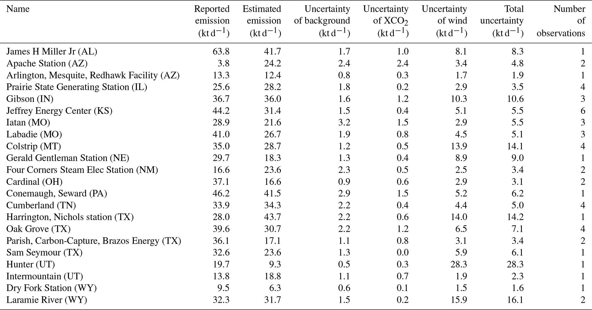
Figure 5 shows the number of cases retained for each processing step of the automatic detection of global power plant emission signals using the GPPD. We obtained 1387 d of XCO2 observation data from OCO-2 from January 2018 to December 2021 and 766 d of XCO2 observation data from OCO-3 from August 2019 to November 2021. For 8660 power plants in the world, all tracks from OCO-2 and OCO-3 were scanned near the power plants. The number of cases with more than 10 observations (step 2 in Sect. 3.3) near the Gaussian peak is 39 365 and 42 932 for OCO-2 and OCO-3. A total of 40.71 % of the XCO2 cases are located in the downwind direction of the power plant. Among them, 24.94 % of cases contain at least five observations that are significantly enhanced relative to the background. Among those 518 and 804 plume observations with at least five observation points from OCO-2 and OCO-3 have net enhancement exceeding 1.5 ppm. Finally, through visual selection (step 6 in Sect. 3.3), 83 and 23 cases from OCO-2 and OCO-3 were regarded as plumes from isolated power plants, respectively.
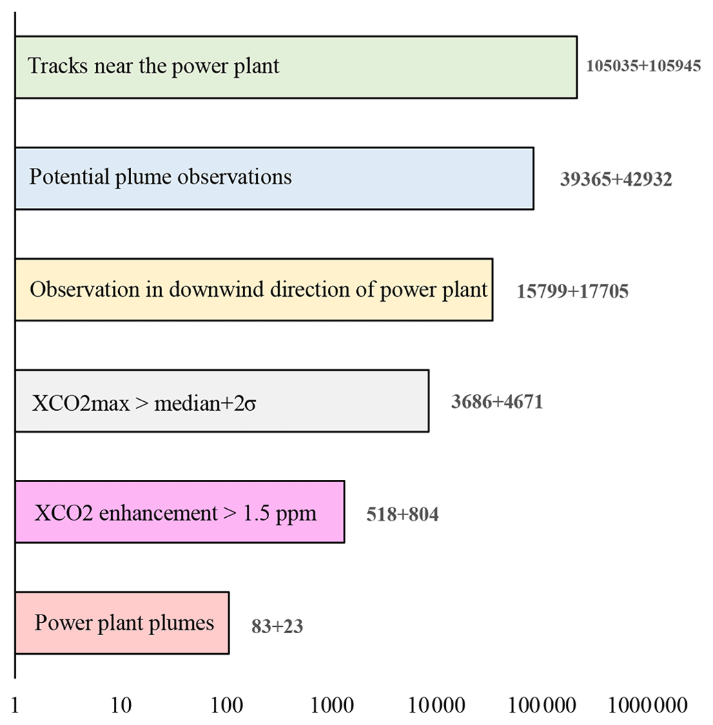
Figure 5Statistics of the number of OCO-2 and OCO-3 XCO2 observations, respectively, in each processing step.
Figure 6 shows the estimated CO2 emissions of 106 global power plant cases calculated by the GPM method using WPBL. The estimated emissions of these power plants range from 3.2 to 109.0 kt d−1. The 25th, 50th and 75th percentiles of the estimated emissions are 19.9, 32.1 and 52.6 kt d−1, respectively. The uncertainties range from 1.2 to 62.6 kt d−1, and the 25th, 50th and 75th percentiles of uncertainty in the estimated emissions are 18 %, 29 % and 50 % (Table S2). Figure 6a shows the location of these power plants and their emissions, indicated by circle size and color. Figure 6b shows the sum of estimated emissions for all observations found at each power plant. The gray vertical lines are an indication of the uncertainty of the estimated emissions. Furthermore, we calculated the correlation between the integral of the observed and simulated XCO2 enhancement from Eqs. (1) and (2) in the latitude direction. Figure S7 shows a correlation coefficient of 0.56 for observed and simulated enhancements of global power plant cases.
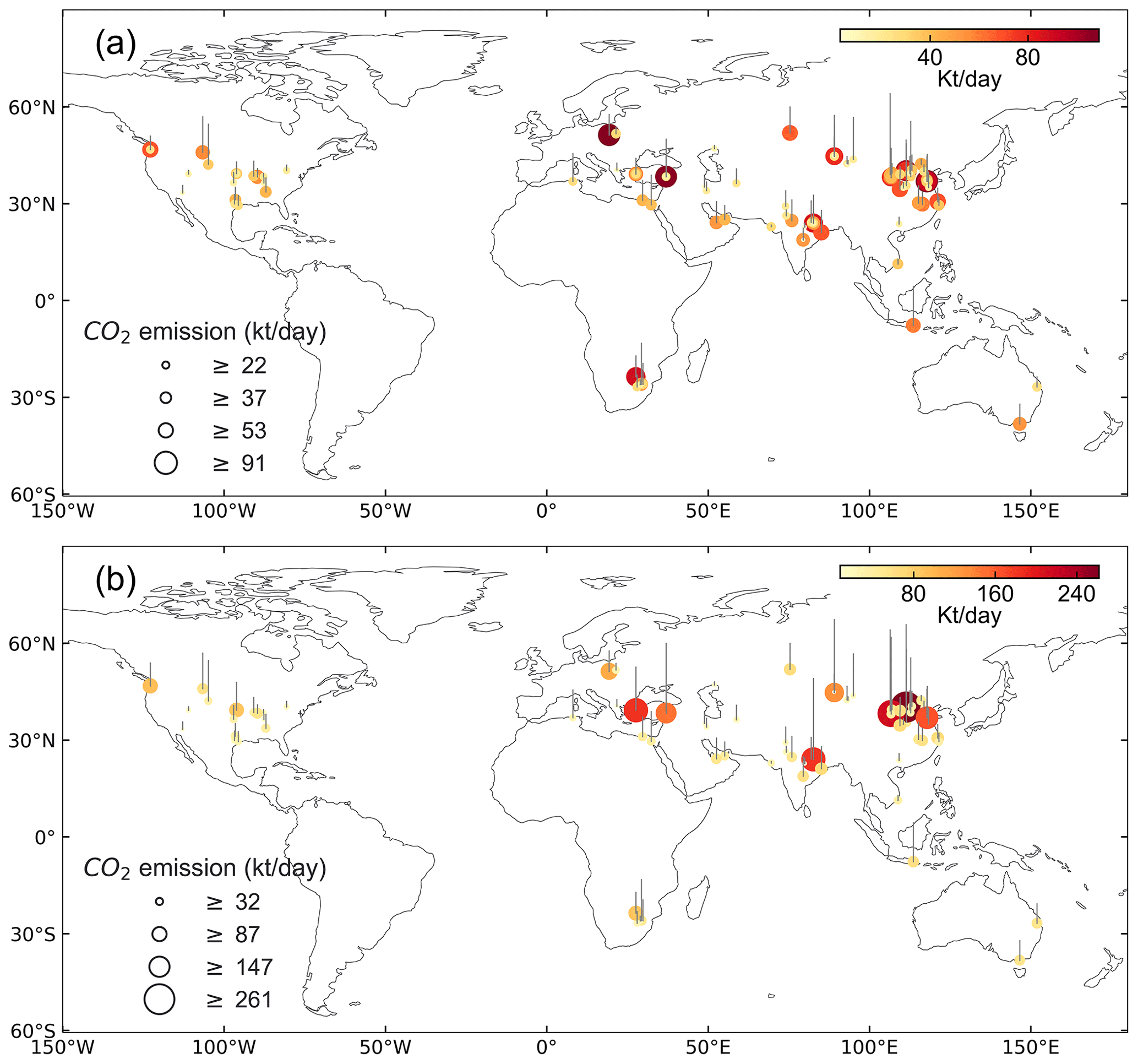
Figure 6The detected global power plants with emission estimation results (a) and the sum of emission estimation results of all found observations at each power plant (b). The gray vertical lines are an indication of the uncertainty of the estimated emissions. The color and size of the circles indicate the estimated emission.
The detection algorithm reduces 4-year global XCO2 data to only 106 cases of 78 unique power plants. A large number of power plant emission cases have been discarded due to insignificant XCO2 enhancements of less than 1.5 ppm, not enough valid observations in the plume and finally by a visual check. We compare the estimated emissions with the carbon emission inventory EDGAR v6.0 for the power sector in order to understand the magnitude of the emissions of detected cases. The estimated emissions of detected power plants are counted by year and country (Fig. 7). When assuming constant emissions of power plants, the sum of estimated emissions of all power plants would be extrapolated to 1522 ± 501 Mt yr−1. According to EDGAR, this value accounts for about 17 % of the power sector 2018 emissions of the countries in Fig. 7b. The estimated emissions from the few observations in 2018, 2019, 2020 and 2021 account for only 2 %, 5 %, 6 % and 4 %, respectively, of all power sector emissions of countries showed in Fig. 7a in 2018. The top three countries in terms of detected estimated emissions of power plants are China, the US and India. This illustrates the fact that OCO-2 and OCO-3 are only capable of seeing a fraction of the emitted CO2 emissions due to the limited spatial coverage of the instrument and the often cloudy conditions during observation.
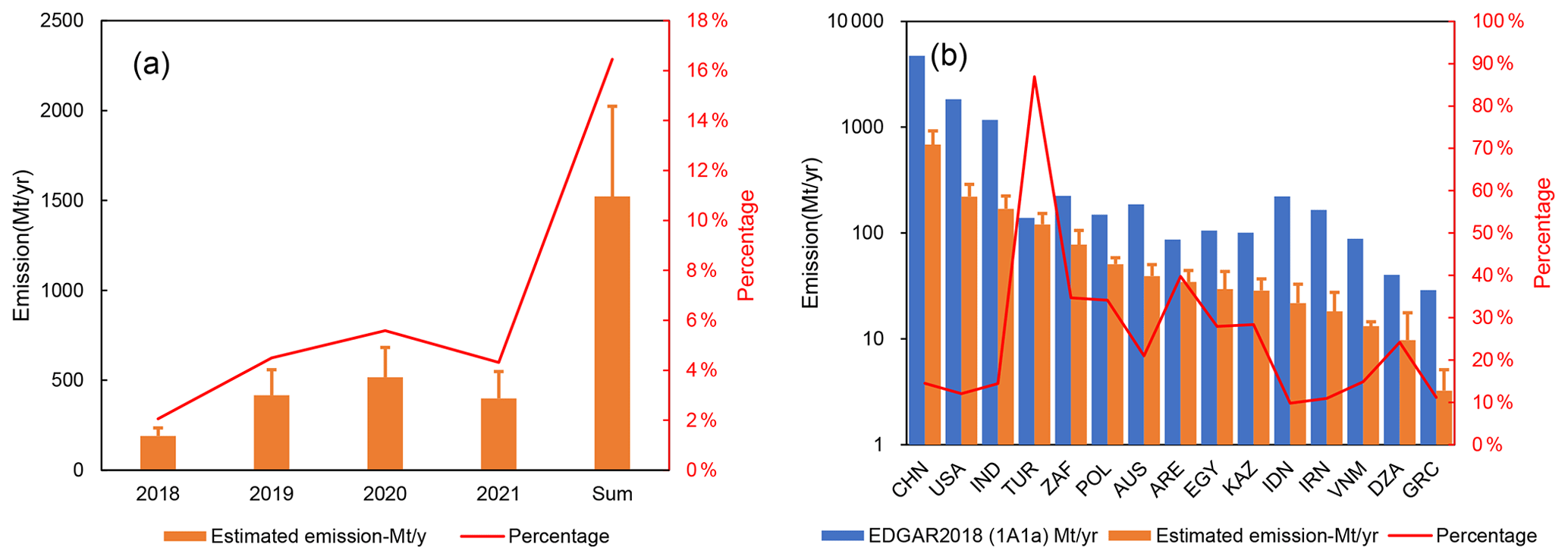
Figure 7Estimated annual emissions of the detected global power plants, also shown as a percentage of the total reported emissions of global power plants. (a) The red curve shows the proportion of annual estimated emissions to the total emissions of all countries with observations in 2018 (from EDGAR2018 v6.0 1A1a). (b) The red curve in the right figure shows the percentage of estimated emissions in comparison to the country's total power plant emissions according to the inventory.
In this study, we compared two widely used methods for estimating point source emissions of power plants: the Gaussian plume model method and cross-sectional flux method. We applied the two methods to carefully selected power plant plumes in the US observed by OCO-2 and OCO-3. The accuracy of the two methods is validated with time-corrected hourly reported emissions from EPA. We found that the cross-sectional flux method has a larger variability than the GPM method. This is because when the angle between the orbit and the wind direction is large, the actual cross-section shape is asymmetric Gaussian. But the resolution of OCO observations is not sufficient to fully fit asymmetric Gaussian curves. However, the GPM method directly simulates XCO2 enhancements at any downwind position using the wind direction of the emission source, avoiding this issue and obtaining more stable results. We used the Gaussian plume model method to evaluate the impact of three kinds of wind field datasets (WPBL, WERA and WMERRA) on the accuracy of emission estimates of isolated power plants. The results show that, for a single case, the correlation between reported emission and estimated emission driven by WPBL is the highest. When there are multiple observations of the same power plant, the correlation between the average and total estimated emissions of the power plant and the reported emissions is significantly improved, from R2=0.40 to 0.87. No matter what kind of wind field data are used, the Gaussian plume model has a high correlation R2 of the total emissions from power plants from multiple observations, which is above 0.5. In general, obtaining more observation data from more instruments can significantly reduce the uncertainty of estimated emissions of power plants.
Once having selected the best emission estimation method for isolated power plants, we applied this simple and fast method globally. We developed a procedure to automatically detect the emission signals of power plants and, after a visual selection, obtained 106 global power plant emission observations of 78 power plants.
Unlike continuous imaging satellites, OCO-2 and OCO-3 scans cover a very limited part of the Earth's surface on a daily basis. By removing the cloud impact and only extracting the downwind emission plumes of power plants, the available observations are further reduced. The extremely limited number of cases from the existing satellites makes it impossible to capture the time variability of power plants, whether diurnal or seasonal. In addition, only isolated emission hotspots are estimated here to avoid the impact of adjacent emission sources.
This study has only considered three sources of uncertainty. Future research may investigate additional sources, such as the assumption of steady-state conditions and the plume rise, to better understand their impact on the results. With the future increase in observation sensors with improved spatial-temporal resolution, such as the planned Copernicus Carbon Dioxide Monitoring mission (CO2M) and the Japanese Global Observing Satellite for Greenhouse gases and Water cycle (GOSAT-GW), the probability of observing a CO2 plume will greatly increase. The abundant observation data obtained by the new generation of satellites will contribute to the monitoring of power plant emissions worldwide. The emissions of power plants in the background of other emission signals may also be monitored due to high-resolution observations and increased swath width, and the uncertainty of the estimated emissions of power plants will further decrease.
Version 10r of OCO-2 and Version 10.4r of OCO-3 bias-corrected XCO2 retrievals was downloaded from the data archive maintained at the NASA Goddard Earth Science Data and Information Services Center (https://doi.org/10.5067/E4E140XDMPO2, OCO-2 Science Team, 2020, https://doi.org/10.5067/970BCC4DHH24, OCO-2/OCO-3 Science Team, 2022). Versions 1.3.2 and 2.2.0 of the TROPOMI L2 offline products were obtained online (https://doi.org/10.5194/amt-15-2037-2022, van Geffen et al., 2022).
The supplement related to this article is available online at: https://doi.org/10.5194/acp-23-6599-2023-supplement.
Conceptualization and methodology: XL, RvdA, JdL, FC, ZL, and PC; data processing: XL, HE, ZD, YG, XS, XN, DH, and XD; model simulation: XL; formal analysis: XL, RvdA, and JdL; writing (original draft): XL; writing (review and editing): all authors; visualization: XL; supervision, project administration, and funding acquisition: ZL.
The contact author has declared that none of the authors has any competing interests.
Publisher’s note: Copernicus Publications remains neutral with regard to jurisdictional claims in published maps and institutional affiliations.
The support provided by the China Scholarship Council (CSC) during a visit by Xiaojuan Lin to the Royal Netherlands Meteorological Institute (KNMI) is acknowledged.
This research has been supported by the National Natural Science Foundation of China (grant nos. 71874097, 41921005, 71904007 and 71904104).
This paper was edited by Eduardo Landulfo and reviewed by Ray Nassar and Gerrit Kuhlmann.
IEA: CO2 Emissions from Fuel Combustion 2019, IEA, Paris, https://doi.org/10.1787/2a701673-en, [data set], 2019.
Beirle, S., Borger, C., Dörner, S., Eskes, H., Kumar, V., de Laat, A., and Wagner, T.: Catalog of NOx emissions from point sources as derived from the divergence of the NO2 flux for TROPOMI, Earth Syst. Sci. Data, 13, 2995–3012, https://doi.org/10.5194/essd-13-2995-2021, 2021.
Bovensmann, H., Buchwitz, M., Burrows, J. P., Reuter, M., Krings, T., Gerilowski, K., Schneising, O., Heymann, J., Tretner, A., and Erzinger, J.: A remote sensing technique for global monitoring of power plant CO2 emissions from space and related applications, Atmos. Meas. Tech., 3, 781–811, https://doi.org/10.5194/amt-3-781-2010, 2010.
Broquet, G., Bréon, F.-M., Renault, E., Buchwitz, M., Reuter, M., Bovensmann, H., Chevallier, F., Wu, L., and Ciais, P.: The potential of satellite spectro-imagery for monitoring CO2 emissions from large cities, Atmos. Meas. Tech., 11, 681–708, https://doi.org/10.5194/amt-11-681-2018, 2018.
CEOS: “Pilot Top-down Carbon Dioxide and Methane Budgets” from https://ceos.org/gst/ghg.html last access: 11 October 2022, 2022.
Chevallier, F., Broquet, G., Zheng, B., Ciais, P., and Eldering, A.: Large CO2 Emitters as Seen From Satellite: Comparison to a Gridded Global Emission Inventory, Geophys. Res. Lett., 49, e2021GL097540, https://doi.org/https://doi.org/10.1029/2021GL097540, 2022.
Chevallier, F., Zheng, B., Broquet, G., Ciais, P., Liu, Z., Davis, S. J., Deng, Z., Wang, Y., Breon, F. M., and O'Dell, C. W.: Local anomalies in the column-averaged dry air mole fractions of carbon dioxide across the globe during the first months of the coronavirus recession, Geophys. Res. Lett., e2020GL090244, https://doi.org/10.1029/2020GL090244, 2020.
Crippa, M., Solazzo, E., Huang, G. L., Guizzardi, D., Koffi, E., Muntean, M., Schieberle, C., Friedrich, R., and Janssens-Maenhout, G.: High resolution temporal profiles in the Emissions Database for Global Atmospheric Research, Sci. Data, 7, 121, https://doi.org/10.1038/s41597-020-0462-2, 2020.
Crisp, D., Pollock, H. R., Rosenberg, R., Chapsky, L., Lee, R. A. M., Oyafuso, F. A., Frankenberg, C., O'Dell, C. W., Bruegge, C. J., Doran, G. B., Eldering, A., Fisher, B. M., Fu, D., Gunson, M. R., Mandrake, L., Osterman, G. B., Schwandner, F. M., Sun, K., Taylor, T. E., Wennberg, P. O., and Wunch, D.: The on-orbit performance of the Orbiting Carbon Observatory-2 (OCO-2) instrument and its radiometrically calibrated products, Atmos. Meas. Tech., 10, 59–81, https://doi.org/10.5194/amt-10-59-2017, 2017.
Engelen, R.: The Copernicus anthropogeni CO2 emissions Monitoring and Verification Support capacity – a brief overview, the CoCO2 Consortium, https://www.coco2-project.eu/sites/default/files/2021-11/REPORT%20Copernicus%20CO2MVS%20description.pdf (last access: 20 September 2022), 2021.
European, C., Joint Research, C., Monforti-Ferrario, F., Oreggioni, G., Schaaf, E., Guizzardi, D., Olivier, J., Solazzo, E., Lo Vullo, E., Crippa, M., Muntean, M., and Vignati, E.: Fossil CO2 and GHG emissions of all world countries: 2019 report, Publications Office, https://data.europa.eu/doi/10.2760/687800 (last access: 2 May 2022), 2019.
Gilfillan, D. and Marland, G.: CDIAC-FF: global and national CO2 emissions from fossil fuel combustion and cement manufacture: 1751–2017, Earth Syst. Sci. Data, 13, 1667–1680, https://doi.org/10.5194/essd-13-1667-2021, 2021.
GMAO: MERRA-2 tavg1_2d_slv_Nx: 2d,1-Hourly,Time-Averaged,Single-Level,Assimilation,Single-Level Diagnostics V5.12.4, https://disc.gsfc.nasa.gov/datasets/M2T1NXSLV_5.12.4/summary (last access: 26 March 2022), 2015.
Hakkarainen, J., Ialongo, I., Maksyutov, S., and Crisp, D.: Analysis of Four Years of Global XCO2 Anomalies as Seen by Orbiting Carbon Observatory-2, Remote Sens., 11, 850, https://doi.org/10.3390/rs11070850, 2019.
Hakkarainen, J., Szeląg, M. E., Ialongo, I., Retscher, C., Oda, T. and Crisp, D.: Analyzing nitrogen oxides to carbon dioxide emission ratios from space: A case study of Matimba Power Station in South Africa, Atmos. Environ.: 10, 100110, https://doi.org/10.1016/j.aeaoa.2021.100110, 2021.
Hill, T. and Nassar, R.: Pixel Size and Revisit Rate Requirements for Monitoring Power Plant CO2 Emissions from Space, Remote Sens., 11, 1608, https://doi.org/10.3390/rs11131608, 2019.
IPCC: Summary for Policymakers, Climate Change 2021: The Physical Science Basis, in: Contribution of Working Group I to the Sixth Assessment Report of the Intergovernmental Panel on Climate Change, edited by: Masson-Delmotte, V., Zhai, P., Pirani, A., Connors, S. L., Péan, C., Berger, S., Caud, N., Chen, Y., Goldfarb, L., Gomis, M. I., Huang, M., Leitzell, K., Lonnoy, E., Matthews, J. B. R., Maycock, T. K., Waterfield, T., Yelekçi, O., Yu, R., and Zhou, B., Cambridge, United Kingdom and New York, NY, USA, Cambridge University Press., 3–32, https://doi.org/10.1017/9781009157896.001, 2021.
Janardanan, R., Maksyutov, S., Oda, T., Saito, M., Kaiser, J. W., Ganshin, A., Stohl, A., Matsunaga, T., Yoshida, Y., and Yokota, T.: Comparing GOSAT observations of localized CO2 enhancements by large emitters with inventory-based estimates, Geophys. Res. Lett., 43, 3486–3493, https://doi.org/10.1002/2016gl067843, 2016.
Kiel, M., Eldering, A., Roten, D. D., Lin, J. C., Feng, S., Lei, R., Lauvaux, T., Oda, T., Roehl, C. M., Blavier, J.-F., and Iraci, L. T.: Urban-focused satellite CO2 observations from the Orbiting Carbon Observatory-3: A first look at the Los Angeles megacity, Remote Sens. Environ., 258, 112314, https://doi.org/10.1016/j.rse.2021.112314, 2021.
Kuhlmann, G., Broquet, G., Marshall, J., Clément, V., Löscher, A., Meijer, Y., and Brunner, D.: Detectability of CO2 emission plumes of cities and power plants with the Copernicus Anthropogenic CO2 Monitoring (CO2M) mission, Atmos. Meas. Tech., 12, 6695–6719, https://doi.org/10.5194/amt-12-6695-2019, 2019.
Kuhlmann, G., Henne, S., Meijer, Y., and Brunner, D.: Quantifying CO2 Emissions of Power Plants With CO2 and NO2 Imaging Satellites, Front. Remote Sens., 2, 14, https://doi.org/10.3389/frsen.2021.689838, 2021.
Kunik, L., Mallia, D. V., Gurney, K. R., Mendoza, D. L., Oda, T., and Lin, J. C.: Bayesian inverse estimation of urban CO2 emissions: Results from a synthetic data simulation over Salt Lake City, UT, Elementa, 7, 36, https://doi.org/10.1525/elementa.375, 2019.
Lauvaux, T., Giron, C., Mazzolini, M., d'Aspremont, A., Duren, R., Cusworth, D., Shindell, D., and Ciais, P.: Global assessment of oil and gas methane ultra-emitters, Science, 375, 557–561, https://doi.org/10.1126/science.abj4351, 2022.
NASA: CMS-Relevant Missions, https://carbon.nasa.gov/missions.html#sub (last access: 26 August 2022), 2022.
Nassar, R., Hill, T. G., McLinden, C. A., Wunch, D., Jones, D. B. A., and Crisp, D.: Quantifying CO2 Emissions From Individual Power Plants From Space, Geophys. Res. Lett., 44, 10045–10053, https://doi.org/10.1002/2017gl074702, 2017.
Nassar, R., Mastrogiacomo, J.-P., Bateman-Hemphill, W., McCracken, C., MacDonald, C. G., Hill, T., O'Dell, C. W., Kiel, M., and Crisp, D.: Advances in quantifying power plant CO2 emissions with OCO-2, Remote Sens. Environ., 264, 112579, https://doi.org/10.1016/j.rse.2021.112579, 2021.
Nassar, R., Moeini, O., Mastrogiacomo, J.-P., O'Dell, C. W., Nelson, R. R., Kiel, M., Chatterjee, A., Eldering, A., and Crisp, D.: Tracking CO2 emission reductions from space: A case study at Europe's largest fossil fuel power plant, Front. Remote Sens., 3, 1028240, https://doi.org/10.3389/frsen.2022.1028240, 2022.
O'Brien, D. M., Polonsky, I. N., Utembe, S. R., and Rayner, P. J.: Potential of a geostationary geoCARB mission to estimate surface emissions of CO2, CH4 and CO in a polluted urban environment: case study Shanghai, Atmos. Meas. Tech., 9, 4633–4654, https://doi.org/10.5194/amt-9-4633-2016, 2016.
OCO-2 Science Team: Michael Gunson, Annmarie Eldering: OCO-2 Level 2 bias-corrected XCO2 and other select fields from the full-physics retrieval aggregated as daily files, Retrospective processing V10r, Greenbelt, MD, USA, Goddard Earth Sciences Data and Information Services Center (GES DISC), [data set], https://doi.org/10.5067/E4E140XDMPO2, 2020.
OCO-2/OCO-3 Science Team: Abhishek Chatterjee, Vivienne Payne (2022), OCO-3 Level 2 bias-corrected XCO2 and other select fields from the full-physics retrieval aggregated as daily files, Retrospective processing v10.4r, Greenbelt, MD, USA, Goddard Earth Sciences Data and Information Services Center (GES DISC), [data set], https://doi.org/10.5067/970BCC4DHH24, 2022.
O'Dell, C. W., Eldering, A., Wennberg, P. O., Crisp, D., Gunson, M. R., Fisher, B., Frankenberg, C., Kiel, M., Lindqvist, H., Mandrake, L., Merrelli, A., Natraj, V., Nelson, R. R., Osterman, G. B., Payne, V. H., Taylor, T. E., Wunch, D., Drouin, B. J., Oyafuso, F., Chang, A., McDuffie, J., Smyth, M., Baker, D. F., Basu, S., Chevallier, F., Crowell, S. M. R., Feng, L., Palmer, P. I., Dubey, M., García, O. E., Griffith, D. W. T., Hase, F., Iraci, L. T., Kivi, R., Morino, I., Notholt, J., Ohyama, H., Petri, C., Roehl, C. M., Sha, M. K., Strong, K., Sussmann, R., Te, Y., Uchino, O., and Velazco, V. A.: Improved retrievals of carbon dioxide from Orbiting Carbon Observatory-2 with the version 8 ACOS algorithm, Atmos. Meas. Tech., 11, 6539–6576, https://doi.org/10.5194/amt-11-6539-2018, 2018.
Oda, T., Maksyutov, S., and Andres, R. J.: The Open-source Data Inventory for Anthropogenic CO2, version 2016 (ODIAC2016): a global monthly fossil fuel CO2 gridded emissions data product for tracer transport simulations and surface flux inversions, Earth Syst. Sci. Data, 10, 87–107, https://doi.org/10.5194/essd-10-87-2018, 2018.
Olivier, J. G., Schure, K., and Peters, J.: Trends in global CO2 and total greenhouse gas emissions, PBL Netherlands Environmental Assessment Agency, 5, 1–11, 2017.
Pasquill, F.: The Estimation of the Dispersion of Windborne Material, Meteorol Mag., 90, 33–49, 1961.
Reuter, M., Buchwitz, M., Schneising, O., Krautwurst, S., O'Dell, C. W., Richter, A., Bovensmann, H., and Burrows, J. P.: Towards monitoring localized CO2 emissions from space: co-located regional CO2 and NO2 enhancements observed by the OCO-2 and S5P satellites, Atmos. Chem. Phys., 19, 9371–9383, https://doi.org/10.5194/acp-19-9371-2019, 2019.
Shekhar, A., Chen, J., Paetzold, J. C., Dietrich, F., Zhao, X., Bhattacharjee, S., Ruisinger, V., and Wofsy, S. C.: Anthropogenic CO2 emissions assessment of Nile Delta using XCO2 and SIF data from OCO-2 satellite, Environ. Res. Lett., 15, 095010, https://doi.org/10.1088/1748-9326/ab9cfe, 2020.
UNFCCC: Decision 18/CMA.1 Modalities, procedures and guidelines for the transparency framework for action and support referred to in Article 13 of the Paris Agreement, FCCC/PA/CMA/2018/Add.2, https://unfccc.int/sites/default/files/resource/cma2018_3_add2_new_advance.pdf (last access: 2 May 2022), 2018.
Varon, D. J., Jacob, D. J., McKeever, J., Jervis, D., Durak, B. O. A., Xia, Y., and Huang, Y.: Quantifying methane point sources from fine-scale satellite observations of atmospheric methane plumes, Atmos. Meas. Tech., 11, 5673–5686, https://doi.org/10.5194/amt-11-5673-2018, 2018.
van Geffen, J., Eskes, H., Compernolle, S., Pinardi, G., Verhoelst, T., Lambert, J.-C., Sneep, M., ter Linden, M., Ludewig, A., Boersma, K. F., and Veefkind, J. P.: Sentinel-5P TROPOMI NO2 retrieval: impact of version v2.2 improvements and comparisons with OMI and ground-based data, [data set], Atmos. Meas. Tech., 15, 2037–2060, https://doi.org/10.5194/amt-15-2037-2022, 2022.
Velazco, V. A., Buchwitz, M., Bovensmann, H., Reuter, M., Schneising, O., Heymann, J., Krings, T., Gerilowski, K., and Burrows, J. P.: Towards space based verification of CO2 emissions from strong localized sources: fossil fuel power plant emissions as seen by a CarbonSat constellation, Atmos. Meas. Tech., 4, 2809–2822, https://doi.org/10.5194/amt-4-2809-2011, 2011.
Wang, Y., Broquet, G., Bréon, F.-M., Lespinas, F., Buchwitz, M., Reuter, M., Meijer, Y., Loescher, A., Janssens-Maenhout, G., Zheng, B., and Ciais, P.: PMIF v1.0: assessing the potential of satellite observations to constrain CO2 emissions from large cities and point sources over the globe using synthetic data, Geosci. Model Dev., 13, 5813–5831, https://doi.org/10.5194/gmd-13-5813-2020, 2020.
Wu, D., Lin, J. C., Oda, T., and Kort, E. A.: Space-based quantification of per capita CO2 emissions from cities, Environ. Res. Lett., 15, 035004, https://doi.org/10.1088/1748-9326/ab68eb, 2020.
Ye, X., Lauvaux, T., Kort, E. A., Oda, T., Feng, S., Lin, J. C., Yang, E. G., and Wu, D.: Constraining Fossil Fuel CO2 Emissions From Urban Area Using OCO2 Observations of Total Column CO2, J. Geophys. Res.-Atmos., 125, e2019JD030528, https://doi.org/10.1029/2019jd030528, 2020.
Yin, L., Byers, L., Valeri, L. M., and Friedrich, J.: Estimating Power Plant Generation in the Global Power Plant Database, https://datasets.wri.org/dataset/globalpowerplantdatabase (last access: 2 June 2021), 2021.
Zheng, B., Tong, D., Li, M., Liu, F., Hong, C., Geng, G., Li, H., Li, X., Peng, L., Qi, J., Yan, L., Zhang, Y., Zhao, H., Zheng, Y., He, K., and Zhang, Q.: Trends in China's anthropogenic emissions since 2010 as the consequence of clean air actions, Atmos. Chem. Phys., 18, 14095–14111, https://doi.org/10.5194/acp-18-14095-2018, 2018.
Zheng, B., Chevallier, F., Ciais, P., Broquet, G., Wang, Y., Lian, J., and Zhao, Y.: Observing carbon dioxide emissions over China's cities and industrial areas with the Orbiting Carbon Observatory-2, Atmos. Chem. Phys., 20, 8501–8510, https://doi.org/10.5194/acp-20-8501-2020, 2020a.
Zheng, B., Geng, G. N., Ciais, P., Davis, S. J., Martin, R. V., Meng, J., Wu, N. N., Chevallier, F., Broquet, G., Boersma, F., van der Ronald, A., Lin, J. T., Guan, D. B., Lei, Y., He, K. B., and Zhang, Q.: Satellite-based estimates of decline and rebound in China's CO2 emissions during COVID-19 pandemic, Sci. Adv., 6, eabd4998, https://doi.org/10.1126/sciadv.abd4998, 2020b.
Zheng, T., Nassar, R., and Baxter, M.: Estimating power plant CO2 emission using OCO-2 XCO2 and high resolution WRF-Chem simulations, Environ. Res. Lett., 14, 085001, https://doi.org/10.1088/1748-9326/ab25ae, 2019.