Antarctic atmospheric Richardson number from radiosonde measurements and AMPS

Monitoring a wide range of atmospheric turbulence over the Antarctic continent is still tricky, while the atmospheric Richardson number (Ri; a valuable parameter which determines the possibility that turbulence could be triggered) is easier to obtain. The Antarctic atmospheric Ri, calculated from the potential temperature and wind speed, was investigated using the daily results from the radiosoundings and forecasts of the Antarctic Mesoscale Prediction System (AMPS). Radiosoundings for a year at three sites (McMurdo – MM, South Pole – SP, and Dome C – DC) were used to quantify the reliability of the AMPS forecasts. The AMPS-forecasted Ri can identify the main spatiotemporal characteristics of atmospheric turbulence over the Antarctic region. The correlation coefficients (R_xy) of log ₁₀(Ri) at McMurdo, the South Pole, and Dome C are 0.71, 0.59, and 0.53, respectively. The Ri was generally underestimated by the AMPS and the AMPS could better capture the trend of log ₁₀(Ri) at relatively unstable atmospheric conditions. The seasonal median of log ₁₀(Ri) along two vertical cross-sections of the AMPS forecasts are presented, and it shows some zones where atmospheric turbulence can be highly triggered in Antarctica. The Ri distributions appear to be reasonably correlated to some large-scale phenomena or local-scale dynamics (katabatic winds, polar vortices, convection, gravity wave, etc.) over the Antarctic plateau and surrounding ocean. Finally, the log ₁₀(Ri) at the planetary boundary layer height (PBLH) were calculated and their median value is 0.316. This median value, in turn, was used to estimate the PBLH and agrees well with the AMPS-forecasted PBLH (R_xy>0.69). Overall, our results suggest that the Ri estimated by AMPS are reasonable and the turbulence conditions in Antarctica are well revealed.

1 Introduction

The Richardson number (Ri) is a valuable parameter for giving insight into atmospheric stability; it combines both thermodynamic and dynamic profiles, which can indirectly characterize turbulent heat fluxes (Town and Walden, 2009) and optical turbulence (Yang et al., 2021, 2022) in Antarctica. However, the measurements of atmospheric properties in Antarctica are sparse compared to those in the mid-latitudes and tropics. Atmospheric models have been developed to overcome this limitation (Meso-NH by Lascaux et al., 2009; Polar WRF by Bromwich et al., 2013; MAR by Gallée et al., 2015), allowing researchers to investigate atmospheric variability beyond observational coverage, even for forecasting atmospheric parameters in the future. The Antarctic Mesoscale Prediction System (AMPS; https://www2.mmm.ucar.edu/rt/amps/, last access: 1 March 2022) runs a real-time atmospheric model and provides numerical forecasts for Antarctica. The performances of AMPS in forecasting temperature, wind, precipitable water vapor, cloud, radiation, and heat flux have been examined in previous studies (Monaghan et al., 2005; Seefeldt et al., 2011; Vázquez B and Grejner-Brzezinska, 2012; Wille et al., 2016; Listowski and Lachlan-Cope, 2017; Hines et al., 2019). To our knowledge, using the AMPS to forecast Ri has not been formally validated. Thus, this study will investigate the reliability of the estimated Ri using AMPS forecasts. The atmospheric model employed for AMPS is the Polar version of the Weather Research and Forecasting (Polar WRF) model (Powers et al., 2012). The Polar WRF (http://polarmet.osu.edu/PWRF/, last access: 1 March 2022) has been modified for use in polar regions, for example, improving the representation of heat transfer through snow and ice (Hines and Bromwich, 2008; Hines et al., 2015). The Polar WRF has been used to simulate the Ri at Dome A (DA) in Antarctica, and the simulated Ri behaved as expected since the Ri is generally large when the disturbance effects of atmospheric turbulence on wave propagation (optical turbulence) are weak (Yang et al., 2021). Besides, the simulated Ri of the Polar WRF performed well in estimating boundary layer height when compared with other methods (Yang et al., 2022).

Presently, monitoring a wide range of atmospheric turbulence over the Antarctic continent is tremendously difficult, but atmospheric Ri is easier to obtain, as it can be calculated from the routine meteorological parameters (potential temperature and wind speed). However, few studies have evaluated atmospheric models to forecast Ri in Antarctica, because of limited meteorological experiments here. Nevertheless, Geissler and Masciadri (2006) and Hagelin et al. (2008) used the European Centre for Medium-Range Weather Forecasts (ECMWF) analyses to calculate the atmospheric Ri in Antarctica. The ECMWF analyses were generated from the data assimilation using observations (Lönnberg and Shaw, 1992) and can provide initial states for numerical models (such as Polar WRF). However, their research has some specific shortcomings (or problems that need further study): (1) They did not compare Ri estimations from forecasts and measurements, while the forecast function is of great significance for practical application (e.g., astronomical observations, aviation safety, optical communication). (2) How model errors of Ri depend on atmospheric conditions has not been analyzed. (3) The correlations between turbulence conditions (indicated by Ri) and some large-scale phenomena or local-scale dynamics in Antarctica were not fully investigated. (4) A reference standard for judging the probability of triggering turbulence using the model-estimated Ri was not given. To fill these gaps, the scientific goals of this paper are thus as follows:

1. To carry out a detailed comparison of potential temperature and wind speed (on which Ri depends) in the atmospheric column, this study extends the model evaluations above two sites (Hagelin et al., 2008) to three sites (McMurdo – MM, South Pole – SP, and Dome C – DC) over the Antarctic continent for an entire year. The three sites are considered representative, as the coast (McMurdo), flank (South Pole), and summit (Dome C) of the Antarctic continent will be compared using radiosoundings and AMPS forecasts.

2. The radiosonde can measure meteorological parameters, which can estimate Ri. Using the AMPS-forecasted meteorological parameters, one also can obtain the Ri. Then, a comparison of Ri estimated from measurements and forecasts can be achieved, allowing us to evaluate the reliability of AMPS-forecasted Ri in giving insight into the atmospheric turbulence in Antarctica. In addition, we investigated how the discrepancies between the models and measurements depend on the atmospheric conditions.

3. Two vertical cross-sections for Ri will be given, which may provide a better perspective on the turbulence conditions in both vertical and horizontal dimensions, instead of only focusing on the vertical dimension (or atmospheric column; e.g.,  Geissler and Masciadri, 2006; Hagelin et al., 2008). This will help to identify regions and periods that are favorable for triggering atmospheric turbulence in Antarctica. Moreover, this will enable us to correlate the Ri distribution with some large-scale phenomena or local-scale dynamics (katabatic winds, polar vortices, convection, gravity wave, etc.) in Antarctica, and the underlying physical processes of Antarctic atmospheric turbulence will be investigated.

4. The planetary boundary layer height (PBLH, within which the atmosphere is generally turbulent) can be estimated using a critical value of Ri, typically 0.25 (Holtslag et al., 1990; Pietroni et al., 2012; Petenko et al., 2019). However, this critical value depends on the vertical resolution of data (Troen and Mahrt, 1986; Holtslag et al., 1990) and may be different for the AMPS grid resolution. Then the Ri at the AMPS-forecasted PBLH (Ri_PBLH) was obtained as a reference standard for judging whether the atmosphere is likely to be laminar flow (Ri > Ri_PBLH) or turbulent flow (Ri < Ri_PBLH) when using the AMPS-forecasted Ri.

In Sect. 2, we present the experimental data and atmospheric model used in this study, with an explanation of their main features. In Sect. 3, the Ri is introduced. In Sect. 4, we compare AMPS forecasts to radiosoundings and analyze the atmospheric turbulence conditions in Antarctica. Section 5 summarizes the main findings and primary takeaways of this study.

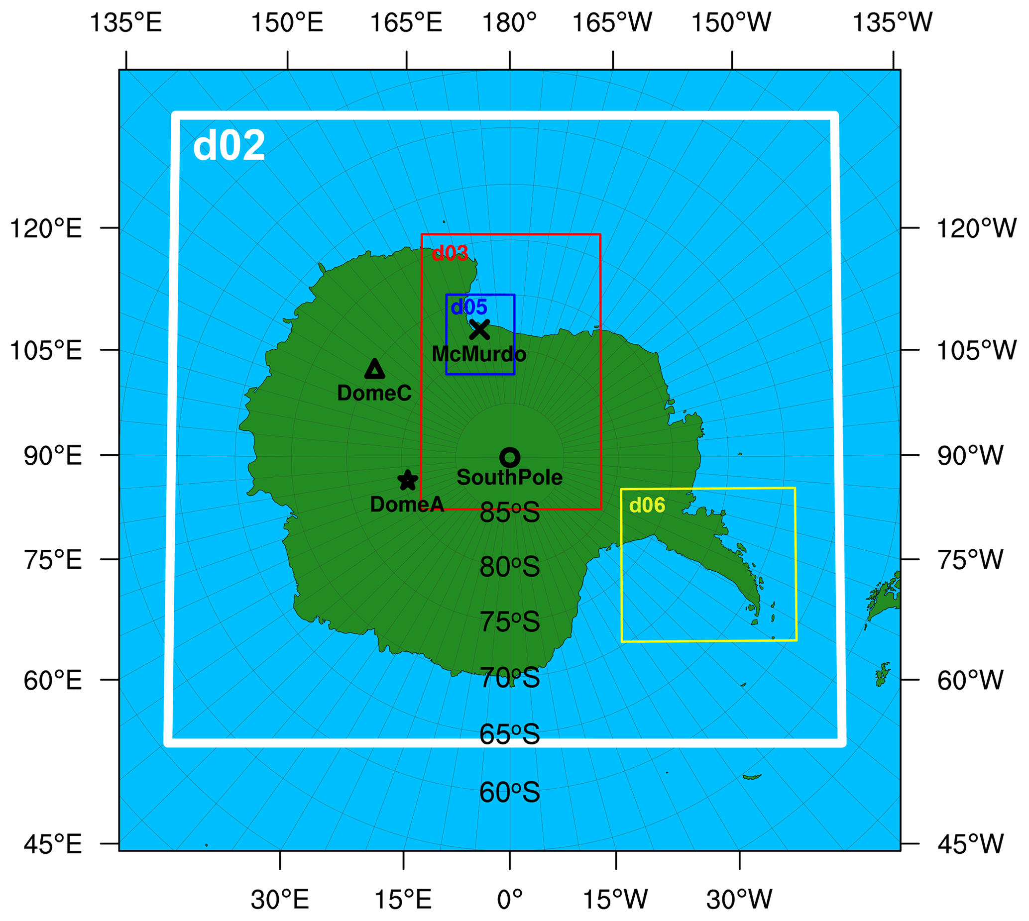
Figure 1 The five two-way interactive horizontal grids (d01, d02, d03, d05, and d06; information online at https://www2.mmm.ucar.edu/rt/amps/information/configuration/maps_2017101012/maps.html, last access: 1 March 2022) used in the AMPS configuration. The locations of McMurdo (78^∘ S, 167^∘ E), South Pole (90^∘ S, …^∘ E), Dome C (75^∘ S, 123^∘ E), and Dome A (80^∘ S, 78^∘ E) are shown by the cross, circle, triangle, and star, respectively.

2 Data and model

2.1 Radiosoundings

Daily radiosounding measurements at McMurdo (MM) and the South Pole (SP) are available at the Antarctic Meteorological Research Center (AMRC; ftp://amrc.ssec.wisc.edu/pub, last access: 1 March 2022). For Dome C (DC), one can obtain the measurements at the Antarctic Meteo-Climatological Observatory (http://www.climantartide.it, last access: 1 March 2022). The altitudes of the three sites are 9 m (MM), 2839 m (SP), and 3239 m (DC), where the altitudes correspond to the heights of the radiosondes at the time of launch. Their locations are shown in Fig. 1. Dome A (DA) is also marked in Fig. 1, which is the highest location (4083 m) on the Antarctic plateau and the atmospheric conditions above it will also be analyzed in this study (see Sect. 4.2.3). The radiosonde-measured meteorological parameters include pressure, temperature, wind speed, and wind direction; 1 year (from March 2021 to February 2022) of these meteorological parameters was used in this study. Generally, the radiosonde was launched once a day at the same hour (sometimes twice a day at MM and SP). In total, 518, 508, and 340 profiles were available at MM, SP, and DC from March 2021 to February 2022.

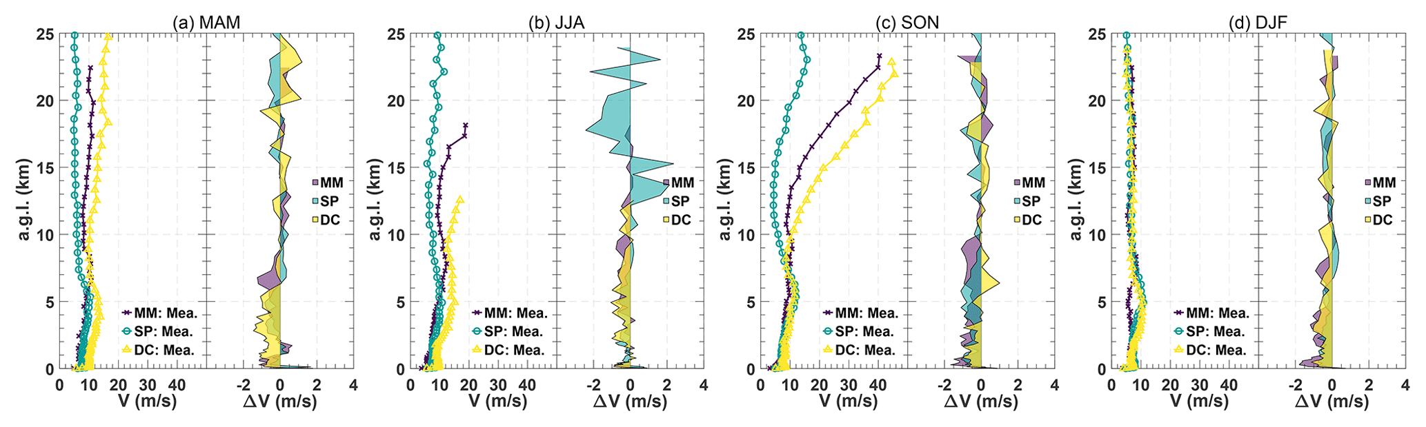
Table 1 Main technical specifications of the radiosonde RS41.

^∗ Resolution in the files that are available for download from the web (ftp://amrc.ssec.wisc.edu/pub, last access: 1 March 2022, http://www.climantartide.it, last access: 1 March 2022).

The radiosonde instrumentation used during this measurement period was the Vaisala RS41 (Technical data: https://www.vaisala.com/en/products/weather-environmental-sensors/upper-air-radiosondes-rs41, last access: 1 March 2022). The accuracy and uncertainty of the radiosonde measurements are listed in Table 1. The radiosondes measure the atmosphere between the ground and an altitude of 10–25 km (low in winter and high in summer) with a typical ascent rate of 5 m s⁻¹ and a logging frequency of 1 Hz; then the vertical resolution is approximately 5 m.

2.2 AMPS

The AMPS can forecast meteorological parameters in four-dimensional space-time in Antarctica, which can be used for comparison with the radiosonde measurements. The AMPS grid system consisted of a series of nested domains with 60 vertical levels. This study used grid 2 fields (d02; 8 km horizontal resolution) that covered the entire Antarctic continent (similar to Hines et al., 2019), as shown by the white square in Fig. 1. However, the contributions from the nested grids with higher horizontal resolutions (d03: 2.67 km; d05: 0.89 km; d06: 2.67 km) are not entirely lost, as the AMPS used a two-way nested run and the nest (e.g., d03) feeds its calculation back to the coarser domain (e.g., d02). The original WRF output files for each AMPS grid were saved in a rolling archive (one can find the steps for downloading the original WRF output files at https://www2.mmm.ucar.edu/rt/amps/information/amps_esg_data_info.html, last access: 1 March 2022). This study used the AMPS outputs (in original WRF format) from the daily AMPS forecasts that began at 12:00 UTC. Parish and Waight (1987) showed large adjustments to the boundary layer fields above an ice sheet before the numerical model began to stabilize after about 10 h. Then, some studies (Hines and Bromwich, 2008; Hines et al., 2019) have discarded the first 12 h forecasts (so-called 12 h spin-up time). Thus, in this study, only the 12–33 h forecasts from each of the AMPS simulations are combined into a year-long (2011 March to 2022 February) output field at 3 h intervals.

3 Theory of Richardson number

The Ri is generally defined as (Richardson and Shaw, 1920; Chan, 2008):

$$\begin{array}{}\text{(1)}& \mathit{Ri}={\displaystyle \frac{g}{\mathit{\theta }}}{\displaystyle \frac{\partial \mathit{\theta }/\partial z}{{\left[\partial u/\partial z\right]}^{\mathrm{2}}+{\left[\partial v/\partial z\right]}^{\mathrm{2}}}},\end{array}$$

where g is the gravitational acceleration (9.8 m s⁻²), $\mathit{\theta }=T[\mathrm{1000}/P{]}^{\mathrm{0.286}}$ is the potential temperature (K), and T and P are the temperature (K) and pressure (hPa) of air, respectively. As for the wind shear term, u and v are the east–west and north–south components of the wind (m s⁻¹); z is the height (m) above the ground. To calculate Ri, a centered finite difference operation was used to estimate the gradient in Eq. (1).

The development of atmospheric turbulence was shown to be tightly correlated with the Ri. It can, therefore, be an essential indicator of the turbulence characteristics in the atmosphere (Ma et al., 2020; Han et al., 2021; Yang et al., 2021). Atmospheric conditions are favorable for the occurrence of turbulence when Ri is less than a critical value (Ri_c), and Ri_c is typically chosen as 0.25. However, a larger Ri_c should be used in a large-scale model (e.g., 0.5 has been employed by Troen and Mahrt, 1986).

In the results of this study, the logarithm of Ri, log ₁₀(Ri), is presented instead of Ri itself, because Ri can vary by 2 or more orders of magnitude in the atmosphere.

4 Results and discussion

4.1 Potential temperature and wind speed

The AMPS forecasts are compared to radiosoundings from MM, SP, and DC to investigate the reliability of the AMPS forecasts over the Antarctic continent. The radiosoundings and AMPS forecasts used for this comparison were obtained from March 2021 to February 2022. To offer a more convincing result, data corresponding to the altitude at which radiosoundings reached less than five times a season were discarded. In addition, the extracted AMPS forecasts used for comparison were from the nearest grid to the three sites, and the time difference between radiosoundings and AMPS forecasts larger than 1.5 h was not used for comparison. Moreover, both radiosoundings and AMPS forecasts were linearly interpolated to the same height series for each site. Such a height series is the average annual altitude of the AMPS vertical grid, since the altitude of the AMPS grid may vary during the simulation as the AMPS uses the WRF hybrid vertical coordinate; see information online at https://www2.mmm.ucar.edu/wrf/users/docs/user_guide_v4/WRFUsersGuide.pdf (last access: 1 March 2022). On the other hand, it should be noted that the near-surface radiosonde measurements could be less reliable, as it was just released from the operator's hand (or some machine). Hagelin et al. (2008) conclude that the radiosoundings are ∼ 1 K colder than the automatic weather station at Dome C and ∼ 2 K at the South Pole. In this study, the radiosonde measurements in the first ∼ 10 m above the ground were not used. This is also because the first AMPS grid is ∼ 10 m above the ground.

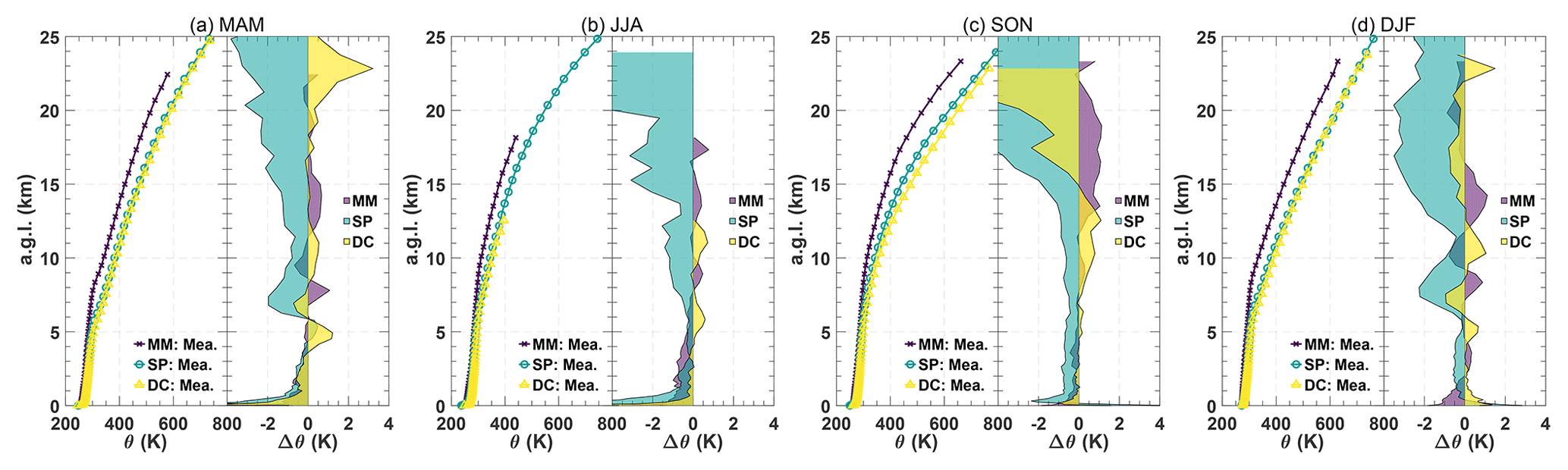
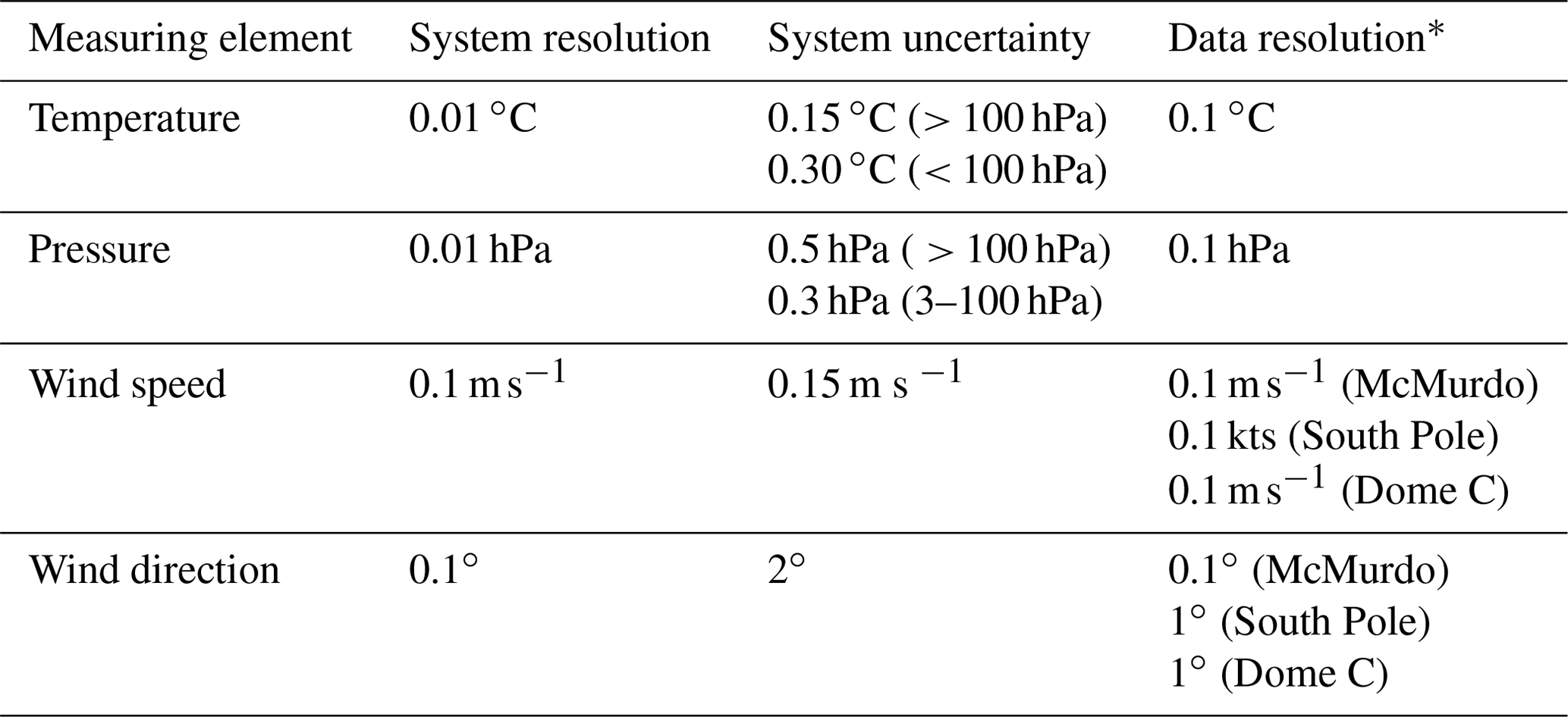
Figure 2 The seasonal median of potential temperature (θ) estimated by the radiosonde measurements (solid lines) and potential temperature difference (Δθ) calculated by the AMPS forecasts minus the radiosonde measurements, i.e., Δθ = θ_AMPS−θ_Mea. (filled areas). Fall: March–May (MAM); winter: June–August (JJA); spring: September–November (SON); summer: December–February (DJF).

Figure 3 As in Fig. 2 but for wind speed V (= $\sqrt{u^{\mathrm{2}}+v^{\mathrm{2}}}$), and ΔV = V_AMPS−V_Mea..

The seasonal median difference of potential temperature (see the filled areas in Fig. 2) and wind speed (see the filled areas in Fig. 3) between radiosoundings and AMPS forecasts are presented. The missing value of the median difference in the upper part of the atmosphere during June–July–August (JJA) indicates that the radiosonde balloon does not reach as high an above-ground level (AGL) in winter as they do in summer, probably because the elastic material of the balloons is more fragile in cold seasons and easier to explode (Hagelin et al., 2008). The lack of measurements may be attributable to some large values of the median difference in the top layer of the profile shown in Figs. 2 and 3, as the AMPS requires the assimilation data from measurements to initialize its numerical model, and the lack of measurements makes it more difficult for the AMPS to simulate atmospheric changes that are close to reality.

Table 2 Statistical evaluations of the potential temperature (θ), wind speed (V), and logarithmic Richardson number (log ₁₀(Ri)) forecasted by the AMPS when compared with the results from radiosonde measurements.

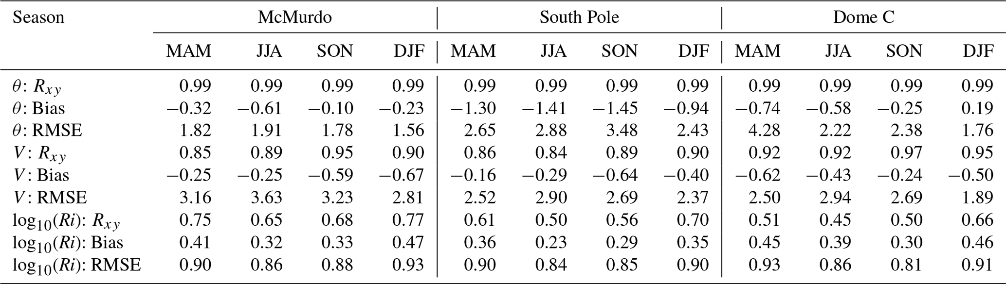
Figure 2 shows that the median difference for θ is of the order of 1 K in the first 5 km, except for atmosphere layer in proximity to the ground. Above 5 km, the AMPS has obviously underestimated the θ at MM, while the forecasts at SP and DC are closer to measurements. Figure 3 shows that the measured wind speed profiles above 10 km at MM and DC are stronger during spring, indicating the occurrence of the Antarctic polar vortex (Boville et al., 1988). However, the change in wind speed above SP is not that obvious, because the Antarctic vortex is roughly pole-centered (Karpetchko et al., 2005). From the filled areas in Fig. 3, the AMPS forecasts appear consistent with the measurements, as the median difference in wind speed is generally ∼ 1 m s⁻¹ and has barely exceeded 2 m s⁻¹, whether the wind is strong or weak. In the first 10 km, most ΔV at the three sites are less than 0, suggesting that the AMPS underestimated the wind speed. Table 2 shows the statistical evaluations of θ and V forecasted by the AMPS. It seems the AMPS can capture the trend of θ and V well since the correlation coefficients (R_xy) are all larger than 0.84.

4.2 Richardson number

4.2.1 Statistical analysis

To evaluate the performance of the AMPS in forecasting the possibility of triggering turbulence over the Antarctic continent, the Ri estimations between radiosoundings and AMPS forecasts will be compared. The calculated value of Ri depends on the vertical resolution of meteorological parameters (Troen and Mahrt, 1986; Holtslag et al., 1990). Thus, the meteorological parameters from the radiosoundings and AMPS forecasts were interpolated into the same height series (as mentioned in Sect. 4.1) to calculate Ri, where $\partial \mathit{\theta }/\partial z$ and ${\left(\partial u/\partial z\right)}^{\mathrm{2}}+{\left(\partial v/\partial z\right)}^{\mathrm{2}}$ for calculating Ri (see Eq. 1) were both computed using a centered finite difference operation, as we found that centered difference performed better than forward difference and backward difference (not shown); i.e., better consistency of Ri between radiosoundings and AMPS forecasts can be achieved using centered difference.

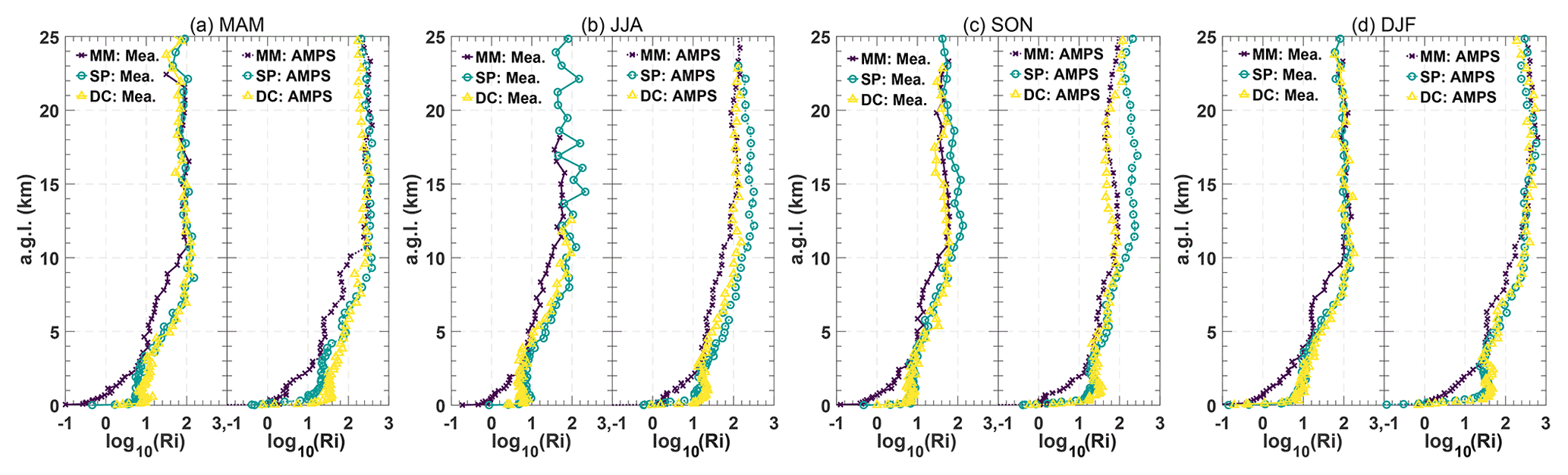
Figure 4 The seasonal median of log ₁₀(Ri) estimated by the AMPS forecasts (solid lines) and the radiosonde measurements (dashed lines).

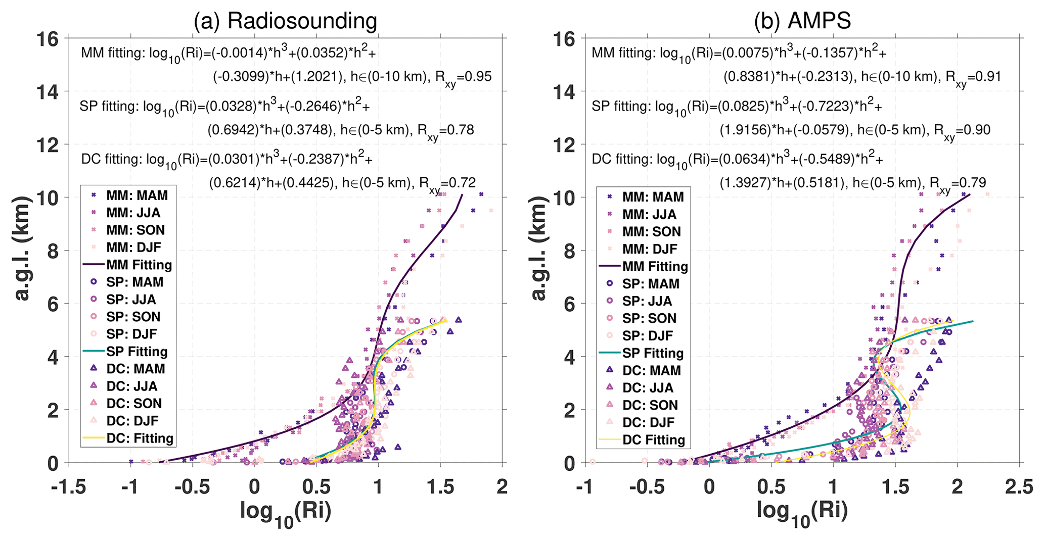
Figure 5 The polynomial curve fitting of near-ground median profiles of log ₁₀(Ri) from Fig. 4. (a) The log ₁₀(Ri) was estimated by the radiosonde measurements. (b) The log ₁₀(Ri) was estimated by the AMPS forecasts.

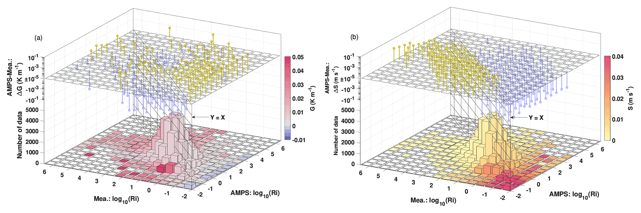
Figure 6 Performance of the AMPS under different atmospheric conditions. Panels (a) and (b) are the case of potential temperature gradient (G = $\partial \mathit{\theta }/\partial z$) and wind shear (S = $\left[\right(\partial u/\partial z{)}^{\mathrm{2}}+(\partial v/\partial z{)}^{\mathrm{2}}{]}^{\mathrm{1}/\mathrm{2}}$), respectively. G (color of the bin in a), S (color of the bin in b), ΔG (stem above the bin in a), and ΔS (stem above the bin in b) are presented using the median value for each 0.5 × 0.5 bin of log ₁₀(Ri).

The seasonal median profiles of log ₁₀(Ri) from radiosoundings and AMPS forecasts are shown in Fig. 4. However, the median differences are not presented like the θ and V. This is because the Ri value can vary massively (by 2 or more orders of magnitude) in the atmosphere, and a precise quantification seems less plausible. Considering this, we initially intended to examine whether the AMPS can reconstruct an accurate shape of log ₁₀(Ri) profile, while median difference is not suitable for this purpose, and the results from radiosoundings and AMPS forecasts are both presented. Nevertheless, the model biases are by all means of great significance, and they will be discussed later (see Table 2 and Fig. 6). In Fig. 4, one can see that the AMPS-forecasted Ri can identify that the atmosphere above MM tends to be more turbulent (Ri is smaller) than SP and DC. In the vertical height direction, the AMPS forecasts can roughly capture the height that can easily trigger turbulence. For example, one can observe that the Ri from radiosoundings and AMPS forecasts both show small values very close to the ground at DC and the SP, which is per the fact that strong atmospheric turbulence is concentrated within the surface layer above the high plateau (Marks et al., 1999; Agabi et al., 2006). A very calm atmosphere (Ri is large) at high altitudes is also consistent with the results given by Travouillon et al. (2003), Aristidi et al. (2005), Trinquet et al. (2008), and Vernin et al. (2009). On the other hand, the AMPS can reconstruct the near-ground log ₁₀(Ri) profiles well in a “convex–concave–convex” (hereafter “C–C–C”) shape, indicated by the radiosonde measurements (see more details in Fig. 5). In terms of time, the AMPS can forecast that the free-atmosphere Ri decreased during spring (SON). This decrease is obvious for MM and DC, where the wind speeds are significantly stronger during SON, as in Fig. 3.

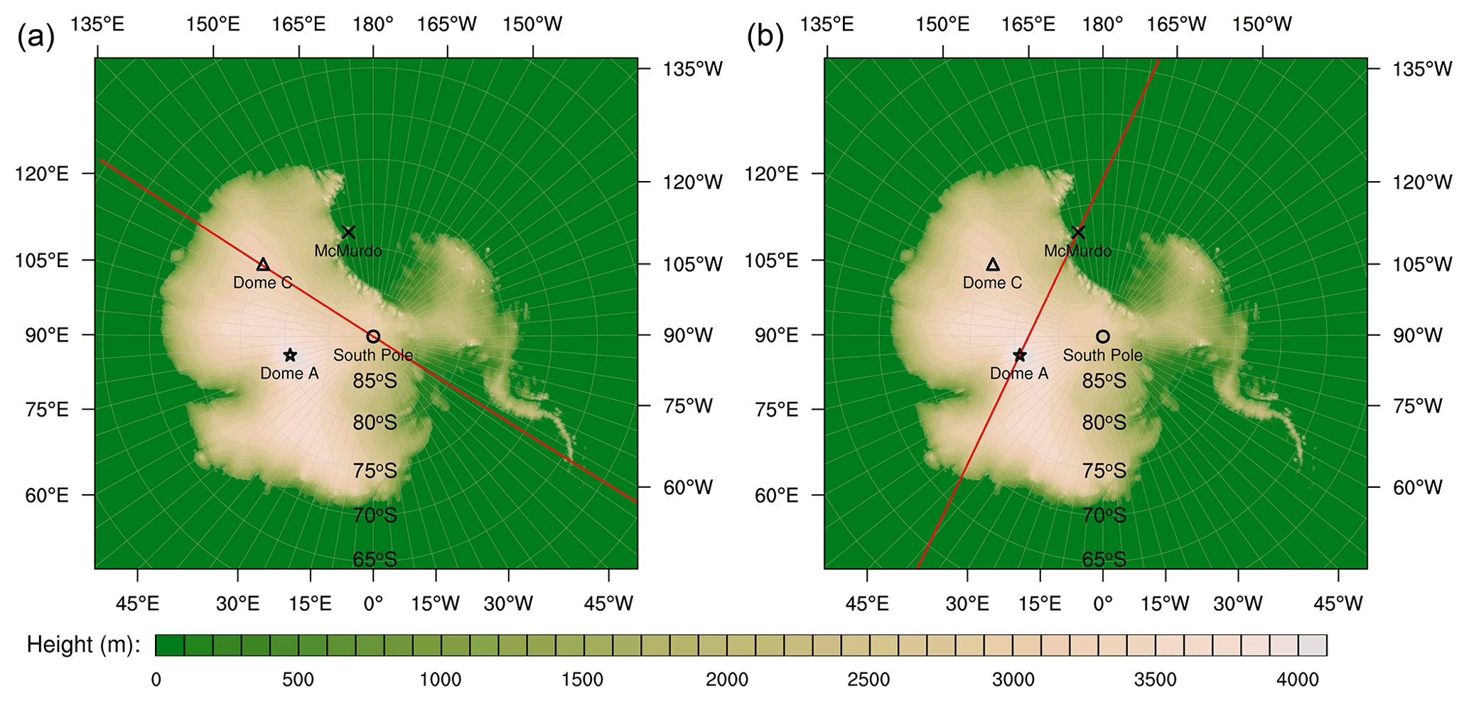
Figure 7 Two lines (marked by red lines) are used to create vertical cross-sections: (a) a line through DC and the SP and (b) a line through DA and MM. The color scale indicates the terrain height (m), where terrain fields are generated from the RAMP2 data set (https://nsidc.org/data/nsidc-0082/versions/2, last access: 1 March 2022).

Quantitative analysis for the estimated Ri from the numerical models was generally missed as it always varies dramatically, e.g., Hagelin et al. (2008), who focused on the qualitative analysis. Nevertheless, quantitative analysis has been tried in this study since that can give a precise evaluation of the forecast ability of the AMPS. Then, the R_xy, mean bias (Bias; AMPS minus radiosonde), and root mean square error (RMSE) are calculated using the combined data of all profiles for each season, where the time difference between radiosoundings and AMPS forecasts was limited to less than 1.5 h. Finally, the seasonal values of the three statistical operators are calculated, as listed in Table 2. However, we want to emphasize that one should focus on the value of R_xy that reflects the tendency, instead of Bias and RMSE, as a precise quantification remains in doubt (Hagelin et al., 2008). The mean values of R_xy for MM, SP, and DC over four seasons are 0.71, 0.59, and 0.53, respectively. The highest R_xy is at MM for DJF (0.77) and the lowest is at DC for JJA (0.45). We found that these two cases correspond to the most unstable and stable atmospheric conditions, with their median values $[{\mathit{\theta }}_{\mathrm{1000}\mathrm{m}}-{\mathit{\theta }}_{\mathrm{0}\mathrm{m}}]/$ [1000–0 m] equal to 0.0038 and 0.0721, respectively. This suggests that the AMPS can better capture the trend of log ₁₀(Ri) at a relatively unstable atmosphere. However, the Bias is the largest (0.47) in the most unstable case. This is because the AMPS overestimated the potential temperature gradient under an unstable atmosphere (see Fig. 6a, which will be discussed later). For the stable atmosphere, the lowest R_xy for log ₁₀(Ri) seems to be consistent with the fact that model errors increase with increasing stability (Nigro et al., 2017).

Table 2 also shows an interesting result: the R_xy of log ₁₀(Ri) is higher when the RMSE of θ and V are smaller. Moreover, Hines et al. (2019) showed that using the Morrison microphysics scheme in the numerical model resulted in a smaller RMSE for temperature and wind than the default scheme (WSM5C) in the AMPS. Therefore, we may conclude that replacing WSM5C with Morrison could improve the AMPS-forecasted log ₁₀(Ri). In other words, using Morrison may lead to a higher R_xy for log ₁₀(Ri), as it simulates dynamic stability with less variability (the RMSE for temperature and wind could be smaller). On the other hand, larger RMSE for θ and V are mainly found during cold months (JJA, SON), indicating that winter dynamic stability is more variable (similar to Bromwich et al., 2013).

Table 2 summarizes that the log ₁₀(Ri) was overestimated by the AMPS at each site for every season (every Bias is positive). This may be due to some local-scale dynamics not being represented properly (see Fig. 6, which will be discussed later). From another perspective, the model results were generally smoother than the measurements, and the atmosphere is less favorable for the occurrence of turbulence under slowly changing meteorological parameters, allowing the AMPS-forecasted Ri to be larger.

The near-ground atmosphere in Antarctica is an important turbulence source, and an analytical function for log ₁₀(Ri) profiles near the ground was fitted to better contextualize the results (as shown in Fig. 5). Figure 5 shows that the near-ground log ₁₀(Ri) profiles are the C–C–C shape. The concave structure in the C–C–C shape could be attributed to the near-ground jet stream (Mihalikova et al., 2012). A cubic polynomial function was used (see the upper part of the plots in Fig. 5) instead of a logarithmic function, because the C–C–C shape seems hard for logarithmic function fitting. Moreover, each fitted curve used the data points of all four seasons in Fig. 4, as the seasonal variation is not too significant. Nevertheless, one can see more details about the temporal variation of log ₁₀(Ri) near the ground in Sect. 4.2.3.

Figure 6 shows the AMPS performance under different potential temperature gradient ($G=\partial \mathit{\theta }/\partial z$) and wind shear ($S=\left[\right(\partial u/\partial z{)}^{\mathrm{2}}+(\partial v/\partial z{)}^{\mathrm{2}}{]}^{\mathrm{1}/\mathrm{2}}$). The statistical results presented in Fig. 6 were counted based on all the collected data points at the three sites (MM, SP, and DC) for an entire year. One can see that the Ri was overestimated by the AMPS at an unstable atmosphere (see light blue bin in Fig. 6a), where the AMPS has overestimated the potential temperature gradient (i.e., ΔG>0). But for strong temperature inversion (see dark red bin in Fig. 6a), the AMPS has underestimated the G and Ri. As for strong wind shear conditions (see dark red bin in Fig. 6b), when the Ri is small (basically corresponding to a near-surface layer with a high probability of triggering strong turbulence, as in Fig. 4), the AMPS has underestimated the intensity of wind shear (ΔS < 0). This may be caused by the AMPS that has underestimated the wind speed near the ground (as in Fig. 3). In sum, if the model aims for a more accurate forecast of Ri, the biases under these atmospheric conditions need to be corrected.

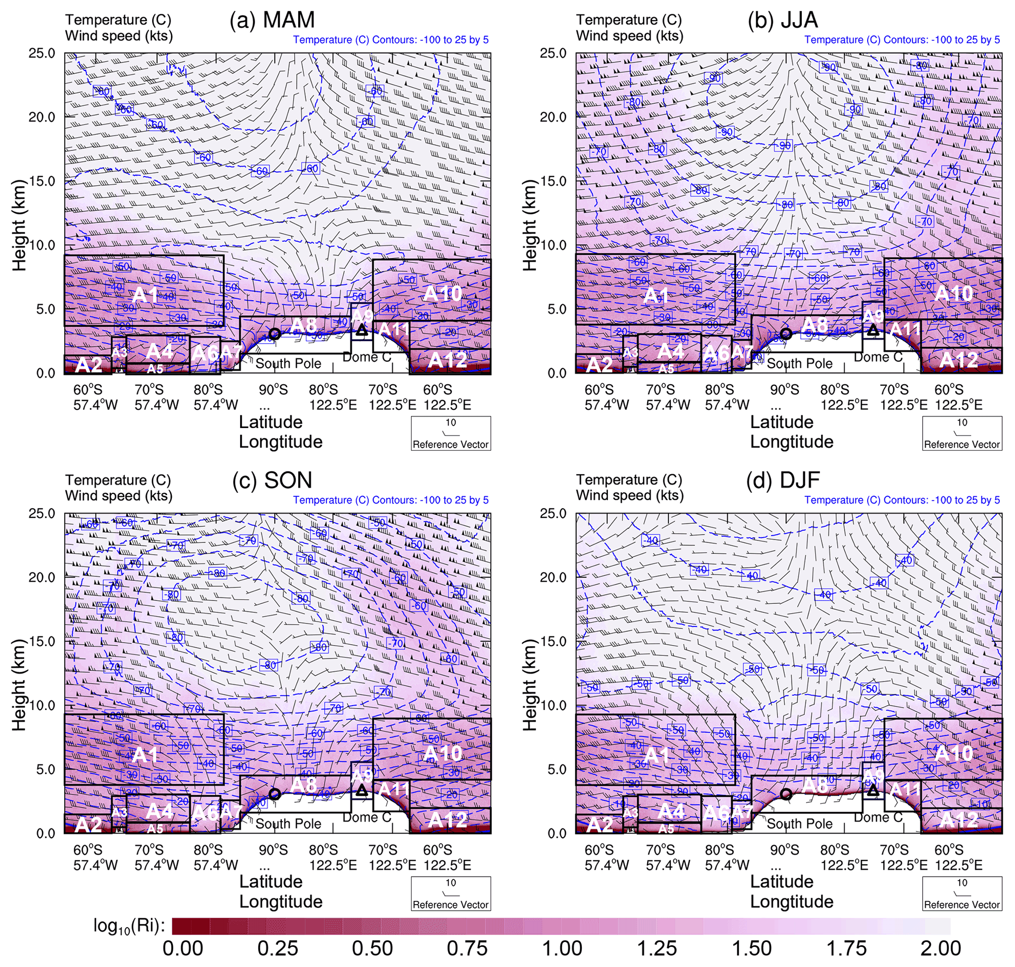
Figure 8 The seasonal median of temperature, wind speed, and log ₁₀(Ri) along the vertical cross-section through the South Pole (black circle) and Dome C (black triangle), as shown by the red line in Fig. 7a. The height (km) on the y axis represents the elevation above sea level. The AX in each plot is used to mark the possible functional areas of some atmospheric activities (as listed in Table 3).

Figure 9 As in Fig. 8 but for the vertical cross-section through Dome A (black star) and McMurdo (black cross), as shown by the red line in Fig. 7b.

4.2.2 Vertical cross-section

The results given in Sect. 4.2.1 show that the AMPS can forecast the main tendency of log ₁₀(Ri). Then, we consider that it is worth a try to use the AMPS-forecasted log ₁₀(Ri) to comprehend the characteristics of atmospheric turbulence in Antarctica. The results of the AMPS-forecasted log ₁₀(Ri) were presented through interpolation of the AMPS grid 2 field at two vertical cross-sections, providing us with a broader perspective on the probability of turbulence triggered in four-dimensional space-time. One vertical cross-section is interpolated through the SP and DC, and another is interpolated through DA and MM, as shown in Fig. 7. The corresponding AMPS forecasts are shown in Figs. 8 and 9, respectively.

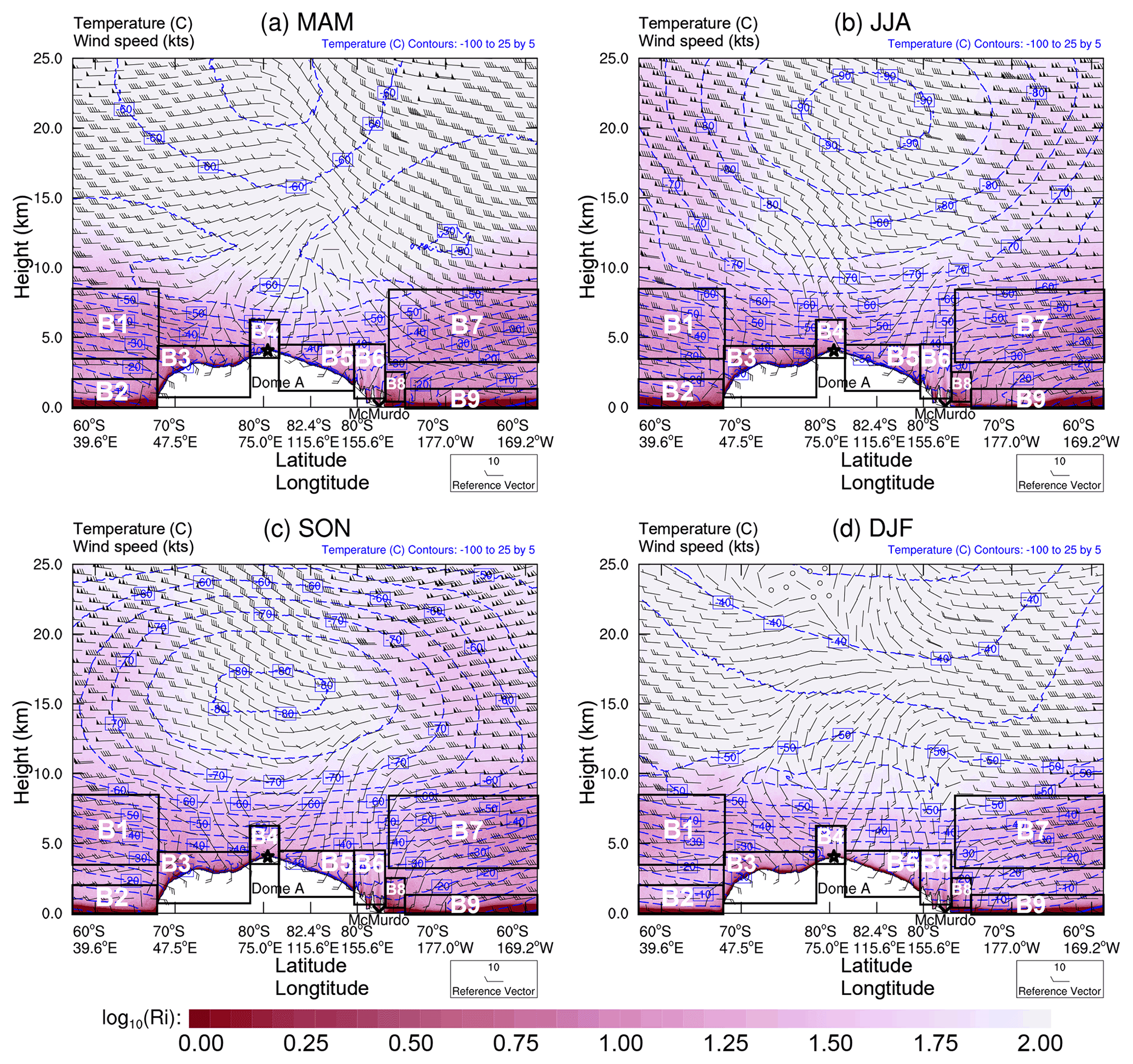
Figures 8 and 9 show the seasonal median values of the AMPS forecasts. The temperature and wind speed were lower above the Antarctic Plateau than over the ocean. In the polar winter (JJA), the temperature contours are dense near the ground above the interior plateau, representing a strong surface-layer temperature inversion (such inversion has been observed by Yagüe et al., 2001; Argentini et al., 2013; Hu et al., 2019). The surface-layer wind speeds increase from the summit to the escarpment region (caused by the well-known katabatic wind over the surface slope area in Antarctica) and then decrease toward the coast, which is consistent with previous measurements (Ma et al., 2010; Rinke et al., 2012). The Ri is obviously larger above the summits (e.g., DA and DC), suggesting that the PBLH could be thin. This agrees with the results from Swain and Gallée (2006), Bonner et al. (2010), and Aristidi et al. (2015).

The results of the Ri distribution from the AMPS outputs provided us with valuable insights into the atmospheric turbulence in the Antarctic region, while using the radiosonde measurements is hard to do so. Here, we attempt to relate the features of atmospheric turbulence to some large-scale phenomena or local-scale dynamics over the Antarctic Plateau and the ocean surrounding it: the shear-induced turbulence (katabatic winds, polar vortices), convection (cloud cooling, boundary layer convection), temperature inversion, and the wave-induced turbulence (orographic gravity waves – OGWs, trapped lee waves – TLWs, inertia-gravity waves – IGWs). Table 3 lists their possible functional areas that are marked in Figs. 8 and 9. This is dedicated to qualitatively evaluating the AMPS outputs and investigating the underlying physical processes of triggering atmospheric turbulence.

As a result of katabatic winds (Rinke et al., 2012), the near-surface wind speeds increase from the interior plateau to the steep slope (Figs. 8 and 9), which is driven by gravity. Strong winds can lead to strong wind shear and increased levels of mechanical turbulence (e.g., Huang et al., 2021; Solanki et al., 2022), as one can see from the surface layer with a small Ri at the escarpment region (see A8 and A11 areas in Fig. 8, B3 and B5 areas in Fig. 9), where the regions between the SP and DC (in A8 area) are also located on the slope (see Fig. 7a) and show a relatively small Ri near the ground.

Table 3 The possible functional areas of some typical large-scale phenomena or local-scale dynamics over the Antarctic Plateau and the ocean surrounding it.

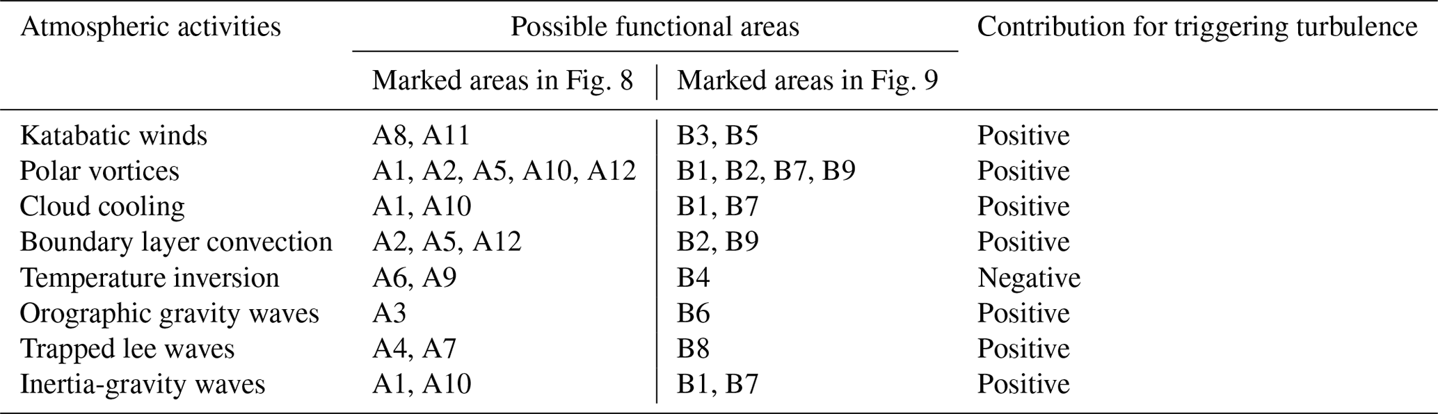
A strong polar vortex implies that the zonal winds are intense, and atmospheric turbulence is more prone to occur. The Antarctic polar vortex reaches its maximum intensity in the winter–spring season (Zuev and Savelieva, 2019a), which corresponds to the relatively turbulent-free atmosphere with low Ri values over the ocean during JJA and SON (see Figs. 8 and 9). Moreover, since the strongest zonal winds are located over the ocean (Zuev and Savelieva, 2019b), the interaction between the zonal wind and the ocean surface may generate wind shear and facilitate the development of turbulence (see areas A2 and A12 in Fig. 8, B2 and B9 in Fig. 9).

Cloud cooling refers to two kinds of cooling-induced turbulence in this study: cloud-top cooling (CTC) and below-cloud-base turbulence (BCT). The CTC is contributed by radiative cooling, which could be one of the driving mechanisms of the mixed-layer turbulence (Deardorff, 1976). The BCT usually occurs below the bases of midlevel clouds accompanied by precipitation that does not reach the ground; cooling by evaporation or sublimation seems to contribute to the turbulence (Kudo, 2013; Kantha et al., 2019). In sum, regions with clouds may advance the development of turbulence. The cloud fraction observed by satellite lidar is higher above the ocean than the Antarctic Plateau (Spinhirne et al., 2005; Saunders et al., 2009). Thus, clouds may benefit small Ri above the ocean (A1 and A10 areas in Fig. 8, plus the B1 and B7 areas in Fig. 9).

Boundary layer convection is generated by forcing from the ground; solar heating of the ground during sunny days causes thermals of warmer air to rise and convection will form (He et al., 2020), then the turbulence could be developed forced by buoyancy (Verma et al., 2017). The albedo of fresh snow over sea ice is very high, while that for open water is relatively small (Hines et al., 2015). Thus, solar heating will be much more prominent over open water and lead to the thermal convection boom. This can be used to reasonably explain the results in Fig. 8, that the Ri over the ocean (A2 area) is smaller than over the ice shelf (A6 area), and the A5 area can be regarded as a “transition region” (sea ice and open water could both exist) between them with an intermediate value of Ri.

The strength of the near-ground temperature inversion forecasted by the AMPS increases from the coast to the high interior, and its strength weakens during polar summer; such a phenomenon has also been observed in previous studies (Hudson and Brandt, 2005; Ma et al., 2010). The general increase in temperature-inversion strength was considered to correspond to a less turbulent atmosphere when the boundary layer is shallower, owing to large stability suppressing turbulence. This corresponds to the larger Ri in the summit area where a stronger temperature inversion occurred (see A9 area in Fig. 8 and B4 area in Fig. 9). A similar phenomenon occurred over the Ronne ice shelf (A6 area in Fig. 8), especially during JJA when the temperature inversion is more obvious. Importantly, it should be noted that it is the range of turbulence (or PBLH) that would be suppressed by the temperature inversion and the turbulence intensity could be strong within the inversion layer (Petenko et al., 2019). For example, the turbulence above Dome C is mainly concentrated in the first tens of meters above the ground (Aristidi et al., 2015).

The development of orographic gravity waves (OGWs) is the interaction between near-surface wind and a mountain barrier (Lv et al., 2021; Zhang et al., 2022a, b). The OGW breaking could be a source of turbulence. Obviously, OGWs can be triggered above the Antarctic Peninsula (A3 area in Fig. 8) and Transantarctic Mountains (B6 area in Fig. 9). But the atmosphere just above the top of the mountain seems to be laminar (e.g., see the larger value of Ri in B6 area). This may be due to the fact that the breaking of the OGWs may not happen immediately after being generated above the mountains.

Trapped lee waves (TLWs) belong to OGWs. Specially, TLWs, as its name implies, tend to form on the lee side of mountains and turbulence may be developed in the downstream (Xue et al., 2022). Thus, the small Ri in the A4 area in Fig. 8 can be attributed to the TLWs forced by the Antarctic Peninsula (see its position in Fig. 7a). It is the same case for the B8 area in Fig. 9 (but forced by the Transantarctic Mountains). The katabatic winds could be linked to TLWs and result in enhanced turbulence. This could explain why the A7 area (Fig. 8) has a small Ri on the lee side of the mountain.

Inertia-gravity waves (IGWs) are influenced by the Coriolis effect (increasing with wind speed), and the frequency of IGWs is close to inertial frequency. The IGWs and Kelvin–Helmholtz instability (which can be characterized by the Ri) are generally presumed to be closely linked. At high latitudes, the IGW energy density's maxima occur at around 5 $\mathrm{km}\mathrm{a}.\mathrm{g}.\mathrm{l}.$ (Zhang et al., 2022b). This may suggest that the IGWs can also contribute to the small Ri above the ocean (A1 and A10 areas in Fig. 8 as well as the B1 and B7 areas in Fig. 9).

In addition, one can see the temporal evolution of Ri vertical cross-sections for a year from the video supplement (vertical cross-section through the red line shown in Fig. 7a: https://doi.org/10.5446/60761, Yang, 2023a and Fig. 7b: https://doi.org/10.5446/60760, Yang, 2023a). It shows that the atmospheric conditions are variable, and a significant transition between laminar flow and turbulent flow could occur at any time. Some activities in Antarctica require a non-turbulent atmosphere, such as astronomical observations (Burton, 2010) and aviation safety (Gultepe and Feltz, 2019). Therefore, real-time forecasting of the Ri is important and helpful, rather than relying solely on the statistical results presented in this study. Furthermore, the video shows that atmospheric turbulence is likely to be triggered over the ocean, moving toward the Antarctic Plateau and weakening. This may be due to the obstruction of the high plateau, which creates a calm atmosphere above it.

4.2.3 Richardson number at the planetary boundary layer height

The Ri is used to determine the PBLH using a critical value (Troen and Mahrt, 1986; Holtslag et al., 1990; Pietroni et al., 2012). Thus, the critical value (or the value of Ri at the PBLH, Ri_PBLH) is worth studying. In addition, previous studies have suggested that the Ri_PBLH depends on the vertical resolution of the data (Troen and Mahrt, 1986; Holtslag et al., 1990). As for the resolution of the AMPS grid, it is necessary to recalculate Ri_PBLH based on the AMPS outputs, since the value of Ri_PBLH is a helpful reference for judging whether atmospheric turbulence is likely to be suppressed (Ri > Ri_PBLH) or developed (Ri < Ri_PBLH).

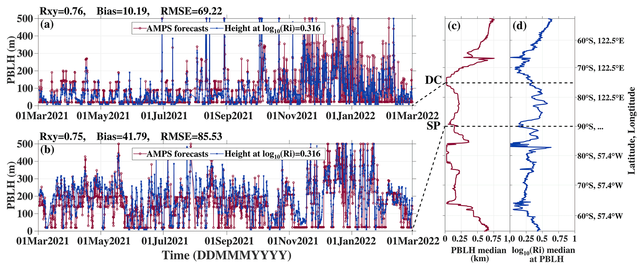
Figure 10 Temporal evolution of PBLH directly forecasted by the AMPS (red circles) and estimated by the height corresponding to log ₁₀(Ri) = 0.316 (blue crosses) at DC (a) and SP (b). Median annual PBLH (c) and log ₁₀(Ri) at the PBLH (d) along the red line through DC and SP shown in Fig.  7a.

Figure 11 As in Fig. 10 but for data above MM and DA as well as the red line through MM and DA shown in Fig. 7b.

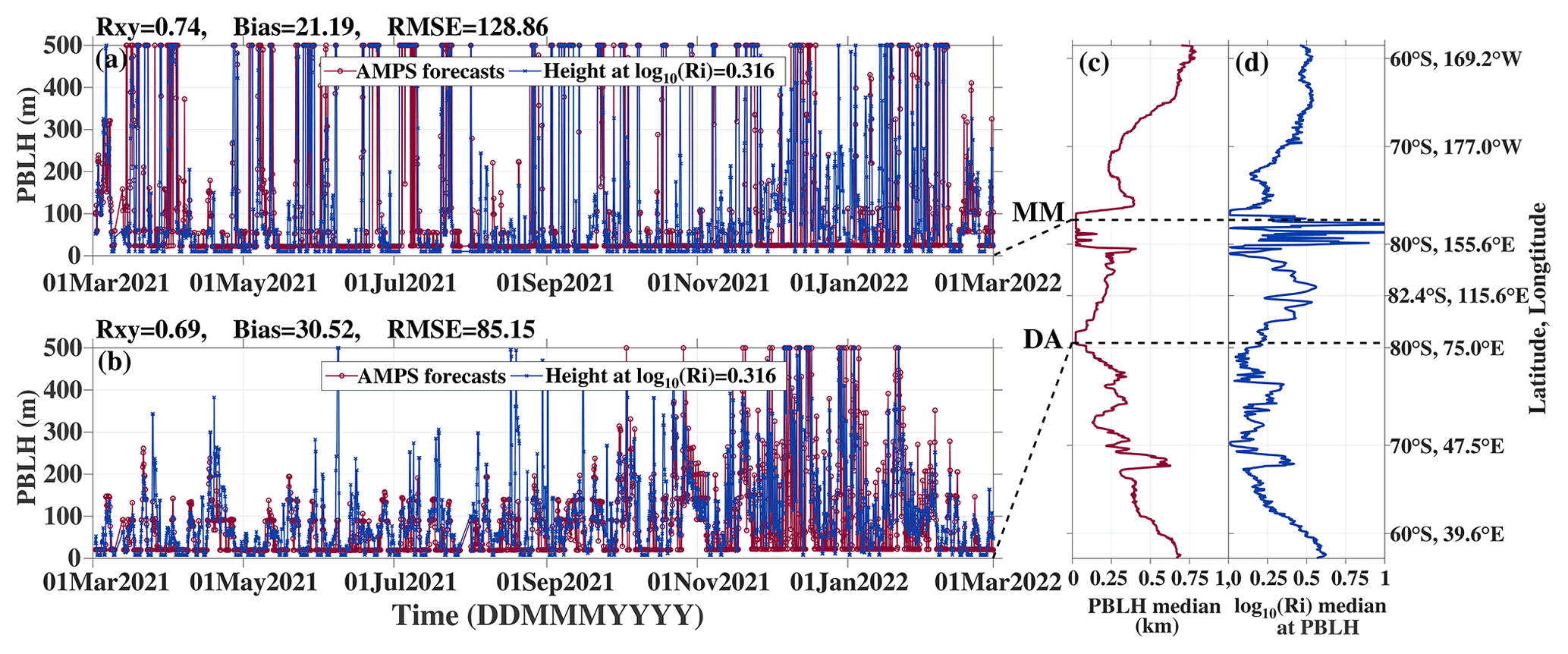
The planetary boundary layer scheme of Polar WRF in the AMPS was the Mellor–Yamada–Janjić (MYJ; Janjić, 1994) scheme, and the ability of the AMPS to model the Antarctic boundary layer has been examined by Wille et al. (2017). The MYJ scheme defines the PBLH, where turbulent kinetic energy decreases to a prescribed value of 0.1 m² s⁻² (Xie et al., 2012). The AMPS forecasts include the values of PBLH. Figures 10a and 11b show that the PBLH directly forecasted by the AMPS was mostly less than 100 m in the summit (DC and DA) during the polar winter, such variation range is consistent with the SODAR observations (DC: Petenko et al., 2014; DA: Bonner et al., 2010); Fig. 10b also displays a result being in accordance with the SODAR observations at the SP, as the measured PBLH was generally within 100–300 m (Travouillon et al., 2003). Thus, the AMPS-forecasted PBLH is considered to be realistic.

Figures 10c and 11c show the median annual PBLH forecasted by AMPS along the red lines in Fig. 7a and b, respectively. A thin PBLH over the plateau can be observed, especially at the Domes (e.g., DA and DC), which is consistent with previous studies (Swain and Gallée, 2006). In contrast, a thick PBLH is shown near the escarpment region, e.g., ∼ 68^∘ S, 122.5^∘ E in Fig. 10c; this corresponds to the relatively low Ri near the ground in the A11 area in Fig. 8.

The log ₁₀(Ri_PBLH) was computed using linear interpolation between the grid with height equal to the AMPS-forecasted PBLH. The median value of log ₁₀(Ri_PBLH) from the combined data of two vertical cross-sections (i.e., Figs. 10d and 11d) was calculated as 0.316, i.e., median value of log ₁₀(Ri_PBLH) equal to 0.316 (or Ri_PBLH=2.07). However, some researchers have employed Ri_PBLH=0.25 when the radiosonde measurements with a higher vertical resolution was used (e.g., at Dome C; Pietroni et al., 2012). Here, the larger Ri_PBLH for the AMPS forecasts may be caused by the coarse vertical grid resolution (as implied from Troen and Mahrt, 1986) and its data smoothness (as mentioned in Sect. 4.2.1; the AMPS forecasts show larger Ri than the radiosoundings, even though they have already been interpolated to the same vertical grid).

To test the credibility of the critical value (i.e., log ₁₀(Ri_PBLH) = 0.316), the PBLH was also derived as the height where the AMPS-forecasted log ₁₀(Ri) decreases to 0.316. The R_xy, Bias, and RMSE of the PBLH between the estimations using the critical value (blue lines in Figs. 10a, b and 11a, b) and the direct forecasts of the AMPS (red lines in Figs. 10a, b and 11a, b) are depicted in the top left of the plot, where Bias indicates the former minus the latter. It appears that the values of R_xy (all larger than 0.69) are almost satisfactory, then we may conclude that log ₁₀(Ri_PBLH) = 0.316 is a reliable critical value for judging the behavior of atmospheric turbulence. The atmosphere layer could be considered turbulent for log ₁₀(Ri_PBLH) < 0.316 and the turbulence intensity could be comparable to that within the boundary layer. However, this critical value may only be valid for using the AMPS forecasts.

5 Conclusions

We have examined the ability of the AMPS to forecast the atmospheric Ri in the Antarctic atmosphere. This includes evaluating the accuracy of meteorological parameters (θ and V, on which the Ri depends), and comparing the log ₁₀(Ri) estimations between radiosoundings and AMPS forecasts. In addition, the analysis of atmospheric log ₁₀(Ri) over the entire Antarctic continent and the ocean surrounding it was presented on an annual timescale. Finally, the log ₁₀(Ri) at the PBLH has been calculated.

From the analysis presented above, we deduce the following.

1. Comparisons of AMPS forecasts with radiosoundings from three representative sites (coast: McMurdo, flank: South Pole, summit: Dome C) show that the forecasts can accurately describe the trend of atmospheric meteorological parameters above the Antarctic continent, as the R_xy for θ reached as high as 0.99 and the R_xy for V are all larger than 0.85 (Table 2).

2. We proved that the AMPS forecasts can identify the main characteristics of atmospheric turbulence over the Antarctic continent in terms of both space and time. The R_xy of log ₁₀(Ri) at MM, SP, and DC are 0.71, 0.59, and 0.53, respectively. And the AMPS can reconstruct the near-ground log ₁₀(Ri) profiles in a “convex–concave–convex” shape indicated by the radiosonde measurements (Fig. 5). We also find that the R_xy of log ₁₀(Ri) would be higher when the RMSE of θ and V are smaller (Table 2). Besides, the AMPS can better capture the trend of log ₁₀(Ri) (R_xy would be larger) at a relatively unstable atmosphere (weaker temperature inversion). Moreover, the values of log ₁₀(Ri) were generally overestimated at the three sites; this is partly the result of the potential temperature gradients at the unstable atmosphere being overestimated by the AMPS, and the AMPS has generally underestimated the wind shear when it was strong.

3. The seasonal medians of the AMPS forecasts from two vertical cross-sections were presented (Figs. 8 and 9), providing us with a broader perspective on when and where atmospheric turbulence could be highly triggered in the Antarctic region. The AMPS-forecasted log ₁₀(Ri) were qualitatively verified, as its statistical distribution behaved as the expected atmospheric properties attributed by some typical large-scale phenomena or local-scale dynamics (katabatic winds, polar vortices, convection, gravity wave, etc.) over the Antarctic Plateau and the ocean surrounding it. For example, a very laminar atmosphere above the Antarctic Plateau and a shallow boundary layer in the Domes area are illustrated by the AMPS forecasts.

4. The log ₁₀(Ri) at the PBLH were calculated and their median value is 0.316, log ₁₀(Ri)=0.316, which in turn was used to calculate PBLH and agree well with the AMPS-forecasted PBLH (R_xy>0.69). The atmospheric layer could be considered turbulent at log ₁₀(Ri)<0.316 and the turbulence intensity could be comparable to that within the boundary layer.

The overall results show that the AMPS can forecast a realistic behavior of Ri, and the turbulence conditions in Antarctica are well revealed; furthermore, some practical operations that want to avoid a turbulent atmosphere – such as astronomical observations (Burton, 2010), aviation safety (Gultepe and Feltz, 2019), and free space optical communication (Yin et al., 2017) – can apply the AMPS-forecasted Ri.