Technical note: Constraining the hydroxyl (OH) radical in the tropics with satellite observations of its drivers – first steps toward assessing the feasibility of a global observation strategy

Despite its importance in controlling the abundance of methane (CH₄) and a myriad of other tropospheric species, the hydroxyl radical (OH) is poorly constrained due to its large spatial heterogeneity and the inability to measure tropospheric OH with satellites. Here, we present a methodology to infer tropospheric column OH (TCOH) in the tropics over the open oceans using a combination of a machine learning model, output from a simulation of the GEOS model, and satellite observations. Our overall goals are to assess the feasibility of our methodology, to identify potential limitations, and to suggest areas of improvement in the current observational network. The methodology reproduces the variability of TCOH from independent 3D model output and of observations from the Atmospheric Tomography mission (ATom). While the methodology also reproduces the magnitude of the 3D model validation set, the accuracy of the magnitude when applied to observations is uncertain because current observations are insufficient to fully evaluate the machine learning model. Despite large uncertainties in some of the satellite retrievals necessary to infer OH, particularly for NO₂ and formaldehyde (HCHO), current satellite observations are of sufficient quality to apply the machine learning methodology, resulting in an error comparable to that of in situ OH observations. Finally, the methodology is not limited to a specific suite of satellite retrievals. Comparison of TCOH determined from two sets of retrievals does show, however, that systematic biases in NO₂, resulting both from retrieval algorithm and instrumental differences, lead to relative biases in the calculated TCOH. Further evaluation of NO₂ retrievals in the remote atmosphere is needed to determine their accuracy. With slight modifications, a similar methodology could likely be expanded to the extratropics and over land, with the benefits of increasing our understanding of the atmospheric oxidation capacity and, for instance, informing understanding of recent CH₄ trends.

1 Introduction

The hydroxyl radical (OH) dictates the lifetime of many tropospheric species, including carbon monoxide (CO), methane (CH₄), and numerous volatile organic compounds (VOCs). Knowledge of OH is therefore necessary to understand the abundance, distribution, and variability of these species. For instance, Rigby et al. (2017) and Laughner et al. (2021) attribute recent trends and increases in CH₄ at least partially to changes in OH abundance. Current constraints on OH are insufficient, however, to assess its relative importance in controlling these trends (Turner et al., 2017).

Differences in OH distributions among chemistry transport models (CTMs) and chemistry climate models (CCMs) suggest that these models are insufficient to inform understanding of OH abundance and variability without further observational constraints. OH abundance can differ by up to 80 % among models constrained with identical emissions in intercomparison projects (Voulgarakis et al., 2013; Nicely et al., 2020; Zhao et al., 2019; Murray et al., 2021), with modeled trends disagreeing with those derived from observationally constrained methods (Stevenson et al., 2020). Variables such as the photolysis frequency of O₃ (JO¹D) (Nicely et al., 2020), the NO_x lifetime (${\mathrm{NO}}_x=\mathrm{NO}+{\mathrm{NO}}_{\mathrm{2}}$), and the oxidation efficiency of VOCs (Murray et al., 2021) contribute to these inter-model variations in OH. Using Gaussian emulation, Wild et al. (2020) found that the relative importance of drivers of OH variability differed widely among three CTMs. Likewise, the response of OH to the El Niño–Southern Oscillation (ENSO), the dominant mode of OH variability on monthly and seasonal timescales (e.g., Anderson et al., 2021; Turner et al., 2018), and other modes of internal climate variability can vary widely among models (Anderson et al., 2021).

Despite this need for better constraints, observations of tropospheric OH are limited. The hydroxyl radical has a lifetime of approximately 1 s (Mao et al., 2009), resulting in large spatial heterogeneity in both the horizontal and vertical. This spatial heterogeneity is further caused by the large variation in the relative importance of drivers of OH loss and production in different regions of the atmosphere (e.g., Spivakovsky et al., 2000; Lelieveld et al., 2016). A strategic, representative in situ observational network is therefore unfeasible. As a result, observations of OH are generally limited to intensive field campaigns (Miller and Brune, 2022) that have narrow spatial and temporal coverage. While remotely sensed OH observations are available, those from satellites are limited to the stratosphere (e.g., Pickett et al., 2008), while ground-based observations of total column OH are dominated by the stratospheric contribution (e.g., Burnett and Minschwaner, 1998).

Reference gases with well-characterized sources and an OH sink, such as methyl chloroform (MCF), can be used to infer OH abundance (Lovelock, 1977). This methodology, however, generally yields no information on spatial heterogeneity beyond the hemispheric scale (e.g., Montzka et al., 2011; Rigby et al., 2017; Naus et al., 2019), although there has been recent success when using three dimensional inversion techniques (Naus et al., 2021). For MCF in particular, recent declines in tropospheric abundance will soon dictate the need for a new reference species (Liang et al., 2017).

Multiple studies have attempted to constrain OH through the creation of proxies and the application of satellite retrievals of OH drivers. Murray et al. (2014) showed that global OH strongly correlated with a combination of JO¹D, water vapor (H₂O_(v)), and the tropospheric sources of reactive nitrogen and carbon in the GEOS-Chem model. Murray et al. (2021) demonstrated that OH correlated with this proxy in multiple CTMs, although the relationship differs strongly among models. Miyazaki et al. (2020) created a data assimilation framework that ingested satellite observations of CO, NO₂, O₃, and HNO₃ (nitric acid) into multiple CTMs. The data assimilation reduced the spread in average OH among the models and brought the interhemispheric ratio closer to unity, in line with values suggested by MCF observations (e.g., Patra et al., 2014). These results demonstrate that the incorporation of satellite observations into a modeling framework can improve the representation of OH. Wolfe et al. (2019) developed a proxy for OH based on formaldehyde (HCHO) production and loss rates. They applied that proxy to satellite HCHO observations to estimate OH columns in the remote troposphere, a region where HCHO abundance is low and the satellite retrievals are reflective of the a priori (Zhu et al., 2016). Using machine learning, chemical transport model output, and retrievals of NO₂ and HCHO, Zhu et al. (2022b) developed a method to estimate surface OH in North American urban areas. Finally, Pimlott et al. (2022) used a steady-state approximation of OH, including primary production from H₂O and O₃ and loss from CO, CH₄, and O₃, to estimate OH between 600 and 700 hPa using observations from IASI (Infrared Atmospheric Sounding Interferometer). A logical next step, building on the results of these studies, is the development of a methodology to constrain OH that ingests multiple satellite retrievals, encompasses the breadth of OH chemical and dynamical drivers, and spans a significant enough portion of the globe to inform variability and trends in CH₄ and CO loss.

Combining machine learning, chemical transport model (CTM) output, and satellite data has the potential to constrain tropospheric column OH (TCOH). A variety of machine learning techniques, such as neural networks (Nicely et al., 2017, 2020; Kelp et al., 2020), self-organizing maps (Stauffer et al., 2016), random forest regression (Keller and Evans, 2019), and gradient boosted regression trees (GBRTs) (Ivatt and Evans, 2020; Zhu et al., 2022b; Anderson et al., 2022), show promise in helping to solve problems in atmospheric chemistry. In particular, Zhu et al. (2022b) and Anderson et al. (2022) demonstrated the ability of GBRTs to predict OH from a chemical transport model with reasonable accuracy. GBRT models (Elith et al., 2008; Chen and Guestrin, 2016) use an ensemble of decision trees to predict the value of a target based on multiple inputs, even for targets with highly non-linear dependencies on the inputs.

Here, we present a methodology to infer clear-sky TCOH in the tropics from space-based observations of its chemical and dynamical drivers with the goal of assessing the feasibility of our methodology, identifying potential limitations, and suggesting areas of improvement in the current observational network. We train a GBRT model using output from a simulation of the NASA GEOS (Goddard Earth Observing System) model and then estimate TCOH in the actual atmosphere at the satellite overpass time using inputs from a suite of satellite retrievals. In Sect. 2, we describe the methodology for generating the machine learning model as well as the satellite retrievals used to constrain TCOH. We then evaluate the suitability of MERRA-2 Global Modeling Initiative (GMI) as a training dataset (Sect. 3) and, in Sect. 4, present a satellite-constrained OH product for 1 month from each season. Finally, in Sect. 5, we explore potential methodological limitations and benefits, including lack of validation data, the impacts of observational uncertainties, and the ability to use different satellites and retrievals as inputs to the GBRT model.

2 Description of the methodology to generate the GBRT model and of the associated datasets

Our overall aim is to demonstrate the feasibility of our approach to constrain TCOH with satellite-based observations over broad regional scales. As a first step, we restrict our analysis to latitudes equatorward of 25^∘ and regions over water. We chose to focus initially on this domain as it has appreciable OH concentrations and simplified chemistry, as compared to regions with large biogenic and anthropogenic VOC emissions. Nevertheless, this portion of the atmosphere accounts for 50 %–60 % of global CO and CH₄ loss. In this section, we describe the creation of the machine learning model used to predict TCOH (Sect. 2.1) for this region as well as the satellite products used as inputs to the machine learning model (Sect. 2.2).

2.1 Creation of the TCOH model

2.1.1 Creation of the GBRT training dataset

For the machine learning model training dataset, we use a subset of output from the MERRA-2 GMI simulation (https://acd-ext.gsfc.nasa.gov/Projects/GEOSCCM/MERRA2GMI/, last access: 31 May 2023). MERRA-2 GMI is a 40-year (1980–2019) simulation of the NASA GEOS model run in replay mode (Orbe et al., 2017) with MERRA-2 (Modern Era Retrospective analysis for Research and Applications, version 2) meteorology (Gelaro et al., 2017). The simulation has a resolution of c180 on the cubed sphere (approximately 0.625^∘ longitude by 0.5^∘ latitude) with 72 vertical layers and uses the GMI chemical mechanism (Duncan et al., 2007; Strahan et al., 2007). Output is available at daily- and monthly-averaged resolution, as well as instantaneous values at 10:00 and 14:00 LST. These times are within approximately 30 min of the overpass times of the satellites described in Sect. 2.2. Anderson et al. (2021) and Strode et al. (2019) provide detailed information about the simulation, including emissions.

The training target for the machine learning model is TCOH. In Anderson et al. (2022), we developed a GBRT parameterization trained on MERRA-2 GMI output to predict in situ OH concentrations using 27 inputs, only a small fraction of which are observable from space. That parameterization, designed to be integrated into the GEOS modeling framework, performed better when there was a separate model for each month as opposed to one model for all months. While that GBRT model is not appropriate for the application described here, we employ a similar approach, creating a separate set of TCOH training targets for each month. We use instantaneous OH output from MERRA-2 GMI at 14:00 local time for each day of a given month across the years 2005 to 2019, a timeframe that maximizes overlap between the operational lifetime of the satellites listed in Table 1 and the period of the MERRA-2 GMI simulation. We omitted data from 2017 to evaluate model performance. For a given month and year, we calculate daily tropospheric column values across the grid, filtering out columns where the maximum cloud fraction in that column was greater than 30 % in order to align the training targets more closely with satellite data, where retrievals of some species are often filtered for cloud cover. This yields approximately 43 000 valid grid boxes per day. For each year, we then average these values to monthly resolution. This results in approximately 600 000 total training targets for each month over the 15-year period.

Table 1 Input variables to the machine learning model and the corresponding satellite retrieval used to create the satellite OH product. Overpass times are ∼ 13:30 LST for all satellites except MOPITT, which has a 10:30 LST overpass.

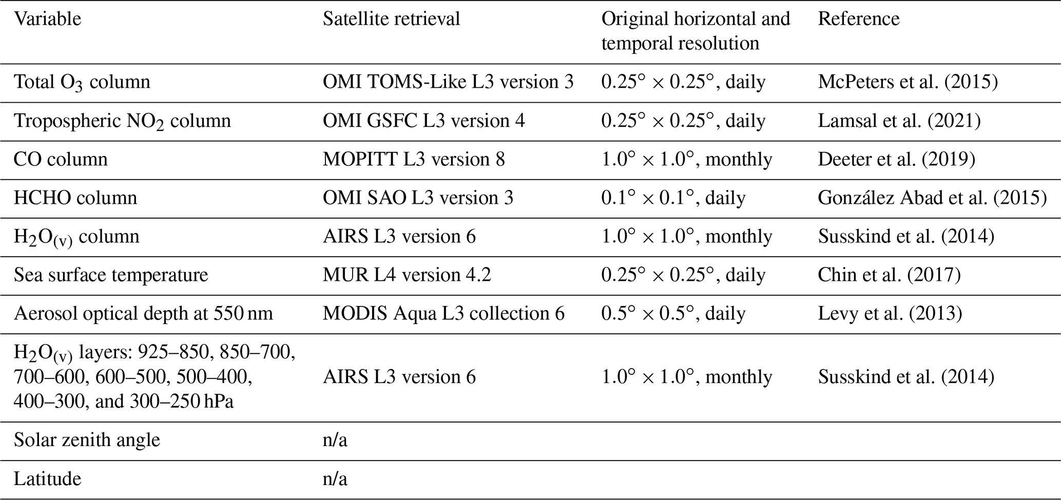
n/a: not applicable.

We selected the input variables for the machine learning model (Table 1) based on their relevance to OH chemistry and variability as well as our current ability to observe the variable with satellites. Performance was similar for a model including total column ozone only and for a model also including the tropospheric column. We therefore use total column ozone because of the uncertainties inherent in separating the column into two parts in the satellite retrieval. We chose the water vapor layers to correspond with the Atmospheric Infrared Sounder (AIRS) layer product. Layers are averages over the indicated pressure range, and we denote the layer names by the highest pressure in that range. We include sea surface temperatures (SSTs) as a proxy for the Indian Ocean Dipole and ENSO, which has a strong impact on OH variability in the tropics (Anderson et al., 2021; Turner et al., 2018; Naus et al., 2021). In addition, we include latitude and solar zenith angle as previous work has shown that these variables can explain a large fraction of the spatial OH variability (Duncan et al., 2000; Anderson et al., 2022).

We sampled the MERRA-2 GMI output to create the training dataset in the same manner as for the TCOH targets. The inputs to the machine learning model each correspond to the same model column as the OH target. All column values are instantaneous and taken from 14:00 LST to correspond with satellite overpass times, except for CO, which is for 10:00 LST, near the Measurement of Pollution in the Troposphere (MOPITT) overpass time. Model performance was similar when using CO output at 14:00 and 10:00 LST, likely because of limited diurnal variability in CO column in the study region. SSTs are monthly averages of 24 h averaged values, and we calculated solar zenith angle at the surface for noon on the 15th of a given month.

2.1.2 Creation and tuning of the GBRT model

We used the XGBoost package (Chen and Guestrin, 2016) version 0.81 in Python version 3.6 to create a GBRT model of TCOH for each month using the training datasets from MERRA-2 GMI. For each month, we used 90 % of the dataset for model training and the remainder for model validation. As mentioned in Sect. 2.1.1, we also used MERRA-2 GMI output from 2017, which was omitted from the training dataset, as further validation.

To maximize parameterization performance while also balancing the potential of overfitting, we tuned hyperparameters, including the learning rate, the maximum tree depth, and the number of trees. We chose hyperparameter values that minimized the parameterization root mean square error (RMSE) of the training dataset. We set the learning rate, which controls the magnitude of change when adding a new tree, to 0.1, while we varied the maximum tree depth and number of trees from 6 to 22 and from 10 to 150, respectively. For both maximum tree depth and number of trees, RMSE initially dropped significantly with increasing value, representing sharp improvement in parameterization performance. RMSE values eventually plateaued, increasing parameterization runtime without noticeably improving performance. A combination of a maximum tree depth of 18 and 100 trees balanced performance with model training and run time.

To determine whether the inputs to the machine learning model improved or hindered performance, we performed a “leave one out” analysis. Using 5-fold cross validation, we retrained the model, individually omitting each of the inputs, to determine the percent difference between the mean RMSE of the 5 folds for the model without a specific input and one including all inputs. Omitting the inputs listed in Table 1 led to increases in the RMSE, suggesting that each is necessary for improved model performance. As a result of this analysis, we do not use water vapor layers for pressures less than 300 hPa because these decreased model performance.

Finally, we found that it was not necessary to apply satellite averaging kernels and shape factors to the training dataset. Of the satellite retrievals used in this work (discussed in Sect. 2.2 and listed in Table 1), only CO, HCHO, and NO₂ could require convolving the model with the averaging kernel. Shape factors for the Ozone Monitoring Instrument (OMI) NO₂ retrieval are determined from a similar setup of the GEOS model, also employing the GMI chemical mechanism and MERRA-2 meteorology. Applying the satellite shape factors to the simulation discussed here would therefore not result in significant changes in the modeled NO₂ (Anderson et al., 2021). To test whether it is necessary to apply the averaging kernels for CO and HCHO, we created a separate training dataset, where we convolved the daily MERRA-2 GMI output with the averaging kernel and a priori from the level 2 data for both species for February 2005–2019. All other inputs were kept the same. We then retrained the model with these adjusted CO and HCHO variables. When we applied the satellite data to the model for February 2017, as described in Sect. 4, the resulting TCOH differed by less than 1 % on average from the model that did not include averaging kernel information. This level of uncertainty is significantly smaller than the other uncertainties discussed in Sect. 5, so we do not include averaging kernels in our analysis.

2.2 Description of satellite products

To create the observationally constrained OH product, we use multiple satellite retrievals, listed in Table  1 and briefly described here. Each instrument is located on board a polar orbiting satellite that provides near-global coverage daily. For each satellite retrieval, we use the level-3 gridded product, with the exception of SST which is level 4. Where necessary, we regridded the retrieval to a common horizontal grid with a resolution of $\mathrm{1.0}{}^{\circ }\times \mathrm{1.0}{}^{\circ }$ and averaged to the monthly scale.

We use these resolutions because, in the study domain, individual pixel retrievals, particularly of NO₂ and HCHO, are frequently at or below detection limits (González Abad et al., 2015; Lamsal et al., 2021), necessitating averaging to relatively coarse temporal and spatial scales. The study domain partially mitigates limitations of the $\mathrm{1.0}{}^{\circ }\times \mathrm{1.0}{}^{\circ }$ resolution, as spatial heterogeneity of the relevant species is generally much lower over the remote tropical oceans than over land. Missing data due to cloud cover and the OMI row anomaly further increase the need for monthly-scale averaging. While other satellites, such as OMPS (Ozone Mapping and Profiler Suite) and TROPOMI (Tropospheric Monitoring Instrument), provide retrievals with increased signal to noise ratios and more complete data coverage, the satellites used here cover a far longer time period. Nevertheless, the $\mathrm{1.0}{}^{\circ }\times \mathrm{1.0}{}^{\circ }$ and monthly resolutions, in combination with the long data record, provide new constraints on regional trends in TCOH and some aspects of TCOH temporal and spatial variability.

We use retrievals of three species – HCHO, O₃, and NO₂ – from OMI, an ultraviolet–visible spectrometer located on board the Aura satellite, which has an overpass of approximately 13:30 local solar time (LST). We use the Smithsonian Astrophysical Observatory (SAO) version-3 HCHO retrieval (González Abad et al., 2015). Wolfe et al. (2019) found that this retrieval captured the variability of the HCHO columns in the remote atmosphere observed during the Atmospheric Tomography (ATom) campaign with little bias. For total column O₃, we use the TOMS-like (Total Ozone Mapping Spectrometer) retrieval version 3 (McPeters et al., 2015), which agrees with ground-based and other satellite observations within approximately 1 % (Labow et al., 2013). Finally, we use the Goddard Space Flight Center version-4 NO₂ tropospheric column retrieval (Lamsal et al., 2021). While previous studies have thoroughly evaluated this retrieval in more polluted atmospheres (e.g., Lamsal et al., 2014; Choi et al., 2020), evaluation in the remote tropical atmosphere, as defined in this study, is limited.

For water vapor and aerosol optical depth (AOD) at 550 nm, we use retrievals from AIRS and the Moderate Resolution Imaging Spectroradiometer (MODIS) instruments, respectively, both located on board the Aqua satellite with an overpass of approximately 13:30 LST. We use the total column water vapor standard physical retrieval as well as the seven water vapor layers listed in Table 1 (Susskind et al., 2014). Multiple studies have evaluated the accuracy of the AIRS H₂O_(v) column and layers retrievals in the remote tropical atmosphere, finding a bias of 5 % or less and high correlation against both remote and in situ observations (Bedka et al., 2010; Anderson et al., 2016; Pérez-Ramírez et al., 2019). We use collection 6 of the dark target MODIS AOD retrieval at 550 nm, which is highly correlated with observations from the AERONET network over the ocean (Levy et al., 2013).

We also use retrievals of CO from MOPITT, which is on board the Terra satellite with an overpass of 10:30 LST. We use the version-8 retrieval that includes both near-infrared and thermal infrared radiances (Deeter et al., 2019). CO retrievals from MOPITT in the remote tropics generally agree with ground-based remotely sensed observations within 10 % (Hedelius et al., 2019; Buchholz et al., 2017).

Finally, we use SSTs from the Multi-scale Ultra-high Resolution (MUR) analysis, which combines nighttime SST observations from multiple satellite platforms, including MODIS, as well as in situ observations and agrees with other SST analyses within 0.36 ^∘C (Chin et al., 2017).

3 Evaluating the suitability of the MERRA-2 GMI simulation as a training dataset

Before generating the GBRT model to predict TCOH, we first demonstrate that the MERRA-2 GMI simulation is suitable to use as a training dataset. Because of the paucity of in situ observations of OH over most of the globe, we necessarily use output from an atmospheric chemistry model to train the machine learning model. The atmospheric chemistry model output must reasonably capture the distribution, magnitude, and ENSO-related variability of OH and the drivers listed in Table 1, as GBRT models are unable to extrapolate beyond the photochemical environments on which they are trained (Anderson et al., 2022).

3.1 Comparison of the distribution and magnitude of simulated OH drivers to observations

Simulated OH from MERRA-2 GMI agrees with observations over the remote ocean within the instrumental uncertainty. Anderson et al. (2021) compared MERRA-2 GMI output to in situ observations from the first two deployments of ATom, finding modest correlation (r² values between 0.3 and 0.78 depending on the hemisphere and season) between observations and the model. The average normalized mean bias was on the order of 20 %, a slight high bias but within the 2σ observational uncertainty of 35 %. Agreement was highest in the remote atmosphere, whereas the largest error was in regions of fresh, continental outflow off the coasts of South America and New Zealand.

The simulation captures both the observed variability and the magnitude of the majority of GBRT model inputs with reasonable fidelity, suggesting that the satellite retrievals highlighted in Sect. 2.2 are suitable inputs for a machine learning model trained on MERRA-2 GMI output (Fig. 1). Figure 1 compares the distribution of the February training dataset created from the MERRA-2 GMI simulation for 2005–2019 to the satellite observations of the indicated species for February 2017, a month omitted from the training dataset. Distributions of the remaining water vapor layers are shown in Fig. S1 in the Supplement. In addition, correlations between observations and MERRA-2 GMI output for February 2017 are shown, as an example, in Figs. S2 and S3. With the exception of HCHO, distributions of the species are similar between the observations and MERRA-2 GMI, with the training dataset encompassing the full range of almost all species. A GBRT model trained on MERRA-2 GMI will therefore likely not have to extrapolate to photochemical environments on which it was not trained when applied to the satellite data. Further, MERRA-2 GMI total column O₃, H₂O_(v) column, AOD, CO, and SSTs are all highly correlated (r² of 0.65 or higher) with their respective satellite observations, and biases are within 10 %, on average. Anderson et al. (2021) did show that MERRA-2 GMI CO columns demonstrate biases of opposite sign in the Northern Hemisphere and Southern Hemisphere, however.

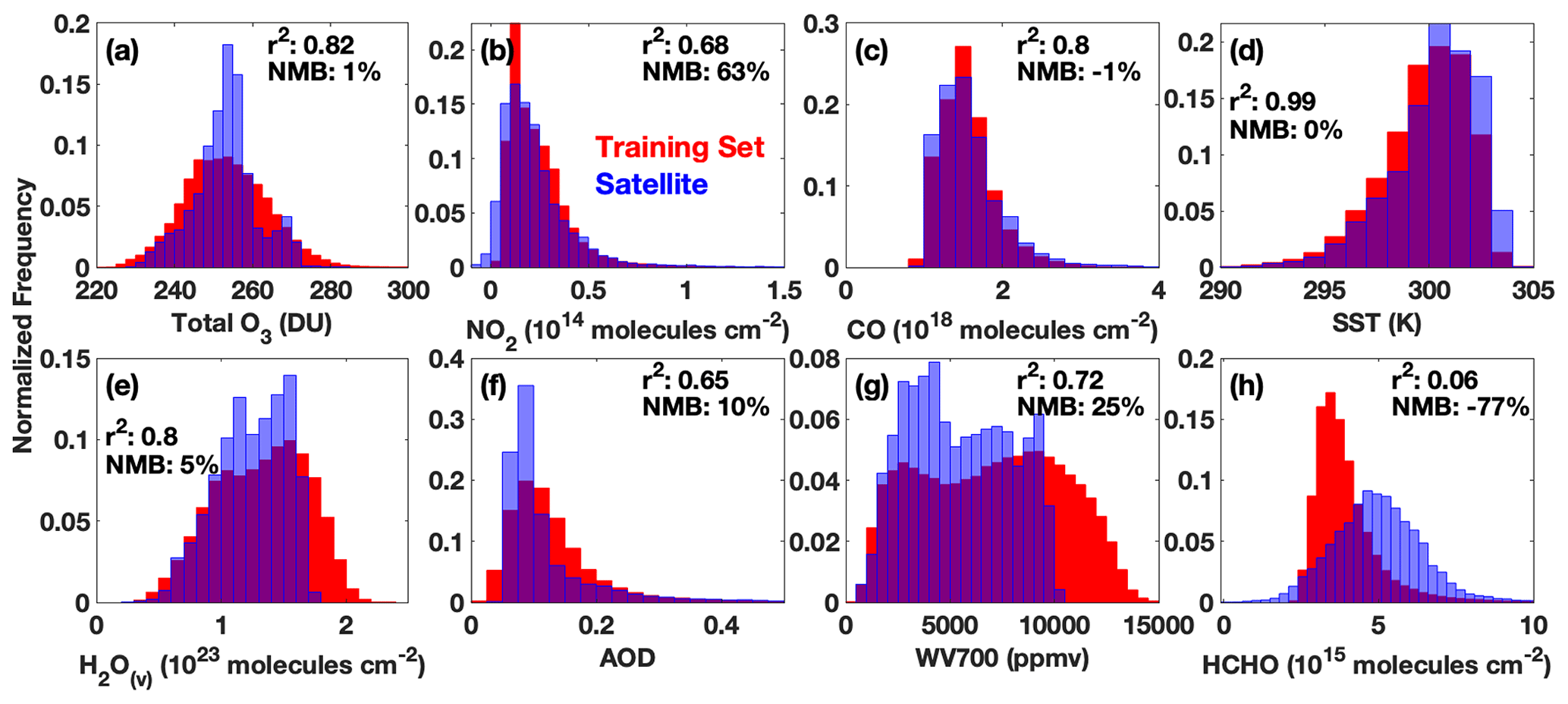
Figure 1 Comparison of the normalized distributions of the training dataset (red) for the February model and satellite observations of the indicated species for February 2017 (blue). Purple indicates regions of overlap. We use H₂O_(v) at 700 hPa as an example for all H₂O_(v) layers. Distributions of the other H₂O_(v) layers are shown in Fig. S1. We also indicate the r² of the correlation between MERRA-2 GMI output for February 2017 and the corresponding satellite retrieval as well as the normalized mean bias of that output.

Agreement between MERRA-2 GMI and satellite observations for NO₂, HCHO, and the H₂O_(v) layers is more variable than for the other species. While modeled NO₂ is moderately correlated with observations (r²=0.68) with relatively similar distributions, MERRA-2 GMI has a normalized mean bias (NMB) of 63 %. This disagreement is most pronounced at low column values, however, where observational uncertainty is large. Further, Anderson et al. (2021) demonstrated distinct regions of bias in NO₂ related to biomass burning and lightning emissions. Modeled HCHO, on the other hand, is not correlated with observations and is biased low by −77 %. Modeled water vapor layers are all modestly correlated with observations (r² of 0.64 or greater) but vary in their bias, with the 925, 850, 700, and 300 hPa layers biased within 30 % and the remaining layers biased up to 71 %.

The satellite product is insensitive to the differences between the HCHO distribution of the satellite and training dataset highlighted in Fig. 1. To determine the effects of the difference in HCHO distribution, we extended the training dataset to cover the full time period of the MERRA-2 GMI simulation (1980–2019) and then subsampled the resultant data to match the satellite HCHO distribution. Extending the training dataset to 1980 allows for the subsampled training dataset to have a similar size (∼600 000 points) as the original training set. We then created a new machine learning model using this sub-sampled dataset and calculated OH fields for February 2017 using the satellite inputs from Table 1. We compared this to the TCOH field calculated from a model using the original training dataset, finding agreement within 5 %. Similarly, the satellite-constrained TCOH product discussed in Sect. 4.2 differs by only 3 % on average from one determined with a GBRT model that excludes HCHO as an input, suggesting the limited impact of potential errors in the MERRA-2 GMI HCHO distribution on model performance. These uncertainties are small in comparison to that resulting from uncertainties in the NO₂ and HCHO satellite retrievals discussed in Sect. 5.2. If the uncertainty of the satellite inputs decreases, as retrievals and instruments improve, then it will become necessary to more closely align the training and observed HCHO distributions.

Finally, because NO₂ and HCHO have the largest differences between satellite observations and the training dataset, we trained a separate machine learning model to predict TCOH, omitting these two species as inputs. When this model was evaluated using the independent MERRA-2 GMI output described in Sect. 4.1, the normalized root mean square error (NRMSE) was 10.1 %, more than a factor of 2 degradation in performance as compared to the baseline model. This suggests that omitting these species from the machine learning model would result in a greater uncertainty in the final TCOH product than that which results from the retrieval uncertainties and the potential discrepancies between observations and the training dataset.

3.2 Evaluation of the simulated ENSO-related variability of OH drivers

Because ENSO is the dominant mode of OH variability (Anderson et al., 2021; Turner et al., 2018), the training dataset must also capture the ENSO-related variability of the GBRT model inputs. Anderson et al. (2021) demonstrated that the correlation of columns of CO, H₂O_(v), and to a lesser extent NO₂, from the MERRA-2 GMI simulation with the Multivariate ENSO Index (MEI) (Wolter and Timlin, 2011) agreed closely with correlations of the corresponding species for observations from MOPITT, AIRS, and OMI. Unsurprisingly, based on the strong correlation and low bias of MERRA-2 GMI SSTs with observations, the simulation also captures the relationship between SSTs and ENSO. The simulation therefore sufficiently captures the ENSO-related variability of these species to act as training data for the GBRT model. We now evaluate this relationship for the remaining GBRT model inputs.

The MERRA-2 GMI-simulated ENSO-related variability of AOD and the various water vapor layers also agrees well with observations. Figures 2 and S4 show the correlation of AOD, HCHO, and the various H₂O_(v) layers with the MEI for the satellite retrievals and MERRA-2 GMI. MERRA-2 GMI captures the general distribution and magnitude of correlation between AOD and ENSO, despite the low optical depths over much of the domain. There are some regional differences, however, particularly in the eastern southern hemispheric Pacific. For the H₂O_(v) layers, the simulation underestimates the magnitude of the correlation in some areas, but in general, there is excellent agreement for all layers throughout the troposphere. This suggests that, despite the high bias discussed above, including the H₂O_(v) layers could provide important, vertically resolved information to the machine learning model.

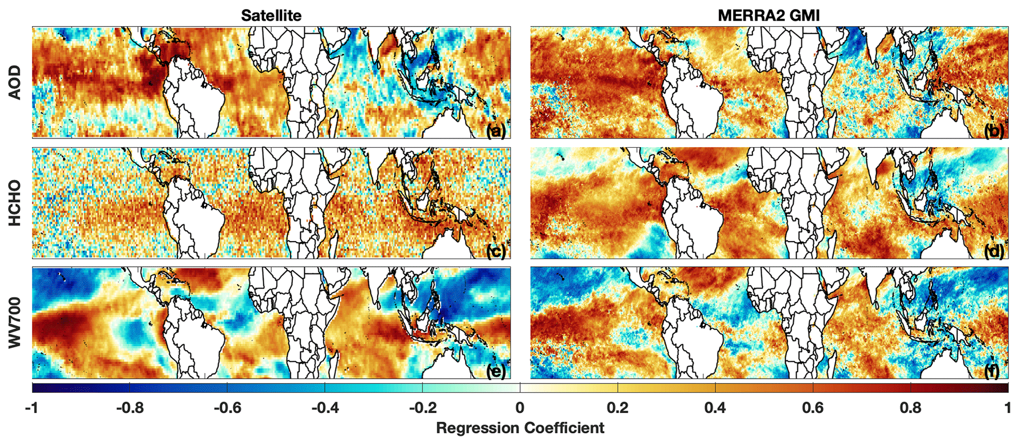
Figure 2 Distribution of the regression coefficient of a linear least squares fit of the indicated variable against the MEI for the respective satellite retrieval (a, c, e) and MERRA-2 GMI (b, d, f) for February. Regressions of AOD are for 2010 to 2019, the years for which we have a 1^∘, gridded satellite product, while HCHO and water vapor 700 hPa are for 2005 to 2019. Satellite data are on a $\mathrm{1}{}^{\circ }\times \mathrm{1}{}^{\circ }$ grid, while model output is at the native model resolution.

Modeled accuracy of the HCHO–ENSO relationship is more difficult to assess. While both the OMI retrieval and MERRA-2 GMI demonstrate broad regions of anti-correlation between HCHO and ENSO, the correlations with OMI HCHO are weaker and noisier than for the other satellite retrievals. Over much of the domain, HCHO abundance is low, often at or below the retrieval detection limit, suggesting that the HCHO retrieval might not be of sufficient quality to capture ENSO-related variability. We investigate the impacts of the HCHO observational uncertainty in Sect. 5.

Finally, because we use total column O₃ as an input to the GBRT model, we do not evaluate the relationship between ENSO and O₃, as the stratosphere dominates the O₃ column and the ENSO-related variability is mostly confined to the troposphere. Oman et al. (2013) found that a GEOS CCM simulation and a combination of O₃ retrievals from the Microwave Limb Sounder (MLS) and the Tropospheric Emission Spectrometer (TES) exhibited similar ENSO-related variability in the middle and upper troposphere, demonstrating that simulations in the GEOS framework can capture this relationship. If a TES-like satellite retrieval were currently available, it could be a valuable contributor to the GBRT model described here, as it would provide vertically resolved information about one of the primary drivers of OH production.

4 Tropical tropospheric column OH constrained with observations of its drivers

We now demonstrate the ability of the GBRT model to determine TCOH. First, we show that the GBRT model can reproduce MERRA-2 GMI modeled TCOH from a year independent of the training dataset, a so-called “hold out set” (Sect. 4.1). We then input satellite data from 1 month from each season into the GBRT model to evaluate the realism of the calculated TCOH fields (Sect. 4.2).

4.1 Evaluation with an independent year from MERRA-2 GMI

The machine learning model is able to capture both the magnitude and the variability of TCOH across each season when applied to MERRA-2 GMI output from 2017, a year independent of the training dataset. For August 2017 (Fig. 3b), the predicted TCOH is highly correlated with MERRA-2 GMI (r² of 0.98). TCOH from the machine learning model agrees with the CTM simulation within 4.8 % on average. The overall NMB is negligible (−0.1 %), although there are some regions of coherent bias (Fig. 3a). Results are similar for February, May, and October 2017 (Fig. S5). The normalized root mean square error for each of these months is comparable to that found for a GBRT parameterization of OH created with a similar methodology that included 27 inputs (Anderson et al., 2022). This suggests that limiting inputs to model variables observable from space does not degrade the ability of the machine learning model to predict TCOH. The low bias and high correlation between the GBRT and MERRA-2 GMI TCOH for all 4 months examined here also suggests that any potential overfitting by the GBRT model is minimal.

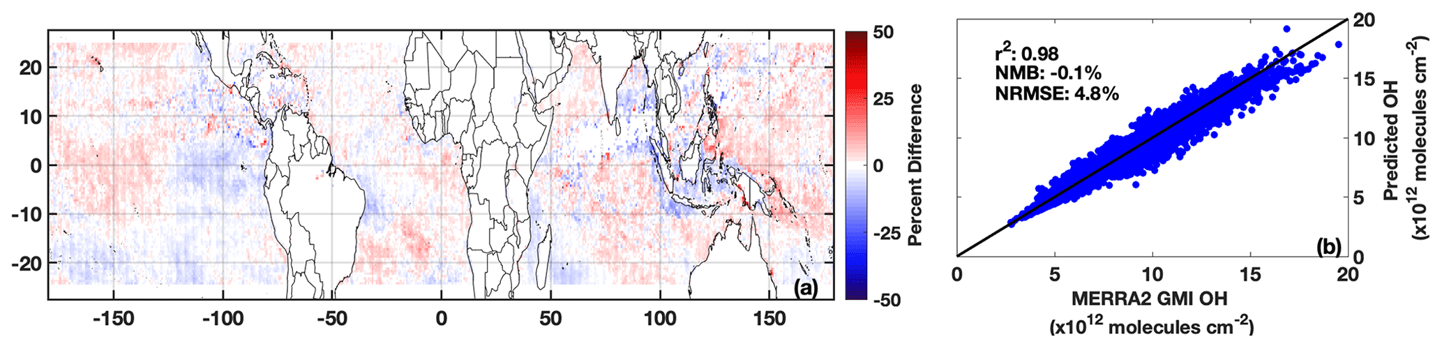
Figure 3 Percent difference between TCOH predicted by the machine learning model and that from MERRA-2 GMI for August 2017, a month and year omitted from the training dataset (a). A regression of the machine learning TCOH against MERRA-2 GMI for the same month (b). The r² of a linear, least squares regression, the normalized mean bias (NMB), and normalized root mean square error (NRMSE) are also indicated.

4.2 TCOH from satellite observations of its drivers

We now apply satellite data from the 4 months corresponding to the ATom campaign (August 2016, February 2017, October 2017, and May 2018) to the GBRT model to determine TCOH fields across the tropics. More details about ATom as well as evaluation of the GBRT model with ATom observations are in Sect. 5. We use the satellite observations listed in Table 1, all of which have been averaged to the monthly scale and to a $\mathrm{1}{}^{\circ }\times \mathrm{1}{}^{\circ }$ horizontal resolution. We include only grid boxes with observations for all GBRT model inputs and where those observations are within the range of the corresponding inputs from the training dataset. Because the satellite inputs for most species exclude grid boxes with a cloud fraction greater than approximately 30 %, the product presented here represents predominantly clear sky conditions.

The GBRT model and multi-satellite inputs yield TCOH fields that are geophysically credible based on our current understanding of OH photochemistry. Although the domain-wide average changes little with season, with a minimum of 5.84×10¹² molec. cm⁻² in May 2018 and a maximum of 6.35×10¹² molec. cm⁻² in August 2016, the spatial distribution varies widely among the 4 months (Fig. 4). In both February 2017 and August 2016, TCOH minimizes in the winter hemisphere, consistent with lower OH production due to low insolation. The reverse is true for the summer hemisphere. In addition, TCOH maximizes in regions with strong continental outflow and along coastlines, regions likely to be impacted by anthropogenic and biomass burning emissions of OH drivers.

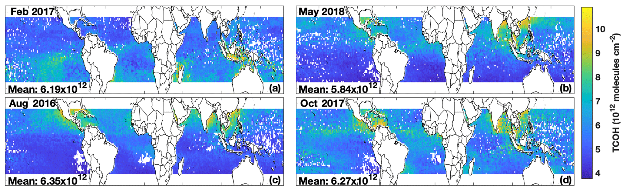
Figure 4 TCOH calculated with the machine learning model using satellite inputs for the months of each ATom deployment: February 2017 (a), May 2018 (b), August 2016 (c), and October 2017 (d). The mean, domain-wide TCOH value in molec. cm⁻² for each month is also indicated.

In general, TCOH from the multi-satellite product differs in both magnitude and distribution from the MERRA-2 GMI simulation. For example, for February 2017, mean MERRA-2 GMI TCOH is 6.96×10¹² molec. cm⁻², 12 % higher than the satellite product (Fig. S6). This is consistent with the comparison to in situ observations discussed in Sect. 3.1 where MERRA-2 GMI overestimates ATom observations by ∼20 % and underestimates CH₄ lifetime, suggesting that the satellite product is again of reasonable magnitude. While understanding the satellite–model differences in TCOH is beyond the scope of this work, we consider the variety in TCOH spatial distributions generated by the GBRT model to be promising. The difference between the satellite-constrained product and MERRA-2 GMI lends some confidence that the GBRT model is not overfit or “tied” to geographic determiners in the training dataset, but rather it is sensitive to variations in the chemical and dynamical drivers of OH. These results all suggest that the methodology presented here can produce a reasonable satellite TCOH product in the tropics, with values and distributions independent of the chemistry model used to create the GBRT model.

5 Understanding and mitigating potential challenges in using this methodology to constrain TCOH

In this section, we outline possible limitations of the machine learning methodology and the current observational network of the GBRT model inputs and provide potential means to mitigate these limitations where necessary. In Sect. 5.1, we discuss the current lack of sufficient in situ observations to thoroughly evaluate the methodology, highlighting this point by validating the GBRT model with data from the ATom campaign. In Sect. 5.2, we investigate the impacts of random retrieval errors in satellite retrievals on the TCOH product, while in Sect. 5.3, we evaluate the impacts on TCOH when using different satellite retrievals as inputs.

5.1 Insufficient in situ observations for thorough independent evaluation

While we demonstrated in Sect. 4.1 that TCOH calculated with the GBRT model agrees closely with a hold-out set from MERRA-2 GMI, it is also important to demonstrate that the GBRT model can replicate observed TCOH from the actual atmosphere. Because the satellite TCOH product shown in Fig. 4 is monthly and at a $\mathrm{1}{}^{\circ }\times \mathrm{1}{}^{\circ }$ resolution, however, there are no observations with which to evaluate the product. We can test the ability of the GBRT model to reproduce observed TCOH from field campaigns, however, assuming there are concomitant observations of the input species listed in Table 1. The additional need for tropospheric column values of many of these species severely limits the datasets available for validation. To our knowledge, the ATom campaign is the only source of the required inputs with enough observations to attempt a limited validation.

During ATom (Thompson et al., 2022), scientists measured a suite of air quality and climate relevant trace gases and aerosols throughout the atmosphere above the remote Pacific and Atlantic. ATom took place in four parts: ATom 1 (July–August 2016), ATom 2 (January–February 2017), ATom 3 (September–October 2017), and ATom 4 (April–May 2018). During each deployment, flights consisted of a series of ascents and descents across all tropical latitudes over the Pacific and Atlantic oceans. This allows for the calculation of tropospheric column content of the observed species and evaluation of the machine learning model across most latitudes of our study domain and across all seasons.

To evaluate the GBRT model performance, we calculated TCOH using a modified GBRT model and observations from the ATom deployments as inputs. We then compared the values to the observed OH columns. To calculate the column values from the observations, we averaged data into 25 hPa pressure bins for each ATom profile. We filled in missing data using a log-linear interpolation and then integrated the column. Our analysis here includes only profiles with observations of all necessary species, which spanned at least 700 hPa, and where less than 25 % of the pressure bin values were interpolated. We also omitted any profiles that had pressure bins with negative OH values. In addition, we restrict our analysis to latitudes within 25^∘ of the Equator and profiles conducted between 12:00 and 15:00 LST. Values for total column O₃, AOD, and SSTs, for which there were no observations during ATom, were taken from the MERRA-2 GMI simulation from the grid box closest to the center of the respective profile. Because ATom profiles did not span the entire tropospheric column, we trained a separate GBRT model where OH and all tropospheric column input variables were substituted with columns spanning 990–250 hPa, the median range of ATom profiles. This allows for a more direct comparison between observed and modeled TCOH. The spatial distribution of the valid ATom columns and the corresponding columns calculated with the GBRT model are shown in Fig. S7.

The GBRT model captures the variability of the observed TCOH, and, while there is a modest overall high bias, the median normalized absolute error of 28.3 % is within observational uncertainty. When applied to all ATom deployments, predicted TCOH is correlated with the observations with an r² of 0.67 and a mean bias of 1.14×10¹² molec. cm⁻² (Fig. 5). Many of the data points agree within the combined modeled and observational uncertainty. The r² values for individual deployments are 0.88 for ATom 1, 0.73 for ATom 2, and 0.78 for ATom 3 and 4. The level of agreement between observed and predicted OH is comparable or better than that of other methods to infer OH from space. For example, Pimlott et al. (2022) found an r of 0.78 (r²=0.61) when estimating ATom OH using a steady-state approach, with r values ranging from 0.51 to 0.85 (r² of 0.26 to 0.72) for the different deployments. The level of agreement we show here therefore demonstrates the validity of the machine learning method to capture the variability of OH.

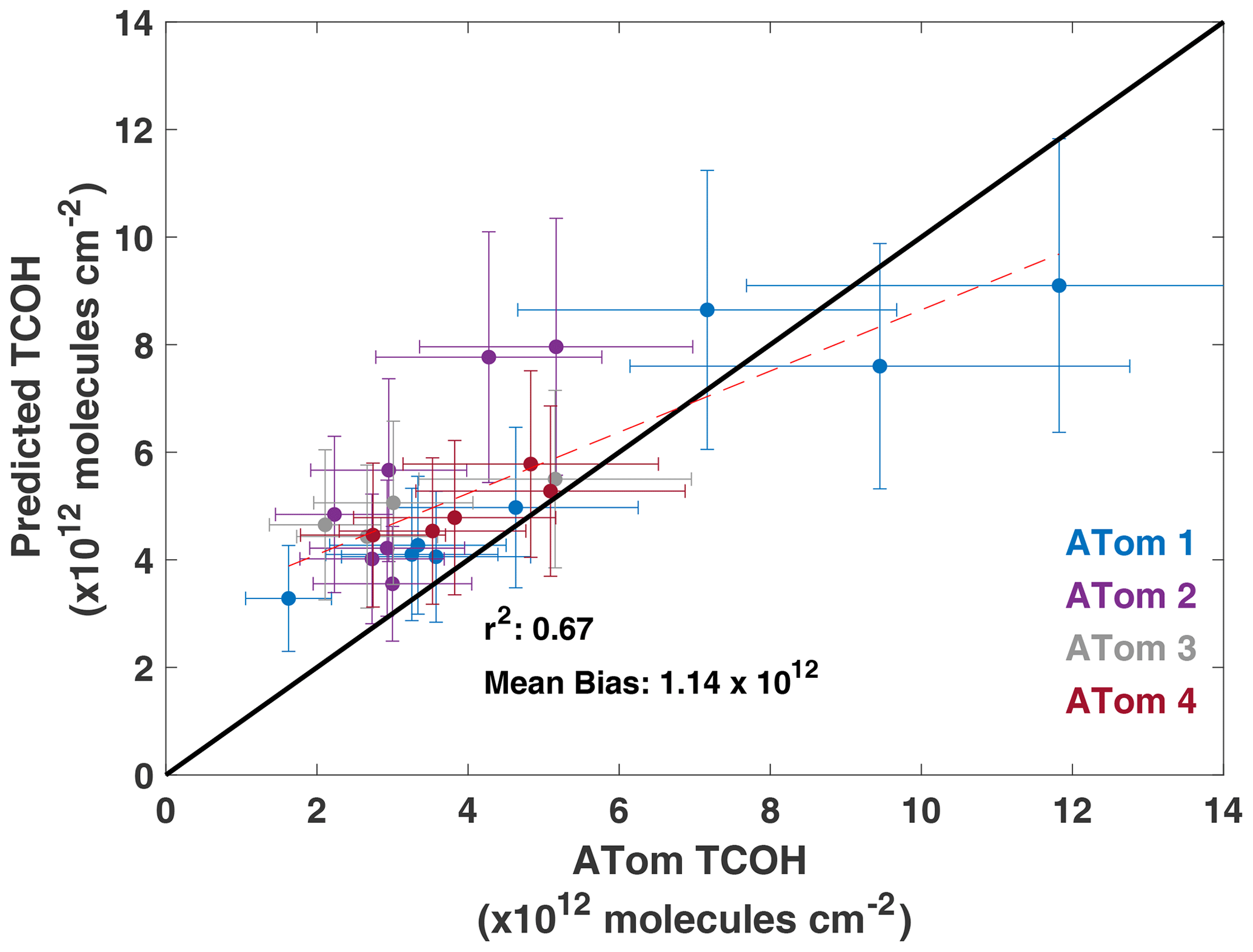
Figure 5 Regression of TCOH observed from the ATom deployments against that predicted from the GBRT model. Error bars represent the 2σ observational uncertainty as reported in Brune et al. (2020) and the GBRT uncertainty described in Sect. 5.2. The r² of a linear least squares fit and the mean bias are also shown.

The source of the model–measurement disagreement, with over- and underprediction at low and high column content respectively, is unclear, although there are multiple potential error sources. For example, a typical profile taken during ATom spanned 300–400 km in latitude, disconnecting the top and bottom of the profile in space. This is in contrast to the data used to train the model, which were vertical columns over one location. This could lead to a degradation in model performance when applied to ATom, since the columns are not directly analogous to the training dataset. These effects are likely limited because ATom observations are in the remote atmosphere, where the spatial distribution of relevant species is likely to be more homogeneous than over land.

Further, there is a known interference with the ATom NO₂ observations, suggesting another possible contributor to disagreement between measured and modeled OH. Because of thermal degradation of NO₂ reservoir species, such as organic nitrates and peroxyacetyl nitrate, in the instrument inlet, ATom NO₂ observations are likely biased high (Silvern et al., 2018; Shah et al., 2023; Nault et al., 2015). To test the potential impact of NO₂ on the predicted OH columns, we applied the ATom observations to a model that omits NO₂ as an input. Removing NO₂ increases the r² to 0.74, decreases the mean bias to 0.82×10¹² molec. cm⁻², and decreases the median normalized absolute error slightly to 25.7 % (Fig. S8). These improvements in performance suggest that errors in NO₂ could be contributing to the measurement–model differences. Omitting NO₂ does, however, likely introduce additional errors as NO_x compounds are essential to OH production in some regions of the atmosphere. When we apply the hold-out set from MERRA-2 GMI to this model, for example, the NRMSE increases by approximately 50 %, highlighting the importance of keeping NO₂ as an input variable.

For more certain evaluation of the GBRT model with observations, greater certainty in the in situ NO₂ observations is needed. Although the in situ observations are insufficient to evaluate the absolute accuracy of the product, the results presented here demonstrate that a machine learning model trained on data from a CTM simulation can capture TCOH variability in the actual atmosphere and suggest that predicted OH columns agree with observations within instrumental uncertainty.

5.2 Impacts of uncertainties in the satellite retrievals on TCOH

In the remote atmosphere where HCHO and NO₂ abundances are low, retrieval uncertainty of an individual pixel for both species can be on the order of 100 % and is often reflective of the a priori (González Abad et al., 2015; Lamsal et al., 2021). Given the importance of these species to the GBRT model as well as to OH chemistry, it is necessary to determine how the propagation of the retrieval uncertainties from these and other model inputs impacts the predicted TCOH.

We determined the total uncertainty in TCOH from all inputs as well as the resultant uncertainty from each individual input for February 2017. First, we estimated an average retrieval uncertainty for each input based on reported values in the retrieval files or from the literature (Table S1 in the Supplement). We note that for NO₂ and HCHO we use a fit uncertainty for a single retrieval. Because we are using monthly averaged data at $\mathrm{1}{}^{\circ }\times \mathrm{1}{}^{\circ }$ horizontal resolution, this likely significantly overestimates the actual uncertainty in these retrievals as the random error from individual pixels will tend to cancel when averaged over such large spatial and temporal scales. Our results are therefore an upper bound on the estimated TCOH uncertainty.

Next, for each grid box and model input, we created a Gaussian distribution of 2000 values with the modeled value for February 2017 as the mean and the estimated uncertainty as the standard deviation. For each input, we then ran the GBRT model 2000 times to create a distribution of predicted TCOH values for each grid box. The normalized uncertainty in TCOH attributable to a given input is the ratio of the standard deviation of the resultant distribution divided by the mean value. We repeated this process individually for all inputs. In addition, to estimate a total uncertainty in TCOH, we varied all inputs simultaneously with the same Gaussian distributions described above.

Uncertainty from the NO₂ retrieval, and to a lesser extent HCHO, dominates the total uncertainty in the TCOH product but is of a magnitude comparable to that of in situ OH observations. Median TCOH 1σ uncertainty resulting from NO₂ is 16.5 %, with maxima in the remote atmosphere in regions where NO₂ columns are low. Median uncertainty in TCOH resulting from HCHO is 7 %, averaged over the study domain, despite the large uncertainty in the HCHO retrieval itself. In contrast to NO₂, uncertainties in TCOH resulting from HCHO maximize in regions with higher HCHO columns (Fig. 6). The magnitude of that uncertainty is likely an overestimate as the actual retrieval uncertainty for HCHO in these regions is significantly lower than the value assumed for the error analysis. In comparison, median TCOH uncertainties resulting from other inputs are 2.9 % or less (Figs. S9 and S10). Total TCOH uncertainty is 16.6 % and is dominated by the NO₂ uncertainty. This uncertainty analysis is in general agreement with the model feature importance (Fig. S11), a measure of the relative importance of GBRT model inputs, where HCHO and NO₂ consistently have the largest values of the satellite inputs.

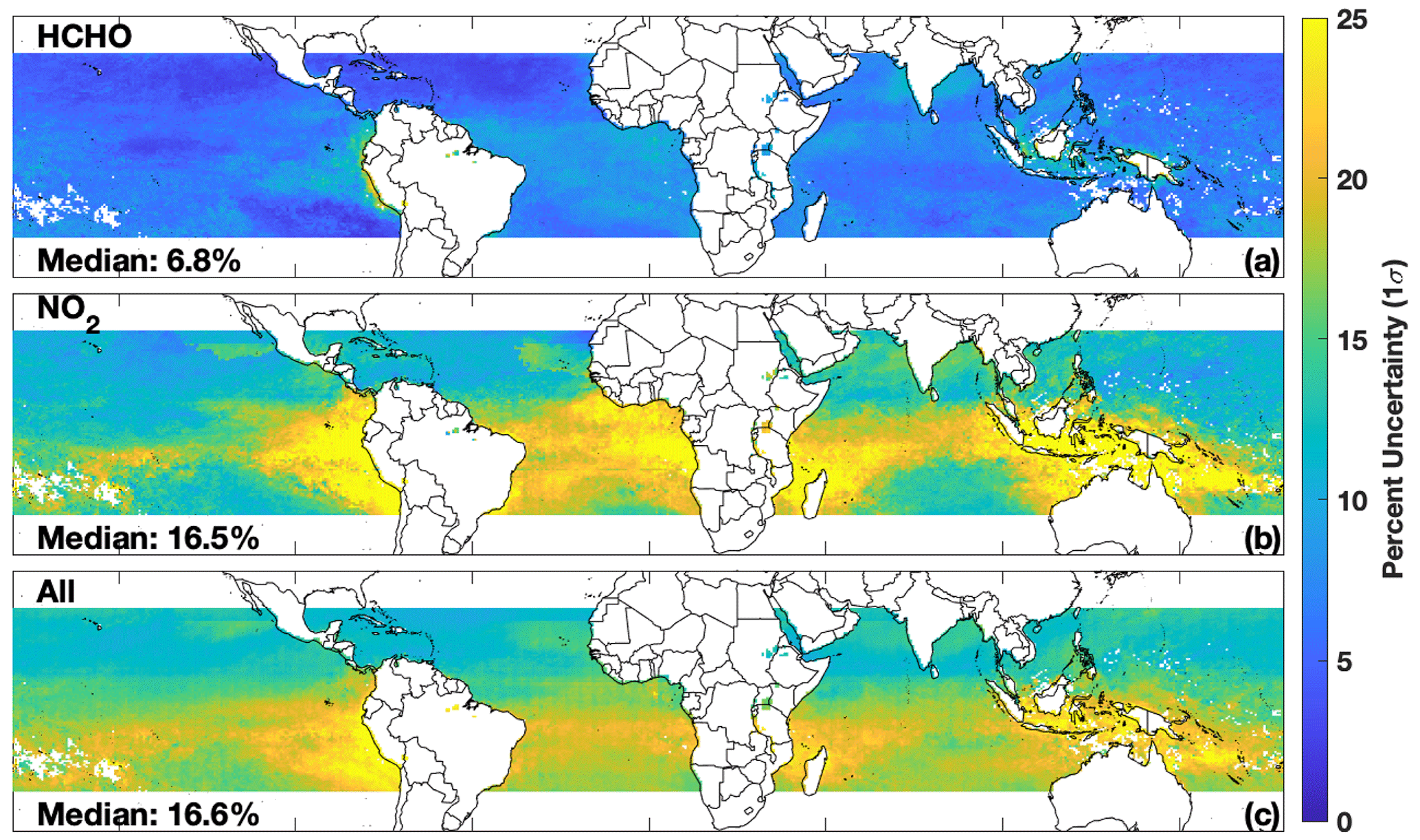
Figure 6 Normalized 1σ uncertainty in the satellite TCOH product due to uncertainties in the HCHO (a) and NO₂ (b) retrievals. The combined uncertainty from all input species is shown in panel (c).

These results demonstrate that the satellite retrieval inputs to the machine learning model are of sufficient quality to produce a meaningful TCOH data product when averaged over large spatial and temporal scales. The 2σ uncertainty in TCOH resulting from the uncertainties in these retrievals is on the order of that reported for in situ OH observations (Brune et al., 2020). As discussed earlier, this is also likely an upper bound on the uncertainty from random retrieval errors, and uncertainties could be reduced through further averaging, although at the expense of reduced spatial and temporal resolution. Improving the satellite retrievals of NO₂ and HCHO in the remote atmosphere, using retrievals with less noise over the remote atmosphere such as HCHO from OMPS (González Abad et al., 2016), or incorporating data from satellites with higher resolution, such as TROPOMI, could also reduce the uncertainty in their retrievals and thus in TCOH. As discussed in the next section, however, systematic biases between satellite retrievals can also lead to uncertainties in the TCOH.

5.3 Sensitivity of TCOH to different satellite retrievals of GBRT inputs

The satellite retrievals listed in Table 1 provide the benefit of a long record, with data from most retrievals available from at least 2005 to the present. Such a rich dataset would allow for long-term trend analysis of TCOH. These instruments are near the end of their life cycle, however, so it is instructive to see how retrievals from newer satellites impact the predicted TCOH from the GBRT model. In addition, although these newer satellites, such as TROPOMI, have a significantly shorter observational record than those in Table 1, TROPOMI also has finer spatial resolution and the added advantage of providing retrievals for CO, NO₂, O₃, HCHO, and H₂O_(v). Using retrievals of multiple species from the same instrument could negate errors resulting from differences in viewing geometry as well as from overpass time. Here, we investigate the effects of applying retrievals from TROPOMI to the machine learning model and compare them to the results from the product described in Sect. 4, highlighting potential impacts resulting from instrumental differences as well as those resulting from differences in retrieval algorithms. The results emphasize the need for thorough retrieval validation in the remote atmosphere, particularly of NO₂.

5.3.1 Description of TROPOMI and a modified GBRT model

TROPOMI, a successor instrument to OMI, is a spectrometer covering portions of the ultraviolet, visible, and infrared spectrum (Veefkind et al., 2012). It is located on board the Sentinel-5 Precursor satellite, which is polar orbiting and has a local overpass time of approximately 13:30 LST. Horizontal resolution for the month examined here (May 2018) is as high as 7 km × 3.5 km at nadir. All TROPOMI retrievals used here, unless otherwise indicated, are the reprocessed version-1 products. We have gridded the Level-2 product for each species to a $\mathrm{1}{}^{\circ }\times \mathrm{1}{}^{\circ }$ resolution and averaged the data to the monthly scale, applying the recommended quality flags and filtering for cloud fraction greater than 30 %.

We use two different retrievals of TROPOMI NO₂ for this analysis. First, we use the KNMI (Royal Netherlands Meteorological Institute) NO₂ retrieval (van Geffen et al., 2020), which is based on the DOMINO (Dutch OMI NO₂ product) retrieval developed for the OMI instrument. Wang et al. (2020) found that this retrieval was biased high when compared to ship-based observations from a MAX-DOAS instrument over the remote oceans, while Verhoelst et al. (2021) found good agreement between the retrieval and ground-based observations on Réunion. In addition, we use the MINDS (Multi-Decadal Nitrogen Dioxide and Derived Products from Satellites) retrieval, which uses the same algorithm as for the OMI product described in Sect. 2 (Lamsal et al., 2022). This retrieval has not been evaluated in the remote tropics.

We also use TROPOMI retrievals of HCHO, H₂O_(v) column, total column O₃, and CO. The HCHO retrieval (De Smedt et al., 2018) was found to have a 30 % low bias with respect to an OMI retrieval using the same algorithm due to differences in cloud processing (De Smedt et al., 2021). While evaluation in the remote tropics is limited, the TROPOMI retrieval does overestimate HCHO in polluted regions (De Smedt et al., 2021) when compared to ground-based observations. The TROPOMI H₂O_(v) (Chan et al., 2022) retrieval has a slight dry bias with comparison to other satellite products, while the total column O₃ retrieval (Garane et al., 2019) agrees within 0 %–1.5 % with ground-based observations. Finally, the CO retrieval (Borsdorff et al., 2019) agrees with MOPITT over the oceans within 3 % on average (Martínez-Alonso et al., 2020). TROPOMI does not have an equivalent retrieval of the AIRS H₂O_(v) layers.

To calculate TCOH using TROPOMI data, we trained a separate machine learning model using all inputs from Table 1 except the water vapor layers, for which there are no TROPOMI retrievals. Removal of the layers from the machine learning model does not significantly degrade performance. For example, for May 2017, removing the H₂O_(v) layers from the model increases the NRMSE from 5.34 % to 5.73 % when applying the GBRT model to the hold-out set. For this new model, we then calculate TCOH using TROPOMI data, including the KNMI NO₂ retrieval. For SSTs and AOD, we use the MUR and MODIS products respectively. While TROPOMI does have an aerosol product, the UV aerosol index, the corresponding output from the MERRA-2 GMI simulation, is unavailable. We refer to this TCOH as the TROPOMI-KNMI product. We have also calculated TCOH using the satellite retrievals in Table 1, except for the water vapor layers, using this GBRT model, and refer to that as the OMI–MOPITT–AIRS product. We restrict our analysis to May 2018, the only month for which we have TROPOMI water vapor data.

5.3.2 TROPOMI data applied to the GBRT model

TCOH from the TROPOMI-KNMI product is higher than that from the OMI–MOPITT–AIRS product for May 2018. Figure 7 shows TCOH calculated from the TROPOMI-KNMI product as well as the percent difference between the two products. While there is modest correlation between the two (r²=0.63), the TROPOMI product is 27.6 % higher than the OMI–MOPITT–AIRS product, with higher values across almost the entire domain. Differences between the products are most pronounced in the Indian Ocean and off the coasts of Indonesia and the Philippines.

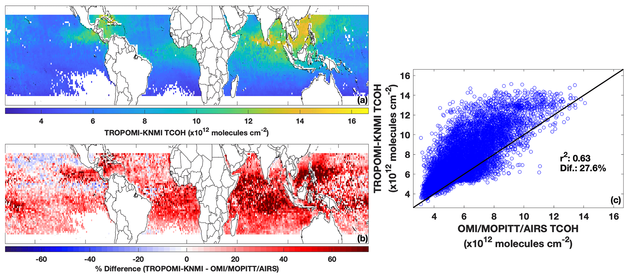
Figure 7 TCOH for May 2018 determined using TROPOMI inputs, including the KNMI NO₂ retrieval (a). The difference between the TROPOMI and multi-satellite product is shown in panel (b). Panel (c) shows the regression of TCOH calculated from TROPOMI against that calculated from retrievals from MOPITT, OMI, and AIRS as well as the percent difference between the two TCOH products.

In general, observations from TROPOMI agree with those from the satellites in Table 1, with the exception of NO₂ and HCHO. Ozone, H₂O_(v), and CO from TROPOMI are highly correlated (r² of 0.85 or higher) and agree within 10 % on average (Fig. S12) with their respective retrievals from OMI, MOPITT, and AIRS. On the other hand, TROPOMI-KNMI NO₂ is systematically higher (145 % on average), and TROPOMI HCHO is 20 % lower than their corresponding OMI retrievals. The higher TCOH from the TROPOMI product is consistent with the increase in NO₂, which would lead to higher secondary production of OH. Further, while TROPOMI-KNMI NO₂ is modestly correlated with OMI NO₂ (r²=0.61), TROPOMI and OMI HCHO are not correlated (r²=0.23), highlighting the difficulty of the HCHO retrieval. Note that we are not seeking to determine which retrieval, if any, is more accurate. We are highlighting the differences to emphasize the impact that systematic differences in retrieval magnitudes of GBRT model inputs can have on the resultant TCOH.

NO₂ drives the differences between the two TCOH products. To determine the impacts of the different TROPOMI inputs on the TCOH product, we individually swapped each TROPOMI input into the OMI–MOPITT–AIRS product, replacing the corresponding input from Table 1. We then determined the difference in TCOH from the OMI–MOPITT–AIRS product that does not include TROPOMI. While this method will not yield the exact contribution from a particular retrieval because of the non-linear nature of OH chemistry, it does yield information about the relative importance of each species. Swapping in TROPOMI CO, H₂O_(v), and O₃ changed TCOH by less than 2 %, while using TROPOMI HCHO increased TCOH by 3 %. In contrast, TROPOMI NO₂ increased TCOH by 29 %, showing that the higher TCOH in the TROPOMI product is driven by differences in NO₂.

The increased TCOH in the TROPOMI product likely results from a combination of differences in the NO₂ retrieval algorithm as well as instrumental differences. Comparison of the KNMI and MINDS retrievals illustrates this point. When compared to OMI, the MINDS NO₂ retrieval is 58 % higher for May 2018, as compared to 145 % higher for the KNMI retrieval. The closer agreement is unsurprising since the MINDS NO₂ uses the same retrieval algorithm as for OMI. Substituting the MINDS NO₂ as an input to the TROPOMI product (TROPOMI-MINDS product) reduces the difference with respect to the OMI–MOPITT–AIRS product to 18 % (Fig. S13). While this is an improvement in agreement, the differences in TCOH as well as the lack of change in r² value still suggest that differences between OMI and TROPOMI unrelated to the retrieval algorithm account for some of the discrepancy. In addition, the training dataset does not take TROPOMI averaging kernels and shape factors into account, which could also contribute to the observed differences.

The results here demonstrate the sensitivity of the methodology to any systematic bias in the input retrievals. As with the random error analysis, the level of uncertainty introduced by these biases is low enough to allow for a meaningful OH product. Despite these differences, the methodology to determine TCOH using machine learning that we have presented here still captures the variability in TCOH, consistent with the ATom evaluation outlined in Sect. 5.1. To reduce the uncertainty of TCOH, better evaluation of NO₂ in the remote atmosphere is needed to determine which retrievals, if any, are accurate.

6 Discussion and recommendations for future observations

The method of estimating clear-sky TCOH presented here has the potential to increase our understanding of the atmospheric oxidation capacity. Because of the long record of observations from MOPITT, OMI, AIRS, and MODIS, we can calculate tropical TCOH from 2005 to the present, and since the methodology is not constrained to a particular satellite, newer satellite missions could extend the dataset beyond the end of these instruments' lifetimes. In addition, this methodology will provide sub-hemispheric information on OH variability, supplementing information available from MCF inversions.

The methodology could be expanded to the extratropics and over land, allowing for global constraints on OH. Expansion over land will likely require additional satellite retrievals, like that of isoprene (Wells et al., 2020), in regions with more complex VOC chemistry than in the remote atmosphere. A higher-resolution TCOH product over land would also likely be feasible because of the increased signal to noise of the NO₂ and HCHO retrievals. Expanding this product beyond the tropics could increase understanding of global CH₄, CO, and VOC trends and variability and allow for a wider range of satellite retrievals as inputs. For example, current and upcoming geostationary air quality satellites such as Sentinel 4, TEMPO (Tropospheric Emissions: Monitoring of Pollution), and GEMS (Geostationary Environment Monitoring Spectrometer) could provide retrievals of most of the necessary inputs to the machine learning model, allowing for the understanding of diurnal variability in TCOH and potentially in the diurnal variability of ozone production (Zhu et al., 2022a).

A similar methodology could likely be used to determine OH at different layers of the atmosphere. Because CH₄ loss is not evenly distributed throughout the tropospheric column, vertically resolved OH would better help inform this process. Vertically resolved OH could also help understand differences in OH drivers in the upper and lower troposphere (Spivakovsky et al., 1990; Lelieveld et al., 2016), which can often be decoupled from the column. While column inputs, such as those discussed here, could be used, the inclusion of vertically resolved satellite retrievals, such as the AIRS H₂O_(v) layers, would provide additional information. Tropospheric O₃ at different atmospheric layers, such as that previously provided by the TES satellite, could also be invaluable here, as O₃ is a large driver of primary OH production.

Satellite-derived OH would also a provide a much-needed, observational constraint on OH variability in global chemistry models. Because the methodology can capture variability in TCOH of both observations and 3-dimensional model output, TCOH trends from a satellite-constrained product could be used to evaluate modeled trends and as well as the spatial variability resulting from events like ENSO. While the satellite-derived OH could not explicitly indicate the cause of differences, the spatial distribution of the differences as well as differences in observed and modeled machine learning model inputs could indicate potential dynamical or emission sources of error in the 3D model.

Further, the combination of the satellite-derived OH and the machine learning model could help identify the impacts of any diagnosed errors in emissions inventories as well as the impacts of unexpected events, such as COVID-19-related shutdowns, on TCOH. For example, if there are significant discrepancies between observed and modeled NO₂ in a specific region of the atmosphere, the satellite NO₂ could be scaled to more closely match the 3D model values and then be input into the machine learning model. The difference in TCOH would then indicate the relative impact of the model error. This would serve as a computationally efficient complement to other methodologies constraining models with observations (e.g., Miyazaki et al., 2020, 2021) to identify the impacts of these errors on the atmospheric oxidation capacity. A similar methodology could be used for unexpected events that significantly impact emissions of OH drivers, allowing for quick determination of their potential impacts on the atmospheric oxidation capacity before emissions inventories could be revised.

While we have shown that the methodology captures the variability of observed OH and generally agrees with observations within measurement uncertainty, it is unclear whether differences result from GBRT model deficiencies or structural differences between the in situ observations and the training dataset. Additional field campaigns with observations of OH and the GBRT model inputs would allow for a more thorough evaluation of both the OH product and the methodology itself. Such a field campaign would need to provide complete tropospheric columns of all species and cover less horizontal distance than the ATom profiles (e.g., from spiral flight patterns). In situ observations of NO₂ without significant interference from NO_x reservoir species are also needed to reduce uncertainty. Alternatively, NO₂ and other species could be measured through aircraft-based remote sensing. Finally, repeated sampling over the same locations for multiple days within a defined area would allow for meaningful statistical analysis while also allowing for the comparison of TCOH columns calculated from satellite observations.

Finally, accuracy of the TCOH product is dependent on the accuracy of the satellite retrievals input into the machine learning model, with the NO₂ retrieval having the largest effect. To reduce the uncertainty of the TCOH product, more information about the accuracy of individual NO₂ retrievals is required. Currently, there is little validation of OMI and TROPOMI NO₂ retrievals in the remote, tropical atmosphere, so it is difficult to assess which retrievals, if any, are correct. Recent efforts, such as the QA4ECV (Quality Assurance for the Essential Climate Variables), to improve NO₂ retrieval algorithms have reduced uncertainty, particularly over land (Boersma et al., 2018), although it is unclear how the accuracy of these retrievals translates to the remote tropics as validation data are still extremely limited. Even retrievals of TROPOMI and OMI made with the same algorithm show differences, suggesting that instrumental differences could also affect the results. Future satellite missions should focus on trying to reduce the uncertainty in NO₂ retrievals, particularly in the remote atmosphere, both through improvements in instrument design and algorithm development.