the Creative Commons Attribution 4.0 License.
the Creative Commons Attribution 4.0 License.
 | 06 Jun 2023
Quantification of oil and gas methane emissions in the Delaware and Marcellus basins using a network of continuous tower-based measurements
Kenneth Davis
Natasha Miles
Scott Richardson
Aijun Deng
Benjamin Hmiel
David Lyon
Thomas Lauvaux
According to the United States Environmental Protection Agency (US EPA), emissions from oil and gas infrastructure contribute 30 % of all anthropogenic methane (CH4) emissions in the US. Studies in the last decade have shown emissions from this sector to be substantially larger than bottom-up assessments, including the EPA inventory, highlighting both the increased importance of methane emissions from the oil and gas sector in terms of their overall climatological impact and the need for independent monitoring of these emissions. In this study we present continuous monitoring of regional methane emissions from two oil and gas basins using tower-based observing networks. Continuous methane measurements were taken at four tower sites in the northeastern Marcellus basin from May 2015 through December 2016 and five tower sites in the Delaware basin in the western Permian from March 2020 through April 2022. These measurements, an atmospheric transport model, and prior emission fields are combined using an atmospheric inversion to estimate monthly methane emissions in the two regions. This study finds the mean overall emission rate from the Delaware basin during the measurement period to be 146–210 Mg CH4 h−1 (energy-normalized loss rate of 1.1 %–1.5 %, gas-normalized rate of 2.5 %–3.5 %). Strong temporal variability in the emissions was present, with the lowest emission rates occurring during the onset of the COVID-19 pandemic. Additionally, a synthetic model–data experiment performed using the Delaware tower network shows that the presence of intermittent sources is not a significant source of uncertainty in monthly quantification of the mean emission rate. In the Marcellus, this study finds the overall mean emission rate to be 19–28 Mg CH4 h−1 (gas-normalized loss rate of 0.30 %–0.45 %), with relative consistency in the emission rate over time. These totals align with aircraft top-down estimates from the same time periods. In both basins, the tower network was able to constrain monthly flux estimates within ±20 % uncertainty in the Delaware and ±24 % uncertainty in the Marcellus. The results from this study demonstrate the ability to monitor emissions continuously and detect changes in the emissions field, even in a basin with relatively low emissions and complex background conditions.
- Article
(4838 KB) - Full-text XML
-
Supplement
(5041 KB) - BibTeX
- EndNote


Methane is a potent greenhouse gas with a global warming potential of 28 over a 100-year period (Forster et al., 2021). Since pre-industrial times, atmospheric methane mole fractions have increased by nearly a factor of 3, contributing to approximately a fourth of the increased radiative forcing due to anthropogenic climate change (Dlugokencky et al., 2011; Myhre et al., 2013). After a brief period during which methane values leveled out from 1999 through 2006, concentrations and growth rates began increasing again in the last decade (Nisbet et al., 2019), renewing concerns of the impact anthropogenic methane emissions will have on warming. Rapid mitigation of these sources has been shown to be a crucial step to achieving climate benchmarks set forth in the Paris Agreement (Saunois et al., 2020; Ocko et al., 2021).
An analysis of pathways to methane mitigation in Ocko et al. (2021) found that the largest economically feasible reductions in methane emissions can be achieved through mitigation strategies in the oil and gas (O&G) sector. In the United States the largest source of anthropogenic methane emissions is from O&G infrastructure, from which leaks and planned releases of natural gas account for more than 30 % of total US anthropogenic methane emissions (US Environmental Protection Agency, 2020). From the years 2008 to 2020, US O&G production increased substantially, with natural gas production increasing by 75 % and oil production increasing by 125 % during the period (US Energy Information Administration, 2021a). Despite substantial increases in O&G infrastructure and production, the US Environmental Protection Agency's (US EPA) bottom-up methane inventory for O&G shows a decadal decline in the overall methane emissions from the sector (Fig. S1 in the Supplement). However, independent top-down analyses of methane emissions from individual well pads (Rella et al., 2015; Robertson et al., 2017; Caulton et al., 2019; Robertson et al., 2020), basins (Karion et al., 2015; Barkley et al., 2017; Peischl et al., 2018; Lin et al., 2021), and regions (Barkley et al., 2019b, 2021) have consistently concluded that the EPA's bottom-up inventory is underestimating emissions from the O&G sector, often by more than 50 % (Alvarez et al., 2018). Recent satellite-driven inversions have come to similar conclusions (Maasakkers et al., 2021; Zhang et al., 2020; Shen et al., 2022), raising further concerns about the accuracy of the bottom-up inventory. With the US recently adopting new policies aimed at reducing methane emissions from the O&G sector (117th Congress, 2022), accurate, precise, and reliable independent monitoring will be necessary to track compliance with established benchmarks.
Various top-down methods currently exist to aid in monitoring emissions of O&G basins, but each has flaws limiting its capabilities for long-term monitoring. Whole-basin aircraft mass balance techniques are a common way to check basin-wide totals (Pétron et al., 2012; Karion et al., 2013; Peischl et al., 2015), measuring methane concentrations upwind and downwind of the basin and converting the change in mass to an emission rate. However, these flights provide only a snapshot of the emissions during the day of the flight rather than serving as a continuous source of monitoring, and assumptions of steady-state winds can lead to the removal of multiple flight days from the dataset if conditions are not met (Schwietzke et al., 2017). Recent developments in airborne spectroscopy have allowed for basin-wide methane quantification by detecting and quantifying individual plumes at the facility level and then scaling up based on an assumed distribution of events (Chen et al., 2022; Cusworth et al., 2022), but this requires assumptions on the total emissions from sources below the detection threshold of the instruments and suffers from a lack of long-term temporal information similar to aircraft mass balance techniques. Satellite-based observations of methane over O&G basins provide a more long-term solution for continuous emissions monitoring when applicable (Zhang et al., 2020; Varon et al., 2022), but this technique struggles in regions with frequent cloud cover, complex terrain, or small signals (Lorente et al., 2023; Shen et al., 2022), limiting its utility in certain O&G basins.
In this study we present an additional possible pathway towards continuous, basin-wide emissions monitoring. Tower-based monitoring networks have been utilized in various urban regions across the world, continuously tracking carbon dioxide and methane emissions from cities as many of them work towards emissions reduction targets (Sargent et al., 2018; Lauvaux et al., 2016; Staufer et al., 2016; Monteiro et al., 2022a). For this work, a tower-based methane monitoring network was designed and implemented in two different O&G basins with the objective of continuously measuring and quantifying regional methane emissions from O&G activity in each basin. We present findings from these networks and discuss advantages and limitations of monitoring regional methane emissions from O&G activity using tower networks.
The objective of this study is to use methane measurements from tower sites in both the Delaware and northeastern Marcellus basins to solve for emissions from O&G sources in each area. Details for the tower network, prior emissions inventories, model setup, and data analysis are provided below.
2.1 Tower network
In the Delaware basin, observations come from a tower network designed to take continuous methane and other trace gas measurements from the western portion of the Permian basin in western Texas and southeastern New Mexico. Picarro cavity ring-down spectroscopy instruments (Picarro, Inc., models G2301, G2401, G2204, and G2132-i) were set up at five sites surrounding the Delaware basin: Carlsbad Caverns National Park (CARL), Maljamar (MALJ), Hobbs (HOBB), Notrees (NOTR), and Fort Stockton (FORT) (Fig. 1). Of the five sites, the instruments at MALJ, HOBB, NOTR, and FORT were installed at tower sites with intake heights between 90 and 130 m a.g.l. (above ground level), with the fifth site CARL first deployed on a rooftop (intake height 4 m a.g.l.) and later a small tower (intake height 9 m a.g.l.). Site CARL is on a ridge approximately 300 m above the elevation of the Permian basin. In the Delaware basin the wind direction varies seasonally, with consistent, strong westerlies in the winter and weaker easterlies in the summer (Fig. S2). As such, the role each tower has is seasonally dependent, with CARL serving as the main upwind tower in winter and MALJ, HOBB, and NOTR being downwind of the basin, while in the summer NOTR and FORT are often the main upwind towers, and CARL becomes the primary downwind tower. Continuous methane mole fraction measurements were taken starting 1 March 2020 and are planned to continue beyond 2023 (Fig. S3). Though observations are taken at all hours of the day, only the daily afternoon average mole fractions are used for analysis (4 h period starting at 20:00 UTC – Universal Coordinated Time; 13:00 CST – Central Standard Time). During these hours, the atmospheric boundary layer height is generally at its deepest and most constant value throughout all seasons, maximizing the likelihood that the measured mole fraction is representative of the full boundary layer column due to strong vertical mixing (Fig. S4). Data collected during instrument or valve malfunctions and during on-site testing were excluded from the calculation of hourly and afternoon averages. Further details regarding tower setup and instrument calibration can be found in Monteiro et al. (2022b).
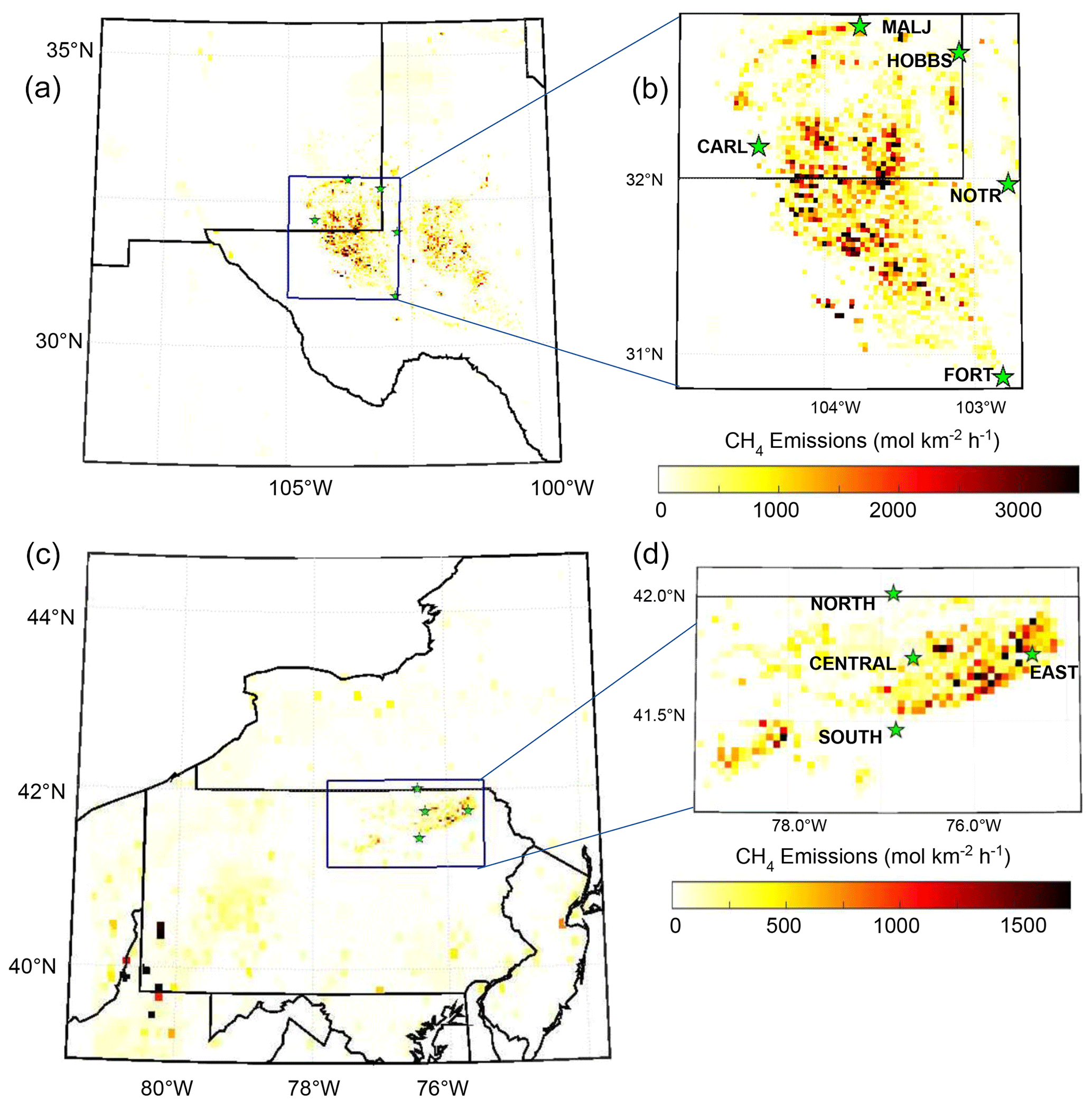
Figure 1(a) A map of emissions within the inner model domain of the WRF-Chem model run for the Delaware basin setup. (b) Emissions within the study area (the region solved for in the inverse analysis). Towers are marked as green stars on the map with their abbreviated names. O&G emissions in the figure are based on the EIME prior. (c) A map of emissions within the inner model domain of the WRF-Chem model run for the Marcellus basin setup. (d) Emissions within the study area (the region solved for in the inverse analysis). Towers are marked as green stars on the map with their abbreviated names. O&G emissions in the figure are based on the production-based prior.
In the Marcellus, observations come from a similarly designed tower network designed to measure methane sources from approximately 4500 high-producing unconventional gas wells in northeastern Pennsylvania (Fig. 1). Instruments were set up at four tower sites starting in May 2015 with intake heights between 46 and 61 m a.g.l., and measurements took place through the end of 2016 when funding for the measurements ended. These tower sites are named after their geographical locations relative to one another: North, East, Central, and South. In the Marcellus, wind directions have a consistent westerly component such that East and Central towers are the primary downwind towers, whereas either North or South serves as an upwind tower depending on whether a northerly or southerly component is present in the wind direction. Daily afternoon average mole fractions (4 h period starting at 18:00 UTC, 13:00 EST – Eastern Standard Time) are used for analysis (Fig. S5), chosen similarly to the Delaware basin based on the timing of when the boundary layer height maximizes and stabilizes during all seasons (Fig. S4). Further details regarding tower setup and instrument calibration can be found in Miles et al. (2018).
The study areas are defined as the areas of O&G production surrounded by the tower networks and are shown in the right panels of Fig. 1, with the Delaware study area defined as the region at 30.83–32.92∘ N, 102.7–105.0∘ W and the Marcellus study area defined as the region at 41.10–42.10∘ N, 75.4–77.5∘ W. Though both of these tower networks are designed to measure emissions from O&G infrastructure, the characteristics of the O&G production within each of the study areas differ greatly. The Delaware basin study area represents an area 230×210 km in size with nearly 50 000 active wells, approximately 80 % of which are classified as oil wells, and contains a mixture of old and new gas infrastructure. By contrast, the Marcellus study area is smaller, at 190×110 km, and only contains 4500 wells, all of which produce only gas. The gas wells in the northeastern Marcellus are on average the highest-producing gas wells in the US, and the total gas produced in the Marcellus study area is nearly equivalent to the gas produced in the Delaware basin, despite the former only having th the number of wells. These two basins lie on the extreme end of gas and oil production and serve as test beds for our ability to monitor different types of O&G basins using tower networks.
2.2 Model setup
Two separate runs of the Weather Research and Forecasting Model with Chemistry (WRF-Chem V3.6.1) were used as an atmospheric transport model to create meteorology fields in the regions surrounding the tower networks and to generate influence functions at each tower site. The WRF model grid configuration used for both regions consists of a gridded 9 km resolution outer domain with a nested 3 km domain centered around the study area (Figs. S6 and S7). A total of 50 vertical terrain-following model layers are used, with 26 model layers below 850 hPa (approximately 1550 m a.g.l.). For the Marcellus model run and the Delaware model run, the North American Regional Research (NARR) model and the ECMWF Reanalysis Fifth-Generation (ERA5) model were respectively used to generate initial and boundary conditions for the simulation (Mesinger et al., 2006; Hersbach et al., 2020). The WRF model is capable of weighting its gridded meteorology towards both the reanalysis data used to drive it (analysis nudging) and local observations that lie within the domain (observational nudging), preventing the model from deviating far from the reanalysis model and observed regional conditions (Stauffer and Seaman, 1994; Lauvaux et al., 2016). Analysis nudging was applied in the 9 km domains, with observational nudging used in both the 9 and 3 km domains. Further details on the setup of the model runs can be found in Barkley et al. (2021).
A Lagrangian particle dispersion model was used in combination with the wind fields and turbulent kinetic energy from the WRF-Chem simulations to generate influence functions for each tower site within the 3 km domains (Uliasz, 1994; Lauvaux et al., 2008, 2012). These influence functions can be combined with a surface emissions map to calculate an expected enhancement at each of the tower sites. A total of 900 particles were released at each tower site each hour in 20 s intervals and traced back in time for 72 h, tracking their interactions with the surface to create a footprint of the area of influence at a tower relative to a given hour of measurements.
2.3 Prior emission inventories
To generate modeled methane enhancements that can be compared to observations from the tower network, a prior methane emissions inventory is required that represents a reasonable first-guess spatial mapping of emissions in the study area. Although the EPA 2012 Gridded Methane Inventory contains information for O&G emissions, emissions are based on infrastructure in 2012 and O&G production in the Permian more than tripled from 2012 to 2020 (Maasakkers et al., 2016; US Energy Information Administration, 2021b), making it outdated to serve as an accurate prior. Therefore, in the Delaware inner model domain, we use the EIME emissions map developed in Zhang et al. (2020), based on the extrapolation of site-level measurements to currently existing O&G infrastructure, to represent our best-guess prior for emissions from O&G sources in the Permian basin. For emissions from O&G sources in Mexico, values derived from Sheng et al. (2018) are used. For the remaining non-O&G anthropogenic sources, the EPA's 2012 Gridded Methane Emissions Inventory (Maasakkers et al., 2016) is used for sources within the US, and EDGAR v4.3.2 is used for sources in Mexico. Overall, 98 % of emissions within the smaller study area confined within the inner model domain originate from O&G sources based on the EIME prior (Fig. S8).
In the Marcellus inner model domain, an O&G emissions inventory for the region is created based on information from the Pennsylvania Department of Environmental Protection (PADEP) Air Emissions Inventory, a bottom-up inventory of emissions from unconventional (horizontally drilled) activity in Pennsylvania. To account for emissions from the remaining conventional (vertically drilled) O&G activity in the state, we use values from the EPA's 2012 Gridded Methane Emissions Inventory oil and gas sectors (Maasakkers et al., 2016), which primarily consist of emissions from conventional activity in the western portion of the state. To prevent the possibility of double-counting unconventional gas emissions in northeastern PA, emissions from the EPA's inventory for the production and gathering sector are zeroed and all O&G emissions from these sectors are assumed to come from unconventional natural gas activity. It is of note that there are fewer than 10 producing conventional wells in the smaller study area confined within the inner model domain, so errors associated with emissions from conventional gas activity would have a marginal impact on results. For anthropogenic emissions from sources other than O&G, the EPA's 2012 Gridded Methane Inventory is used. The primary non-O&G anthropogenic methane emissions come from two landfills in the Scranton–Wilkes-Barre urban corridor and Williamsport in the southeastern and south-central portions of the model domain, respectively, and are not co-located with natural gas activity (Fig. S9). Overall, 55 % of anthropogenic emissions within the study area originate from O&G sources based on the PADEP prior, though this percentage is likely low due to suspected underestimations of O&G emissions from the bottom-up emissions inventory. Though wetland emissions are not included in the prior, WetCHARTs, an ensemble of wetland emission scenarios, shows a mean emission rate in the domain of 3 Mg h−1, which is less than a fourth of the anthropogenic sources in the region (Bloom et al., 2017).
In addition to the main inventories developed for this study, an alternative O&G prior is used for each region to capture the sensitivity of the analysis to the emissions information used. In the Delaware basin, the alternative prior used is the posterior from the satellite-based inversion of the Permian in Zhang et al. (2020) and will be referred to as the Zhang inventory henceforth. To upscale the resolution of the posterior to a prior for our 3 km resolution model grid, emissions from the coarser grid are distributed to the finer grid based on the well count in each of the 3×3 km grids. Though the total O&G emissions in the study area are similar between the EIME and the Zhang inventory, their spatial mappings are very different, with the Zhang inventory emphasizing higher emissions on the western side of the study area near tower CARL (Fig. S10).
For the Marcellus basin, an alternative prior for the study area is developed by attributing O&G emissions at each grid cell equivalent to 0.4 % of the reported average gas production for 2015–2016, as defined by the central estimate of all published gas production loss rates in the northeastern Marcellus (Peischl et al., 2015; Barkley et al., 2017; Caulton et al., 2019). Unlike the Delaware where both priors are similar in magnitude, the alternative O&G prior used for the Marcellus is more than 3 times larger than the PADEP inventory (Fig. S11), which is likely underestimating emissions (Brandt et al., 2014; Alvarez et al., 2018). It should be noted that for most basins, applying a flat loss rate based on production can lead to large spatial flaws in an inventory, as differences in well age, production, and gas composition can affect the production-normalized loss rate by more than an order of magnitude (Omara et al., 2016). However, in the northeastern Marcellus, no significant gas activity existed prior to the regional gas boom around 2010, and as such the existing infrastructure shares similar characteristics that allow a production-normalized emission rate to serve as a suitable spatial mapping of O&G emissions.
2.4 Calculating the observed O&G methane enhancement
By multiplying the influence functions by an emissions inventory, a methane enhancement is calculated at each tower site that represents the total enhancement associated with all sources within the model domain (example: 50 ppb). This value is fundamentally different than the tower observational dataset, which measures the global methane mole fraction (example: 2000 ppb). For the observed and modeled datasets to be comparable, a daily afternoon value that represents the methane mole fraction entering the model domain must be subtracted from the observations. This value is referred to as the background value.
One of the simplest ways to determine the background value for a given afternoon is to select the mole fraction of a tower observation that has had minimal interaction with methane sources within the model domain. For example, the mole fraction value of a tower downwind of zero methane sources within the model domain would be very representative of the methane characteristics of the air mass that entered the model domain and would serve as a good choice for a background value. Yet rarely do such conditions exist in which tower measurements are not impacted at all by sources within the model. Towers upwind of the O&G basin on any given afternoon can still have model enhancements over them, as winds are often not steady throughout the time air travels through the model domain, and plumes from sources that have traveled for hours or even days within the domain can sometimes exist over towers that would otherwise intuitively be thought of us “upwind”. As such, we use two methods to determine which tower would best serve as a background tower for a given afternoon.
The first method is to select the tower with the lowest observed afternoon methane mole fraction. The logic is that the lowest observed methane value would naturally have the smallest influence from local sources within the domain. However, air masses that enter the model domain are not always homogeneous, and the tower with the lowest observed mole fraction may be lowest because it is in a portion of the incoming heterogeneous air mass with low methane relative to the other towers. This can result in a background selection with a low bias.
The second method is to select the tower with the lowest modeled afternoon methane enhancement. The logic is that the tower with the lowest modeled methane enhancement would, by definition, have the smallest influence from sources within the model domain. However, due to transport error in the model as well as spatial errors in the prior inventory, the tower with the lowest modeled enhancement may actually be enhanced by real sources within the domain and have a high measured mole fraction. This can result in a background selection with a high bias.
For each afternoon, we use both of these methods to select a tower as the background tower. With a background tower selected, we take its afternoon mole fraction and subtract the afternoon modeled enhancements at that tower, resulting in a background value that defines the methane mole fraction that is representative of the air mass that entered the model domain. This can be represented through the following equation:
where YbgTower is the observed afternoon methane mole fraction at the identified background tower, XbgTower is the simulated afternoon methane enhancement at the identified background tower, and Ybg is the calculated background value. If the two methods to define a background tower select two different towers, a background value is calculated for each, and their values are averaged together to create a single background value. This background value is subtracted from the observed afternoon methane mole fractions of the downwind towers, producing an “observed methane enhancement” that represents the total observed methane enhancement from sources within the model domain. Finally, modeled enhancements from sources not related to O&G are subtracted from the observed methane enhancement at each downwind tower, producing an observed methane enhancement specific to O&G within the model domain. This process can be written as the following equation:
where YO&G represents the observed afternoon methane enhancements from O&G sources inside the study area, Y is the observed afternoon mole fraction at a downwind tower, and Xother represents the modeled enhancements at the downwind tower from sources other than O&G.
At this stage, the observed methane enhancement from O&G (YO&G) can now be compared directly to the modeled methane enhancement from O&G, and adjustments to the model O&G emissions can be done to create the best match between observed and modeled enhancements. A test on the impacts of six different background selection techniques on the overall results of this study can be found in Sect. S2.
2.5 Inversion methodology
For each basin, we solve for a monthly emissions map that best describes the methane observations measured by the tower network during the period. To do this, a Bayesian inversion is performed to optimize emissions from O&G activity in the study area (Lauvaux et al., 2012; Sheng et al., 2018; Barkley et al., 2021) by minimizing the following cost function:
where yO&G is the observed O&G enhancement inside the domain of interest, x0 and x are the prior and posterior O&G fluxes at 3×3 km resolution, H is the influence function that translates the emissions map (x0) into an enhancement, and R and B are the observation and flux error covariance matrices that control the uncertainty in the observations and the model. Minimizing this equation and solving for the posterior flux map x, the equation can be rewritten as the following:
Further details on the role of each of these terms in solving for the posterior emissions solution can be found in Sect. 2.2 of Barkley et al. (2021).
The inversion is run in monthly intervals, creating a posterior representative of the observations for each month. An average of 70 and 40 downwind afternoon tower observations are used per month in the Delaware and Marcellus inversions, respectively, with monthly fluctuations due to variable downtime across towers in the networks (Fig. S12). For the Delaware inversion, the prior flux (x0) error covariance matrix of the O&G fluxes is assigned to equal 100 % of the magnitude of the source. For the Marcellus inversion, this error is equal to 100 % of the O&G fluxes for the production-based prior and 350 % for the PADEP inventory. This large increase in the error matrix is necessary due to the small initial values of the O&G fluxes in the PADEP prior that would otherwise prevent substantial deviations from their original values. Increasing the flux error covariance matrix for the PADEP prior to 350 % matches the magnitude of the error with the production-based prior, allowing for greater convergence between the two inventories. For both the Delaware and Marcellus inventories, the error covariance matrix is set to zero in all other sources, effectively making any changes from the prior to the posterior the result of changes to the O&G emissions. Furthermore, the region in which the fluxes can be adjusted is limited to the study area shown in Fig. 1. This prevents the inversion from attempting to adjust emissions from the Midland basin in the Permian and the western Marcellus–Utica in the Marcellus, which are both areas that were not intended to be captured based on the design of the tower networks. An e-folding correlation length scale of 5 km is applied to the off-diagonals of B to observe changes between the prior and posterior fluxes over broader areas.
For the observation error covariance matrix R, the model enhancements are first scaled by a constant such that the bias between the observations and model is 0. From there, a constant value is assigned for all observations unique to each month equal to the mean absolute error between the observations and the prior modeled enhancement for that month (Barkley et al., 2021). This technique is done under the assumption that the main source of error between the model and observations is related to errors in transport. Using an R that scales by the mean absolute error results in larger R values during winter months when plumes are larger due to a shallow boundary layer, and thus errors in the transport can produce larger discrepancies between observations and the modeled enhancements (Figs. S10 and S11).
In addition to the inversion settings described above, six additional inversions with unique adjustments were performed for each prior to quantify the sensitivity of the posterior to different choices in the inversion setup. These adjustments include changing the magnitude of the prior to examine its effects on the posterior's magnitude, increasing the error covariance matrix to allow more freedom for the inversion, increasing the correlation length coefficient to force more uniform adjustments to the posterior, adjusting the definition of afternoon hours to include the late morning, and changing the background approach to select the background tower(s) based purely on wind direction. Due to the Marcellus inventory having a prior in which non-O&G sources are not negligible, an additional sensitivity test is performed for that basin, solving for all anthropogenic sources rather than subtracting the non-O&G sources, and then calculating the changes in the posterior solution specific to O&G sources. Descriptions of this sensitivity analysis and its findings can be found in Sect. S1 in the Supplement.
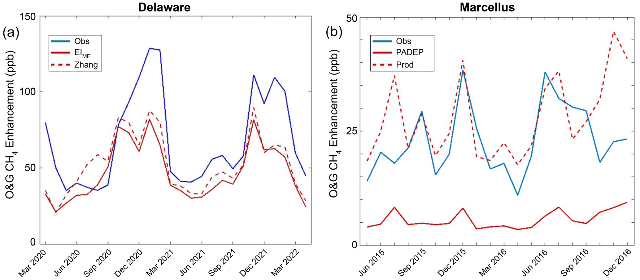
Figure 2(a) Mean monthly afternoon observed methane enhancements from O&G sources within the Delaware study area compared to modeled values using the EIME inventory and the Zhang inventory. (b) Mean monthly afternoon observed methane enhancements within the northeastern Marcellus study area compared to modeled O&G enhancements from the PADEP inventory and the production-based inventory.
3.1 Observed and modeled enhancements
Figure 2 shows the monthly observed and modeled methane enhancements from O&G sources inside the Delaware and northeastern Marcellus study areas. In the Delaware basin, the average observed enhancement varies from 50 ppb during the summer months to 130 ppb in the winter months. This seasonal variability in the Delaware can be seen in both the observations and the model and has two causes unrelated to changes in the emission rate. The main contributor is due to substantial differences in the regional boundary layer height between the summer and winter months, which varies from an average of ∼1000 m in January to 3000 m in July (Fig. S13). The height of the boundary layer affects the depth in which any local enhancements will mix vertically in the atmosphere and thus has an inverse relationship with the size of the signal observed by the tower network. A second, more subtle source of the seasonal variability in the enhancement in the Delaware relates to changes in the wind patterns specific to the region. In the late fall and winter seasons, westerlies are the predominant wind direction, whereas in the late spring and summer, weaker southerlies and easterlies are more prevalent (Fig. S2). This wind shift changes the predominant downwind towers and, as a result of this, the typical surface area of influence associated with these measurements, which results in changes to the average observed enhancement.
With regards to the model priors in the Permian, the EIME and the Zhang emission maps have similar monthly enhancements due to having similar overall emission totals, with the largest differences occurring in summer 2020. This difference is driven by spatial differences in the emissions in the western Delaware basin near tower CARL, which becomes the main downwind tower during this time due to a prolonged period of easterly winds. The higher emissions in the Zhang inventory near this western tower site have a negative impact on its skill at predicting the enhancements there, with an overall mean absolute error of 81 ppb at CARL using the Zhang inventory versus 50 ppb using the EIME prior. These issues along the western portion of the basin result in the EIME performing slightly better overall compared to the Zhang inventory in terms of the mean absolute error and correlation with the observed enhancements (Table S1 in the Supplement). In addition to possible issues in the western portion of the basin, both inventories appear to underestimate the magnitude of the methane enhancements, particularly in the winter months, with observed enhancements during this period greatly exceeding values predicted by either inventory. This large difference could signify genuine increases in the true O&G emissions during the winter months or potential errors in the transport model that are dependent on season.
In the northeastern Marcellus, average observed monthly O&G methane enhancements are much smaller than those in the Delaware, with monthly enhancements ranging between 10 and 35 ppb and no obvious seasonal trend in the observations or the model. The lack of a seasonal trend is related to counteracting effects of boundary layer heights (600 m a.g.l. in winter versus 1800 m a.g.l. in summer) and average wind speeds (10 m s−1 in winter versus 5 m s−1 in summer). The slower winds in summer have a large impact on the Marcellus network due to the proximity of the sources to the tower, creating scenarios in which stagnant summer winds can lead to greater accumulation of methane in the regional boundary layer in the summer months.

Figure 3(a) Prior and posterior monthly O&G methane emission totals for the Delaware basin based on the EIME prior (blue) and Zhang inventory (red) from this study. (b) Prior and posterior monthly O&G methane emission totals for the Marcellus basin based on the production-based prior (blue) and the PADEP prior (red). In both charts, the shaded area represents the minimum and maximum emission rate for each month based on the range of results by adjusting the inversion as described in the sensitivity analysis in Sect. S1, with the darkest grey area showing where the range of emission solutions overlaps between the two priors.
With regards to the performance of the priors in the northeastern Marcellus, a clear discrepancy can be observed between the PADEP prior and the production-based prior, with the former consistently underestimating monthly O&G enhancements by a factor of 3 or greater, whereas the production-based inventory produces enhancements that are slightly higher than observed values (Fig. 2). This discrepancy is expected, as bottom-up inventories of unconventional wells in the Marcellus region have been shown to greatly underestimate empirical results (Barkley et al., 2019a; Caulton et al., 2019), whereas the production-based inventory is based on empirical results using observations from a previous aircraft mass balance campaign in the region (Barkley et al., 2017). In addition to issues with the magnitude of the emissions, there appear to be spatial concerns with the PADEP prior as well (Fig. 1). One of the largest spatial differences between the production-based prior and the PADEP prior is the lack of emissions around Central tower in the PADEP prior, despite that tower being located in an area surrounded by gas infrastructure (Fig. S11). Not coincidentally, Central tower also has the largest difference between the two inventories in terms of correctly capturing the observed gas signal, with a correlation of 0.63 using the production-based prior versus a value of 0.40 using the PADEP prior.
3.2 Inversion results: Delaware basin
Figure 3 shows the resulting emission rates of the monthly inversion performed for the Delaware basin using the mean and range of the monthly emission rate solutions from the inversions performed in the sensitivity analysis. Both priors produce similar results in both the magnitude and trends of the emissions, with the largest emission rates of 220 Mg CH4 h−1 occurring in March and April 2020 when the tower network was established, followed by a sharp and persistent decline in the emission rate down to 130 Mg CH4 h−1 through late summer, then an increase again into winter when it stabilizes through the remainder of 2021 at approximately 160 Mg CH4 h−1, with signs of increasing back to pre-pandemic levels in 2021. The root cause of the nearly 50 % decrease in emissions from March 2020 to September 2020 is unclear but may be related to the tower network measurements coinciding with the onset of the COVID-19 pandemic in late March 2020, when major changes in O&G production and activity were taking place (US Energy Information Administration, 2021a; Lyon et al., 2021). In particular, the timing of the decrease in emissions from April 2020 to September 2020, followed by the gradual rebound, aligns well with data on rig counts in the Permian (US Energy Information Administration, 2021b; Baker Hughes, 2022) (Fig. S14). The drop in emissions correlating with decreasing rig counts may indicate that processes associated with new well drilling, completions, and/or operations may have a disproportionate role in the overall basin-wide emissions. Additional evidence from two aircraft mass balances performed in the Delaware in January and early March 2020 supports the possibility that emissions at the start of 2020 were higher than at any other time during the study period before experiencing a drop in emissions in April and beyond (Lyon et al., 2021). In addition to possible changes throughout the study period caused by the COVID-19 pandemic, a second event occurred in mid-February 2021, when multiple winter storms and below-average temperatures led to disruptions in O&G production across the Permian basin. It is during this month when calculated emission rates are higher than any other period after April 2020. However, calculated emissions had been increasing prior to the multiple winter storm events in February, making it difficult to assess whether the peak in the emission rate in February 2021 was related to disruptions in the gas supply chain or rather a continuation of previous trends heading into the winter months. Regardless of the reason, the increase in emissions is short-lived, and emissions steady out through October 2021, after which they appear to climb again through the remainder of the study period. The increasing emissions occur at a time when both monthly oil and gas production totals were increasing in the Permian and may be related to that change in production (US Energy Information Administration, 2021a).
The range of emission solutions from the sensitivity analysis for each month individually averages ±35 Mg CH4 h−1 (Fig. 3). This range corresponds with a uncertainty range of ±20 % of the mean emission rate. While it is difficult to assign a formal confidence interval to this range, we adopt this range as a level of confidence in our ability to quantify changes in emissions in this basin. Detailed information on the performance of the posterior and sensitivity analysis can be found in the Supplement (Figs. S15 and S16, Tables S1–S5).
Although results from this study and from Lyon et al. (2021) both originate from the same observational dataset, there are some key differences in methodology that result in discrepancies between calculated monthly emissions from the two analyses (Fig. S17). In Lyon et al. (2021), emissions were solved using a scaling factor methodology based on the forward model run enhancements for a smaller, 100×100 km area compared to this study, which uses an inverse methodology based on enhancements derived from influence functions to solve for a much larger domain. The scaling factor methodology forces a single, daily emission rate solution for the entire study region, whereas the inverse methodology is able to account for more complex spatial nuances in the emission field and the error structures of the observations. In addition to differences in the optimization method in which emissions were solved, emissions in the Lyon et al. (2021) study were calculated by averaging afternoon concentrations between 16:00 and 22:59 UTC compared to 20:00–23:59 UTC in this study. For this study the later afternoon times were chosen based on the timing in the transport model runs in which atmospheric boundary layer depth had stabilized at its afternoon peak, whereas between 16:00 and 22:59 UTC, boundary layer growth is actively occurring, increasing from an average of 850 m at 16:00 UTC to 2250 m at 22:00 UTC (Fig. S4). Because the size of local methane enhancements inversely scales with the depth of the boundary layer, this growth by 2.5 times in the boundary layer can create two issues. First, lower boundary layer heights in the late morning would result in larger enhancements in the late morning compared to the afternoon, weighting the overall afternoon observed and modeled enhancement towards whatever enhancements were present during the earlier time period. Second, any errors in the timing of the boundary layer growth would become a substantial source of error in the emissions calculation. For example, the average boundary layer growth between 16:00 and 17:00 UTC is 42 %, so a 1 h error in the timing of that growth would produce a 42 % error in the expected size of the enhancement. Furthermore, along with the differences in selected afternoon hours, the background value methodology selected in Lyon et al. (2021) is less sophisticated than this study, selecting the background only by choosing the tower with the lowest afternoon methane mole fraction. As discussed in Sect. 2.4, this background strategy will produce a low bias in the true background calculation, resulting in larger downwind enhancements and thus a larger emissions solution. The updates applied to the methodology in this paper are developed beyond the initial Lyon et al. (2021) work, and the resulting emissions from this study should be seen as superseding the values from the previous tower analysis.
By averaging the mean monthly solutions from the various inversions performed in the sensitivity analysis, we can create a spatial map of emissions that represents the averaged posterior emissions map for the Delaware basin (Fig. 4). Though the EIME prior and posterior are close in their overall emission rate (175 Mg CH4 h−1 vs. 171 Mg CH4 h−1), certain changes occur consistently in the monthly posterior maps. In particular, methane emissions from the central Delaware basin, which contains much of the newer O&G activity, are reduced by about 20 % compared to the prior. This decrease is canceled out by a moderate increase in the emissions along the southeastern portion of the domain, along with small increases along the perimeter of the domain. This spatial mapping does not agree with the posterior map from Zhang et al. (2020), which substantially increases emissions along the western portion of the domain near the tower CARL. These higher emissions led to large discrepancies and poor correlations with observations at CARL, particularly during the summer months when it is the predominant downwind tower. Performing the tower-based inversion on the Zhang inventory removes the large sources along the western side of the study area and produces a posterior solution more similar to the EIME inventory (Fig. S18). While these spatial inconsistencies may indicate disagreement in the true spatial mapping of the emissions, it must be noted that the time periods of these studies do not overlap (May 2018–March 2019 vs. March 2020–October 2021), so the discrepancies in the spatial mapping could be due to actual changes in the location of emissions over time.

Figure 4Prior, posterior, and difference between the EIME prior and posterior maps in the Delaware study area, averaged across all months based on the mean solution from the inversion sensitivity analysis.
Based on the range of results from the sensitivity analysis in this study, the total average O&G methane emissions in the study area across the various inversions range from 146–210 Mg CH4 h−1, corresponding to a loss rate between 2.5 % and 3.5 % of gas production during the study period, with a best estimate of 2.9 %. Though this number is higher than the national average of 2.3 % reported in Alvarez et al. (2018), it is important to consider that the Permian basin is a major source of oil production, and the loss rate of methane in the region is associated with the production of both natural gas and oil (Allen et al., 2021). Converting the oil produced during the time period to an energy-equivalent amount of natural gas and including it in the loss rate results in an energy-normalized loss rate of 1.1 %–1.5 %. The spatial mapping of the energy-normalized loss rate has extreme variability based on location and correlates strongly with the age and average production of the wells (Figs. S20 and S21). In the northwestern and far eastern areas of the study area where the median age of the wells is more than 20 years, average energy-normalized loss rates typically exceed 5 %, whereas in the center of the study area where the most recent development has taken place, energy-normalized loss rates average less than 1 %. Much of the spatial difference is likely driven by the average energy production per well. Low-producing and marginal wells have been previously shown to have large emission rates relative to their production (Omara et al., 2018, 2022), and the areas with older wells in the Delaware basin have much lower production rates compared to newer activity.
One statistical oddity with the posterior solution for the Delaware basin is the existence of a low bias in the mean model enhancement relative to the observations. The EIME prior starts out with an average modeled enhancement that is 21 ppb lower than the observations. Intuitively, one would expect the posterior solution to increase the emissions to minimize this bias. However, while the posterior solution does reduce the mean absolute error and improve the model–observation correlation, it does not improve the bias (Table S2). This suggests that the inversion does not find that emissions within the basin are responsible for the low bias in the model data. This is further corroborated by the sensitivity test in which the prior emissions are increased by 50 %. Despite the increased prior eliminating the model–observation bias, the posterior solution returns it to a bias of 11 ppb. One possibility could be associated with a biased background selection. If the chosen background value is biased low, all observed downwind enhancements would be increased by this bias, artificially inflating all mean observed enhancements by the bias. These errors would not be fully correctable by the inversion, as the bias would be present in situations in which the footprint of the downwind tower does not overlap with O&G sources in the study area and thus cannot be corrected, leaving the bias to be present in the posterior solution. By selecting the background tower based solely on wind direction (the alternative background approach used in the sensitivity test), the bias in the prior is reduced to 7 ppb, potentially indicating that the default background method used in this study is the source of the bias. However, basing the background on the wind direction produces a mean absolute error and model–observation correlation that is substantially worse compared to using the default background methodology (Table S2). Regardless of the background method selected, the mean posterior emission totals using either approach are within 10 % of each other (Table S7). It is notable that a satellite-based inversion of the Permian basin in Varon et al. (2022) also found a low model bias of similar values when using the Delaware tower network as an independent check on their posterior solution, potentially suggesting that this bias is inherent to challenges specific to the observational dataset in the Delaware basin.
3.3 Assessing errors related to the intermittent characteristic of emissions in the Delaware basin
Recent literature has found that large emitters from O&G infrastructure are constantly shifting spatially on timescales much shorter than our monthly inversion time step (Cusworth et al., 2021) and that large point source emissions can contribute upwards of half of total emissions within a basin (Cusworth et al., 2022; Zavala-Araiza et al., 2015a; Frankenberg et al., 2016; Rutherford et al., 2021). To better understand the errors that could occur from an ever-changing emission field, an observing system simulation experiment (OSSE) was designed to simulate these intermittent sources in our inversion results. Airborne surveys in the Permian basin detected and quantified over 4000 intermittent point source emissions from 2019–2021 (Cusworth et al., 2021, 2022). From this list of emissions, the values of 170 emitters are selected and placed on a daily emissions map distributed randomly in space weighted towards grids with higher emissions from the EIME. The number of intermittent emissions selected for each daily map (170) creates a scenario in which the average total emissions from intermittent sources are equivalent to one-half of the total EIME emissions in the study area based on the concept that up to half of a basin's emissions may originate from large point source emitters (Frankenberg et al., 2016; Cusworth et al., 2022; Zavala-Araiza et al., 2015b; Lyon et al., 2015). This intermittent emissions map is then added to the EIME emissions map with its emissions magnitudes halved. The end result is a randomized daily emission map on which, on average, half of the emissions (88 Mg CH4 h−1) are associated with constant sources from the EIME prior and half are associated with random, sporadic emissions with characteristics observed in field studies. A random map is generated for each day of the year and is multiplied by the influence functions from this study, resulting in a modeled simulation of O&G enhancements in the study area based on these randomized maps. These enhancements are then redefined as the “observed O&G enhancements”, and the inversion is performed using the full EIME emissions map as the prior to solve for these simulated observations and see whether the inversion is still capable of achieving the correct monthly emission rates. This experiment is performed 100 times, with randomly generated daily emission maps for each iteration.
Figure S22 and Table S6 show the results of the OSSE for the Delaware basin. Despite half of the emissions shifting locations daily, the inversion was still able to come within 10 % of the correct monthly total emission rate more than 95 % percent of the time. Additionally, there was little variation in the error across months, indicating that the changing seasonal meteorology in the basin has little influence on the tower network's ability to ascertain the correct total emission rate from these transient sources. The mean absolute error between the pseudo-observed O&G enhancements and the model posterior O&G enhancements ranged between 4 and 7 ppb. This error is substantially smaller than the error observed in the real-world experiment (41 ppb, Table S6), indicating that the intermittent nature of O&G emissions is only a small source of error in solving for monthly emissions and that errors associated with other aspects, such as incorrect model meteorology and errors in the assigned background air mass value, likely play a larger role in the inversion's ability to accurately simulate the observed mole fractions in the basin. For this reason, until errors associated with these major sources can be reduced below the natural variability caused by intermittent emitters, detection and quantification of these short-lived events will be difficult to achieve with a tower network.
3.4 Inversion results: Marcellus basin
Monthly posterior emission rates from the northeastern Marcellus inversion can be seen in Fig. 3. Posterior emission results from both priors show similar temporal trends, but different overall magnitudes, with monthly emission rates close to 14 Mg CH4 h−1 using the PADEP prior versus 22 Mg CH4 h−1 using the production-based prior. The difference in magnitude between these solutions is due to the differences in their starting values; the PADEP prior initiates at a value 3.5 times lower than the production-based prior. The restriction this prior has on the posterior solution can be observed in the sensitivity analysis. Multiplying the production-based prior by 0.5 times and 1.5 times and rerunning the inversion produces a solution that moves towards a centralized value between the two prior ranges, whereas increasing the PADEP prior by 1.5 times and running the inversion still results in a posterior solution that is greater in magnitude than its starting value. The inability of the PADEP prior to reach a point of convergence with the production-based prior, the massive underestimation of the observed enhancement when using the PADEP prior (Fig. 2), and the numerous prior studies that have found emission rates to be much greater than the PADEP inventory (Barkley et al., 2017, 2019a; Caulton et al., 2019; Peischl et al., 2015) suggest that the PADEP inventory is inadequate as a prior for the northeastern Marcellus inversion. For this reason, we choose to focus on the mean and range of solutions from the production-based prior for analysis and disregard the lower values from the PADEP posterior solutions.
Unlike the Delaware inversion, for which longer-term trends were present, deviations from the mean rate in the Marcellus appear more stochastic and short-lived. The lack of long-term trends in the time series may be reflective of the characteristics of the basin during the period. The northeastern Marcellus is entirely a gas basin, with limited flaring typical of oil fields (Elvidge et al., 2013; SkyTruth, 2022; US Energy Information Administration, 2022). Furthermore, the timeframe in which measurements took place in the Marcellus was stable in terms of overall gas production and well development, with no month experiencing greater than a 5 % variation from the monthly mean over the 2-year period and overall well counts remaining constant with time. The monthly range of the posterior solutions from the sensitivity analysis for the production-based prior averages ±5 Mg CH4 h−1 (Fig. 3). This range corresponds to a uncertainty range of ±25 % of the mean emission rate. While it is difficult to assign a formal confidence interval to this range, we adopt this range as a level of confidence in our ability to quantify changes in emissions in this basin.
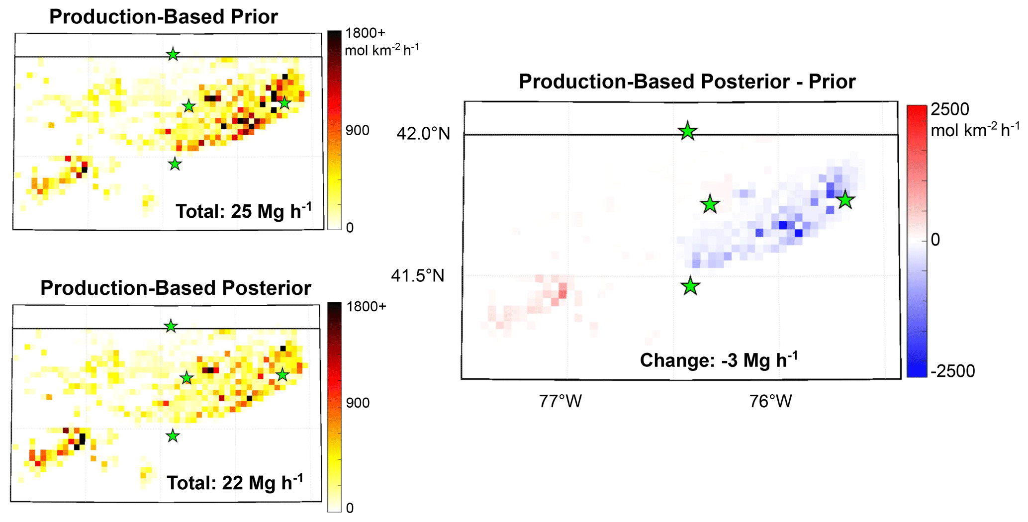
Figure 5Prior, posterior, and difference between the production-based prior and posterior maps in the northeastern Marcellus study area based on the mean solution from the inversion sensitivity analysis.
Based on the range of results from the sensitivity analysis using the production-based prior (Table S4), the total average O&G methane emissions in the northeastern Marcellus study area across the various inversions range from 19 to 28 Mg CH4 h−1, with a best estimate of 22 Mg CH4 h−1 (Table S4). This range corresponds to a regional emission rate of 0.30 %–0.45 % of gas production. The gas loss rate and energy-normalized loss rate in the northeastern Marcellus are equivalent due to a lack of oil production in the region. The loss rate from this study agrees with values observed from top-down aircraft campaigns performed over the study area in 2013 (0.18 %–0.41 %) (Peischl et al., 2015) and 2015 (0.27 %–0.45 %) (Barkley et al., 2017), but it is notably less than values from a major well-sampling study in the region (0.45 %–0.64 %) (Caulton et al., 2019). A satellite inversion that included emission estimates for the northeastern Marcellus from May 2018–February 2020 estimated total emissions in the region to be 3.2 Mg CH4 h−1 (Shen et al., 2022), which is well below the 22 Mg CH4 h−1 from this study. The discrepancy may be related to the magnitude of the prior inventory used in Shen et al. (2022), which assumed regional O&G emissions to be only 1.7 Mg CH4 h−1; this is less than even the PADEP's bottom-up estimate of regional emissions (7 Mg CH4 h−1), possibly restricting the satellite inversion's ability to properly estimate emissions in the northeastern Marcellus. The best estimate of 22 Mg CH4 h−1 from this study represents a threefold increase over values projected by the PADEP prior and demonstrates a significant underestimation of methane emissions from unconventional gas activity in the Pennsylvania Air Quality reports. From the spatial map in Fig. 5, emissions relative to production are lowest in the eastern portion of the domain and see a slight increase relative to the prior in the southwestern quadrant.
3.5 Challenges unique to the Delaware and Marcellus basins
Although the Delaware and Marcellus tower networks were both designed to measure methane emissions from O&G activity, each region has unique circumstances that create different challenges for methane monitoring and emission calculations. The most obvious difference between the two regions is the size of the mole fraction enhancements. The area encompassed by the tower network in the Delaware basin has 8 times more O&G emissions contained within it compared to the northeastern Marcellus basin (171 Mg CH4 h−1 vs. 22 Mg CH4 h−1). Though the emissions in the Delaware cover a larger area and the tower network is farther from the sources, the average observed O&G enhancement at the Delaware downwind tower sites is still 3 times larger than the signal observed from the Marcellus tower network (80 ppb vs. 25 ppb). Generally, a larger signal should result in a more constrained solution, as noise and biases produced by other sources of uncertainty would have less influence on the overall result. However, in the sensitivity analysis performed for this study, both the Delaware and Marcellus basins had similar uncertainty ranges that were approximately 20 % and 25 % of their total emissions, respectively. Furthermore, the statistical performances of the posterior mole fraction solutions in each basin are similar, both with model–observation correlations around 0.6–0.7 and mean absolute errors equal to 50 % of the average O&G enhancement. Despite the discrepancies in the size of the mole fraction enhancements, the tower network and inversion appeared to perform similarly in both basins.
One reason the larger signal in the Delaware may not have translated into a more constrained solution could be related to the magnitude of uncertainty in the background between the two domains. For background selection in both the Delaware and Marcellus studies, 35 % of days had situations in which two different towers could be selected as the background tower based on the methodology described in Sect. 2.4. In the Marcellus domain, the mean difference between the two possible background towers was 14 ppb, while in the Delaware this mean difference was 45 ppb, indicating that background errors may be much larger with the Delaware tower network. Part of the reason for this is likely related to the size of the study areas covered by the two networks. The study area encompassed by the Delaware tower network is 3 times the size of the Marcellus study area, making it less likely that a tower measurement at one end of the domain would be fully representative of the same air mass as a tower on the other end of the domain.
Another difference between the basins that could be an added source of complexity in capturing the signal consistently may relate to the complexity of the emissions within the basins themselves. The northeastern Marcellus basin is exclusively a gas-producing basin. The infrastructure in the region was built almost entirely since the mid-2000s, the gas production per well is the highest in the US, and flaring is minimal compared to basins with significant production of oil and condensate (US Energy Information Administration, 2021a; SkyTruth, 2022; Elvidge et al., 2013). By comparison, the Delaware basin is an oil-rich basin composed of both older and newer infrastructure and in which flaring is commonplace (SkyTruth, 2022; Elvidge et al., 2013). These factors, combined with measurements occurring during the COVID-19 pandemic, may all be sources for sub-monthly temporal variability of the true emissions in the Delaware dataset that are not present in the Marcellus dataset, which would add further error between the observed and modeled methane enhancements.
The expected size of the enhancement, the complexity of the background, and the complexity of the basin are all important to consider when developing a tower network around an O&G basin. This study was successful at constraining methane emissions in both the Delaware and Marcellus basins, but it may be that a tower network surrounding an area with the signal size of the Marcellus and the complexities of the Delaware would struggle to differentiate the mean signal from the noise. Running a forward transport model capable of simulating methane concentrations in an area of interest prior to establishing a tower network (or performing any top-down work) is recommended (Barkley et al., 2017, 2019a). Doing this step prior to setting up the observational network can provide an analytical and visual understanding of expected size, structure, and location of methane plumes from the sources of interest, as well as aid with understanding the complexity of the methane background due to contributions from other sources near the study area. For difficult study areas where the signal-to-noise ratio is expected to be small, having multiple upwind tower sites and a denser and less spatially dispersed tower network should reduce noise in the background and aid in reducing uncertainty in the posterior emissions estimates.
One final source of shared complexity in solving for emissions from these basins comes from errors in the transport. Errors associated with transport will scale with the magnitudes of the mole fraction enhancements. A modeled plume with a 20 % error in the atmospheric boundary layer depth will produce an error in simulated mole fraction enhancement that is 20 % the magnitude of the true enhancement (Barkley et al., 2019a). Likewise, a plume that is measured by a tower site but missed in the model due to wind direction errors will produce an error equivalent to the magnitude of the missed mole fraction enhancement in the plume. For this reason, having a larger enhancement, such as is the case with the Delaware basin, will not necessarily produce a more constrained result if model transport errors are the dominant source of uncertainty in the model solution. This effect may explain why in both the Marcellus and the Delaware, the mean absolute error of the posterior solution is equal to approximately 50 % of the magnitude of the average downwind enhancement (40 and 80 ppb for the Delaware basin, 11 and 25 for the Marcellus). As demonstrated in the OSSE (Sect. 3.3), errors of these magnitudes can make it impossible to capture more subtle aspects of basin emissions, such as the presence of intermittent sources. For this study, customized nested domains and observational and analysis nudging were utilized to reduce transport errors. However, both basins in this study lie in regions with complex terrain and sharp elevation changes in excess of 500 m. A tower network in a basin with simpler meteorology and less complex transport could have improved statistical results relative to those from this study and produce a more tightly constrained posterior solution.
Using methane observations collected from a tower network in the Delaware and Marcellus basins, analysis was performed to learn about emissions from O&G activity in each basin. From the inversion performed for the Delaware tower network, we conclude that emissions in the Delaware basin between March 2020 and April 2022 averaged 146–210 Mg CH4 h−1, or about 1.1 %–1.5 % of the energy-normalized production (2.5 %–3.5 % of gas production). Spatially in the Delaware we find a link between newer, higher-producing O&G infrastructure and lower production-normalized loss rates, a characteristic that has been observed nationally (Omara et al., 2022). Temporal variability was observed during the study period, with the largest emissions occurring just before and at the onset of the COVID-19 pandemic in the US as well as in the winter months. Additionally, by simulating the presence of intermittent emission events inherent to O&G activity, we demonstrate that daily fluctuations to the spatial mapping of emissions in the Delaware basin have no impact on the tower network's ability to resolve the mean monthly emission rates and are not a significant source of uncertainty in full-basin emissions quantification using the tower network.
In the northeastern Marcellus, methane emissions between May 2015 and December 2016 averaged 19–28 Mg CH4 h−1, or about 0.30 %–0.45 % of gas production. Temporal variability in the Marcellus was less apparent than in the Delaware during the study period, possibly due to the stability of gas production at the time and simplicity of the sources. On a monthly timescale, the tower network was able to constrain emissions to ±35 Mg CH4 h−1 in the Delaware (±20 % of the basin emissions) and ±6 Mg CH4 h−1 in the Marcellus (±25 % of the basin emissions).
The overall emission rates found by the tower network analysis in this study compare closely with other top-down aircraft and satellite-based methodologies covering the same regions (Peischl et al., 2015; Barkley et al., 2017; Lyon et al., 2021; Zhang et al., 2020). The alignment of the tower network results using over a year of data, with aircraft mass balance results in particular, illustrates that the “snapshot” approach by aircraft studies may be adequate so long as emissions are stable over time (such as in the Marcellus) or if flights are performed frequently enough to capture long-term trends in temporal variability (such as in the Delaware basin). This study also provides another example of government-developed bottom-up inventories underestimating methane emissions from the O&G sector. In this case, the PADEP inventory of methane emissions from unconventional gas infrastructure underestimates results from the tower network by a factor of 3 (7 Mg CH4 h−1 vs. 19–28 Mg CH4 h−1). Bottom-up inventories can be reconciled with top-down results, as can be observed in the Delaware where the EIME inventory, developed by extrapolating site-level measurements, lies directly in the center of this study's estimate of the Delaware basin (176 Mg CH4 h−1 vs. 146–210 Mg CH4 h−1). Developing methods to correct existing bottom-up inventories should be prioritized now that legislation has been finalized to financially penalize methane emissions from the O&G sector, aiding industry in optimizing emission reduction strategies (117th Congress, 2022) based on more accurate emission factors.
Tower-based observational networks can provide robust, long-term emissions quantification for O&G basins with a level of precision and accuracy that is difficult to achieve with current satellite technologies. In the northeastern Marcellus, the tightly designed tower network is able to continually monitor and quantify methane emissions in a region that would be difficult to capture from satellites due to the small regional signal and frequent cloud cover. Further expansion of the tower networks across other US basins would create an opportunity for continuous monitoring of basin-wide O&G methane emissions, providing near-real-time information on temporal changes in individual basins and serving as a constant check on total emission estimates from bottom-up methodologies. Some basins, of course, may not be accessible for instrumentation with in situ tower networks, while others, like the Permian, may have more favorable conditions for satellite-based measurements, such as frequent clear-sky conditions and large signals. Vigorous co-development of satellite-based and tower-based top-down monitoring is most likely to provide the most robust understanding of global O&G methane emissions.
Hourly averaged tower observations for the Delaware basin can be found at https://doi.org/10.26208/98y5-t941 (Monteiro et al., 2021). Hourly averaged tower observations for the Marcellus basin can be found at https://doi.org/10.18113/D3SG6N (Miles et al., 2017). Influence function data are available upon request.
The supplement related to this article is available online at: https://doi.org/10.5194/acp-23-6127-2023-supplement.
ZB performed the inverse analysis. NM and SR established and managed the observational tower networks. AD ran the forward transport models used to create footprints for the inverse analysis. BH and DL provided information and data specific to the Delaware basin to be used in analysis. KD and TL provided an advisory role with analyzing the data.
The contact author has declared that none of the authors has any competing interests.
Publisher's note: Copernicus Publications remains neutral with regard to jurisdictional claims in published maps and institutional affiliations.
The Delaware tower network and modeling work was completed as part of the Permian Methane Analysis Project project (PermianMAP). The Permian Methane Analysis Project is grateful for the support of Bloomberg Philanthropies, the Corio Foundation, the Grantham Foundation for the Protection of the Environment, the High Tide Foundation, the John D. and Catherine T. MacArthur Foundation, Quadrivium, and the Zegar Family Foundation, as well as MethaneSAT LLC and its donors. The Marcellus tower work was funded by the Department of Energy National Energy Technology Laboratory (DE-FOA-0000894). Computations for this research were performed on The Pennsylvania State University's Institute for Computational and Data Science Roar supercomputer. We thank Carlsbad Caverns and Guadalupe National Park for hosting an instrument. Finally, we thank Bob Barkley for dutifully climbing the hills of northeastern Pennsylvania monthly to restart routers and keep instruments running in exchange for Bingham's pie.
The PermianMAP project has been supported by the Environmental Defense Fund (award no. 224260) and its donors. The Marcellus tower work was funded by the Department of Energy National Energy Technology Laboratory (DE-FOA-0000894).
This paper was edited by Eliza Harris and reviewed by three anonymous referees.
Allen, D. T., Chen, Q., and Dunn, J. B.: Consistent Metrics Needed for Quantifying Methane Emissions from Upstream Oil and Gas Operations, Environ. Sci. Technol. Lett., 8, 345–349, https://doi.org/10.1021/acs.estlett.0c00907, 2021. a
Alvarez, R. A., Zavala-Araiza, D., Lyon, D. R., Allen, D. T., Barkley, Z. R., Brandt, A. R., Davis, K. J., Herndon, S. C., Jacob, D. J., Karion, A., Kort, E. A., Lamb, B. K., Lauvaux, T., Maasakkers, J. D., Marchese, A. J., Omara, M., Pacala, S. W., Peischl, J., Robinson, A. L., Shepson, P. B., Sweeney, C., Townsend-Small, A., Wofsy, S. C., and Hamburg, S. P.: Assessment of methane emissions from the U.S. oil and gas supply chain, Science, 361, 186–188, https://doi.org/10.1126/science.aar7204, 2018. a, b, c
Baker Hughes: Rig Count, https://rigcount.bakerhughes.com/na-rig-count (last access: September 2022), 2022. a
Barkley, Z. R., Lauvaux, T., Davis, K. J., Deng, A., Miles, N. L., Richardson, S. J., Cao, Y., Sweeney, C., Karion, A., Smith, M., Kort, E. A., Schwietzke, S., Murphy, T., Cervone, G., Martins, D., and Maasakkers, J. D.: Quantifying methane emissions from natural gas production in north-eastern Pennsylvania, Atmos. Chem. Phys., 17, 13941–13966, https://doi.org/10.5194/acp-17-13941-2017, 2017. a, b, c, d, e, f, g
Barkley, Z. R., Lauvaux, T., Davis, K. J., Deng, A., Fried, A., Weibring, P., Richter, D., Walega, J. G., DiGangi, J., Ehrman, S. H., Ren, X., and Dickerson, R. R.: Estimating Methane Emissions From Underground Coal and Natural Gas Production in Southwestern Pennsylvania, Geophys. Res. Lett., 46, 4531–4540, https://doi.org/10.1029/2019GL082131, 2019a. a, b, c, d
Barkley, Z. R., Davis, K. J., Feng, S., Balashov, N., Fried, A., DiGangi, J., Choi, Y., and Halliday, H. S.: Forward modeling and optimization of methane emissions in the south central United States using aircraft transects across frontal boundaries, Geophys. Res. Lett., 46, 13564–13573, https://doi.org/10.1029/2019GL084495, 2019b. a
Barkley, Z. R., Davis, K. J., Feng, S., Cui, Y. Y., Fried, A., Weibring, P., Richter, D., Walega, J. G., Miller, S. M., Eckl, M., Roiger, A., Fiehn, A., and Kostinek, J.: Analysis of Oil and Gas Ethane and Methane Emissions in the Southcentral and Eastern United States Using Four Seasons of Continuous Aircraft Ethane Measurements, J. Geophys. Res.-Atmos., 126, e2020JD034194, https://doi.org/10.1029/2020JD034194, 2021. a, b, c, d, e
Bloom, A. A., Bowman, K. W., Lee, M., Turner, A. J., Schroeder, R., Worden, J. R., Weidner, R., McDonald, K. C., and Jacob, D. J.: A global wetland methane emissions and uncertainty dataset for atmospheric chemical transport models (WetCHARTs version 1.0), Geosci. Model Dev., 10, 2141–2156, https://doi.org/10.5194/gmd-10-2141-2017, 2017. a
Brandt, A. R., Heath, G. A., Kort, E. A., O'Sullivan, F., Pétron, G., Jordaan, S. M., Tans, P., Wilcox, J., Gopstein, A. M., Arent, D., Wofsy, S., Brown, N. J., Bradley, R., Stucky, G. D., Eardley, D., and Harriss, R.: Methane Leaks from North American Natural Gas Systems, Science, 343, 733–735, https://doi.org/10.1126/science.1247045, 2014. a
Caulton, D., Lu, J., Lane, H., Buchholz, B., Fitts, J., Golston, L., Guo, X., Li, Q., McSpiritt, J., Pan, D., Wendt, L., Bou-Zeid, E., and Zondlo, M.: Importance of Super-Emitter Natural Gas Well Pads in the Marcellus Shale, Environ. Sci. Technol., 53, 4747–4754, https://doi.org/10.1021/acs.est.8b06965, 2019. a, b, c, d, e
Chen, Y., Sherwin, E. D., Berman, E. S., Jones, B. B., Gordon, M. P., Wetherley, E. B., Kort, E. A., and Brandt, A. R.: Quantifying Regional Methane Emissions in the New Mexico Permian Basin with a Comprehensive Aerial Survey, Environ. Sci. Technol., 56, 4317–4323, https://doi.org/10.1021/acs.est.1c06458, 2022. a
Cusworth, D. H., Duren, R. M., Thorpe, A. K., Olson-Duvall, W., Heckler, J., Chapman, J. W., Eastwood, M. L., Helmlinger, M. C., Green, R. O., Asner, G. P., Dennison, P. E., and Miller, C. E.: Intermittency of Large Methane Emitters in the Permian Basin, Environ. Sci. Technol. Lett., 8, 567–573, https://doi.org/10.1021/acs.estlett.1c00173, 2021. a, b
Cusworth, D. H., Thorpe, A. K., Ayasse, A. K., Stepp, D., Heckler, J., Asner, G. P., Miller, C. E., Yadav, V., Chapman, J. W., Eastwood, M. L., Green, R. O., Hmiel, B., Lyon, D. R., and Duren, R. M.: Strong methane point sources contribute a disproportionate fraction of total emissions across multiple basins in the United States, P. Natl. Acad. Sci. USA, 119, e2202338119, https://doi.org/10.1073/pnas.2202338119, 2022. a, b, c, d
Dlugokencky, E. J., Nisbet, E. G., Fisher, R., and Lowry, D.: Global atmospheric methane: budget, changes and dangers, Philos. T. Roy. Soc. A, 369, 2058–2072, 2011. a
Elvidge, C. D., Zhizhin, M., Hsu, F.-C., and Baugh, K. E.: VIIRS nightfire: Satellite pyrometry at night, Remote Sens., 5, 4423–4449, 2013. a, b, c
Forster, P., Storelvmo, T., Armour, K., Collins, W., Dufresne, J.-L., Frame, D., Lunt, D., Mauritsen, T., Palmer, M., Watanabe, M., Wild, M., and Zhang, H.: The Earth's energy budget, climate feedbacks, and climate sensitivity, in: book section 7, Cambridge University Press, Cambridge, UK and New York, NY, USA, https://doi.org/10.1017/9781009157896.009, 2021. a
Frankenberg, C., Thorpe, A. K., Thompson, D. R., Hulley, G., Kort, E. A., Vance, N., Borchardt, J., Krings, T., Gerilowski, K., Sweeney, C., Conley, S., Bue, B. D., Aubrey, A. D., Hook, S., and Green, R. O.: Airborne methane remote measurements reveal heavy-tail flux distribution in Four Corners region, P. Natl. Acad. Sci, USA, 113, 9734–9739, https://doi.org/10.1073/pnas.1605617113, 2016. a, b
Hersbach, H., Bell, B., Berrisford, P., Hirahara, S., Horányi, A., Muñoz-Sabater, J., Nicolas, J., Peubey, C., Radu, R., Schepers, D., Simmons, A., Soci, C., Abdalla, S., Abellan, X., Balsamo, G., Bechtold, P., Biavati, G., Bidlot, J., Bonavita, M., De Chiara, G., Dahlgren, P., Dee, D., Diamantakis, M., Dragani, R., Flemming, J., Forbes, R., Fuentes, M., Geer, A., Haimberger, L., Healy, S., Hogan, R. J., Hólm, E., Janisková, M., Keeley, S., Laloyaux, P., Lopez, P., Lupu, C., Radnoti, G., de Rosnay, P., Rozum, I., Vamborg, F., Villaume, S., and Thépaut, J.-N.: The ERA5 global reanalysis, Q. J. Roy. Meteorol. Soc., 146, 1999–2049, https://doi.org/10.1002/qj.3803, 2020. a
Karion, A., Sweeney, C., Pétron, G., Frost, G., Michael Hardesty, R., Kofler, J., Miller, B. R., Newberger, T., Wolter, S., Banta, R., Brewer, A., Dlugokencky, E., Lang, P., Montzka, S. A., Schnell, R., Tans, P., Trainer, M., Zamora, R., and Conley, S.: Methane emissions estimate from airborne measurements over a western United States natural gas field, Geophys. Res. Lett., 40, 4393–4397, https://doi.org/10.1002/grl.50811, 2013. a
Karion, A., Sweeney, C., Kort, E. A., Shepson, P. B., Brewer, A., Cambaliza, M., Conley, S. A., Davis, K., Deng, A., Hardesty, M., Herndon, S. C., Lauvaux, T., Lavoie, T., Lyon, D., Newberger, T., Pétron, G., Rella, C., Smith, M., Wolter, S., Yacovitch, T. I., and Tans, P.: Aircraft-Based Estimate of Total Methane Emissions from the Barnett Shale Region, Environ. Sci. Technol., 49, 8124–8131, https://doi.org/10.1021/acs.est.5b00217, 2015. a
Lauvaux, T., Uliasz, M., Sarrat, C., Chevallier, F., Bousquet, P., Lac, C., Davis, K. J., Ciais, P., Denning, A. S., and Rayner, P. J.: Mesoscale inversion: first results from the CERES campaign with synthetic data, Atmos. Chem. Phys., 8, 3459–3471, https://doi.org/10.5194/acp-8-3459-2008, 2008. a
Lauvaux, T., Schuh, A. E., Uliasz, M., Richardson, S., Miles, N., Andrews, A. E., Sweeney, C., Diaz, L. I., Martins, D., Shepson, P. B., and Davis, K. J.: Constraining the CO2 budget of the corn belt: exploring uncertainties from the assumptions in a mesoscale inverse system, Atmos. Chem. Phys., 12, 337–354, https://doi.org/10.5194/acp-12-337-2012, 2012. a, b
Lauvaux, T., Miles, N. L., Deng, A., Richardson, S. J., Cambaliza, M. O., Davis, K. J., Gaudet, B., Gurney, K. R., Huang, J., O'Keefe, D., Song, Y., Karion, A., Oda, T., Patarasuk, R., Razlivanov, I., Sarmiento, D., Shepson, P., Sweeney, C., Turnbull, J., and Wu, K.: High-resolution atmospheric inversion of urban CO2 emissions during the dormant season of the Indianapolis Flux Experiment (INFLUX), J. Geophys. Res.-Atmos., 121, 5213–5236, https://doi.org/10.1002/2015JD024473, 2016. a, b
Lin, J. C., Bares, R., Fasoli, B., Garcia, M., Crosman, E., and Lyman, S.: Declining methane emissions and steady, high leakage rates observed over multiple years in a western US oil/gas production basin, Sci. Rep., 11, 1–12, 2021. a
Lorente, A., Borsdorff, T., Martinez-Velarte, M. C., and Landgraf, J.: Accounting for surface reflectance spectral features in TROPOMI methane retrievals, Atmos. Meas. Tech., 16, 1597–1608, https://doi.org/10.5194/amt-16-1597-2023, 2023. a
Lyon, D. R., Zavala-Araiza, D., Alvarez, R. A., Harriss, R., Palacios, V., Lan, X., Talbot, R., Lavoie, T., Shepson, P., Yacovitch, T. I., Herndon, S. C., Marchese, A. J., Zimmerle, D., Robinson, A. L., and Hamburg, S. P.: Constructing a Spatially Resolved Methane Emission Inventory for the Barnett Shale Region, Environ. Sci. Technol., 49, 8147–8157, https://doi.org/10.1021/es506359c, 2015. a
Lyon, D. R., Hmiel, B., Gautam, R., Omara, M., Roberts, K. A., Barkley, Z. R., Davis, K. J., Miles, N. L., Monteiro, V. C., Richardson, S. J., Conley, S., Smith, M. L., Jacob, D. J., Shen, L., Varon, D. J., Deng, A., Rudelis, X., Sharma, N., Story, K. T., Brandt, A. R., Kang, M., Kort, E. A., Marchese, A. J., and Hamburg, S. P.: Concurrent variation in oil and gas methane emissions and oil price during the COVID-19 pandemic, Atmos. Chem. Phys., 21, 6605–6626, https://doi.org/10.5194/acp-21-6605-2021, 2021. a, b, c, d, e, f, g, h
Maasakkers, J. D., Jacob, D. J., Sulprizio, M. P., Turner, A. J., Weitz, M., Wirth, T., Hight, C., DeFigueiredo, M., Desai, M., Schmeltz, R., Hockstad, L., Bloom, A. A., Bowman, K. W., Jeong, S., and Fischer, M. L.: Gridded National Inventory of U.S. Methane Emissions, Environ. Sci. Technol., 50, 13123–13133, https://doi.org/10.1021/acs.est.6b02878, 2016. a, b, c
Maasakkers, J. D., Jacob, D. J., Sulprizio, M. P., Scarpelli, T. R., Nesser, H., Sheng, J., Zhang, Y., Lu, X., Bloom, A. A., Bowman, K. W., Worden, J. R., and Parker, R. J.: 2010–2015 North American methane emissions, sectoral contributions, and trends: a high-resolution inversion of GOSAT observations of atmospheric methane, Atmospheric Chemistry and Physics, 21, 4339–4356, https://doi.org/10.5194/acp-21-4339-2021, 2021. a
Mesinger, F., DiMego, G., Kalnay, E., Mitchell, K., Shafran, P. C., Ebisuzaki, W., Jović, D., Woollen, J., Rogers, E., Berbery, E. H., Ek, M. B., Fan, Y., Grumbine, R., Higgins, W., Li, H., Lin, Y., Manikin, G., Parrish, D., and Shi, W.: North American Regional Reanalysis, B. Am. Meteorol. Soc., 87, 343–360, https://doi.org/10.1175/BAMS-87-3-343, 2006. a
Miles, N. M., Martins, D. K., Richardson, S. J., Lauvaux, T., Davis, K. J., Haupt, B. J., and Rella, C.: In-situ tower atmospheric methane mole fraction and isotopic ratio of methane data, Marcellus Shale Gas Region, Pennsylvania, USA, Penn State Datacommons [data set], https://doi.org/10.18113/D3SG6N, 2017. a
Miles, N. L., Martins, D. K., Richardson, S. J., Rella, C. W., Arata, C., Lauvaux, T., Davis, K. J., Barkley, Z. R., McKain, K., and Sweeney, C.: Calibration and field testing of cavity ring-down laser spectrometers measuring CH4, CO2, and δ13CH4 deployed on towers in the Marcellus Shale region, Atmos. Meas. Tech., 11, 1273–1295, https://doi.org/10.5194/amt-11-1273-2018, 2018. a
Monteiro, V., Miles, N. L., Richardson, S. J., Barkley, Z. R., Haupt, B. J., and Davis, K. J.: Permian Basin: in-situ tower greenhouse gas data, Penn State Datacommons [data set], https://doi.org/10.26208/98y5-t941, 2021. a
Monteiro, V., Miles, N., Richardson, S., Turnbull, J., Karion, A., Kim, J., Mitchell, L., Lin, J., Sargent, M., Wofsy, S., Vogel, F., and Davis, K. J.: The impact of the COVID-19 lockdown on greenhouse gases: a multi-city analysis of in situ atmospheric observations, Environ. Res. Commun., 4, 041004, https://doi.org/10.1088/2515-7620/ac66cb, 2022a. a
Monteiro, V. C., Miles, N. L., Richardson, S. J., Barkley, Z., Haupt, B. J., Lyon, D., Hmiel, B., and Davis, K. J.: Methane, carbon dioxide, hydrogen sulfide, and isotopic ratios of methane observations from the Permian Basin tower network, Earth Syst. Sci. Data, 14, 2401–2417, https://doi.org/10.5194/essd-14-2401-2022, 2022b. a
Myhre, G., Shindell, D., Bréon, F.-M., Collins, W., Fuglestvedt, J., Huang, J., Koch, D., Lamarque, J.-F., Lee, D., Mendoza, B., Nakajima, T., Robock, A., Stephens, G., Takemura, T., and Zhang, H.: Anthropogenic and Natural Radiative Forcing, in: book section 8, Cambridge University Press, Cambridge, UK and New York, NY, USA, 659–740, https://doi.org/10.1017/CBO9781107415324.018, 2013. a
Nisbet, E. G., Manning, M. R., Dlugokencky, E. J., Fisher, R. E., Lowry, D., Michel, S. E., Myhre, C. L., Platt, S. M., Allen, G., Bousquet, P., Brownlow, R., Cain, M., France, J. L., Hermansen, O., Hossaini, R., Jones, A. E., Levin, I., Manning, A. C., Myhre, G., Pyle, J. A., Vaughn, B. H., Warwick, N. J., and White, J. W. C.: Very Strong Atmospheric Methane Growth in the 4 Years 2014–2017: Implications for the Paris Agreement, Global Biogeochem. Cy., 33, 318–342, https://doi.org/10.1029/2018GB006009, 2019. a
Ocko, I. B., Sun, T., Shindell, D., Oppenheimer, M., Hristov, A. N., Pacala, S. W., Mauzerall, D. L., Xu, Y., and Hamburg, S. P.: Acting rapidly to deploy readily available methane mitigation measures by sector can immediately slow global warming, Environ. Res. Lett., 16, 054042, https://doi.org/10.1088/1748-9326/abf9c8, 2021. a, b
Omara, M., Sullivan, M. R., Li, X., Subramanian, R., Robinson, A. L., and Presto, A. A.: Methane Emissions from Conventional and Unconventional Natural Gas Production Sites in the Marcellus Shale Basin, Environ. Sci. Technol., 50, 2099–2107, https://doi.org/10.1021/acs.est.5b05503, 2016. a
Omara, M., Zimmerman, N., Sullivan, M. R., Li, X., Ellis, A., Cesa, R., Subramanian, R., Presto, A. A., and Robinson, A. L.: Methane Emissions from Natural Gas Production Sites in the United States: Data Synthesis and National Estimate, Environ. Sci. Technol., 52, 12915–12925, https://doi.org/10.1021/acs.est.8b03535, 2018. a
Omara, M., Zavala-Araiza, D., Lyon, D. R., Hmiel, B., Roberts, K. A., and Hamburg, S. P.: Methane emissions from US low production oil and natural gas well sites, Nat. Commun., 13, 2085, https://doi.org/10.1038/s41467-022-29709-3, 2022. a, b
117th Congress: H.R.5376 – Inflation Reduction Act of 2022, https://www.congress.gov/bill/117th-congress/house-bill/5376/text (last access: June 2023), 2022. a, b
Peischl, J., Ryerson, T. B., Aikin, K. C., de Gouw, J. A., Gilman, J. B., Holloway, J. S., Lerner, B. M., Nadkarni, R., Neuman, J. A., Nowak, J. B., Trainer, M., Warneke, C., and Parrish, D. D.: Quantifying atmospheric methane emissions from the Haynesville, Fayetteville, and northeastern Marcellus shale gas production regions, J. Geophys. Res.-Atmos., 120, 2119–2139, https://doi.org/10.1002/2014JD022697, 2015. a, b, c, d, e
Peischl, J., Eilerman, S. J., Neuman, J. A., Aikin, K. C., de Gouw, J., Gilman, J. B., Herndon, S. C., Nadkarni, R., Trainer, M., Warneke, C., and Ryerson, T. B.: Quantifying Methane and Ethane Emissions to the Atmosphere From Central and Western U.S. Oil and Natural Gas Production Regions, J. Geophys. Res.-Atmos., 123, 7725–7740, https://doi.org/10.1029/2018JD028622, 2018. a
Pétron, G., Frost, G., Miller, B. R., Hirsch, A. I., Montzka, S. A., Karion, A., Trainer, M., Sweeney, C., Andrews, A. E., Miller, L., Kofler, J., Bar-Ilan, A., Dlugokencky, E. J., Patrick, L., Moore Jr., C. T., Ryerson, T. B., Siso, C., Kolodzey, W., Lang, P. M., Conway, T., Novelli, P., Masarie, K., Hall, B., Guenther, D., Kitzis, D., Miller, J., Welsh, D., Wolfe, D., Neff, W., and Tans, P.: Hydrocarbon emissions characterization in the Colorado Front Range: A pilot study, J. Geophys. Res.-Atmos., 117, D04304, https://doi.org/10.1029/2011JD016360, 2012. a
Rella, C. W., Tsai, T. R., Botkin, C. G., Crosson, E. R., and Steele, D.: Measuring Emissions from Oil and Natural Gas Well Pads Using the Mobile Flux Plane Technique, Environ. Sci. Technol., 49, 4742–4748, https://doi.org/10.1021/acs.est.5b00099, 2015. a
Robertson, A. M., Edie, R., Snare, D., Soltis, J., Field, R. A., Burkhart, M. D., Bell, C. S., Zimmerle, D., and Murphy, S. M.: Variation in Methane Emission Rates from Well Pads in Four Oil and Gas Basins with Contrasting Production Volumes and Compositions, Environ. Sci. Technol., 51, 8832–8840, https://doi.org/10.1021/acs.est.7b00571, 2017. a
Robertson, A. M., Edie, R., Field, R. A., Lyon, D., McVay, R., Omara, M., Zavala-Araiza, D., and Murphy, S. M.: New Mexico Permian Basin measured well pad methane emissions are a factor of 5–9 times higher than US EPA estimates, Environ. Sci. Technol., 54, 13926–13934, 2020. a
Rutherford, J. S., Sherwin, E. D., Ravikumar, A. P., Heath, G. A., Englander, J., Cooley, D., Lyon, D., Omara, M., Langfitt, Q., and Brandt, A. R.: Closing the methane gap in US oil and natural gas production emissions inventories, Nat. Commun., 12, 4715, https://doi.org/10.1038/s41467-021-25017-4, 2021. a
Sargent, M., Barrera, Y., Nehrkorn, T., Hutyra, L. R., Gately, C. K., Jones, T., McKain, K., Sweeney, C., Hegarty, J., Hardiman, B., Wang, J. A., and Wofsy, S. C.: Anthropogenic and biogenic CO2 fluxes in the Boston urban region, P. Natl. Acad. Sci. USA, 115, 7491–7496, https://doi.org/10.1073/pnas.1803715115, 2018. a
Saunois, M., Stavert, A. R., Poulter, B., Bousquet, P., Canadell, J. G., Jackson, R. B., Raymond, P. A., Dlugokencky, E. J., Houweling, S., Patra, P. K., Ciais, P., Arora, V. K., Bastviken, D., Bergamaschi, P., Blake, D. R., Brailsford, G., Bruhwiler, L., Carlson, K. M., Carrol, M., Castaldi, S., Chandra, N., Crevoisier, C., Crill, P. M., Covey, K., Curry, C. L., Etiope, G., Frankenberg, C., Gedney, N., Hegglin, M. I., Höglund-Isaksson, L., Hugelius, G., Ishizawa, M., Ito, A., Janssens-Maenhout, G., Jensen, K. M., Joos, F., Kleinen, T., Krummel, P. B., Langenfelds, R. L., Laruelle, G. G., Liu, L., Machida, T., Maksyutov, S., McDonald, K. C., McNorton, J., Miller, P. A., Melton, J. R., Morino, I., Müller, J., Murguia-Flores, F., Naik, V., Niwa, Y., Noce, S., O'Doherty, S., Parker, R. J., Peng, C., Peng, S., Peters, G. P., Prigent, C., Prinn, R., Ramonet, M., Regnier, P., Riley, W. J., Rosentreter, J. A., Segers, A., Simpson, I. J., Shi, H., Smith, S. J., Steele, L. P., Thornton, B. F., Tian, H., Tohjima, Y., Tubiello, F. N., Tsuruta, A., Viovy, N., Voulgarakis, A., Weber, T. S., van Weele, M., van der Werf, G. R., Weiss, R. F., Worthy, D., Wunch, D., Yin, Y., Yoshida, Y., Zhang, W., Zhang, Z., Zhao, Y., Zheng, B., Zhu, Q., Zhu, Q., and Zhuang, Q.: The Global Methane Budget 2000–2017, Earth Syste. Sci. Data, 12, 1561–1623, https://doi.org/10.5194/essd-12-1561-2020, 2020. a
Schwietzke, S., Pétron, G., Conley, S., Pickering, C., Mielke-Maday, I., Dlugokencky, E. J., Tans, P. P., Vaughn, T., Bell, C., Zimmerle, D., Wolter, S., King, C. W., White, A. B., Coleman, T., Bianco, L., and Schnell, R. C.: Improved Mechanistic Understanding of Natural Gas Methane Emissions from Spatially Resolved Aircraft Measurements, Environ. Sci. Technol., 51, 7286–7294, https://doi.org/10.1021/acs.est.7b01810, 2017. a
Shen, L., Gautam, R., Omara, M., Zavala-Araiza, D., Maasakkers, J. D., Scarpelli, T. R., Lorente, A., Lyon, D., Sheng, J., Varon, D. J., Nesser, H., Qu, Z., Lu, X., Sulprizio, M. P., Hamburg, S. P., and Jacob, D. J.: Satellite quantification of oil and natural gas methane emissions in the US and Canada including contributions from individual basins, Atmos. Chem. Phys., 22, 11203–11215, https://doi.org/10.5194/acp-22-11203-2022, 2022. a, b, c, d
Sheng, J.-X., Jacob, D. J., Turner, A. J., Maasakkers, J. D., Sulprizio, M. P., Bloom, A. A., Andrews, A. E., and Wunch, D.: High-resolution inversion of methane emissions in the Southeast US using SEAC4RS aircraft observations of atmospheric methane: anthropogenic and wetland sources, Atmos. Chem. Phys., 18, 6483–6491, https://doi.org/10.5194/acp-18-6483-2018, 2018. a, b
SkyTruth: Flaring Maps and Data, https://skytruth.org/flaring/ (last access: March 2022), 2022. a, b, c
Staufer, J., Broquet, G., Bréon, F.-M., Puygrenier, V., Chevallier, F., Xueref-Rémy, I., Dieudonné, E., Lopez, M., Schmidt, M., Ramonet, M., Perrussel, O., Lac, C., Wu, L., and Ciais, P.: The first 1-year-long estimate of the Paris region fossil fuel CO2 emissions based on atmospheric inversion, Atmos. Chem. Phys., 16, 14703–14726, https://doi.org/10.5194/acp-16-14703-2016, 2016. a
Stauffer, D. R. and Seaman, N. L.: Multiscale Four-Dimensional Data Assimilation, J. Appl. Meteorol. Clim., 33, 416–434, https://doi.org/10.1175/1520-0450(1994)033<0416:MFDDA>2.0.CO;2, 1994. a
Uliasz, M.: Lagrangian particle dispersion modeling in mesoscale applications, in: Environmental Modeling, Vol. II, edited by: Zannetti, P., Computational Mechanics Publications, Southampton, UK, ISBN 978-1-85312-281-1, 1994. a
US Energy Information Administration: Natural Gas Gross Withdrawls and Production, https://www.eia.gov/dnav/ng/hist/n9070us2m.htm (last access: December 2021), 2021a. a, b, c, d
US Energy Information Administration: Drilling Productivity Report: Permian Region, https://www.eia.gov/petroleum/drilling/pdf/permian.pdf (last access: 30 March 2021), 2021b. a, b
US Energy Information Administration: Annual Natural Gas Vented and Flared, https://www.eia.gov/dnav/ng/ng_prod_sum_a_EPG0_VGV_mmcf_a.htm (last access: March 2022), 2022. a
US Environmental Protection Agency: Inventory of U.S. Greenhouse Gas Emissions and Sinks: 1990–2018, https://www.epa.gov/ghgemissions/inventory-us-greenhouse-gas-emissions-and-sinks (last access: August 2020), 2020. a
Varon, D. J., Jacob, D. J., Hmiel, B., Gautam, R., Lyon, D. R., Omara, M., Sulprizio, M., Shen, L., Pendergrass, D., Nesser, H., Qu, Z., Barkley, Z. R., Miles, N. L., Richardson, S. J., Davis, K. J., Pandey, S., Lu, X., Lorente, A., Borsdorff, T., Maasakkers, J. D., and Aben, I.: Continuous weekly monitoring of methane emissions from the Permian Basin by inversion of TROPOMI satellite observations, Atmos. Chem. Phys. Discuss. [preprint], https://doi.org/10.5194/acp-2022-749, in review, 2022. a, b
Zavala-Araiza, D., Lyon, D., Alvarez, R. A., Palacios, V., Harriss, R., Lan, X., Talbot, R., and Hamburg, S. P.: Toward a functional definition of methane super-emitters: Application to natural gas production sites, Environ. Sci. Technol., 49, 8167–8174, https://doi.org/10.1021/acs.est.5b00133, 2015a. a
Zavala-Araiza, D., Lyon, D. R., Alvarez, R. A., Davis, K. J., Harriss, R., Herndon, S. C., Karion, A., Kort, E. A., Lamb, B. K., Lan, X., Marchese, A. J., Pacala, S. W., Robinson, A. L., Shepson, P. B., Sweeney, C., Talbot, R., Townsend-Small, A., Yacovitch, T. I., Zimmerle, D. J., and Hamburg, S. P.: Reconciling divergent estimates of oil and gas methane emissions, P. Natl. Acad. Sci. USA, 112, 15597–15602, https://doi.org/10.1073/pnas.1522126112, 2015b. a
Zhang, Y., Gautam, R., Pandey, S., Omara, M., Maasakkers, J. D., Sadavarte, P., Lyon, D., Nesser, H., Sulprizio, M. P., Varon, D. J., Zhang, R., Houweling, S., Zavala-Araiza, D., Alvarez, R. A., Lorente, A., Hamburg, S. P., Aben, I., and Jacob, D. J.: Quantifying methane emissions from the largest oil-producing basin in the United States from space, Sci. Adv., 6, eaaz5120, https://doi.org/10.1126/sciadv.aaz5120, 2020. a, b, c, d, e, f