the Creative Commons Attribution 4.0 License.
the Creative Commons Attribution 4.0 License.
 | 02 Jun 2023
Divergent convective outflow in large-eddy simulations
Holger Tost
Upper-tropospheric outflow is analysed in cloud-resolving large-eddy simulations. Thereby, the role of convective organization, latent heating, and other factors in upper-tropospheric divergent-outflow variability from deep convection is diagnosed using a set of more than 80 large-eddy simulations because the outflows are thought to be an important feedback from (organized) deep convection to large-scale atmospheric flows; perturbations in those outflows may sometimes propagate into larger-scale perturbations.
Upper-tropospheric divergence is found to be controlled by net latent heating and convective organization. At low precipitation rates isolated convective cells have a stronger mass divergence than squall lines. The squall line divergence is the weakest (relative to the net latent heating) when the outflow is purely 2D in the case of an infinite-length squall line. At high precipitation rates the mass divergence discrepancy between the various modes of convection reduces. Hence, overall, the magnitude of divergent outflow is explained by the latent heating and the dimensionality of the outflow, which together create a non-linear relation.
- Article
(5246 KB) - Full-text XML
-
Supplement
(2808 KB) - BibTeX
- EndNote


Organized deep moist convection is not only a substantial precipitation source over the tropics and mid-latitudes but also a driver of the global atmospheric circulation due to its conversion of potential energy into kinetic and moist static energy. This energy conversion is achieved by so-called latent heating: the condensation of water vapour warms rising air parcels while they move upwards, expand, and cool. The warming tendency of latent heating opposes the stronger cooling tendency (expansion) and provides (positive) buoyancy. The positive buoyancy is the fuel to the moist convection that can keep it running, resulting in accumulation and further organizing. Once organized systems of deep moist convection (from now on referred to as convective systems) have formed, they feed back onto the background atmospheric circulation. The background atmospheric circulation is hardly affected by tiny convective systems composed of one or two cumulonimbus clouds. On the other hand, the mesoscale circulation can be entirely disturbed and even dominated by convective systems of sufficiently large size and intensity (Houze, 2004, 2018); in the case of so-called mesoscale convective systems (MCSs) a complete re-organization of the atmospheric flow around the MCS can happen. In other words, large systems with higher precipitation rates introduce an on average stronger feedback to the large-scale atmospheric flow (intuitively); i.e. the feedback is expected to increase with the precipitation intensity (or, equivalently, the net latent heating). Consequently, the net latent heating can be used to quantify the intensity of convective systems. The feedback onto the background circulation also sometimes has significant consequences for downstream developments of the atmospheric flow (e.g. Rodwell et al., 2013; Clarke et al., 2019a, b).
An increase of the flow feedback strength with the amount of net latent heating is supported by the simplified linearized gravity wave model described in Bretherton and Smolarkiewicz (1989), Nicholls et al. (1991), Pandya et al. (1993), and Mapes (1993). The principles behind this linear gravity-wave-modelling approach have additionally been used for simulations of the flow feedback from squall lines by Pandya and Durran (1996). Furthermore, the model has also been used in a very different set-up to study flow adjustments to localized heating by Bierdel et al. (2018). Bretherton and Smolarkiewicz (1989) studied gravity wave responses to such heat sources with a linearized model that supports gravity waves. Their linear model reveals increasing convectively induced circulation with an increasing latent heat source. The gravity wave adjustment signal propagates away from the convective system, but comparatively strong upper-tropospheric outflow is maintained around the location of the initialized latent heat pulse. Moreover, their model describes how point and line sources generate different outflow responses and how responses depend on vertical wavenumber; in other words, the outflow may depend on the organization of the convection (including storm geometry). Extensions of the linear model by Bretherton and Smolarkiewicz (1989) were later used to understand preferential locations of convective initiation, e.g. in the tropics (Lane and Reeder, 2001; Stechmann and Majda, 2009; Lane and Zhang, 2011; Grant et al., 2018), and to understand error propagation associated with differential heating in a rotational set-up (Bierdel et al., 2017). The linearized model by Bretherton and Smolarkiewicz (1989) can serve as a benchmark for the much more complex irrotational cloud-resolving and large-eddy simulations presented here (for most important predictions of the gravity wave model, here partly used as assumptions, see Bretherton and Smolarkiewicz, 1989; Bierdel et al., 2017, 2018).
Over the last decade, studies on predictability have suggested that differential upper-tropospheric flow variability induced by organized convective systems can impact the predictability of weather (e.g. Rodwell et al., 2013; Baumgart et al., 2019). Hence, the main objective of this study is to understand and diagnose the upper-tropospheric outflow variability and feedback of organized convective systems to their surroundings quantitatively for large-eddy simulations. More specifically, the upper-tropospheric mean lateral acceleration over a control volume, as diagnosed with the mass divergence, is connected to the net latent heating. Analysing a control simulation; an ensemble; and tailored, physically perturbed experimental simulations, this study systematically assesses the effect of net latent heating, convective momentum transport, and convective organization on the divergent outflow of convective systems. The divergence sets in as a horizontal wind compensation for the vertical acceleration of convective upward airflows, accompanied by a high pressure anomaly aloft. Such a high pressure anomaly aloft exists as a consequence of abundant mass aloft.
Ensembles and physical perturbations are applied to the following selected organizational modes of convection: a supercell, regular multicells, and a squall line. The latter class is further sub-divided into two categories (finite-length and infinite-length squall lines). Convective momentum transport is purposely switched off or adjusted by ±50 %. Additional physical perturbations are applied to the aforementioned four basic modes of convection (scenarios) to test specific hypotheses and to improve the quantification of the impact of latent heating.
Large-eddy simulations are suitable for the assessment because of the explicitly resolved turbulence and cloud-scale processes represented in those simulations. Therefore, they can be assumed to represent the convective processes in a reliable way (e.g. Bryan et al., 2003).
The structure of this paper is as follows: in Sect. 2 the model set-up (Sect. 2.1), initial conditions for four prototypes of convection, and corresponding convective environments (both in Sect. 2.2) are described. Furthermore, all perturbation types (including ensemble configuration) are covered in this section (Sect. 2.3), and the analysis window is described (Sect. 2.4). In Sect. 3 the evolution of convective cells is first discussed for the reference simulations. Thereby, each of the four prototypes of convection is introduced separately (Sect. 3.1). This part is followed by an analysis of the vertical motion caused by the convective adjustment. The next part discusses the internal variability in the investigated set-up using the ensemble (Sect. 3.3). Furthermore, suitable vertical masks of the convergence and divergence are investigated in that section. After defining all the constraints, a dataset with integrated outflow divergence patterns can be created in Sect. 3.4. That dataset sheds light onto the relationship between latent heating and upper-tropospheric divergence. The paper ends with a discussion and a conclusion section.
2.1 Model set-up
The simulations presented in this study are conducted with the cloud-resolving model CM1 version 19.8 (Bryan, 2019). The default horizontal grid size is 120 km by 120 km, with a default simulation time of 2 hours (9600dt). The vertical extent of the domain is 20 km. A sponge layer exists in the upper 5 km, which damps upward-propagating gravity waves. Output is stored per 5 min interval. The simulations are run in large-eddy-simulation (LES) mode at m and dz=100 m by default. In addition, extra simulations are run with additional grids where m, m and km. In the latter two, the vertical grids are adjusted to 250 and 500 m intervals. In one last simulation with an adjusted resolution, dz is set to 200 m.
In LES mode, a turbulent kinetic energy (TKE) scheme after Deardorff (1980) handles the subgrid turbulence. For the microphysics, the default CM1 scheme is used (the two-moment scheme of Morrison et al. (2009)). Boundary conditions of the simulations are of the non-periodic, open type. Hence, derivatives of any quantity are set to 0 at the boundaries in every direction: an infinite reservoir of inflow air is theoretically available to the convective systems. As a consequence, reflection of wave signals can also occur at the boundaries. For more details on the model settings (dynamics and physics), we also refer to Groot and Tost (2023).
2.2 Environmental conditions
The initial thermodynamics are prescribed using the profile of Weisman and Klemp (1982) (Fig. A1 in Appendix A), a standard in CM1. Two basic local potential temperature perturbations have been set at t=0 to trigger convective cells with various kinds of organization. Furthermore, the initial wind profiles are varied at t=0 to realize systems that manifest with a certain organizational mode of convection, numbered 1–3 (see the left side of Fig. A1 in Appendix A; Rotunno et al., 1988; Weisman and Klemp, 1982; Bryan, 2019; and Bryan's CM1 code). Each of the four combinations of local temperature perturbations and wind profiles is introduced below. These prescribed profiles establish the four modes of convection. An overview of all the scenarios introduced in this section is shown in Fig. 1.
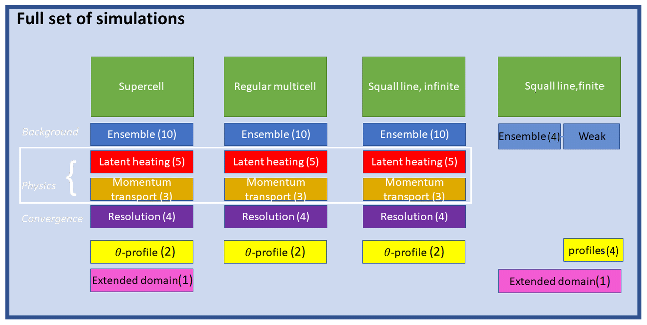
Figure 1Overview of all CM1 experiments done in this study. The four scenarios represented in the columns of the display have been introduced in Sect. 2.2. These green boxes with white captions show each of the four prototypes of convection that we use, with a list of experiment groups following in the column below each of them. Below the column header, the perturbations applied to each scenario are represented and are discussed in the order of display (downward; Sect. 2.3). Here, the white text represents the regular basis set of perturbation experiments applied to the first three modes of convection, and the black font represents irregularities among the experiments, tailored at specific modes of convection and robustness testing. In the last column, “weak” denotes the ensemble band corresponding to the other three scenarios, and “profile” denotes the wide ensemble band, which corresponds to θ profile perturbations in the other three scenarios (Sect. 2.3.1 and 2.3.3).
2.2.1 Supercell
A supercell scenario is constructed by applying an initial warm-bubble disturbance. The warm bubble is initialized around the centre of the domain, with a radius of 10 km in the horizontal. It has a bell-shaped amplitude, with a maximum of 1 K at the origin, and z=1.4 km. The warm bubble forces an upward motion in the domain centre, which, in combination with the high convective available potential energy (CAPE), leads to the growth of strong convective cells.
A strong wind shear profile (1, see Fig. A1 in Appendix A) induces a supercell structure. u gradually increases from easterly winds of 12.5 at the surface to 18.5 m s−1 from the west at the interface between the layer of wind shear and that of unsheared winds, located at z=6000 m in the reference case (Weisman and Klemp, 1982). This combination of strong easterly and westerly winds kept the convective system centred within the domain throughout its evolution. The v wind varied from −2 at the surface to +2 m s−1 at and above that same interface.
2.2.2 Regular multicell
A regular multicell is generated in the same warm-bubble initiation scenario as the supercell case.
Moderate wind shear is applied in combination with the warm-bubble scenario, leading to ordinary regular-multicell convection. However, the easterly inflow at the surface is set to 11 m s−1, while u increases to +3 m s−1 at the interface height located at 2.5 km altitude (adjusted from Rotunno et al., 1988; 2, Fig. A1 in Appendix A). Again, the wind profile is designed to keep the convective system relatively centred within the domain throughout its evolution.
2.2.3 Infinite-length squall lines
An infinite-length squall line is constructed with a cold-pool-damming scenario, in which, west of the y axis, a −6 K potential temperature perturbation is implemented at the surface. This perturbation decreases linearly with height to 0 at a fixed level of z=2.5 km. The upward motion that initializes convection is generated at the border between the air masses in the west and the east. The combination of high CAPE and the moderate shear profile perpendicular to this border leads to a strong line of convective cells.
A moderate wind shear is applied, similarly to the regular-multicell scenario. With this moderate shear, the u component of the wind varies linearly from 12.5 m s−1 of easterly inflow at the surface to a weak westerly flow of 1.5 m s−1 above the top of the shear layer (Fig. A1), which is set at m for this scenario in the reference run (adjusted from Rotunno et al., 1988; 3, Fig. A1 in Appendix A). As in the other two modes of convection, v increases from −2 to +2 m s−1 over the 2500 m deep low-level shear layer.
2.2.4 Finite-squall-line simulations
Despite the substantial similarity to the infinite squall line, this additional class of organized convective systems is constructed to obtain convective cells arranged in a line but with more potential for outflow in the y dimension locally (at least at the squall line edges). This meridional outflow is substantially damped in an infinite-length squall line. Most of the conditions are identical to the infinite-length-squall-line simulations (described above). The main difference is a modification of the initial potential temperature perturbation in the cold-pool-damming scenario: in the central region of the domain, it maximizes at 6 K at the surface, but this surface maximum decreases outward to 0 K near the meridional boundaries of the domain (Fig. A2 in Appendix A illustrates the y–z shape of the profile). The quantities of interest are separately diagnosed over a central region (comparable to the infinite squall line) and an outer region in the finite-length squall lines (on both the northern and southern ends) for this scenario.
2.3 Perturbations
2.3.1 Ensemble perturbations
To test the robustness of the results, an ensemble is constructed in the following way and for each scenario accordingly: the altitude of the interface between the layers where shear is initially present and absent is perturbed (symbol zi). Thereby, the maximum deviation within the ensemble is 5 % from the reference zi,ref. Corresponding extreme deviation values for zi are 2500−127 m and 6000−304 m, with an ensemble mean deviation of 2.7 % from the reference altitude. Relative magnitudes of the perturbations are equal for both shear profiles and, hence, all storm modes.
Ensemble perturbations for the finite-length squall lines (Sect. 2.2.4) are set up in a slightly adjusted way compared to the other three scenarios: four perturbations are generated as a narrow ensemble band where the depth of the initial shear layer is adjusted, similarly as for the infinite squall line. On top of that, four additional ensemble members are generated with stronger initial condition perturbations: one with a 1 km deeper cold pool, one with a deeper (climatologically more realistic) shear layer, and two with a 4 and 7.5 K maximum in terms of the potential temperature perturbation in the domain centre at the surface, referred to as a wide ensemble band.
Ensemble perturbations provide a background scatter for the natural variability of upper-tropospheric divergence within close proximity of the control runs, as caused by small variations in initial conditions. After applying interface perturbations, winds are interpolated to the native vertical grid length of the corresponding simulation (100 m).
2.3.2 Physics perturbations
Two types of physics perturbations are applied. These perturbations are applied for a comparison to the control simulation of each of the three basic modes of convection (Sect. 2.2.1, 2.2.2 and 2.2.3, three left columns of Fig. 1). The constant of the latent heating is adjusted to 60 %, 80 %, 90 %, 110 %, and 120 % of its actual value. This approach has been selected to serve as a proxy for perturbed cloud and microphysics tendencies (e.g. condensation and evaporation) or CAPE without perturbing any of the other physics and the initial environment within the model. Precipitation rates in simulations with an adjusted latent-heating constant are naturally evaluated, with the latent-heating constant adjusted correspondingly in any conversion.
The vertical advection term in both horizontal momentum equations has been adjusted to 0 %, 50 %, and 150 % of its actual magnitude in another set of experiments to perturb the convective momentum transport. This is done to determine the direct effect of the convective-momentum-transport process on upper-tropospheric divergent outflows. The perturbation is similar to creating an artificial source and/or sink term of horizontal momentum at locations with strong convective motion, which is driven by tendencies caused by vertical gradients in horizontal momentum. Systematic non-linear effects on the mass divergence are detectable if processes other than the intensity of the convection affect mass divergence. Additionally, the role of other parameters such as convective organization and convective momentum transport for the upper-tropospheric divergence can be determined by the comparisons between simulations.
2.3.3 Adjusted low-level temperature perturbations
The dataset obtained with simulations introduced in Sect. 2.2 is complemented with additional simulations in which the strength of the potential temperature disturbances (warm bubble(s) or cool-pool damming) has been adjusted. These modifications result in slightly stronger (weaker) triggering, and hence, slightly stronger (weaker) convective cells would be expected compared to the other ensemble simulations. The configuration is as follows: the initial perturbations were halved or otherwise slightly modified using scaled superpositions of the cold-pool and warm-bubble initiations.
2.3.4 Simulations at extended domains
The domain size that has been chosen in this study is on the small end for studying the feedback from convective cells to their environment, especially for the supercells and squall lines and during the last half an hour of the simulations. In the regular-multicell simulations, however, the limited domain size should be of no concern in this regard: the convective cells cover only a limited fraction of the 120 × 120 km domain.
To test the effective limitations of the restricted domain and more robustly determine the patterns in our dataset (and herewith strengthen the conclusions), one supercell simulation and one finite-length-squall-line simulation are conducted at an extended domain (200 km by 200 km). The simulation time is extended to 160 min, but the analysis window is restricted to the two time intervals until 120 min. For the finite squall line, the large-domain-simulation configuration is not identical to the reference squall line simulation but uses the conditions for an ensemble member with reduced potential temperature perturbations (maximum 4 K only). This configuration is selected to prevent too much additional convective initiation (secondary) with convective precipitation. Such secondary convective initiation is partially located further away from the squall line. The additional convective initiation makes the evolution of the system less comparable to the ensemble simulations in the reference domain.
2.4 Spatial and temporal analysis windows
Diagnostics that represent latent heating by precipitation, upper divergent outflow, and convective momentum transport are evaluated over two separate time intervals. The first time interval ends after 75 min for the squall lines and after 90 min for the regular multicells and supercells. Diagnostics are also evaluated over the second time interval, running from the end of the first interval until the end of the simulation (120 min). This approach with two time intervals creates temporal subsamples. In the first interval's subsamples, effects close to the selected box boundary are relatively unimportant. On the other hand, such effects have a comparatively stronger impact on the diagnostics during the second time interval. Comparison between the two intervals helps to determine the relevance of, for instance, the propagation of gravity waves influencing the larger-scale environment.
Furthermore, a restricted rectangular horizontal area within the whole domain is selected, over which diagnostics are averaged spatially, further limiting boundary effects. The exact extent of the boxes is depicted in Sect. 3.2 that follows.
In this section, the development of the convective systems is described from an introductory point of view by illustrating the simulated reflectivity and describing the evolution of the precipitation systems (Sect. 3.1). This is done for the control simulation of each of the four modes of convection separately. Once the horizontal distribution of the convective heat sources and the region of flow adjustment is known (Sect. 3.1 and 3.2; see also Fig. S1 and Sect. S1 in the Supplement), the last requirement for the box analysis and diagnosis of the upper-tropospheric mass divergence from the convective systems is delineating the vertical extent over which the divergent outflows develop (Sect. 3.3). Finally, this section is concluded with the dataset of diagnosed mass divergence and net latent heating for all the simulations and both time intervals, where the mass divergence is based on the horizontal and vertical extent of the box (Sect. 3.4). That dataset bridges the gap to the discussion that follows.
3.1 Evolution of the convective cells
Figure 2 depicts the temporal evolution of the four convective systems in the control simulation together with their corresponding simulated patterns of radar reflectivity.
3.1.1 Supercell
The initial warm bubble is a source of buoyant air around the origin, which can freely ascend. Part of it develops into a deep convective cell, and in the conditions of high shear, it organizes itself as a supercell. After 25 min, the cell develops, and simulated radar echoes appear at 3 km altitude (Fig. 2, left column). The cell stretches out strongly in the east–west direction under the condition of a deep-layer shear larger than 30 m s−1. A hook echo appears after about 45 min in a southern cell, about 10 km west of the origin, with an antisymmetric cell as its northern counterpart. The southern hook echo starts accelerating southeastward and thereby still gains size. On the western flank, initiation of much smaller convective cells sets in after about 85 min.
3.1.2 Regular multicell
From the warm bubble initialized at the origin, a convective cell is able to develop right next to the origin, as in the supercell simulations (Fig. 2, second column). This is a consequence of weak upper-level flow and strong surface inflow with high CAPE values, as given by the Weisman and Klemp (1982) initial conditions and a buoyant warm bubble.
After 25 min of simulation, the first echo signals appear at z=3 km, directly below melting level. A first convective cell remains small during the first hour, with a size of 10 km by 20 km in the horizontal direction and maximum reflectivity around 60–65 dBz. A small cold pool develops on the downdraught side (west). During the next output time steps, the precipitation system remains contiguous but also develops two cores (around and just after 60 min), namely a southerly cell and a northerly cell. Herewith a two-cell system, a multicell, has developed.
3.1.3 Infinite-length squall line
In the infinite-length-squall-line simulations, deep convection develops along the cold-pool edge, which sits on the y axis (Fig. 2, third column). Convective initiation occurs as an upward motion is triggered at the interface between warm air to the east and cool near-surface air in the west. With substantial amounts of CAPE, shear helps to organize the convective storms along the y axis.
The first precipitation cells appear along the y axis after 15 min. A secondary phase of convective initiation occurs a few kilometres ahead of the main squall line after 30–40 min of simulation time, which is more extensively discussed in Groot and Tost (2023). Newly initiated convective storms exceed reflectivities of 55 dBz, with values up to about 65 dBz locally. This is followed by an onset of eastward displacement of the line of convective cells.
The evolution of the squall line ensemble spread is discussed very extensively in Groot and Tost (2023). The key finding is that the essential developments for the ensemble spread occur with the secondary convective initiation, with subsequent differences in cold-pool acceleration within the ensemble.
3.1.4 Finite squall line
The finite squall line starts precipitating after 15 min over a length of about 50 km along the y axis (Fig. 2, last column). After 20 min, reflectivities above 65 dBz already appear in the model output, and the precipitating region grows in each horizontal direction. Cellular structures are not yet present but start appearing after 30 min of simulation time. By this time, its length is about 75 km, centred at the origin.
While the core region maintains its position near the centre of the domain, an extension of the squall line at both ends ( km) adjusts the geometry of the convective system to an arch-shaped line after 60–65 min. Simultaneously, some convective initiation occurs locally, west of km at km. These small cells live for a maximum of 5–10 min. The associated precipitation accumulation is negligible compared to the rest of the squall line (initial conditions were selected to reduce the size and duration of cells as much as possible on purpose).
With the development of the arching geometry, the simulated reflectivity signal strengthens, and the convectively active area in the outer regions (close to the northern and southern boundaries) increases as well. The squall line centre region starts to accelerate eastward and moves to about 15–20 km east of the origin over the last 40 min of the simulation. However, this acceleration is mostly restricted to a 30 km region around y=10 km.
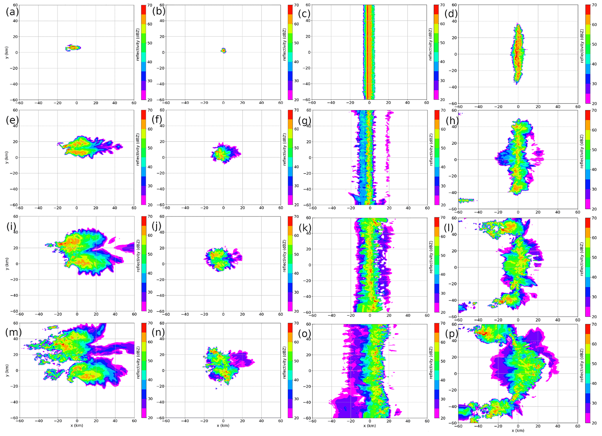
Figure 2Simulated radar reflectivity at 3 km height in the control simulation for each of the four modes of convection. From left to right: supercell (a, e, i, m), regular multicell (b, f, j, n), infinite-length squall line (c, g, k, o), and finite-length squall line (d, h, l, p). From top to bottom, time increases by 30 min (a, b, c, d), 60 min (e, f, g, h), 90 min (i, j, k, l), and 120 min (m, n, o, p).
Cumulative precipitation
The precipitation cells in all four modes of convection do not move far from their original position near the origin, as displayed in each of the panels of Fig. S1 in the Supplement. As the divergent outflows could reasonably be assumed to be collocated with cumulonimbus clouds (the regions of diabatic heating) and their close proximity and thus with the precipitation signal, net outflow has to (mostly) stick to that region near the central part of the domain. That suggests that an integration over a subdomain of the simulation domain suffices for rigorous assessment of outflow magnitudes in the simulation dataset.
3.2 Vertical motion
Figure 3 shows the vertical velocity at a level near the tropopause (within 0.5 km). The boxes over which further diagnostic quantities are integrated are also outlined accordingly as black rectangles. The simulations are split into the following two time intervals, as mentioned in Sect. 2.4: the first interval before the snapshot in Fig. 3 and the second interval, covering the part of the simulation afterwards. The box is chosen such that the flow effect of the convection through rippling in the wave signal at the tropopause level is still limited to the region (mostly) within that horizontal extent. By the time of the snapshot in the figure, only a fraction of the longwave gravity wave signal left the region of the box.
Comparing the four modes of convection, Fig. 3 shows clear contrasts. The supercell simulation (panel a) has a large region over which shortwave signals occur near the tropopause in comparison to the regular multicell. The box size over which outflow is diagnosed has to be sufficiently large that it covers the adjustment region of shortwave gravity wave activity. On the other hand, shortwave variability only occurs in an oval that is restricted to a comparatively smaller region in the regular-multicell simulation (panel b). For a fair comparison, the supercell and regular-multicell integration boxes are set over the same spatial extent relative to the initial warm bubble. A region where near-tropopause boundary reflection effects (as a result of the open boundary conditions) are suspected to occur can be identified in the infinite-length squall line simulation; specifically, regions away from the centre (y=0) have a wider zonal extent (about km) over which shortwave w variability is strong (namely at and y>40) compared to the central region. That pattern in w is not present in the display of the finite-length squall line as a consequence of the arch shape, which only covers a restricted part of the domain.
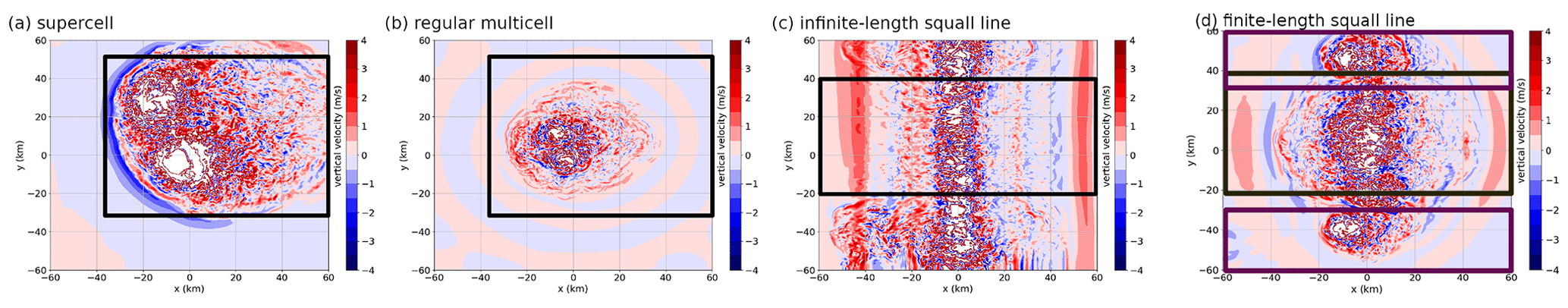
Figure 3Vertical velocity at tropopause level after 90 min for the control simulations of (a) the supercell simulation and (b) the regular-multicell simulation and after 75 min (c) for the infinite-length-squall-line simulation and (d) the finite-length-squall-line simulation. The thick black outline of the rectangle defines the outer region of the horizontal box over which diagnostics are integrated, and the time stamp that belongs to it defines the end point of the first integration interval. That stamp corresponds to the start of the second integration interval as well. Areas that mostly exceed ±4 m s−1 indicate direct convective motion, which means that an updraught (downdraught) core is present locally.
The patterns of vertical motion as a consequence of gravity waves and convection occurring in the middle troposphere are discussed in further detail in Sect. S2 of the Supplement. This is the level where the wave amplitude of the fastest mode of gravity waves maximizes.
3.3 Divergence profiles
Figure 4 shows the time evolution (x axis) of the vertical divergence profiles (y axis) for each of the four basic types of convective organization (starting from t=5 min). Initially, the convection has not developed. It requires about 30 min before intense convection develops, as can be visualized with the selected threshold and corresponding colour scale in the figure. Note that the colour scales of the isosurfaces and the isolines use different values to allow for a distinction between the pattern of individual ensemble members and the ensemble mean value of strong divergence. In the top and bottom rows, strong convergent low-level (z<3 km) signals start to exceed the isoline threshold after about 45 min (±20 min). With a slight delay (about 15–20 min), strong signals of mass divergence set in and stick to a layer between 8 and 13 km, around and just below the tropopause.The mass divergence (convergence) signals in the regular multicell both set in after 1 h in the upper (lower) troposphere. Afterwards, they expand their vertical extent with time. In this set of simulations, the upper-tropospheric divergence also sticks to the 8–13 km layer. The low-level convergence expands quite a lot after about 1.5 h so as to nearly cover the full lower half of the troposphere.
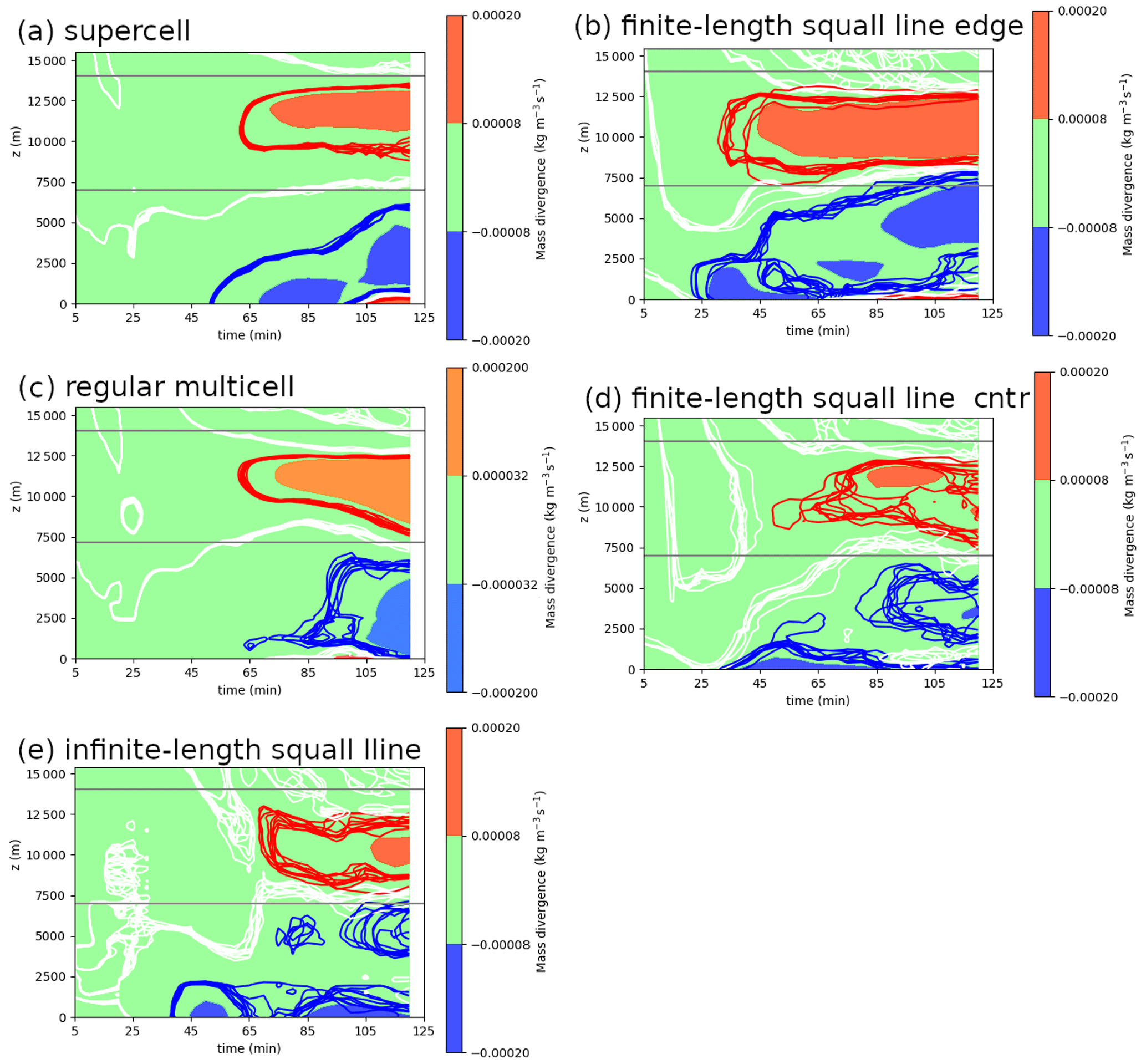
Figure 4Time evolution of mass divergence (convergence) as a function of height for three basic modes of convection averaged over the ensemble (filled) and for the individual members (spaghetti contours – blue: kg m−3 s−1, white: 0 kg m−3 s−1 (i.e. neutral divergence or convergence), and red: kg m−3 s−1 (four of the five plots) and kg m−3 s−1 (a, c, e)). Note that the contouring values differ from those corresponding to the colour fill. The finite-length squall line is further split up into its edge and centre regions (b, d) – “cntr” is used for centre.
The ensemble spread is narrow for Fig. 4a and b, as suggested by the spaghetti lines. Among the infinite-length-squall-line ensemble members there is more spread: the lower panel (panel e) suggests a typical spread up to about 1–2 km in the vertical direction for each contour of mass divergence (convergence) during the second hour (maximum and minimum level of isoline). This is confirmed by numerical analysis; the time average of the layer depth over which μens±σens overlaps with zero divergence, from t=45 min until t=120 minutes and over the troposphere (2–12 km altitude), is 300–350 m for the regular multicell and the supercell. Conversely, for the infinite-length squall line, the value is 975 m. Groot and Tost (2023) provide a detailed analysis of the ensemble evolution in this set of simulations.
Of particular interest is the mid-tropospheric contour of neutral convergence in Fig. 4 (white isolines), as this marks the boundary between the upper-tropospheric divergent outflow and the entrainment or inflow region of convection in each simulation. It settles at about 5–6 km altitude after rather noisy behaviour in the first 30 min due to (mostly) undeveloped convection. It rises to 7–8 km altitude for each mode of convection eventually (after about 90 min of simulation) but not before shortly dropping to about 4 km altitude in the infinite-length-squall-line simulations (at about 60 min). The strength of the upper-tropospheric divergence signal gradually increases towards the end of each simulation.
Moving to panels b and d, with regard to the finite-length squall lines, a substantial amount of ensemble spread is identified (the earlier-discussed ensemble standard deviations of divergence overlap with zero over typical depths of about 700 m, which is smaller than for the infinite-length squall lines). The outflow divergence settles to levels of about 7.5 to about 13 km quite soon and remains at those levels along the outer parts (at the edge of the finite-length squall line). The convergence zone at low levels seems to slowly lift with time in this ensemble, reaching an upper bound of about 7 km after 100–120 min. The divergence signal seems to be much stronger in the edge region of the finite-length squall line than at its centre as well. Even though the time evolution of divergence (convergence) in the finite-length-squall-line-centre simulations shares many similarities with that of the infinite-length squall line, the first hour has a contrasting evolution. Signals are nonetheless rather weak during that hour.
The lower boundary of the integration mask for the upper-tropospheric divergence is best set at 7 km, as this boundary is most suitable for differentiating the regions of convergence and divergence. Therefore, results using this altitude threshold are used for the analysis of the next section (Sect. 3.4). The upper boundary is quite stagnant at 13–14 km altitude, and therefore, the upper boundary is set to 14 km, which is about 2 km above the tropopause (see also Fig. A1 in Appendix A).
Note that the figures illustrate the ensemble spread. That means they exclude simulations with physics perturbations. Especially for these perturbed simulations (notably the −40 % latent-heating constant), the vertical profiles may differ due to lower tops of the convective clouds. Corresponding extra panels for these simulations are available in the Supplement (Fig. S3).
3.4 Mass divergence and net-latent-heating ratio
Figure 5 presents the integrated strength of divergent outflows as a function of net latent heating by precipitation. Purely focusing on the three main scenarios (see leftmost three of the four green boxes in Fig. 1), the separation between the infinite-length squall lines on the one hand and both the supercells and regular multicells on the other hand at given net latent heating is obvious. The latter two have increased divergence compared to all the squall line simulations. Nonetheless, this contrast is reduced at higher latent-heating rates (i.e. over roughly 3000 W m−2).
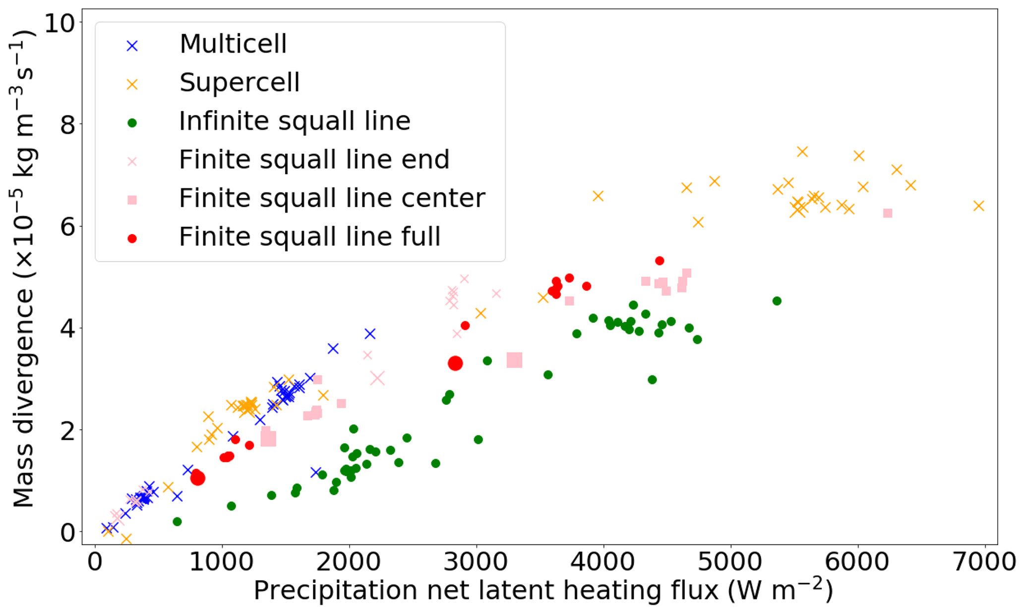
Figure 5Full dataset of upper-tropospheric mass divergence integrated over the layers 7–14 km versus net latent heating. Included are 206 records covering four modes of convection during two time intervals. The larger symbols indicate simulation data from extended-domain simulations (eight in total).
More specifically, the initial ratio between mass divergence and column latent heating is much higher for the regular multicells and supercells than for the squall lines. For increased precipitation rates, the ratio apparently decreases compared to that at low latent-heating rates. On the contrary, the same ratio for squall lines even increases with precipitation intensity, although this is not so clear. The robustness of the increment in the ratio between the mass divergence and precipitation rate of squall lines is questionable. The typically lower ratios for the supercell at high precipitation rates reduce the gap between the two regimes at higher latent-heating rates; on the one hand, there is a regime that the supercell and regular multicell seem to follow, and on the other hand, there is another regime that the (infinite-length) squall line seems to follow.
Interestingly, the physics perturbations do not substantially affect the suggested regimes, and resolution also has no noticeable effect in the plane of Fig. 5 (it should be noted that simulations with physics perturbations and a different resolution than the control runs are included in this figure). The isolated convection regime (i.e. nearly 3D outflow, applicable to regular multicells and supercells) is surprisingly linear at precipitation intensities up to about 2000 W m−2. Moreover, the contrast in the typical ratio of mass divergence and latent-heating rates (normalized mass divergence) between the two regimes that are identified is suggested to exceed a factor 2: the steep sloped line that would describe the two isolated modes of convection reaches an upper-tropospheric divergence of almost kg m−3 s−1 at 2000 W m−2, whereas only one data point for the infinite-length squall line reaches about kg m−3 s−1 at a precipitation rate of about 2000 W m−2 (≈3 mm h−1).
When one now focuses on the finite-length-squall-line simulations (pink and red symbols in Fig. 5), its end region data points (i.e. pink crosses) are in line with the mass divergence of supercell simulations. At low precipitation intensities, the mass divergence increases as rapidly as for the supercell. In addition, both supercells and end regions of finite-length squall lines have a ratio between the mass divergence and precipitation rate that reduces at higher precipitation rates in very similar ways. That decrease of the ratio between the mass divergence and precipitation rate with higher precipitation rates also occurs for central regions of the finite-length squall line (i.e. pink squares), but the mass divergence is systematically reduced compared to the end regions of the finite-length squall lines. Hence, the behaviour of the finite squall line centres aligns better with the infinite-length squall line simulations. In spite of that, the mass divergence is systematically reduced even more strongly in the infinite-length squall lines compared to the finite squall line centres.
In general, the full domain integration of the finite-length squall line leads to intermediate behaviour, with the amount of divergence in between the centre and the line end. That is a consequence of averaging over the centre and end regions. Reduced normalized mass divergence at a high precipitation intensity also occurs for the full integration over the finite-length squall lines.
Infinite-length squall lines represent nearly 2D convection (e.g. as in Moncrieff, 1992). On the other hand, initially isolated convective cells that are circular in an environment without convection follow the 3D regime (supercell and multicell). With increasing precipitation or latent-heating rates, outflows from deep convective cells are more likely to collide. They mimic idealized point or line sources less well. This effectively creates an intermediate dimensionality between 2D and 3D. The shift from or variability between purely 3D, intermediate, and purely 2D convection largely explain the variability in divergent outflows as detected. It could be seen as a non-linear effect on divergent outflow from deep convection by convective organization and aggregation. On the other hand, the absence of the effects of upscaling convective organization could have lead to a better resemblance of idealized 2D or 3D regimes.
The initial ratios between precipitation intensity and mass divergence suggest that the low precipitation intensity can obey the following two limit regimes:
-
a 2D outflow regime with reduced mass divergence
-
a 3D regime with comparatively increased mass divergence in the outflow region.
The quasi-2D regime occurs as neighbouring cells compensate for each other's divergent outflows efficiently in squall lines. Even though three-dimensional outflow from the individual cells in a squall line exists, the meridional component is largely compensated for by the neighbouring convective cells, as they also produce (opposing) meridional outflow. In the summation over the divergence of all convective cells, these meridional components compensate for and produce no net divergence along the y axis of the simulations. Therefore, the zonal component of the net divergence is 1 order of magnitude larger in an infinite-length squall line than in the meridional component (next section, Sect. 3.5). The ratio between mass divergence in the two regimes could be around a factor of 3 according to the dataset of Fig. 5. At higher precipitation intensities, these regimes are not obeyed in our simulations, as mentioned. This means that a line at intermediate normalized mass divergence between the two regimes might exist, around which all data points scatter at high precipitation intensities. In the finite-length-squall-line case, the mixed or intermediate dimensionality is already effective at low precipitation intensity. This concept and qualitative explanation connects the findings of the LES simulations with Bretherton and Smolarkiewicz (1989), Nicholls et al. (1991), and Mapes (1993).
Investigating the set of larger symbols in the scatter plot (Fig. 5) – namely those symbols that represent a supercell simulation in an extended domain – we see that they appear within the range of data points covering the perturbations. Similarly, for the finite-length-squall-line simulations, the ratio of mass divergence to net latent heating is often slightly lower than that associated with the ensemble mean. Nevertheless, divergence in extended-domain simulations is never substantially outside of the range within each mode of convection.
The ordering of the different modes of convection (with regular-multicell, supercell, and finite squall line ends inducing the most mass divergence at a given precipitation rate, followed by the full finite-length squall line, the finite-length-squall-line centre, and, lastly, the infinite-length squall line with the weakest mass divergence) is hardly affected by any of the perturbations among all the simulations (see Fig. 1 for an overview of the perturbations). That ordering indicates that the mass divergence at given precipitation rate depends on the organization of a convective system. Initially, it is suggested to manifest as a 2D outflow regime (line source) with weaker mass divergence on the one hand, while a convective 3D regime (point source) enhances mass divergence on the other hand. At high precipitation rates and over the course of time, the convective systems do not stick to these idealized regimes.
By focusing on the multicell divergences in Fig. 5, it can be induced that contrasts in the divergence relative to the precipitation between the first and second time interval do not or hardly exist. Based on this argument and upon closer inspection of the spatial distribution of divergence patterns in the simulation dataset, it is found that the precipitation (heating) pattern is solely responsible for the region of upper-tropospheric divergent flow.
3.5 Zonal and meridional divergence components in finite squall line
The existence of two outflow regimes (2D and 3D divergence) has been
-
suggested in the previous section
-
suggested by analytical expressions of flow perturbations derived from a linearized gravity wave model forced by heating (Bretherton and Smolarkiewicz, 1989; Nicholls et al., 1991; Mapes, 1993; Pandya and Durran, 1996; Nascimento and Droegemeier, 2006)
-
documented for related pressure perturbations and updraught strengths by Morrison (2016a, b).
In this section the u and v components of the upper-tropospheric divergence are separately investigated for the finite-length squall line.
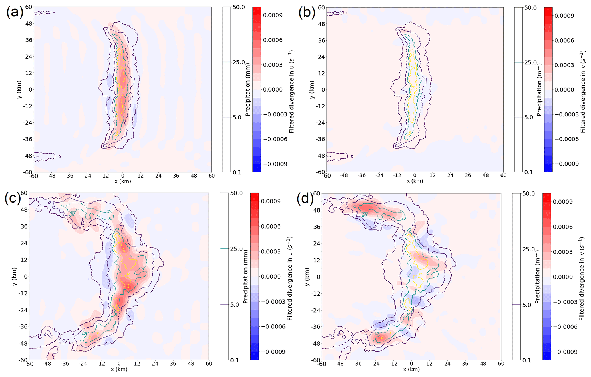
Figure 6Spatial distribution of filtered divergence over altitudes 7–14 km for a finite squall line during the (a, b) first and (c, d) second time interval. Wavelengths that fit more than 20 times in the domain have been removed with a discrete cosine transform. Contours indicate the accumulated precipitation pattern during each of the two time intervals (0.1, 5, 25, and 50 mm, as displayed in one of the two colour bars). Both the zonal (a, c) and the meridional divergence components (b, d) are displayed separately.
Figure 6a and b show that, during the initial time interval, the meridional component of the divergence is negligible throughout most of the domain. The pattern in the v term of the divergence is consistent with this part of the finite-length squall line resembling the 3D outflow regime. Similar patterns have been identified for the infinite-length squall line (not shown) but without an enhanced meridional component of divergence at the squall line end. Practically, all divergence occurs initially in the u component, which is consistent with the manifestation of a 2D-like outflow regime in the infinite-length squall line and the centre region of the finite-length squall line (Fig. 5).
During the second time interval, the v components develop particularly strongly on the northern- and southern-arching regions of the squall line. Both components are of the same order of magnitude, but that is to be expected for a strongly curved squall line. The pattern of squall line curvature is clear from the accumulated precipitation (and, similarly, the simulated radar imagery in Fig. 2l). The possibility that outflow collisions occur and that the effective flow resembles a regime governed by a mixture of 2D and 3D regimes as a result of interference between outflows from individual convective cells is strongly supported by both Figs. 5 and 6. Hence, Fig. 6 provides further evidence for the explanation of Sect. 3.4.
The (mean) divergence in Fig. 6a is about 1 order of magnitude larger than in Fig. 6b in the squall line centre. This is also consistent with the infinite-length squall line, where the difference is about 1 order of magnitude too. In the bottom panels of the figure, that contrast has strongly reduced as a result of the arching squall line, which is in accordance with expectations of bending mixed 2D–3D convection. Therefore, the leading order divergence variability in Fig. 5 can confidently be attributed to the dimensionality of outflows (2D and 3D) and, correspondingly, the presence of a pulse or line source of latent heating.
4.1 Detection of outflow: spatial and temporal analysis windows
Upper-tropospheric outflow from deep convection has been quantified for each simulation by integrating the mean mass divergence in 3D over a region surrounding the convective cells (horizontally) and over 7–14 km altitude. Figure 4 and divergence profiles (not shown) revealed that the lower boundary is the most critical of the two. Therefore, the integration has been repeated for the 6–14 km layer. The resulting patterns in a diagram of latent heating versus divergence comparable to Fig. 5 are not sensitive to the lower boundary.
The procedure has been executed for two time intervals separately: a first time interval where the fastest gravity waves escape the box of integration and a second time interval where a large proportion of the gravity wave signal has escaped that box. Even though some potentially relevant flow effects with consequences for upper-tropospheric (UT) divergence could have escaped this integration box with the gravity waves, the results suggest that this is not the case. That such an escape did not have consequences for diagnosed UT divergence can be justified with the following arguments:
-
The mechanism of gravity waves is to restore density anomalies with fluctuations, which are averaged out when integrated over longer distances in the quasi-horizontal plane.
-
The similarity of the ratio between mass divergence and net latent heating (1) during the first and second time intervals for regular multicells and (2) to supercell simulations during the first time interval suggests that an escape of gravity waves plays no role in the mass divergence. It certainly does not dilute the outflow divergence by underdetection.
-
Mass divergence of updraught outflow cannot initiate at a location outside of the convective cell's updraught itself, and spatial distributions of the winds and cumulative precipitation (e.g. Sect. 3.5) support that argument.
-
Related to the previous argument is that the testing of different integration masks for the large-domain supercell simulation indicates that mass divergence only decreases relative to the precipitation rate (!) when integrating over a too-large domain. This is a sign of a substantial increase in subsidence within the integration mask as soon as the mask is altered; the subsidence develops with gravity wave propagation (see Bretherton and Smolarkiewicz, 1989; Mapes, 1993; and the Supplement). The tests essentially suggest that the essential divergent outflows are included by including the precipitation cores within the integration mask. That is consistent with the spatial distribution of our divergence signals and with the linear gravity wave adjustment model triggered by convective heating patterns, as documented in Bretherton and Smolarkiewicz (1989) and Nicholls et al. (1991).
An integration mask covering the convective cores and ending just outside of the area of precipitation accumulation leads to the detection of a large proportion of the divergent outflows. Little dilution from convergence (i.e. inflow) may occur if appropriate vertical levels are selected for vertical integration.
4.2 Deviations of perturbed simulations from main UT divergence structure
4.2.1 Physics perturbations
In Fig. 5, one can see a very robust signal of convective organization with significance for the divergent outflow. However, a few odd data points occur. By design and nature, the strongest physical perturbations (e.g. the −40 % latent-heating constant) suppress the deep convection, and while some precipitation occurs in these perturbed simulations, the divergent outflow does not fit vertically in the integration mask – this is also the case for the ensemble and the large majority of other simulations. It is verified that data points appearing as outliers in Fig. 5 shift towards those of similar organization type if the vertical mask of divergent-outflow integration is shifted appropriately to other vertical levels (with appropriate density weighting). An extension of Fig. 4 can be found in Fig. S3 of the Supplement. The dataset visualized in this figure shows how the integration masks of outliers have to be shifted for better alignment of particular simulations with the general pattern in Fig. 5.
4.2.2 Specific role of convective momentum transport
The strong order in Fig. 5 directly suggests that convective momentum transport does not have a direct systematic impact on divergent outflow from deep convection. That does not imply that convective momentum transport does not play a role at all: it can modify the convective evolution and subsequent organization indirectly and can therefore affect the precipitation intensity. The latter two do affect the divergent outflow, as the dataset presented in Fig. 5 revealed. Even if some scatter in the mass divergence occurs for a given precipitation rate and convective organization type, it does not systematically relate to increases or decreases in convective momentum transport. Such scatter mainly occurs at high precipitation rates for the infinite-length squall line and the supercell in Fig. 5.
4.2.3 Adjusted low-level stratification
The signal of convective organization in Fig. 5 is robust. This is because the ordering of the different modes of convection is robustly present within a dataset comprising the background ensemble, physically perturbed simulations (in two ways), and the simulations on extended domains. Additionally, initial condition potential temperature profiles have been perturbed in an additional set of simulations (see Sect. 2.3.3 and Fig. 1) to test whether the stratification of the low levels has a substantial impact. The dataset obtained suggests that this is not the case. Similar perturbations have been used for the wide ensemble of finite-length squall lines. The structure in Fig. 5 is well established, and this implies that a wider range of initial conditions other than just those of a specific thermodynamic profile is explored with the dataset. The data strongly suggest that the magnitude of divergent outflow relates to net latent heating in a similar way, irrespective of the strength of near-surface inversions and the magnitude of moist instability.
4.3 Two mass divergence regimes at low precipitation rates
Figure 5 suggests that the equivalent of about 1500 W m−2 of precipitation is needed for kg m−3 s−1 of divergence at low precipitation rates in an infinite-length squall line, whereas this is only about 500 W m−2 for the regular-multicell and supercell regimes. The proportionality between these two regimes is well over a factor 2 and likely very close to 3 and π.
The idea of the finite-length-squall-line simulations is that the outer part at both of the squall line ends mimics a regime where convective cells can freely induce their outflow in a 3D space when both ends are combined (as if the centre is removed), as in the case of a multicell and supercell. The centre, however, is geometrically somewhat restricted, as in that of an infinite-length squall line. Infinite-length squall lines only allow for outflow in one horizontal direction. The idea is supported by the magnitudes of two components of the mass divergence in finite- and infinite-length squall line simulations: outflow in the zonal direction exceeds that in the meridional direction by 1 order of magnitude, which is consistent with findings pointed out by Nascimento and Droegemeier (2006). Similarly, in the finite-length squall line, divergent outflow is much larger in the direction normal to the finite-length squall line than in that parallel to the squall line initially, with dynamics induced by small cells (short wavelengths) compensating for each other in the parallel direction (Fig. 6). That provides further support for the idea of two outflow regimes.
Outflow simulations with expressions based on the numerical model of Bretherton and Smolarkiewicz (1989) and Nicholls et al. (1991) suggest that the ratio of convective outflows between a line source and point source is a factor of 2π in the limit case. That stems (in their calculations) from a conversion of the delta function from radial geometry to an x–y plane in their derivation (Nicholls et al., 1991). A mechanism that could explain the deviation of about a factor of 2 between their linear gravity wave models and large-eddy cloud simulations as performed here has not been found yet. Theoretical support for different regimes of updraught and pressure perturbations between 2D (a line source) and 3D (a point source) in a weak-shear environment is also provided by Morrison (2016a). The updraughts and pressure perturbations as studied by Morrison (2016a) drive the outflows as studied here; outflows relate to updraughts through continuity. Morrison (2016a) derived a deviation of a factor of 2 theoretically and subsequently compared the findings to cloud simulations (Morrison, 2016b).
The robustness of the results, together with the arguments above, give high confidence in the impact of outflow dimensionality on the magnitude of the divergent winds. Furthermore, the intermediate ratio of mass divergence to precipitation rate at high precipitation intensities compared to the initial 2D (low ratio) and 3D (high ratio) regimes suggests that convective aggregation likely affects the dimensionality of convective outflow in the upper troposphere. Outflow likely adapts to a mixture of 2D and 3D regimes due to the convective organization and interference between outflows of individual cells. When aggregates of convective cells collide with upper-tropospheric outflows of other convective cells, the effective dimensionality would be something intermediate between 2D and 3D: the outflows first collide along the line through the updraughts and become nearly 2D along the line, but on the outer regions, the outflow can still move as if the convective cell was isolated. That corresponds to a nearly 3D outflow regime, and any mixture creates ovals of outflow similar to the finite squall line in our conceptual framework (even if the supercells also reveal such behaviour and collisions of outflow after some time).
4.4 Implications and future research
The mass divergence found in the dataset (Fig. 5) is, in terms of magnitude, in good agreement with linear gravity wave adjustment models where heating is imposed as proxy for a convective system (Bretherton and Smolarkiewicz, 1989; Nicholls et al., 1991; Mapes, 1993; Pandya et al., 1993; Pandya and Durran, 1996).
The initial 2D and 3D regime behaviour with reduced divergence at higher precipitation intensities due to convective aggregation found in this study contrasts with the modelling and observation studies by Mapes (1993) and Mapes and Houze (1995). In Mapes (1993), it is suggested that a stratiform contribution by the vertical half wavelength due to a stratiform fraction of a mesoscale convection system actually increases the divergence at any given heating rate or at a given precipitation intensity. On the one hand, this could imply that the convective systems simulated in this study do not extend sufficiently and so do not generate any sizeable stratiform precipitation system. Indeed, the stratiform contribution to the simulated squall line and supercell clouds is not substantial, especially when looking at the precipitation that reaches the surface (turned into net latent heating); see Figs. 2 and S1 in the Supplement (see also Groot and Tost, 2023). The formation of a stratiform precipitation regime usually coincides with lifting of the level of neutral divergence, on average (Mapes, 1993; Houze, 2004). In Fig. 4, such a continuous gradual rising of the level of neutral divergence for supercells and squall lines during the second hour cannot be detected. However, at least a fraction of an MCS is usually stratiform within the second hour. This suggests that the simulations are only representative for purely convective systems or for those with minor stratiform fractions, which is a reasonable approximation to convection in certain regions (Schumacher et al., 2004). In spite of this, these purely convective systems are important to study for a better understanding of the role of deep convection in the climate system and to improve deep-convective parameterizations.
On the contrary, using Fig. 5, one could argue that a stronger increase of the mass divergence with latent-heating rate occurs for the infinite-length-squall-line simulations at rather high latent-heating rates rather than at low latent-heating rates (as the highest latent-heating rates occur in the second hour). Furthermore, stratiform precipitation systems may form out of the squall line anvils. That would be in agreement with arguments by Mapes (1993) and Mapes and Houze (1995), assuming that the stratiform fraction of the system increases with time. However, an infinite-length squall line is, in practice, not very representative for most deep convection in the real world. In addition, the level of neutral divergence does not seem to rise at all for the infinite-length squall line in Fig. 4, which would not support possible compatibility of our results with the arguments of Mapes (1993) and Mapes and Houze (1995). Furthermore, the more realistic finite-length squall line does not behave in agreement with these studies. In the finite-length squall lines, the ratio between the mass divergence and net latent heating decreases at higher precipitation rates during the second (later) time interval (Fig. 5).
Theoretical 2D squall line models have been extensively studied by Moncrieff and co-authors (e.g. Moncrieff, 1992). In Moncrieff (1992), it was argued that such 2D models could be very beneficial for parameterizing convective momentum transport. Trier et al. (1997) pointed out that one should be careful and that processes such as convective momentum transport in actual squall line convection can have characteristics of a mixture of 2D and 3D convection. Certain sections have more characteristics of a 2D convection regime, and others have more characteristics of a 3D convection regime. The finite squall lines suggest that the same is true regarding divergence profiles. That means that a comparison of traditional and theoretical models of idealized convection (e.g. 2D models) to cloud-resolving and large-eddy simulations is needed. By stimulating such model intercomparisons, the applicability of traditional practices and findings to the more complex simulation techniques can be scrutinized (as done here and in Morrison, 2016a, b).
Theoretically, convectively induced divergence profiles are suggested to mimic 2D or 3D regimes in some cases. On the contrary, in practice, intermediate behaviour is suggested to be more likely, especially for intensive systems. That can be a worthwhile consideration for the development of convective parameterizations that would take convective organization and aggregation into account (e.g. Moncrieff, 2019).
In Baumgart et al. (2019) and Zhang et al. (2007), it was found that numerical weather prediction errors are initially established predominantly in regions of enhanced and mostly convective precipitation. Baumgart et al. (2019) were able to attribute initial error growth (<12 h into the simulation) in their stochastically perturbed simulations to non-conservative processes and predominantly to the deep-convection parameterization. That parameterization represents the collective effect of organized convective systems and isolated convective cells. At later times, the induced ensemble variability corresponds predominantly to variability in upper-tropospheric divergent winds. Baumgart et al. (2019) inferred that this upper-tropospheric variability is likely associated with latent-heat release below and corresponding deep convection as precursors.
The quantitative understanding of upper-tropospheric outflow and the uncertainty quantification achieved in this work could support an extension of the potential vorticity diagnostics of Baumgart et al. (2019) towards smaller scales. Consequently, it may lead to better insights into the role of individual convective systems in certain forecast errors. Furthermore, it may reveal biases between certain modelling approaches, namely large-eddy simulation, cloud-resolving simulations with explicit deep convection, and global simulations with parameterized deep convection (see for example Done et al., 2006). Intercomparison of divergent outflows among the simulations investigated here and various simulation set-ups could provide structural insights into (potential) biases between each of them. Such insights into structural biases depending on the treatment of deep convection may be beneficial to the understanding of weather and climate simulations. In this work, a set-up for the intercomparison of divergent outflows is established, focusing on large-eddy simulations with advanced small-scale-process representation. The effects of differential convective organization or differential diabatic heating could potentially be followed to synoptic-scale uncertainty days ahead using a thorough understanding of upper-tropospheric divergence variability (e.g. Baumgart et al., 2019; Rodwell et al., 2013). This study builds the insights into which main factors control the upper-tropospheric divergence, which is required to trace mesoscale uncertainty induced by diabatic heating, while its uncertainty can evolve upscale to synoptic-scale uncertainty.
LES simulations of four types of convection with ensemble, physics, resolution, and other modifications have shown that upper-tropospheric mass divergence associated with deep convective systems depends on net latent heating (i.e. precipitation intensity) and on the convective organization. Divergent outflows have been integrated over a fixed area and 7–14 km altitude. Thereby, the main precipitation cores for each type of convection have been covered and split over two time intervals (Fig. 3). Wind profiles were imposed such that the convective cells propagate slowly with respect to the domain, and therefore their flow perturbation accumulated in a condensed region. The relation between mean mass divergence and net-latent-heating rates has been analysed and intensively discussed. At low precipitation rates and in initial development stages, the four basic scenarios strongly suggest the existence of a 3D outflow regime for isolated convective cells (i.e. supercell and regular multicell). On the other hand, a 2D outflow regime exists, as demonstrated by the infinite-length squall line. Within each regime, a linear dependence of mass divergence on net latent heating is found. In practice, a more realistic squall line is suggested to conform to a mixture of the 2D and 3D regimes. At higher precipitation intensities, the outflow does not strictly follow these two regimes anymore. The magnitude of the mass divergence associated with high net-latent-heating rates is somewhat intermediate between the initial 2D and 3D regimes, but ordering between different organizational types of convection still occurs at high net-latent-heating rates. Given an outflow dimensionality, UT divergent convective outflow therefore depends linearly on net latent heating accordingly. This dependence is the key finding of this study. Additionally, non-linear dependence occurs through convective aggregation and organization that can modulate outflow dimensionality.
Simulations on extended domains, in addition to an ensemble of simulations, strengthen the confidence in the results. Convective momentum transport plays no direct role in the mass divergence in the simulations. Nevertheless, by affecting the organization and precipitation rates within a convective system, it can indirectly affect upper-tropospheric mass divergence.
An important implication of this study is a potential bias in upper-tropospheric divergent flow if the convective organization is unknown or misrepresented (as is generally the case for parameterization). This implication would exist even if the precipitation rate or some kind of statistical distribution describing the spatial mean and variability of the precipitation rate were known.
The findings are in good agreement with the linear gravity wave adjustment models triggered by convective heating in Bretherton and Smolarkiewicz (1989), Nicholls et al. (1991), Mapes (1993), and Morrison (2016a, b) if we assume a purely convective heating regime. However, the simulations of this study do not reveal any substantial heating contributions from stratiform fractions of mesoscale convection (Mapes, 1993). Therefore, anything specific regarding the role of vertical modes other than that of the basic convective-heating profile triggering wavelength 2H (twice the depth of the troposphere) cannot be concluded. Additional simulations beyond the scope of this study would be necessary to understand the role of secondary gravity wave modes affecting UT divergence. Simulations tackling the effect of those modes would have to be focused on the finite- and infinite-length squall lines at larger domains specifically. Longer integrations are needed to inspect the effect of those modes.
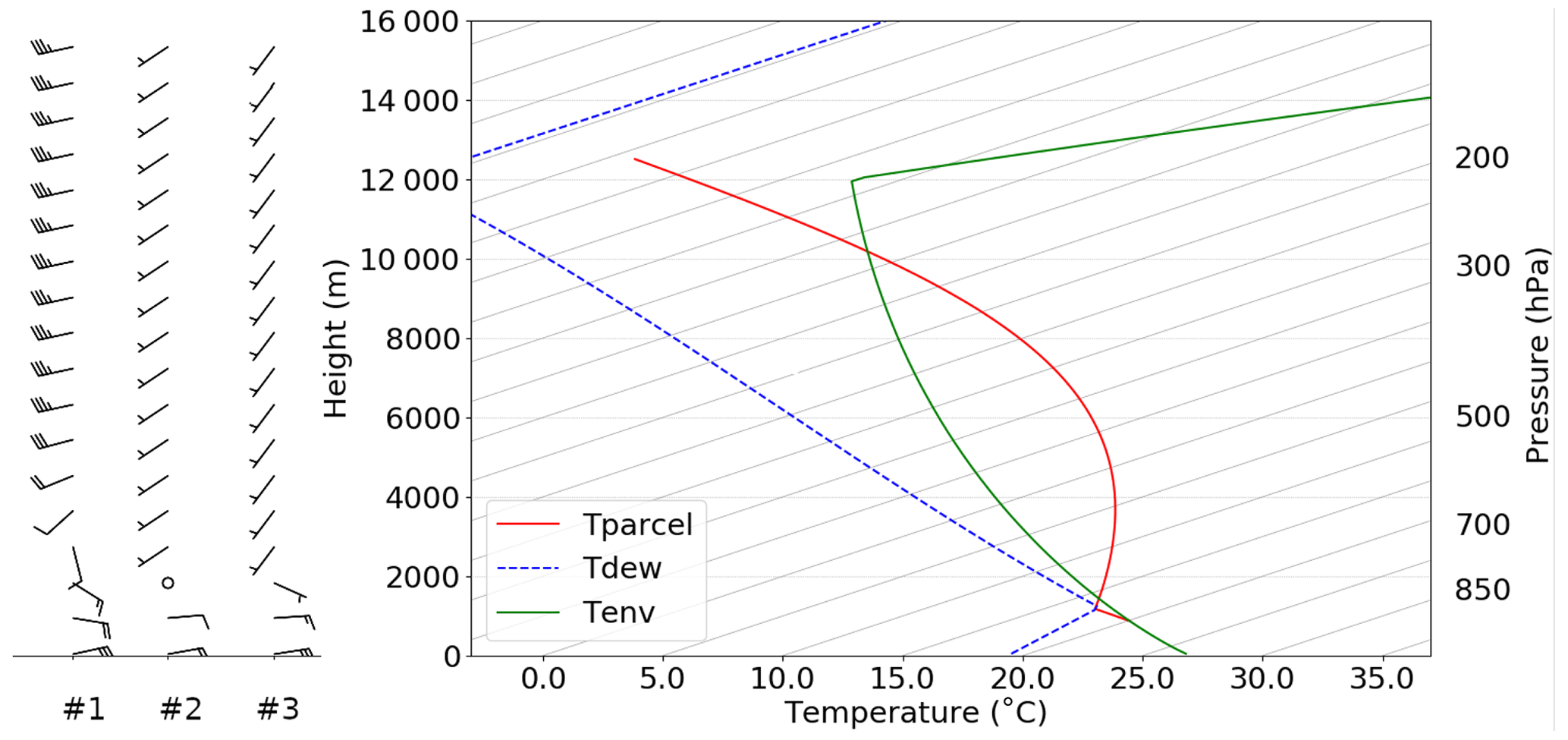
Figure A1Temperature and moisture profile following Weisman and Klemp (1982) and wind profiles 1–3 (left). Temperature: solid green line; dew point: dashed blue line; temperature of parcels when lifted from about 900 m altitude (no dilution): red line.
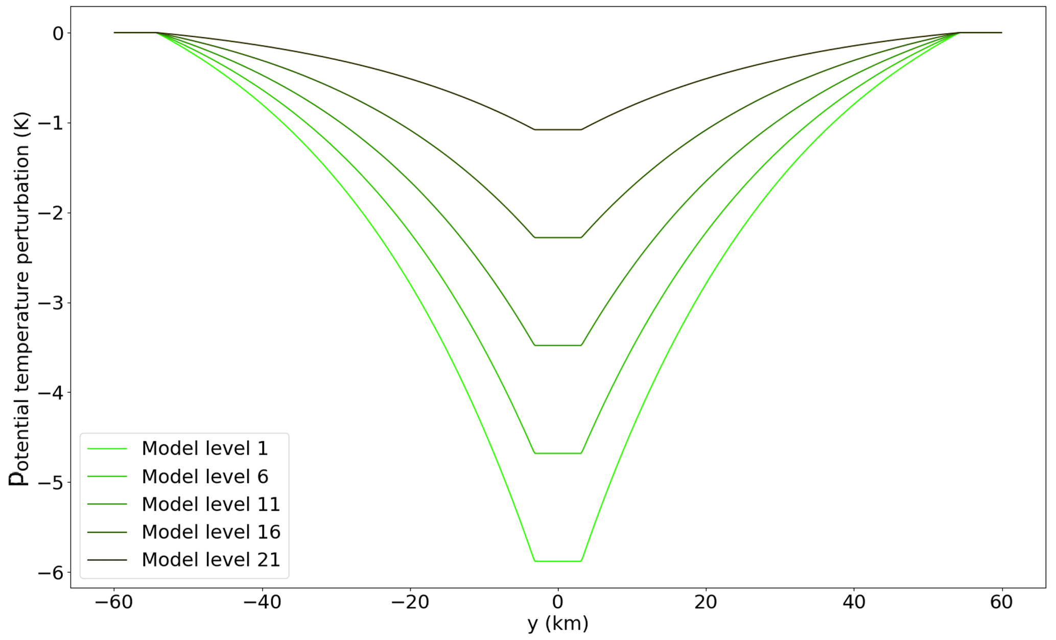
Figure A2North–south profile of initial potential temperature perturbations along the length of the finite-length squall line for five selected model levels, counted upwards from the surface level.
Parts of the output of this study are available for download at https://doi.org/10.5281/zenodo.6619313 (Groot, 2022) (accompanying dataset of Groot and Tost, 2023; last access: 10 January 2023), and other parts are available at https://doi.org/10.5281/zenodo.7629669 (Groot, 2023). A download script and README file are provided there.
The code in the “Code availability” statement, together with the Supplement, allows readers to download our data from this work (https://doi.org/10.5281/zenodo.6619313, Groot, 2022; https://doi.org/10.5281/zenodo.7629669 Groot, 2023; Supplement).
The supplement related to this article is available online at: https://doi.org/10.5194/acp-23-6065-2023-supplement.
The idea for this study originates from the authors in collaboration with colleagues from TRR 165. The study was designed, conducted, and composed by EG, with contributions from and under the supervision of HT.
At least one of the (co-)authors is a member of the editorial board of Atmospheric Chemistry and Physics. The peer-review process was guided by an independent editor, and the authors also have no other competing interests to declare.
Publisher's note: Copernicus Publications remains neutral with regard to jurisdictional claims in published maps and institutional affiliations.
The authors would like to thank the collaborators in the Waves to Weather project A1, namely George Craig, Michael Riemer, and Tobias Selz, for their input and, in addition, those who helped the lead author facilitate the initialization of CM1 on the high-performance computer in Mainz, namely Manuel Baumgartner (now at DWD) and Christopher Polster. Lastly, we would like to thank the reviewers for their useful suggestions and the editor for handling the paper.
The authors would also like to acknowledge the computing time granted on the supercomputer MOGON 2 at Johannes Gutenberg-University Mainz (https://hpc.uni-mainz.de, last access: 10 January 2023).
This research has been supported by the Deutsche Forschungsgemeinschaft (grant no. TRR-165). Holger Tost received
additional funding from the Carl Zeiss foundation.
This open-access publication was funded by Johannes Gutenberg University Mainz.
This paper was edited by Thijs Heus and reviewed by two anonymous referees.
Baumgart, M., Ghinassi, P., Wirth, V., Selz, T., Craig, G. C., and Riemer, M.: Quantitative View on the Processes Governing the Upscale Error Growth up to the Planetary Scale Using a Stochastic Convection Scheme, Mon. Weather Rev., 147, 1713–1731, https://doi.org/10.1175/mwr-d-18-0292.1, 2019. a, b, c, d, e, f
Bierdel, L., Selz, T., and Craig, G.: Theoretical aspects of upscale error growth through the mesoscales: an analytical model, Q. J. Roy. Meteor. Soc., 143, 3048–3059, https://doi.org/10.1002/qj.3160, 2017. a, b
Bierdel, L., Selz, T., and Craig, G. C.: Theoretical aspects of upscale error growth on the mesoscales: Idealized numerical simulations, Q. J. Roy. Meteor. Soc., 144, 682–694, https://doi.org/10.1002/qj.3236, 2018. a, b
Bretherton, C. S. and Smolarkiewicz, P. K.: Gravity Waves, Compensating Subsidence and Detrainment around Cumulus Clouds, J. Atmos. Sci., 46, 740–759, https://doi.org/10.1175/1520-0469(1989)046<0740:GWCSAD>2.0.CO;2, 1989. a, b, c, d, e, f, g, h, i, j, k, l
Bryan, G.: Cloud Model 1, Version 19.8/cm1r19.8, NCAR [code], https://www2.mmm.ucar.edu/people/bryan/cm1/ (last access: 10 January 2023), 2019. a, b
Bryan, G. H., Wyngaard, J. C., and Fritsch, M. J.: Resolution Requirements for the Simulation of Deep Moist Convection, Mon. Weather Rev., 131, 2394–2416, 2003. a
Clarke, S. J., Gray, S. L., and Roberts, N. M.: Downstream influence of mesoscale convective systems. Part 1: influence on forecast evolution, Q. J. Roy. Meteor. Soc., 145, 2933–2952, https://doi.org/10.1002/qj.3593, 2019a. a
Clarke, S. J., Gray, S. L., and Roberts, N. M.: Downstream influence of mesoscale convective systems. Part 2: Influence on ensemble forecast skill and spread, Q. J. Roy. Meteor. Soc., 145, 2953–2972, https://doi.org/10.1002/qj.3613, 2019b. a
Deardorff, J. W.: Stratocumulus-capped mixed layers derived from a three-dimensional model, Bound.-Lay. Meteorol., 18, 495–527, https://doi.org/10.1007/bf00119502, 1980. a
Done, J. M., Craig, G. C., Gray, S. L., Clark, P. A., and Gray, M. E. B.: Mesoscale simulations of organized convection: Importance of convective equilibrium, Q. J. Roy. Meteor. Soc., 132, 737–756, https://doi.org/10.1256/qj.04.84, 2006. a
Grant, L. D., P., L. T., and van den Heever, S. C.: The role of cold pools in tropical oceanic convective systems, J. Atmos. Sci., 75, 2615–2634, https://doi.org/10.1175/jas-d-17-0352.1, 2018. a
Groot, E.: Output data and namelist – README file “Evolution of squall line variability and error growth in an ensemble of LES”, Zenodo [code and data set], https://doi.org/10.5281/zenodo.6619313, 2022. a, b
Groot, E.: Dataset of “Divergent convective outflow in large eddy simulations”, Zenodo [code and data set], https://doi.org/10.5281/zenodo.7629669, 2023. a, b
Groot, E. and Tost, H.: Evolution of squall line variability and error growth in an ensemble of large eddy simulations, Atmos. Chem. Phys., 23, 565–585, https://doi.org/10.5194/acp-23-565-2023, 2023. a, b, c, d, e, f
Houze, R. A.: Mesoscale convective systems, Rev. Geophys., 42, RG4003, https://doi.org/10.1029/2004rg000150, 2004. a, b
Houze, R. A.: 100 Years of Research on Mesoscale Convective Systems, Meteor. Mon., 59, 17.1–17.54, https://doi.org/10.1175/AMSMONOGRAPHS-D-18-0001.1, 2018. a
Lane, T. P. and Reeder, M. J.: Convectively Generated Gravity Waves and Their Effect on the Cloud Environment, J. Atmos. Sci., 58, 2427–2440, https://doi.org/10.1175/1520-0469(2001)058<2427:CGGWAT>2.0.CO;2, 2001. a
Lane, T. P. and Zhang, F.: Coupling between gravity waves and tropical convection at Mesoscales, J. Atmos. Sci, 68, 2582–2598, https://doi.org/10.1175/2011JAS3577.1, 2011. a
Mapes, B. E.: Gregarious Tropical Convection, J. Atmos. Sci., 50, 2026–2037, https://doi.org/10.1175/1520-0469(1993)050<2026:GTC>2.0.CO;2, 1993. a, b, c, d, e, f, g, h, i, j, k, l
Mapes, B. E. and Houze, R. A.: Diabatic Divergence Profiles in Western Pacific Mesoscale Convective Systems, J. Atmos. Sci., 52, 1807–1828, https://doi.org/10.1175/1520-0469(1995)052<1807:DDPIWP>2.0.CO;2, 1995. a, b, c
Moncrieff, M. W.: Organized Convective Systems: Archetypal Dynamical Models, Mass and Momentum Flux Theory, and Parametrization, Q. J. Roy. Meteor. Soc., 118, 819–850, https://doi.org/10.1002/qj.49711850703, 1992. a, b, c
Moncrieff, M. W.: Toward a dynamical foundation for organized convection parameterization in GCMs, Geophys. Res. Lett., 46, 14103–14108, 2019. a
Morrison, H.: Impacts of Updraft Size and Dimensionality on the Perturbation Pressure and Vertical Velocity in Cumulus Convection. Part I: Simple, Generalized Analytic Solutions, J. Atmos. Sci., 73, 1441–1454, https://doi.org/10.1175/JAS-D-15-0040.1, 2016a. a, b, c, d, e, f
Morrison, H.: Impacts of Updraft Size and Dimensionality on the Perturbation Pressure and Vertical Velocity in Cumulus Convection. Part II: Comparison of Theoretical and Numerical Solutions and Fully Dynamical Simulations, J. Atmos. Sci., 73, 1455–1480, https://doi.org/10.1175/JAS-D-15-0041.1, 2016b. a, b, c, d
Morrison, H., Thompson, G., and Tatarskii, V.: Impact of Cloud Microphysics on the Development of Trailing Stratiform Precipitation in a Simulated Squall Line: Comparison of One- and Two-Moment Schemes, Mon. Weather Rev., 137, 991–1007, https://doi.org/10.1175/2008mwr2556.1, 2009. a
Nascimento, E. L. and Droegemeier, K. K.: Dynamic Adjustment in a Numerically Simulated Mesoscale Convective System: Impact of the Velocity Field, J. Atmos. Sci., 63, 2246–2268, https://doi.org/10.1175/JAS3744.1, 2006. a, b
Nicholls, M. E., Pielke, R. A., and Cotton, W. R.: Thermally Forced Gravity Waves in an Atmosphere at Rest, J. Atmos. Sci., 48, 1869–1884, https://doi.org/10.1175/1520-0469(1991)048<1869:TFGWIA>2.0.CO;2, 1991. a, b, c, d, e, f, g, h
Pandya, R., Durran, D., and Bretherton, C.: Comments on “Thermally Forced Gravity Waves in an Atmosphere at Rest”, J. Atmos. Sci., 50, 4097–4101, 1993. a, b
Pandya, R. E. and Durran, D. R.: The influence of convectively generated thermal forcing on the mesoscale circulation around squall lines, J. Atmos. Sci., 53, 2924–2951, https://doi.org/10.1175/1520-0469(1996)053<2924:TIOCGT>2.0.CO;2, 1996. a, b, c
Rodwell, M. J., Magnusson, L., Bauer, P., Bechtold, P., Bonavita, M., Cardinali, C., Diamantakis, M., Earnshaw, P., Garcia-Mendez, A., Isaksen, L., Källén, E., Klocke, D., Lopez, P., McNally, T., Persson, A., Prates, F., and Wedi, N.: Characteristics of Occasional Poor Medium-Range Weather Forecasts for Europe, B. Am. Meteorol. Soc., 94, 1393–1405, https://doi.org/10.1175/bams-d-12-00099.1, 2013. a, b, c
Rotunno, R., Klemp, J. B., and Weisman, M. L.: A theory for strong, long-lived squall lines, J. Atmos. Sci., 45, 463–485, https://doi.org/10.1175/1520-0469(1988)045<0463:ATFSLL>2.0.CO;2, 1988. a, b, c
Schumacher, C., Houze, R. A., and Kraucunas, I.: The Tropical Dynamical Response to Latent Heating Estimates Derived from the TRMM Precipitation Radar, J. Atmos. Sci., 61, 1341–1358, https://doi.org/10.1175/1520-0469(2004)061<1341:TTDRTL>2.0.CO;2, 2004. a
Stechmann, S. N. and Majda, A. J.: Gravity waves in shear and implications for organized convection, J. Atmos. Sci, 66, 2579–2599, https://doi.org/10.1175/2009JAS2976.1, 2009. a
Trier, S. B., Skamarock, W. C., and LeMone, M. A.: Structure and Evolution of the 22 February 1993 TOGA COARE Squall Line: Organization Mechanisms Inferred from Numerical Simulation, J. Atmos. Sci., 54, 386–407, https://doi.org/10.1175/1520-0469(1997)054<0386:SAEOTF>2.0.CO;2, 1997. a
Weisman, M. L. and Klemp, J. B.: The Dependence of Numerically Simulated Convective Storms on Vertical Wind Shear and Buoyancy, Mon. Weather Rev., 110, 504–520, https://doi.org/10.1175/1520-0493(1982)110<0504:tdonsc>2.0.co;2, 1982. a, b, c, d, e
Zhang, F., Bei, N., Rotunno, R., Snyder, C., and Epifanio, C. C.: Mesoscale Predictability of Moist Baroclinic Waves: Convection-Permitting Experiments and Multistage Error Growth Dynamics, J. Atmos. Sci., 64, 3579–3594, https://doi.org/10.1175/jas4028.1, 2007. a