the Creative Commons Attribution 4.0 License.
the Creative Commons Attribution 4.0 License.
 | 30 May 2023
Coupled mesoscale–microscale modeling of air quality in a polluted city using WRF-LES-Chem
Domingo Muñoz-Esparza
Jianing Dai
Cathy Wing Yi Li
Pablo Lichtig
Roy Chun-Wang Tsang
Chun-Ho Liu
Guy Pierre Brasseur
To perform realistic high-resolution air quality modeling in a polluted urban area, the Weather Research and Forecasting (WRF) model is used with an embedded large-eddy simulation (LES) module and online chemistry. As an illustration, a numerical experiment is conducted in the megacity of Hong Kong, which is characterized by multi-type inhomogeneous pollution sources and complex topography. The results from the multi-resolution simulations at mesoscale and LES scales are evaluated by comparing them with ozone sounding profiles and surface observations. The comparisons show that both mesoscale and LES simulations reproduce the mean concentrations of the chemical species and their diurnal variations at the background stations well. However, the mesoscale simulations largely underestimate the NOx concentrations and overestimate O3 at the roadside stations due to the coarse representation of the traffic emissions. The LES simulations improve the agreement with the measurements near the road traffic, and the LES with the highest spatial resolution (33.3 m) provides the best results. The large-eddy simulations show more detailed structures in the spatial distributions of chemical species than the mesoscale simulations, highlighting the capability of LES to resolve high-resolution photochemical transformations in urban areas. Compared to the mesoscale model results, the LES simulations show similar evolutions in the profiles of the chemical species as a function of the boundary layer development over a diurnal cycle.
- Article
(16501 KB) - Full-text XML
-
Supplement
(1118 KB) - BibTeX
- EndNote


Air pollution represents one of the most important factors affecting human health (WHO, 2013). Human exposure to outdoor air pollution often occurs at the street level in urban canyons, and high-resolution air quality forecasting is therefore required to take appropriate preventive actions and limit air pollution (Barzyk et al., 2015; Sauer and Muñoz-Esparza, 2020). Air quality at the street level is difficult to simulate, especially if the model resolution is too coarse to properly resolve urban flows. The complexities in the distribution and variation of the chemical species in the urban canopy are due to several factors. First, the heterogeneous emissions, such as vehicle emissions at the street level, are difficult to represent in coarse models. Second, the dispersion of chemical species in turbulent flows cannot be adequately resolved by mesoscale models. Additionally, the nonlinear turbulence–chemistry interactions in the turbulent planetary boundary layer (PBL), which can be important under polluted situations, are ignored in the coarse models (Li et al., 2021; Wang et al., 2021, 2022).
Because air pollution is determined by both local dynamical circulations and long-distance transport, the accurate simulation of the species' distribution requires that mesoscale and microscale processes be coupled. Regional models, which adopt global or coarser regional model output as initial and boundary conditions, are usually applied at the spatial resolution of several kilometers, with the effects of turbulent motions being parameterized through commonly used one-dimensional PBL schemes. Mesoscale models can therefore reproduce regional-scale air pollution but are not adequate for simulating the distribution of physical and chemical variables at the urban neighborhood scale, which requires that the model resolution be less than 1 km. Moreover, the representation of air pollution near road traffic requires further increasing of the model resolution to be smaller than 40 m (Batterman et al., 2014). In order to explicitly resolve buildings in the models to fully account for the urban effects, the grid spacing should further be increased to at least 10 m (Maronga et al., 2019).
Different downscaling methods are used to represent detailed air pollution distributions in urban or industrial areas. Due to their high computational efficiency, models based on a Gaussian-type redistribution of the wind flow (Forehead and Huynh, 2018) are often adopted to represent chemical species in street canyons. However, these types of models do not directly calculate dynamical and thermal processes and ignore therefore turbulence–chemistry interactions. To better predict the nonlinear photochemical reactions in the PBL over complex underlying surfaces, the turbulent eddies need to be explicitly resolved.
There are three main basic approaches can be used to account for the effects of turbulence on the chemical species: the Reynolds-averaged Navier–Stokes (RANS) formulation, the large-eddy simulation (LES) approach, and the direct numerical simulation (DNS) method. Among these models, RANS requires the least computational resources but can only resolve the mean flows and averages out the turbulent fluctuations, while DNS directly resolves all the scales of the eddies without any approximation or parameterization; however, this approach is computationally expensive. LES, which is an intermediate approach between RANS and DNS, is a more common choice, in which the large eddies that contain most of the turbulent energy and are responsible for most of the momentum transfer and turbulent mixing are explicitly resolved, while the small eddies are parameterized using subgrid scale (SGS) schemes (Smagorinsky, 1963; Deardorff, 1970).
Computational fluid dynamics (CFD) models resolve turbulence using RANS, LES, or DNS to solve engineering problems involving fluid flows. These models are being applied more and more often to address urban pollution problems, which has become possible with the availability of large computational resources. The advantage of the CFD approach is that it can resolve the urban morphology (e.g., terrain, buildings, streets) and thus explicitly calculate the eddies across the streets and around the buildings. Such models represent the effects of the urban canopy on the dynamics of flows. They also simulate pollutant retention at street level, typically at a resolution of meters; however, their domain is usually limited to a few kilometers squared (Tominaga and Stathopoulos, 2013; Zhong et al., 2016). Many studies coupled mesoscale models with CFD models to investigate micro-scale processes in realistic applications (Baik et al., 2009; Zheng et al., 2015). However, due to the large gap between scales in mesoscale and CFD formulations, the processes covering intermediate scales are missing. In addition, CFD modules mainly focus on dynamical processes in the flow field but do not describe other major atmospheric processes related to physics, thermodynamics, radiative transfer, cloud processes, land surface exchanges, etc.
LES formulations on the other hand can also be applied in meteorological models with full physical and chemical processes in a spatial domain that is considerably larger than a common CFD domain. An illustrative example (Khan et al., 2021) of an LES module with atmospheric chemistry linked to regional information is provided by the Parallelized Large-eddy Simulation Model (PALM) for urban applications (PALM-4U) applied to an urban environment. To perform realistic studies, the PALM model uses additional tools (e.g., INIFOR, Maronga et al., 2020; WRF4PALM, Lin et al., 2021) to create initial and boundary meteorological conditions from mesoscale models. Recently, efforts by the atmospheric LES community to model urban effects have focused on exploiting the accelerated computing from GPUs (Muñoz-Esparza et al., 2020, 2021; Sauer and Muñoz-Esparza, 2020), since these fine-scale simulations are otherwise computationally too expensive.
The Weather Research and Forecasting (WRF; https://www2.mmm.ucar.edu/wrf/users/, last access: 23 May 2023; Skamarock et al., 2019) model allows multiscale nested simulations of the atmosphere with a full suite of atmospheric dynamics, surface exchanges, radiation, and cloud physics. An LES module was embedded into WRF (WRF-LES), which can be applied in two modes: (1) without external forcing from the mesoscale model or by real-world meteorological data (Moeng et al., 2007; Yamaguchi and Feingold, 2012) or (2) by being coupled with the mesoscale WRF (Nozawa and Tamura, 2012; Muñoz-Esparza et al., 2017). The WRF model can also account for atmospheric chemistry (WRF-Chem; https://ruc.noaa.gov/wrf/wrf-chem/, last access: 23 May 2023; Grell et al., 2005) and specifically simulate the transport and chemical reactions between various species with different mechanisms. In this work, we use the WRF model framework with the LES mode and online chemistry (WRF-LES-Chem) to perform multiscale simulations of atmospheric chemical species. The advantage of using WRF-LES-Chem is that all the physical and chemical processes are consistent among the different scales. This allows us to analyze the differences induced by turbulent interactions. Previous studies using coupled WRF-LES-Chem model investigated passive tracer dispersion in urban environments (Nottrott et al., 2014; Gaudet et al., 2017). Here we use a more comprehensive chemical mechanism in the coupled WRF-LES-Chem model to study the ozone photochemistry in a complex terrain.
The model experiments were conducted for the city of Hong Kong, a highly urbanized area with severe air pollution. The region is characterized by heterogeneous land use with forest over the mountains and dense constructions along the coast. The pollution originates from different sources including road transport, navigation, civil aviation, power plants, industry, hill fires, and other combustion and non-combustion emissions. The complex topography, land surface, and diverse emissions make it difficult to predict the air quality patterns and variability in the city, especially in the dense built-up area. Hong Kong therefore poses challenging questions that can be investigated with a high-resolution model and offers a perfect scenario to evaluate the capability of WRF-LES-Chem to perform high-resolution air pollution predictions.
The purpose of this work is to exploit the WRF framework with embedded LES and chemistry modules to conduct realistic high-resolution air quality simulations in a densely populated urban area. The model setup is presented in Sect. 2. The description of the observations can be found in Sect. 3. In Sect. 4, the performance of the WRF-LES-Chem model is evaluated by comparison to available observations. The influence of spatial resolution on the model results is also presented, including the impact of the resolved turbulence on atmospheric chemistry by comparing it to mesoscale model output with PBL parameterization. Section 5 summarizes the study and provides conclusions.
2.1 Dynamic settings
The WRF model coupled with chemistry (version 4.0.2) is used in the present study. The coupled mesoscale and LES module within WRF are adopted to represent spatial and temporal scales specifically capturing synoptic to turbulent motions. The model setup consists of seven one-way nested domains, out of which D01–D04 are mesoscale domains and D05–D07 are LES domains (Fig. 1). The horizontal resolutions for the mesoscale domains are 24.3 km, 8.1 km, 2.7 km, and 900 m, respectively, from the outer to inner domains, with the number of points in the zonal and meridional directions of , and 180×180 in the corresponding domains. The grid spacings in the LES domains are 300, 100, and 33.3 m, respectively, for D05 to D07, and the corresponding grid numbers are , and 243×243. The vertical layers are set to 63 levels for all the domains, with the finest vertical resolution of 12.5 to 50 m in the lowest 1.3 km (30 layers). For the heights above 1.3 km, the vertical spacing increases gradually towards the model top located at 50 hPa.
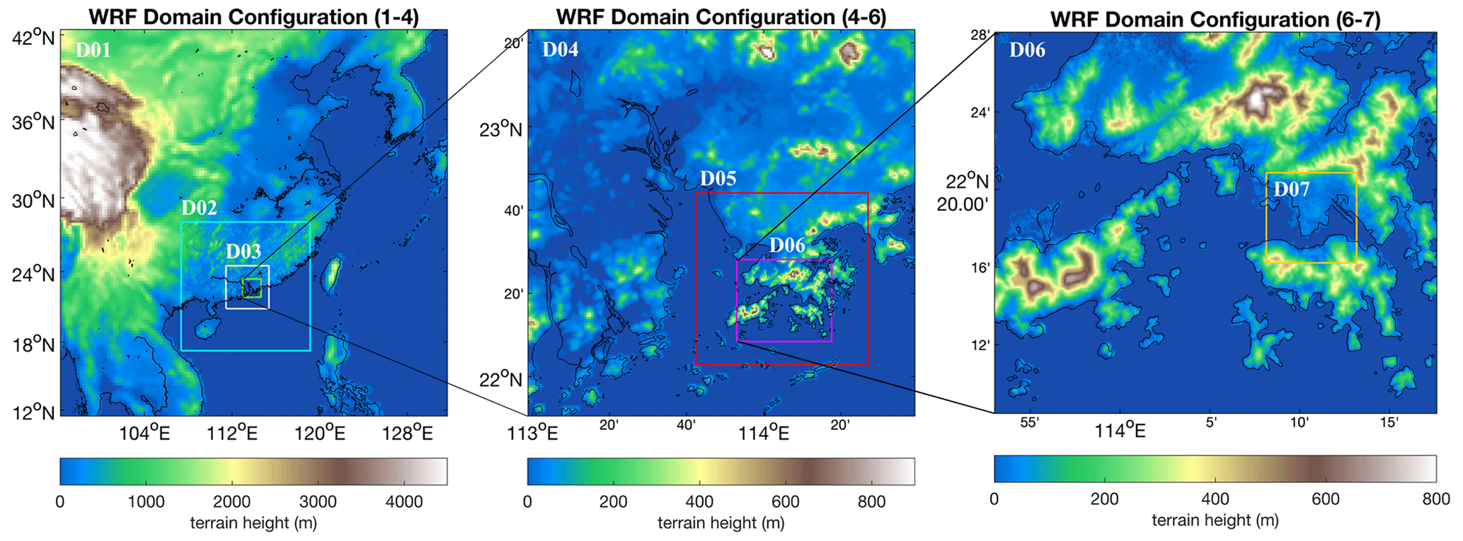
Figure 1Setup of the seven one-way nested WRF domains and a representation of the topography adopted in the model.
The meteorological initial and boundary conditions are obtained from the Final Operational Global Analysis (FNL) data produced by the National Centers for Environmental Prediction (NCEP) on 1∘ × 1∘ grids and 6 h intervals. The topography data for D01–D05 are from the Global Multi-resolution Terrain Elevation Data (GMTED2010) 30 arcsec dataset developed by the U.S. Geological Survey (USGS) and the National Geospatial-Intelligence Agency (NGA). For the two innermost domains D06 and D07, the terrain heights are adopted from the ALOS world 3D data (Takaku et al., 2014) distributed by OpenTopography (https://opentopography.org, last access: 1 June 2020) with a spatial resolution of 30 m. The topography maps after pre-processing are shown for different domains in Fig. 1. The land use data are obtained from the Noah-modified 21-category Moderate Resolution Imaging Spectroradiometer (MODIS) database developed by International Geosphere–Biosphere Programme (IGBP) at 30 arcsec resolution (Friedl et al., 2010).
The Yonsei University (YSU; Hong et al., 2006) PBL scheme is adopted in the mesoscale domains to parameterize the SGS turbulent fluxes within the PBL. The PBL parameterization, however, is turned off in the LES domains, where the large eddies are directly resolved and the effects of the small eddies are expressed by the three-dimensional 1.5-order turbulent kinetic energy (TKE) subgrid closure of Deardorff (Deardorff, 1970; Moeng, 1984). Most of the other main physical parameterizations are identical for both mesoscale and LES domains. They include the rapid radiative transfer model (RRTM) longwave radiation scheme (Mlawer et al., 1997), the Goddard shortwave radiation scheme (Chou and Suarez, 1994), the Lin microphysics scheme (Lin et al., 1983), the Noah land surface model (Chen and Dudhia, 2001), and the revised MM5 Monin–Obukhov surface layer scheme (Jiménez et al., 2012). For the coarser mesoscale simulations (D01-D03), the Grell–Freitas cumulus scheme (Grell and Freitas, 2014) is used, while it is turned off in the innermost mesoscale domain (D04) and the LES domains. The urban canopy scheme is turned off in both mesoscale and LES domains.
The simulations of the mesoscale WRF and WRF-LES are performed separately. The mesoscale simulations run from 00:00 UTC on 30 July 2018 to 12:00 UTC on 1 August 2018, and the first 45 h are considered a spin-up period. This long spin-up period ensures that the atmosphere is in balance with the new sea surface temperature and soil properties and that the atmospheric chemistry reaches an equilibrium state. The output from the innermost mesoscale domain D04 with a time interval of 10 min is taken as both the initial condition and boundary condition for the LES runs. The LES simulations run from 21:00 UTC on 31 July 2018 to 12:00 UTC on 1 August 2018, which corresponds to the Hong Kong local time (LT) of 05:00 to 20:00 LT on 1 August 2018. To accelerate the generation of the turbulence in the outer LES domain, the cell perturbation method (Muñoz-Esparza et al., 2014, 2015, 2017) is applied to D05. This method employs a novel stochastic approach based on finite-amplitude perturbations of the potential temperature field applied within a region near the inflow boundaries of the LES domain. The perturbations accelerate the transition from the mesoscale flow to a fully developed turbulent state. Since the grid space of D05 is 300 m, which is relatively coarse for LES, we consider this case to represent an intermediate domain to pass synoptic motions from mesoscale domains (with turbulence generated in D05) to the smaller LES domains. Therefore, the analysis will focus on the innermost mesoscale domain D04 and the fine LES domains D06 and D07. The first hour from the LES simulations is considered spin-up time. Since the atmosphere reaches an equilibrium after the spin-up time in the mesoscale domains, the 1 h spin-up for LES domains primarily aims to allow the turbulence to fully develop. Usually, turbulence is fully developed within 30 min due to the combined effects of terrain, daytime surface heating, and the application of the cell perturbation method (Muñoz-Esparza and Kosović, 2018). The output intervals for LES domains are 5 min for D05, 2 min for D06, and 1 min for D07.
2.2 Chemical settings
In the present study, we adopt the Regional Acid Deposition Model second generation (RADM2; Stockwell, 1990) chemical mechanism with 63 chemical species and 157 reactions. While most chemical species are transported in the model, several fast-reacting species such as the organic peroxy radicals are assumed to follow local photochemical equilibrium conditions. When considering the turbulent flow in the LES simulations with an integration time shorter than the chemical reaction time, the fluctuations in the concentration of these species in the flow, which result in the segregation effect, cannot be ignored. Therefore, the transport of the fast-reacting radicals is turned on in the LES domains. The tropospheric ultraviolet and visible (TUV) radiation transfer scheme is used for the calculation of the photolysis rates. The initial and boundary conditions for the chemical species are taken from the Community Atmosphere Model with chemistry (CAMChem; Emmons et al., 2020) output (Buchholz et al., 2019).
To cover the entire simulation domains, the anthropogenic emissions adopted in our simulations include the Multi-resolution Emission Inventory for China (MEIC; https://meicmodel.org, last access: 13 May 2022; Zheng et al., 2018) for the year 2017, the MIX emissions for Asia outside of China for the year 2010 (Li et al., 2017), and the international ship emissions from the Emissions Database for Global Atmospheric Research (EDGAR; https://edgar.jrc.ec.europa.eu, last access: 13 May 2022; Johansson et al., 2017) based on the year 2015. We use these emission inventories for the specific year because it is the most up-to-date year that is publicly available. In order to have more detailed emission information in the focused area, we also employ the Pearl River Delta region (PRD) emissions with a resolution of 3 km based on year 2014 (Zheng et al., 2009; Bian et al., 2019). The emission data for Hong Kong are provided by the Hong Kong Environmental Protection Department (EPD) for scientific research purposes, which include road-based vehicle emissions for the year 2014; point emissions of power plants, industries, crematoriums, and tank farms for the year 2017; marine emissions with a resolution of 1 km for the year 2015; and residual emissions (total emissions after subtracting the road, marine, and point emissions) at 1 km resolution for the year 2015. The emission maps of NOx from different sources are shown in Fig. 2 as an illustrative example. The Hong Kong emissions are scaled to the simulation year of 2018 according to the annual trend (https://www.epd.gov.hk/epd/english/environmentinhk/air/data/emission_inve.html, last access: 13 May 2022). As for the temporal resolution of the emission input data, the gridded emissions are on hourly basis, and the road and point emissions are scaled to the hourly values with the corresponding diurnal profiles (see Fig. S1 in the Supplement). The biogenic emissions are calculated with the online Model of Emissions of Gases and Aerosols from Nature (MEGAN; Guenther et al., 2006) embedded in WRF-Chem.
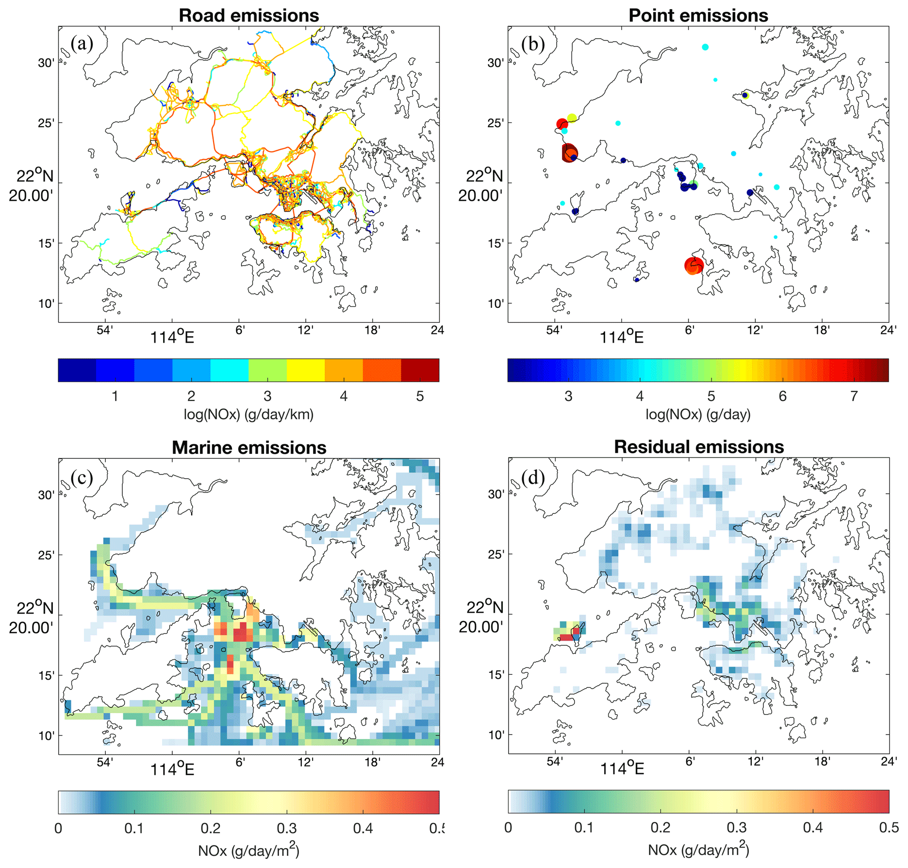
Figure 2Emission maps of NOx provided by Hong Kong EPD for the Hong Kong region from road (a), point (b), marine (c), and residual (d) sources. The road emissions are shown as line sources for every road (in g d−1 km−1). For simplification, all the roads, including those above and below ground, are added in one layer at the surface. The point sources include power plants, industries, crematoriums, and tank farms (in g d−1 per point). The sizes of the points indicate the height of the source. The marine and residual emissions are area sources provided with a 1 km × 1 km resolution (in g d−1 m−2).
3.1 Surface monitoring network
Hourly averaged air quality monitoring data are obtained from the Hong Kong EPD's network (https://cd.epic.epd.gov.hk/EPICDI/air/station/?lang=en, last access: 13 May 2022). Among all the stations, there are three roadside stations (Mong Kok, Central, and Causeway Bay) and 13 general stations (relative to roadside stations; see Fig. 3). The general stations can be further categorized as urban, suburban, and rural stations. The information about the stations is listed in Table 1. Because of the limitation of the sizes of the inner domains, the observation stations are not covered by all the domains. The mesoscale domains (D01–D04) and the outer LES domain (D05) cover all the stations. For the smaller LES domains, D06 covers all the stations except of the Tap Mun station, and D07 only covers the roadside stations and three general stations. The instrument heights are below 5 m above ground for the roadside stations, while they are between 10 and 30 m above ground for the general stations. We use the first layer of the model data to compare between the surface measurements and the model simulations. During the simulation period, no NOx measurements are available at the Eastern station, and some data are also missing around noon at the Tsuen Wan and Kwai Chung stations.
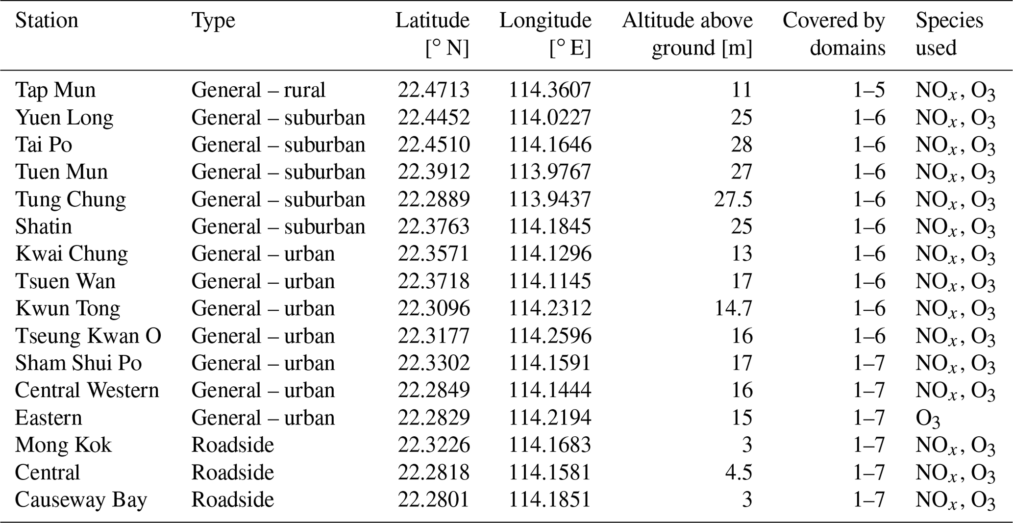
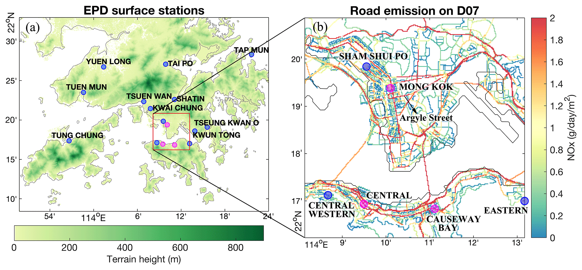
Figure 3Locations of the surface monitoring stations represented on the map of the Hong Kong topography (a) and the road emissions interpolated to D07 domain grids (b). The blue circles represent the general stations, and the magenta circles are the roadside stations.
3.2 Ozone sounding profile
The ozone sounding measurements at the King's Park station (22.311∘ N, 114.172∘ E) in Kowloon Peninsula were conducted by Hong Kong Observatory (HKO). We downloaded the measurement data used for model comparison in this study from the World Ozone and Ultraviolet Radiation Data Centre (WOUDC; https://woudc.org/home.php, last access: 13 May 2022). The profile for the simulation period was derived at 05:55 UTC on 1 August 2018, which corresponds to noontime (13:55 LT) when the convective boundary layer is well developed. The trajectory of the sounding is shown in Fig. 4. For the comparison between models and sounding measurements, the vertical profiles are usually taken at the location of the site because of the coarse resolution of the models. In fact, the sounding balloon drifted over large horizontal distances in response to the background winds during its ascent. In the case adopted in the present study, the balloon drifted about 1.4 km away from its release location before it reached the level of 2 km, and it drifted over a distance of 8.6 km at 10 km altitude. Therefore, as for the high-resolution model simulations in this study, we adopt the nearest model grids along the sounding trajectory for a more precise comparison.
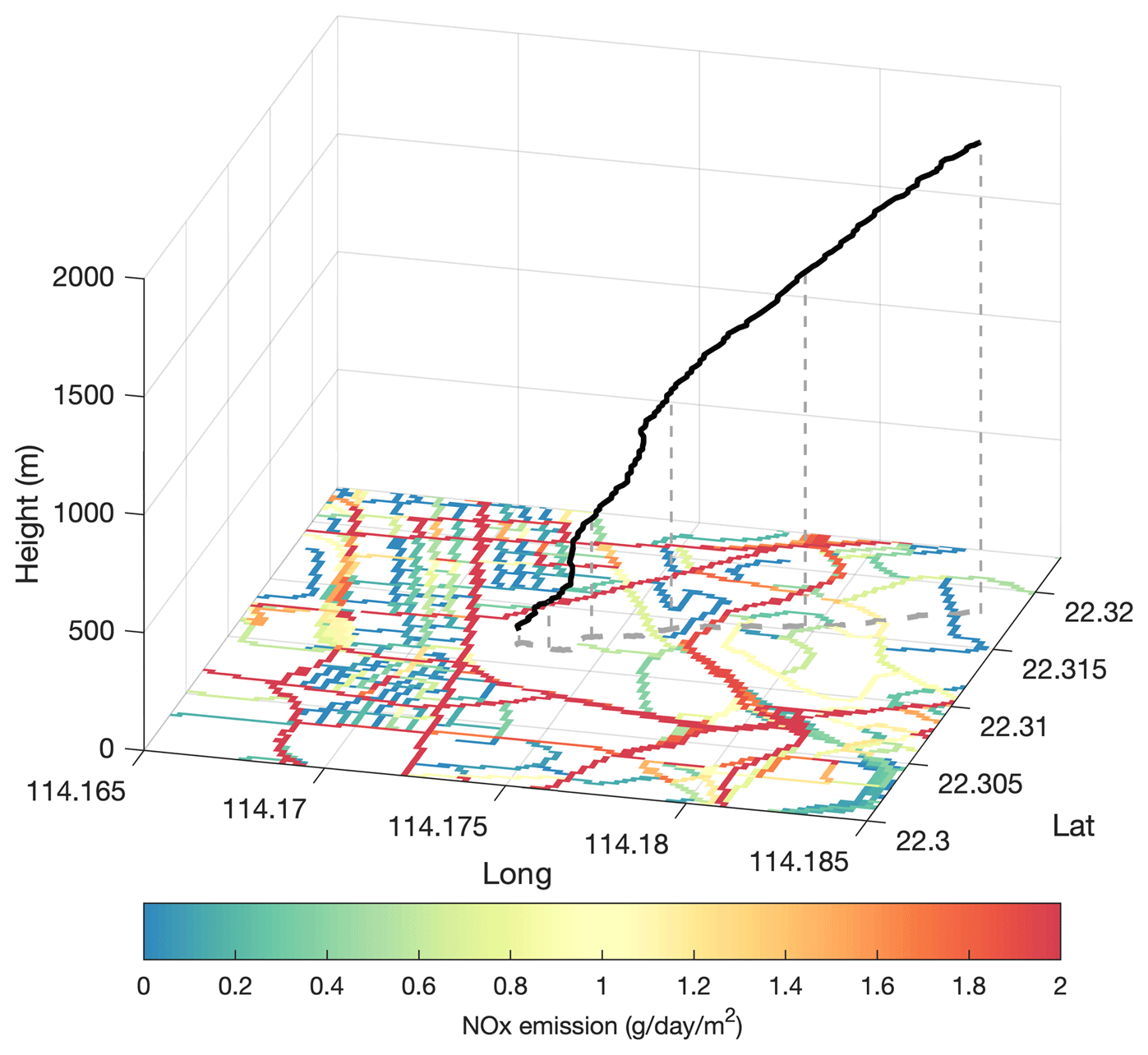
Figure 4Ozone sounding trajectory in the first 2 km over the road emission map adopted for the innermost domain D07.
4.1 General PBL structure
We first evaluate the development of the boundary layer structure in the simulations by comparing model results with sounding profiles at 13:55 LT (Fig. 5). A sharp inversion can be seen in the profiles of the potential temperature and water vapor near the top of the boundary layer, of which this height is usually used to quantify the development of the PBL (Garratt, 1994). For the mesoscale simulations, the PBL height (PBLH) in the model is diagnosed by the YSU PBL scheme. The YSU PBLH for the mesoscale domain (D04, Δ= 900 m) at the nearest grid of the sounding location is 992 m above the surface as shown by the dotted horizontal bar on the D04 profile. In the case of the sounding profiles and the LES model results, the PBLH is determined by applying the bulk Richardson number (Rib) method (Hong et al., 2006), which is similar to the approach used in the YSU scheme. The bulk Richardson number is calculated by
where θv is the virtual potential temperature, θvs is the virtual potential temperature at the surface, u and v are horizontal wind components, and g is gravitational acceleration. The PBLH is defined as the height where Rib first exceeds a threshold value of zero (Hong et al., 2006). The PBLH derived from the relation (1) for D04 is 970 m, which is very similar to the value (992 m) simulated by the YSU scheme. The calculated PBLH are 1132 m and 1204 m for the D06 (Δ= 100 m) and the D07 (Δ= 33.3 m) LES domains, respectively, implying that high-resolution enhances the turbulent mixing and hence raises the boundary layer height. The PBLH derived from the observation profile is 1141 m, which is close to the LES simulations but higher than the value derived in the mesoscale domain D04.
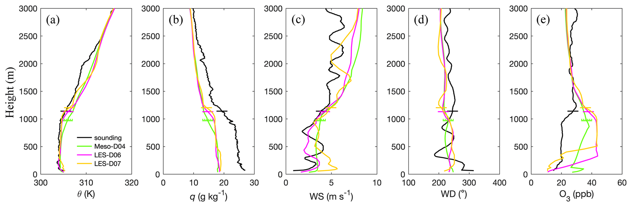
Figure 5Comparison between ozone sounding measurements and model simulations at 13:55 LT. The variables are the potential temperature (θ; a), the water vapor mixing ratio (q; b), wind speed (WS; c), wind direction (WD; d), and ozone mixing ratio (O3; e). The black lines represent observations, the green lines are the simulations from D04 with resolution of 900 m, the magenta lines are the simulations from D06 with resolution of 100 m, and the yellow lines are the simulations from D07 with resolution of 33.3 m. The solid horizontal bars indicate the calculated PBLH for each domain, and the dotted horizontal bars show the simulated PBLH from YSU scheme. To further show the profiles in the boundary layer clearer, the same plot but with the altitudes only up to 800 m is shown in Fig. S4.
The potential temperature is generally satisfactorily represented by the simulations for both the mesoscale and the LES domains. However, the mesoscale simulation overestimates the potential temperature near the PBLH, which explains why the calculated PBLH is lower than the observed value. This suggests that the convection in the mesoscale model is relatively weak at this location. All of the simulations underpredict water vapor consistently among all simulation domains, especially at low altitudes; however, this is consistent among all simulation domains. The basic structure of the wind profiles is reasonably well captured by the simulations, but the large fluctuations caused by local turbulence are difficult to replicate by the model in a deterministic manner. Both mesoscale and LES-scale simulations are able to capture the observed southwesterly wind directions in the lower troposphere, except the near-surface northwesterly winds. This deviation between simulated and observed winds in the near-surface layer is likely due to the local urban morphology effects, which are not included in the WRF model. Additionally, the surface meteorological observations operated by the Hong Kong Observatory (HKO) are used to validate the model simulations. The map of the used stations is shown in Fig. S2, and the comparison of the averaged diurnal variations is shown in Fig. S3. Overall, the coupled mesoscale to LES-scale WRF model is found to be capable of reproducing realistic atmospheric conditions for the period of interest.
4.2 Comparison of ozone profile with sounding measurements
The simulated vertical profiles of ozone are compared to the ozone sounding measurements (Fig. 5). The mesoscale simulation overestimates the ozone concentrations near the surface, probably due to the lack of capability to resolve the road emissions. The emitted NO from traffic sources reacts with O3 to produce NO2:
Under high-pollution conditions, this leads to an increase in NO2 concentrations and a decrease in the O3 level. Therefore, the small emission of NO in the coarse-resolution model results in a weak titration of ozone and hence an overestimation of the ozone concentration. The LES simulations tend to give a lower level of surface O3 due to the better representation of the spatial emission distribution and improve the agreement with the measurements, illustrating the advantage of the high-resolution LES. Both mesoscale and LES simulations overestimate the O3 concentrations within the rest of the PBL above the surface layer, which implies that the O3 source is overestimated in this region. The formation of O3 follows the photolysis of NO2:
The combination of Reactions (R1)–(R3) results in a null cycle without any net gain or loss of O3. However, in the presence of volatile organic compounds (VOCs), the ROx (ROx = OH + HO2 + RO2; RO2 stands for any organic peroxy radical) photochemical cycle continuously supplies HO2 and RO2 to oxidize NO into NO2 without consuming ozone. This mechanism limits the production of O3 in the troposphere (Wang et al., 2017):
where RH represents any non-methane hydrocarbon and RCO represents carbonyls.
To identify the possible reasons for the disagreement between simulations and observations, the vertical cross sections of the O3 mixing ratios along the sounding trajectory for the three domains (D04, D06, and D07) are shown in Fig. 6. This graph shows that the O3 concentrations derived by the mesoscale model are too high within the entire boundary layer depth. In the coupled LES simulations, lower O3 concentrations can be seen near the surface, which agrees with the measurements. The low O3 air masses from the surface can reach approximately 80 % of the PBL height, indicating a strong vertical mixing. In addition, the air parcels with low O3 values are clearly transported to higher altitudes by the updrafts produced by the stronger turbulent mixing occurring in the high-resolution LES domain D07. On the other hand, the downdrafts transport the high O3 air parcels to the lower altitudes (see Fig. 6c). In addition to the low O3 near the surface, high O3 air masses can be found in the west of the domain, resulting in an overestimation of O3 between 400 and 1000 m. The cross sections of OH, HO2, and RO2 are also depicted in Fig. 6 (bottom row), which shows high concentrations of OH, HO2, and RO2 along with the high O3 concentrations. As discussed above, the ROx cycle (Reactions R4–R7) converts NO to NO2 and tends to produce O3 under such conditions. This results in high O3 in the western part of the domain and in the upper boundary layer. The comparison between the models and the observations indicates that the O3 distribution in the LES simulations is offset relative to the measurements – the modeled O3 is shifted to the downwind direction. Figure 5c shows that the model generally overestimates the horizontal wind speed in the boundary layer and therefore displaces the air masses with low O3 too rapidly to the east of the sounding trajectory, which probably explains the overestimation of O3 between 400 and 1000 m.
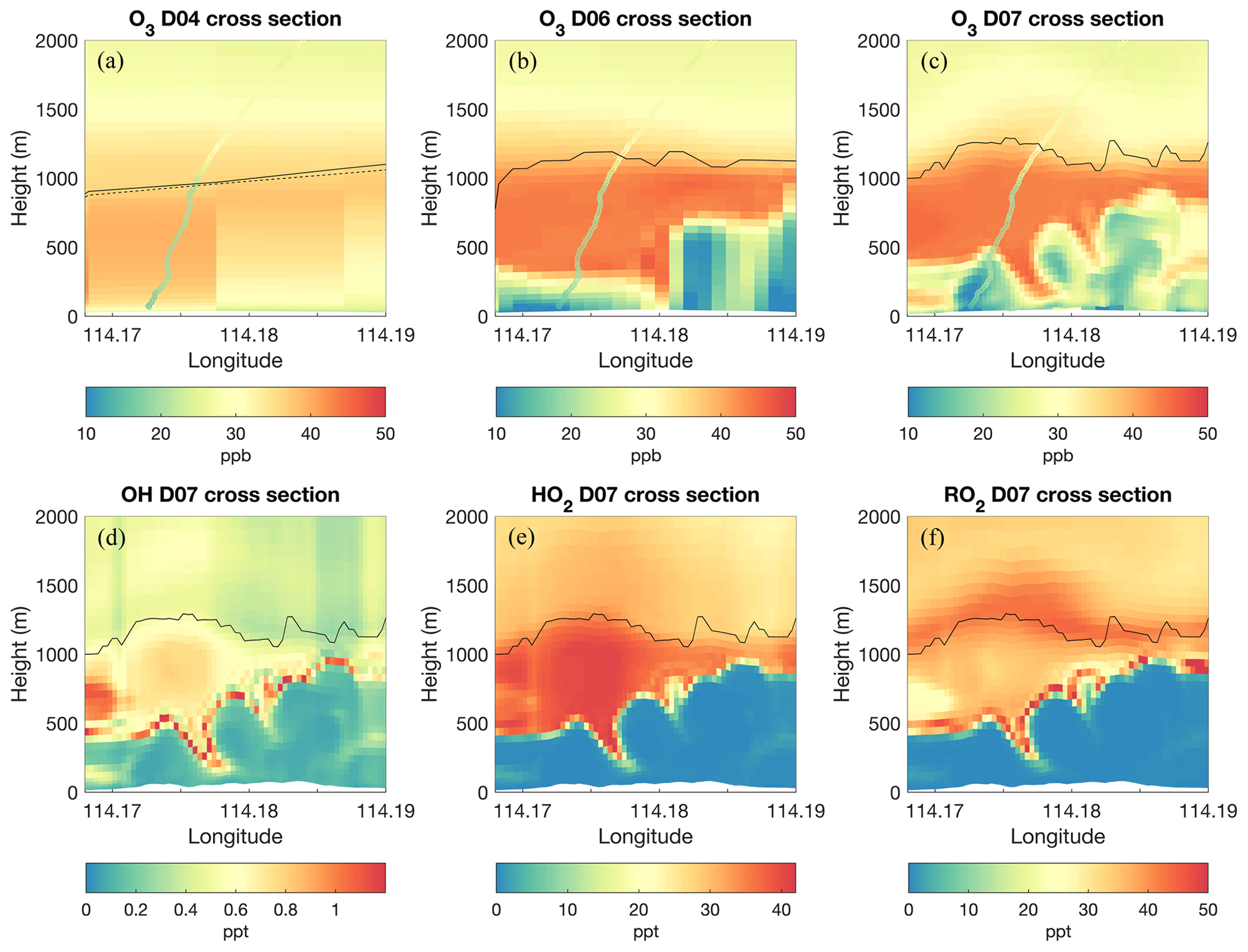
Figure 6(a–c) O3 mixing ratio (ppbv) cross sections along the balloon sounding trajectory for the D04 (a), D06 (b), and D07 (c) domains. Thick colored lines represent the ozone sounding measurements along the trajectories at 13:55 LT. The solid black lines are PBLH calculated using the bulk Richardson number method, and the dashed black line is the PBLH from the model output for the mesoscale domain, which is simulated in the YSU PBL scheme. (d–f) Cross sections along the sounding trajectory for D07 of the OH (d), HO2 (e), and RO2 (f; sum of the organic peroxy radicals in RADM2 chemical mechanism) mixing ratios (pptv).
4.3 Comparison of pollutants with surface observations
Figure 7 shows a comparison between simulated NOx concentrations and surface measurements. We focus here on the model results from the innermost mesoscale domain (D04, 900 m, green dots), the middle LES domain (D06, 100 m, magenta dots), and the innermost LES domain (D07, 33.3 m, yellow dots). At most general stations, the mesoscale simulation of D04 captures the mean NOx concentrations and the diurnal variations well. The best agreement is found at the stations located in the northern and western rural and suburban areas of Hong Kong, i.e., stations that are far away from the city center, including Tap Mun, Yuen Long, Tai Po, Tuen Mun, Tung Chung, and Shatin. The mean NOx concentrations at these suburban stations are lower than 100 µg m−3. This indicates that the regional models are good at predicting the background levels of the pollutants over a relatively large area. For the urban general stations closer to the emission sources, the simulated NOx concentrations in the D04 case are higher than the measured values except at the Kwun Tong station. The overestimation of NOx mainly occurs during the rush hours (07:00–09:00 and 18:00–20:00 LT), implying that the road emissions are overestimated at these locations. As for the roadside stations, as expected, the NOx values are underestimated in the mesoscale simulation due to the poor representation (too coarse resolution) of the road emissions. The mean biases (MBs) and root-mean-square errors (RMSEs) of the simulated versus measured NOx concentrations are listed in Table 2. The smallest MBs are found at the suburban stations, most of which are below 15 µg m−3. The RMSEs at these stations are between 15 and 45 µg m−3. At the urban general stations, the only negative MB is found at the Kwun Tong station, where the mesoscale D04 simulation underestimates the observed NOx. The MBs at the other urban general stations are all positive, ranging between 30 and 50 µg m−3. The RMSEs at the urban general stations are 30–60 µg m−3. The MBs and RMSEs for the roadside stations are much higher than those of the general stations. The MBs are all negative at the roadside stations with values of −97.006 µg m−3 at Mong Kok, −54.373 µg m−3 at Central, and −171.499 µg m−3 at the Causeway Bay station. The RMSEs range from 117.431 to 219.693 µg m−3 for the roadside stations.
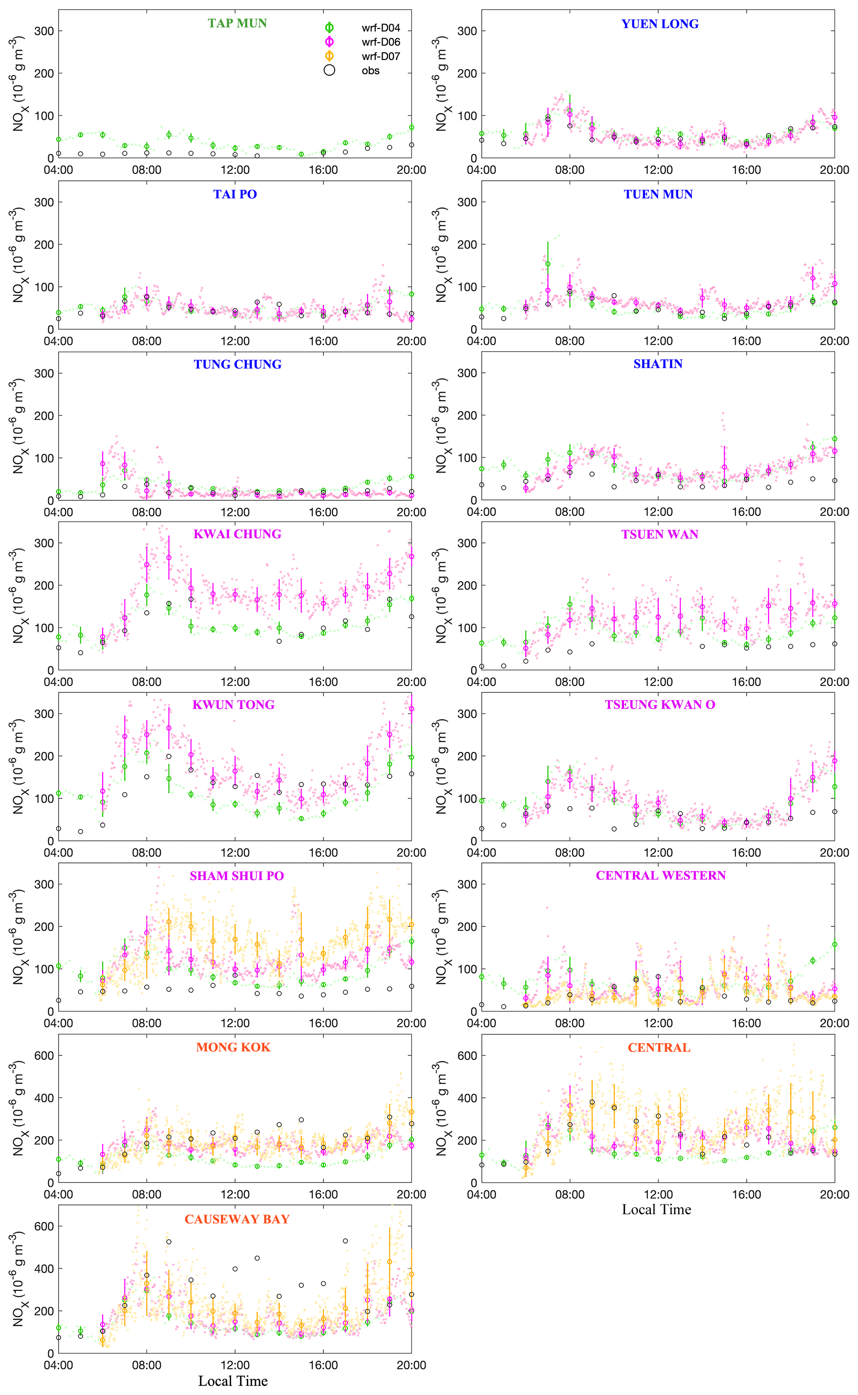
Figure 7Comparison between NOx surface measurements and model simulations. Black circles are hourly observations; small dots with different colors (green: D04; magenta: D06; magenta: D07) represent the simulations at output intervals. Dots with error bars refer to the hourly averages with standard deviations. Note that the y axis is different for the general and roadside stations. The station names are marked with different colors to represent the station types: green is rural, blue is suburban, magenta is urban, and red is roadside.
Table 2Statistical parameters to evaluate the modeled NOx against surface measurements in Hong Kong EPD's network. Both mean bias (MB) and root-mean-square-error (RMSE) values are given in units of µg m−3.
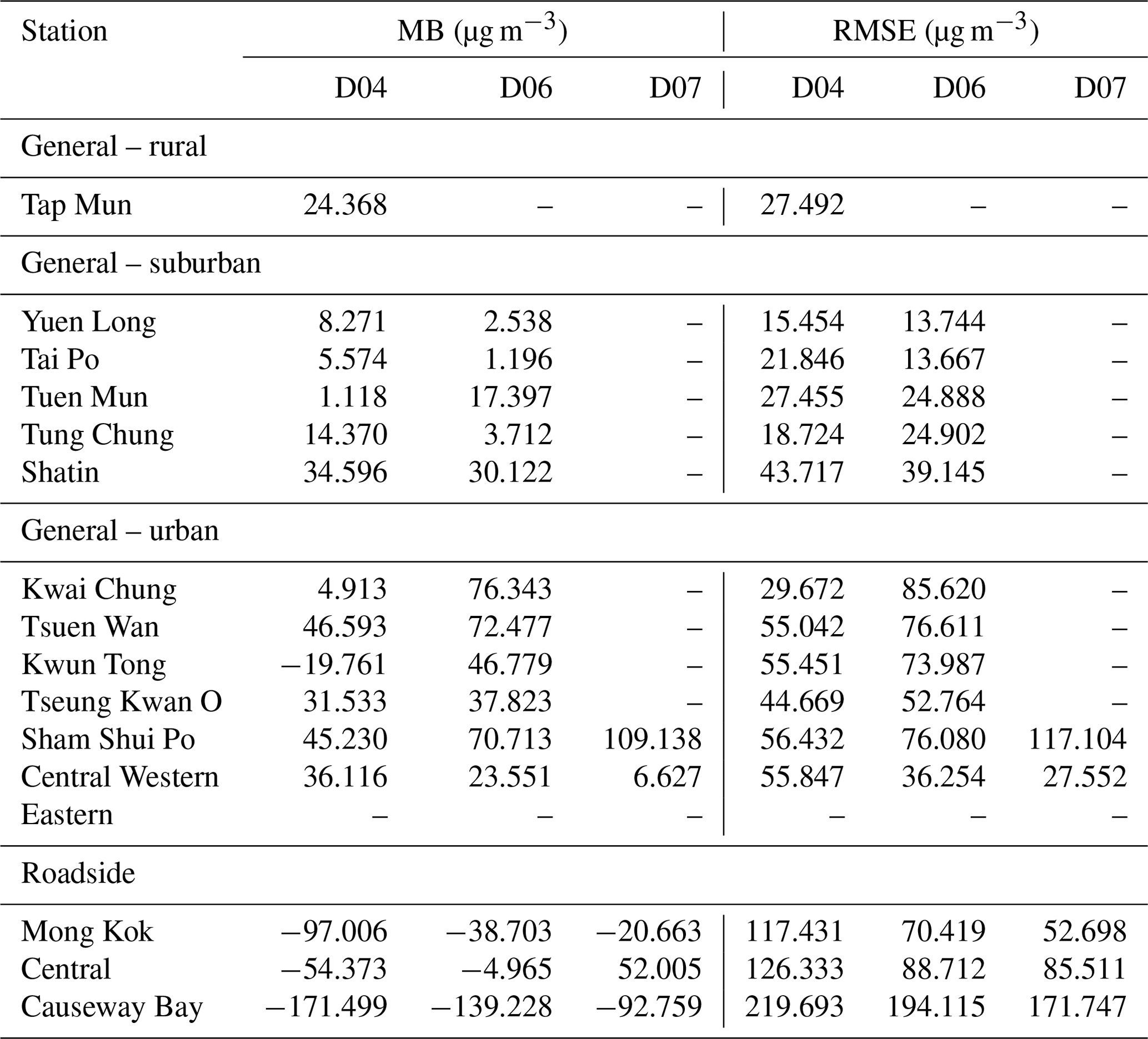
The 100 m LES (D06) simulation results in mean concentrations and diurnal variations of NOx that are similar to those from the mesoscale model at the suburban stations, but with larger variances resulting from the explicitly resolved eddies. Some improvements can be seen during evening hours at Tai Po and Tung Chung. The calculated MBs and RMSEs show improvement in the D06 LES simulation at most of the suburban stations when compared to the mesoscale simulation. For example, at the Tai Po station, the MB decreases from 5.574 µg m−3 in the D04 simulation to 1.196 µg m−3 in the D06 simulation, and the RMSE decreases from 21.846 to 13.667 µg m−3. The variances of the simulated NOx concentrations from D06 are larger at the urban stations closer to the city center, indicating the complexity of the mixing and dispersion of pollutants in the turbulent flows over heterogenous urban surfaces even without the explicit representation of buildings. The agreement between the NOx concentrations simulated by the 100 m LES and by the measurements is improved at the Central Western urban stations with smaller MB and RMSE and is worsened at the other urban general stations (e.g., the 100 m LES overestimates the NOx concentrations at Tsuen Wan, Kwai Chung, Kwun Tong, and Sham Shui Po). In other words, the high-resolution model does not necessarily provide better predictions of the chemical species at the general stations. One possible explanation is that the emission inventories (or their spatial and temporal resolution) are not sufficiently accurate and resolved in time. For instance, the road emissions are based on annual mean traffic flows and their mean diurnal profile, which do not capture the real-time variations. In addition, the road emissions on the overpass are added to the surface layer and thus result in higher NOx in the simulations at the surface. Also, while higher resolution than standard mesoscale predictions, the LES domains used here do not allow explicit resolution of buildings, which is expected to have a considerable impact in capturing local effects within the urban canopy. As for the roadside stations, the improvements of the 100 m LES simulation are clearer. The D06 simulation provides larger NOx values than the D04 simulation and agrees more closely with the measurements. This can be seen from the decreased negative biases: MB decreases by about 60, 50, and 30 µg m−3, at Mong Kok, Central, and Causeway Bay, respectively. The RMSEs are also reduced at the three roadside stations. However, there are still disagreements between the D06 simulations and the measurements; for example, the case at Causeway Bay and between 09:00–12:00 LT at the Central station.
When the LES grid size is decreased to 33.3 m (D07), the agreement between the simulation and the observations is further improved at the roadside stations. Large improvements can be seen at the Central station in the morning; however, the agreement is worse in the evening. This results in a larger mean bias at the Central station compared to the D06 simulation. The MB at Mong Kok decreases from −38.703 µg m−3 in the D06 simulation to −20.663 µg m−3 in the D07 simulation and reduces from −139.228 to −92.759 µg m−3 at the Causeway Bay station. For the two urban general stations covered by the D07 domain (note that the Eastern station is covered by D07 but has no NOx data for the simulation day), the D07 simulation improves the agreement with the measurements at Central Western, with the corresponding MB reducing from 23.551 to 6.627 µg m−3 and the RMSE decreasing from 36.254 to 27.552 µg m−3. However, Both MB and RMSE increase at the Sham Shui Po station. The comparison between simulations and observations indicates that increasing the model resolution does not necessarily lead to an improvement over the background air quality simulation, although it can provide a better representation of the air pollution structure over complex land surfaces and near the emission sources.
Next, we compare the simulated ozone concentrations against the observations (refer to Fig. 8), and the statistical skill metrics are listed in Table 3. The interpretation of ozone simulations is more complex because, as opposed to the case of a primary pollutant with a short lifetime like NOx that is largely controlled by surface emissions, O3 is also affected by chemical transformations, dynamic transport, and turbulent mixing. As seen from most of the stations in Fig. 8, the diurnal evolution of the surface O3 is characterized by low values in the morning and evening and by high values during daytime with a concentration peak occurring around 14:00 LT, which is when the photochemical production is largest. The lower O3 concentrations at the roadside stations compared to those at the general stations are characteristic of an environment that is NOx saturated and hence VOC limited. Overall, the mesoscale simulation from D04 matches the observations well at the general stations, suggesting that the representation of the physical and chemical processes in the model is sufficiently realistic. The D04 simulation slightly overestimates the O3 concentrations at most general stations during daytime but underestimates O3 in the morning and evening, which is partly attributed to the NOx overestimation during the rush hour, resulting in the overestimated titration of ozone by NO. The positive MBs at the general stations mostly range from 0.6 to 6.6 µg m−3, except at the Tung Chung station near the airport in the west of Hong Kong, where it reaches 12.970 µg m−3. The negative MBs are in the range between −0.331 and −4.463 µg m−3 and mostly occur at the stations in the east of Hong Kong, implying that the model underestimates the O3 concentration in that region, possibly due to the strong transport of NOx towards the east by the westerly winds as discussed in Sect. 4.2. The RMSEs at the general stations are estimated to be between 8.416 and 25.257 µg m−3, and the largest value is found at the Eastern station. The O3 concentrations are overestimated by the mesoscale simulation at the roadside stations as a consequence of the low NOx traffic emissions in the coarse model. The MBs are 11.671 µg m−3 at Mong Kok, 6.208 µg m−3 at Central, and 9.830 µg m−3 at Causeway Bay, and the corresponding RMSEs are 18.079, 13.792, and 18.551 µg m−3, respectively.
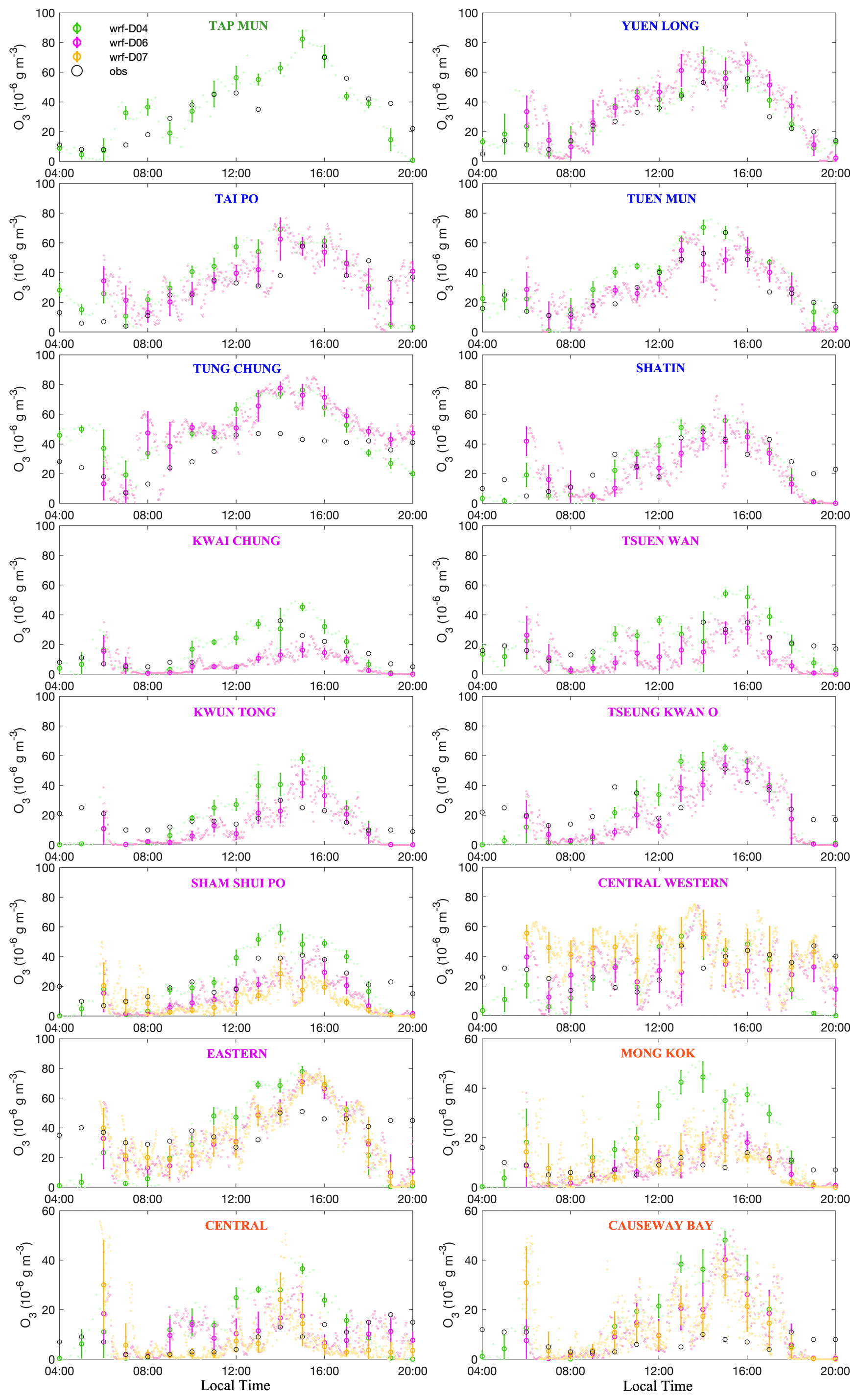
Figure 8Comparison between O3 surface measurements and model simulations. Black circles are hourly observations; small dots with different colors (green: D04; magenta: D06; magenta: D07) represent the simulations at output intervals. Dots with error bars refer to the hourly averages with standard deviations. Note that the y axis is different for the general and roadside stations. The station names are marked with different colors to represent the station types: green is rural, blue is suburban, magenta is urban, and red is roadside.
Table 3Statistical parameters to evaluate the modeled O3 against surface measurements in Hong Kong EPD's network. Both mean bias (MB) and root-mean-square error (RMSE) values are given in units of µg m−3.
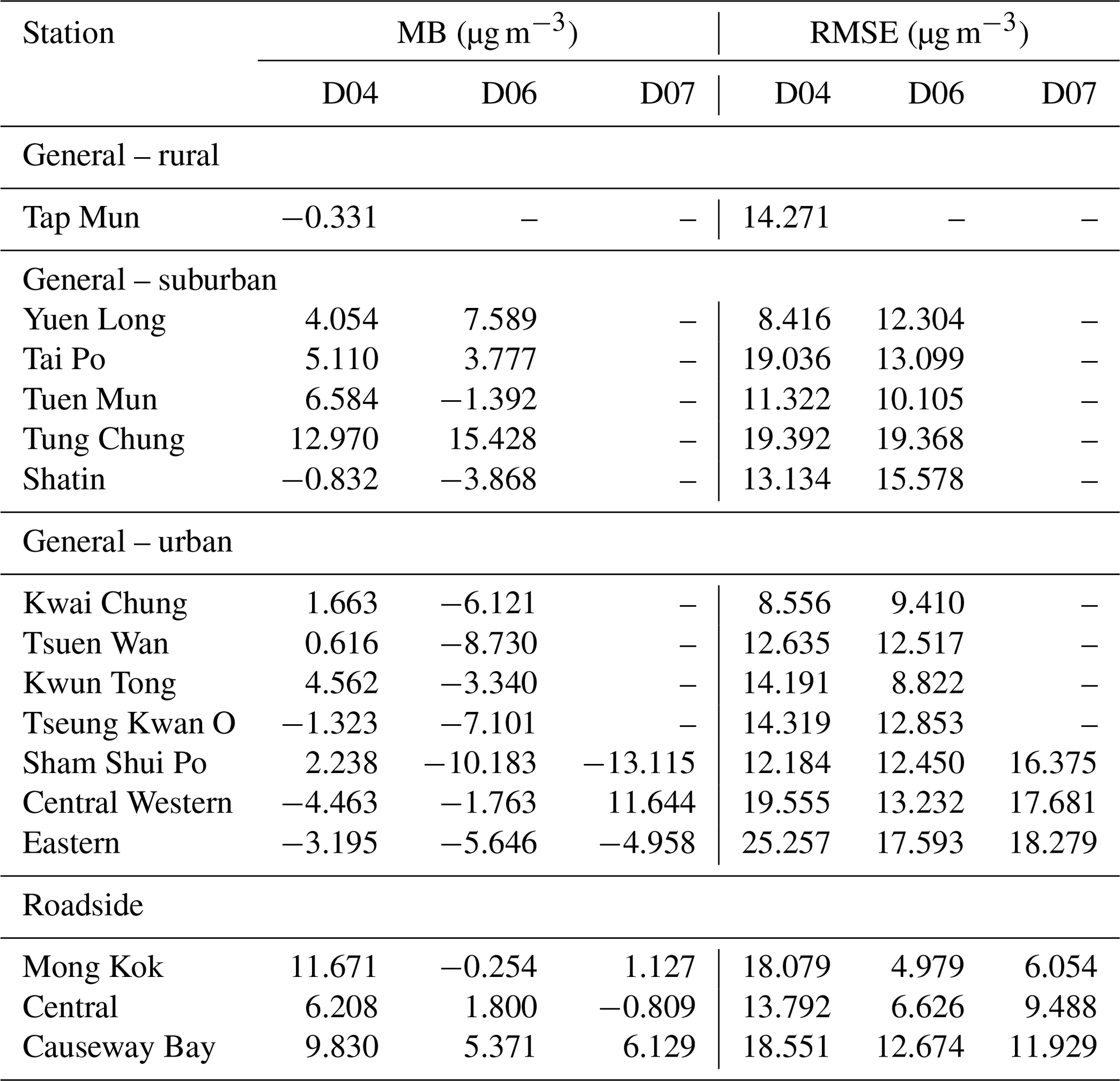
When the LES simulation is performed at a 100 m resolution (D06), the O3 concentrations are reduced at most of the general stations except at the Yuen Long, Tung Chung, and Central Western stations. Since the mesoscale simulation overestimates the observed O3 concentrations, this reduction in the O3 concentration slightly improves the agreement with measurements. The LES also reduces the ozone discrepancies in the evening at the Tai Po, Tung Chung, and Central Western stations. However, the calculated MBs and RMSEs do not show consistent improvement. As for the roadside stations, where a lower level of O3 concentration is often observed, the simulated O3 concentrations reproduce the observation better, especially at Mong Kok. With the D06 simulation, the agreement at the Central station is also improved; however, there are some discrepancies during the morning rush hour. The improvement at Causeway Bay is relatively limited. Both MBs and RMSEs decreased compared to the D04 simulation. The MB is reduced from 11.671 to −0.254 µg m−3 at Mong Kok and from 6.208 to 1.800 µg m−3 at the Central station; the change ranges from 9.830 to 5.371 µg m−3 at Causeway Bay. The reductions of RMSEs are approximately 13, 7, and 6 µg m−3, for Mong Kok, Central, and Causeway Bay, respectively.
In the case of ozone, the high-resolution LES simulation (D07) does not provide improved results at the three general stations and even slightly degrades the model performance relative to the D06 simulation. The MBs from the D07 simulation at Sham Shui Po and Central Western are larger than those from D06, and the MB at the Eastern station decreases slightly from −5.646 µg m−3 for D06 to −4.958 µg m−3 for D07. The RMSEs increase modestly at all three general stations. However, as shown in Fig. 8, some improvements can be noticed at the roadside stations. For instance, in the D07 simulation the O3 concentrations are reduced during the morning hours at the Central station, showing a better match with the observation. Although the hourly mean values of O3 from D07 are still too high in the afternoon at Causeway Bay, the observed values are in the range of the variability produced by the high-frequency model output. The MB decreases from 1.800 to −0.809 µg m−3 at the Central station, while the MBs slightly increase at Mong Kok and Causeway Bay. The presented comparison with surface measurements highlights the existence of larger fluctuations in the pollutant concentrations, which the high-resolution LES model is able to capture in response to more complex turbulent flows in the urban area. These fluctuations may bring the concentrations of the chemical species closer to the range of measurements without substantially modifying the average values derived from the statistical analysis of the LES output.
4.4 Spatial distribution of the pollutants
Having validated the model with observations, we now analyze the representation of the spatial distribution of pollutants at different model resolutions. The horizontal distributions of NO, NO2, and O3 near the surface for three different model resolutions are shown in Figs. 9 and 10 at 06:00 LT (morning) and 13:00 LT (noon), respectively. These two times are selected to represent different boundary layer conditions and traffic emissions. To better characterize the differences between model resolutions, we examine our results only in the subregion of D07, which is located in the city center of Hong Kong and is subject to strong traffic pollution. This region corresponds to the area covered by D07, but with the southern and western edges of the domain removed to limit the influence from the mountains and the ocean.
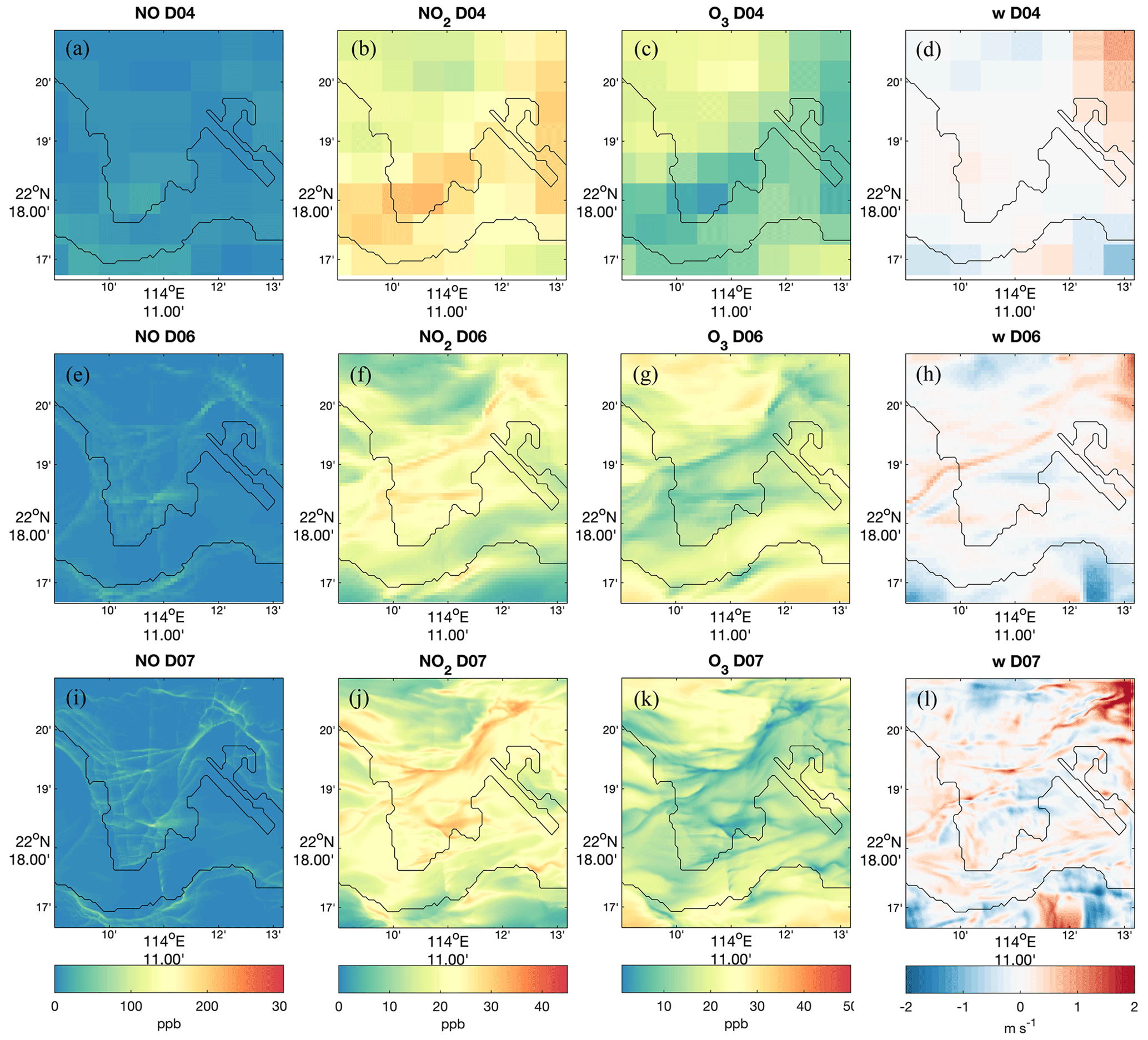
Figure 9Horizontal distribution of simulated NO (first column), NO2 (second column), and O3 (third column) near the surface at 06:00 LT for the D04 (first row), the D06 (second row), and the D07 (third row) cases. The fourth column provides the horizontal distribution of vertical wind (w) at approximately 100 m above ground.
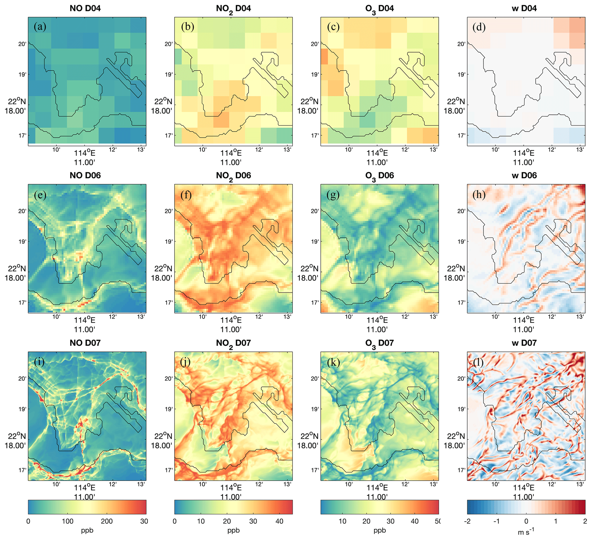
Figure 10Horizontal distribution of simulated NO (first column), NO2 (second column), and O3 (third column) near the surface at 13:00 LT for the D04 (first row), the D06 (second row), and the D07 (third row) cases. The fourth column provides the horizontal distribution of vertical wind (w) at approximately 100 m above ground.
At 06:00 LT, around sunrise, the NO concentrations are very low because NO has been consumed by the O3 during the night, and the photolysis of NO2 is still weak at 06:00 LT. Additionally, the rush hour usually starts at 08:00 LT, meaning that the direct emission of NO from the road traffic is weak. In the case of the mesoscale domain, the horizontal distribution of chemical species in D04 appears in Fig. 9 as mosaic tiles with little spatial variation due to its coarse model resolution (see the first row in Fig. 9). In the case of the LES domains D06 and D07, the road NO emissions can be seen on the maps; in particular, the 33.3 m LES produces a distribution of NO in which the presence of the streets is clearly visible. Due to the morning transition, the dispersion of the NO is very weak in the early morning. Contrary to the situation with NO, NO2 is not directly emitted at the surface, but it is rapidly produced by the conversion from NO. Therefore, the distribution of NO2 is not as concentrated along the traffic routes as that of NO but is more influenced by the air flows. In the early morning, the boundary layer transits from stable to unstable conditions, and the combined effect of shear and surface heating plays an increasingly important role in turbulence generation (Beare, 2008), causing the flow to evolve into horizontal rolls oriented along the mean wind direction (southwesterly in this case, see Fig. 9h, l). As a result, a clear strip-like structure associated with convective rolls is visible in the NO2 distribution patterns, especially in the LES model with 33.3 m resolution (see Fig. 9j). Similarly, the O3 distribution is influenced by the air flow, showing an opposite feature compared to the pattern of NO2 since surface O3 is strongly titrated by NO. To some extent the spatial distribution of NO2 and O3 can be explained by the pattern of vertical wind speed (Fig. 9h, l). The narrow strip-like updrafts in the southwesterly direction transport the high surface NO upwards to consume O3, resulting in narrow regions of high (low) concentrations of NO2 (O3) above the near-surface layer.
At 13:00 LT, the NO concentrations are higher than those at 06:00 LT due to increased traffic emissions during daytime (see Fig. 10). Moreover, the NO emitted on the streets exhibits an obvious diffusion phenomenon in the LES domains at noontime in response to the enhanced turbulent mixing and the higher-resolution emission distribution applied to the model. The changes with time in NO2 and O3 concentrations at different locations and with different model resolutions are partially due to the complex photochemical reactions. After sunrise, convective instability in the PBL gradually increases, which causes the stronger turbulent mixing, and the structure of turbulent flows changes from roll-like to cell-like patterns, yet is disturbed by the presence of terrain and land cover heterogeneities. This can be seen from the cellular structures of the vertical wind speeds and specifically from the comparable intensity of stronger narrow updrafts and wide downdrafts in the more convective boundary layer (see Fig. 10l). Such stronger mixing results in clearly cellular structures in the NO2 and O3 concentration distribution at noontime in the LES D07 domain but not in the mesoscale domain D04 and in the coarse-resolution LES D06 domain.
The vertical distributions of the chemical species along the busy east–west Argyle Street (see Fig. 3b) in the vicinity of the Mong Kok station are shown in Fig. 11 (06:00 LT) and Fig. 12 (13:00 LT). In the early morning, the NO concentration is low, and the values are close to zero above the surface, implying weak surface emissions together with weak vertical mixing. The surface NO2 concentration becomes higher than that of NO because of the higher O3 concentrations originating in the upper layers. The low O3 values at the surface are caused by the depletion of this molecule by NO. The vertical rate of mixing in the mesoscale model is parameterized in the PBL, while it is directly calculated in the LES simulations. During the morning period, although the selected PBL scheme and the LES formulation produce similar PBL heights, the LES model produces a more detailed structure that better describes the vertical transport of the pollutants. At noon, the PBL height increases to about 1000 m due to the strong convective instability, which also can be seen from the sounding measurements in Fig. 5. The surface NO concentrations are high along the road associated with the traffic emissions and corresponding high NO2 and low O3 concentration values. The vertical mixing of the chemical species at 13:00 LT is significantly stronger than in the morning because the PBL has become more convective. The vertical transport of the pollutants is higher in the mesoscale simulation than the LESs, especially in the case of NO2. This suggests that the YSU scheme produces strong vertical diffusion. Compared with the coarse-resolution LES case (D06), the width of the high NO2 and low O3 concentration patterns within the PBL in the high-resolution (D07) LES simulation is significantly reduced (about one to several hundred meters), and the width of the low NO2 and high O3 patterns also decreases to the range of several hundred meters to 1 km. This is related to the thermal structure characterized by narrow updrafts and wide downdrafts during the well-developed phase of the turbulent PBL (see Fig. 12l), which is subject to under-resolved convection effects widening these thermals at coarser grid spacings.
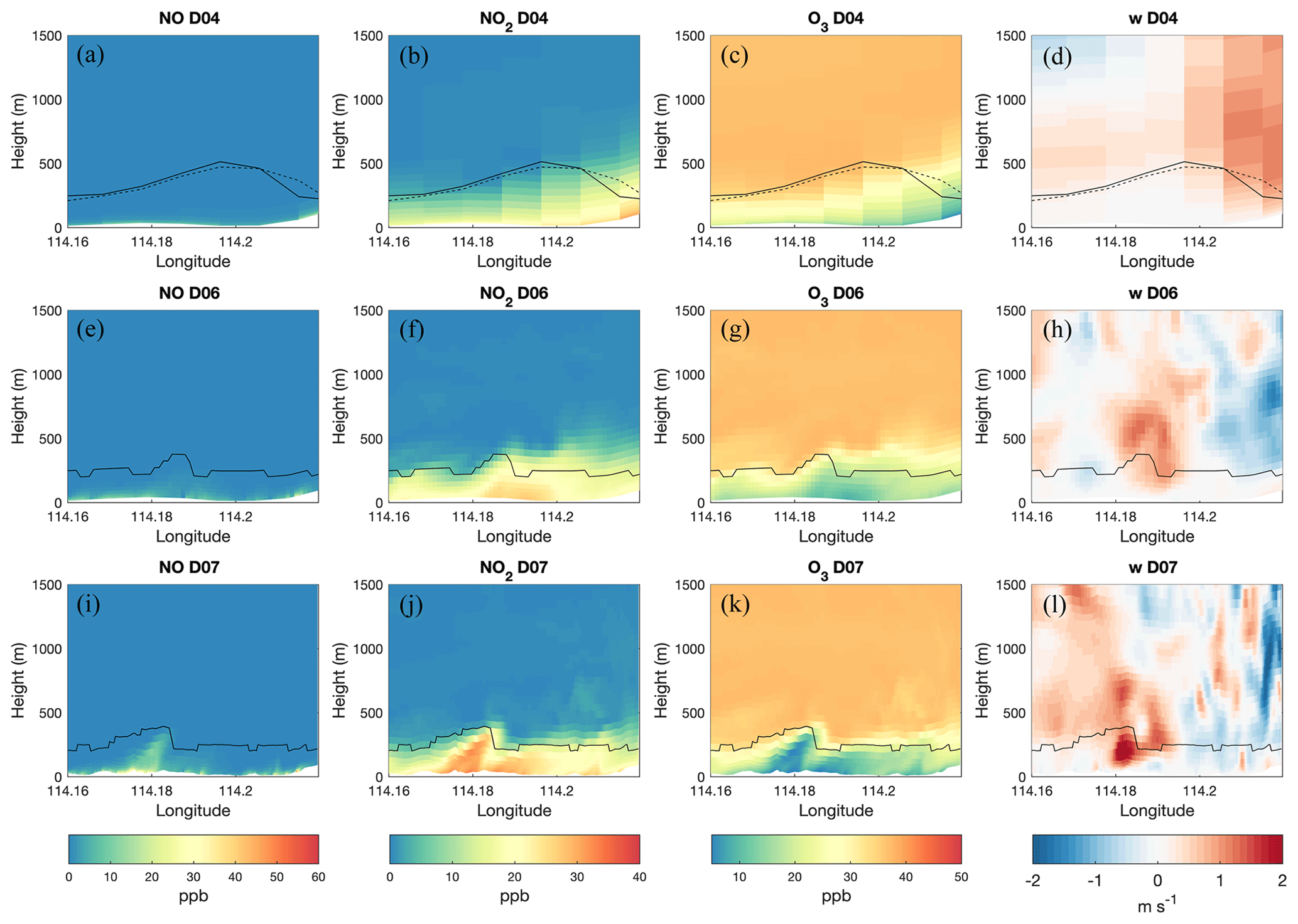
Figure 11Vertical distribution of simulated NO (first column), NO2 (second column), O3 (third column) mixing ratios (ppbv) and vertical wind velocity (w; fourth column) along a busy east–west road near the Mong Kok station (Argyle Street; see Fig. 3b) at 06:00 LT for the D04 (first row), D06 (second row), and D07 (third row) cases. The solid black lines represent the calculated PBLH, and the dashed black line represents the PBLH from the model output for the mesoscale domain, which is calculated in the YSU PBL scheme.
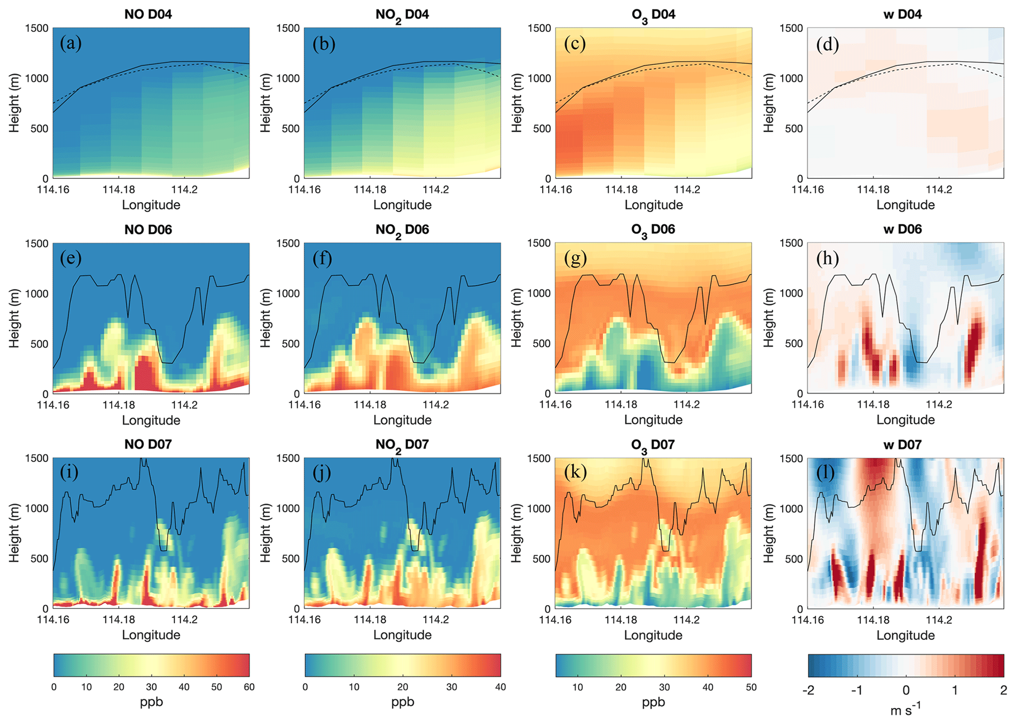
Figure 12Vertical distribution of simulated NO (first column), NO2 (second column), O3 (third column) mixing ratios (ppbv) and vertical wind velocity (w; fourth column) along a busy east–west road near the Mong Kok station (Argyle Street, see Fig. 3b) at 13:00 LT for the D04 (first row), D06 (second row), and D07 (third row) cases. The solid black lines represent the calculated PBLH, and the dashed black line represents the PBLH from the model output for the mesoscale domain, which is calculated in the YSU PBL scheme.
4.5 Development of vertical mixing of pollutants over a diurnal cycle
As shown in Sect. 4.4, the vertical structure of the pollutants significantly varies with different model resolutions. To further evaluate the model behavior regarding the overall vertical mixing, the spatial and temporal averaged (over the subregion plotted in Figs. 9–10 and within 1 h) profiles of the chemical species at different times of the day are shown in Fig. 13. To aid the interpretation of the vertical mixing with the boundary layer development, the diurnal variation of PBLH for selected domains is shown in Fig. 14. The PBLH is only about 200–300 m in the early morning when the boundary layer is still stable. As solar radiation intensifies, the PBLH starts to rise and reaches about 400–500 m at 08:00 LT. The PBLH continues to increase during the morning and reaches the highest altitude at noon. The mean PBLH derived for the selected area D04 is 1088 m at 13:00 LT, which is similar to the height calculated for the sounding profile at the King's Park station. However, the mean PBLH is 768 m in the D06 LES simulation, which is considerably lower. This is possibly due to the local dynamics as seen in Fig. 12. The D07 LES is producing a PBLH (977 m) that is higher than the D06 LES simulation but still 100 m lower than the mesoscale simulation. This indicates that the D06 LES underestimates the strength of the convective motions as it does not resolve turbulent eddies as accurately as the high-resolution LES (D07). In the afternoon, as the surface heat becomes weaker, the PBLH gradually decreases. After sunset, the boundary layer becomes stable again, and the PBLHs decline rapidly to 393, 284, and 280 m, respectively, for the three domains.
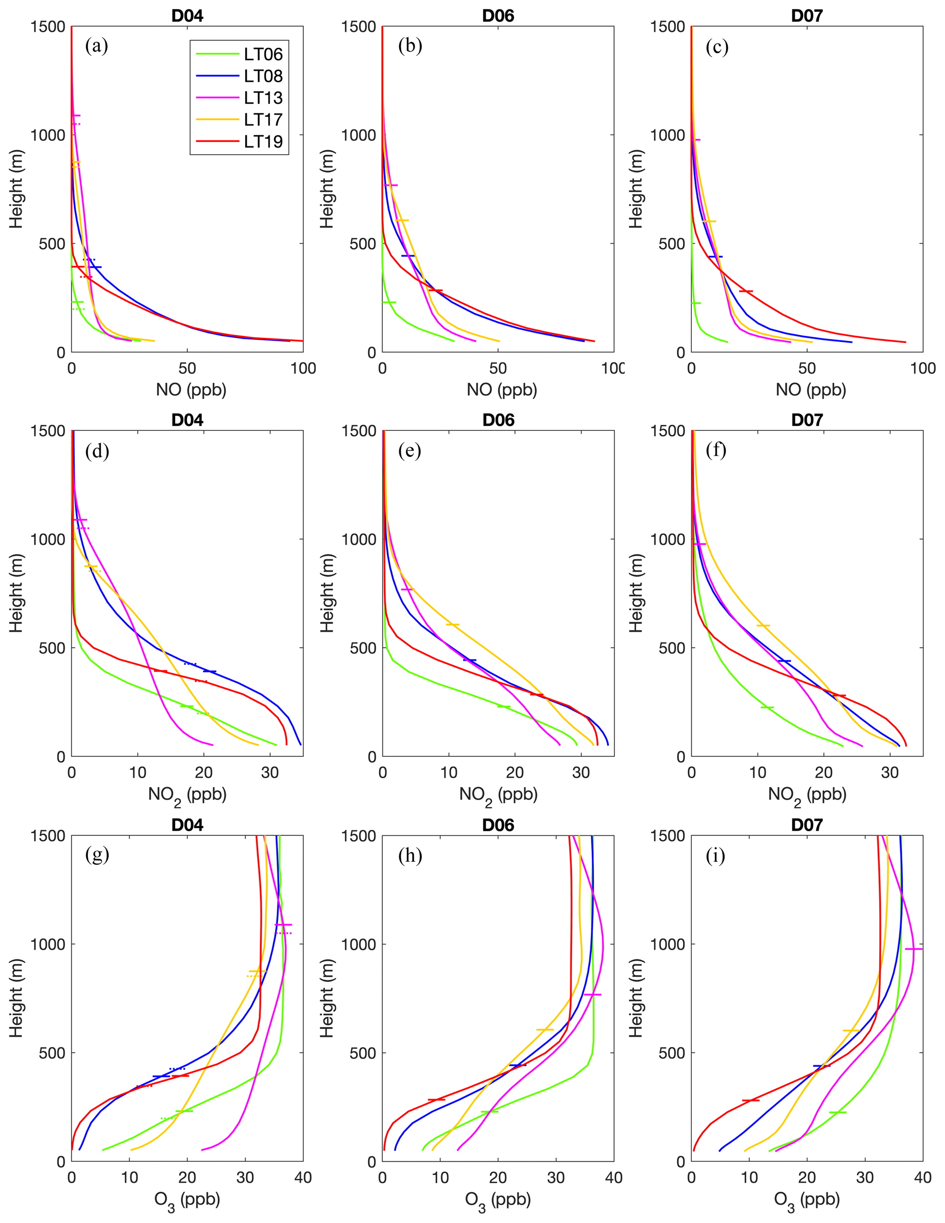
Figure 13Horizontally averaged hourly mean profiles for the mixing ratio (ppbv) of chemical species (NO, NO2 and O3) over the plotted region in Figs. 9–10 for the diurnal cycle on 1 August 2018. Different colors represent different times of the day: green is 06:00 LT, blue is 08:00 LT, magenta is 13:00 LT, yellow is 17:00 LT, and red is 19:00 LT. (a, d, g) Simulation for D04 with a resolution of 900 m. (b, e, h) Simulation for D06 with a resolution of 100 m. (c, f, i) Simulation for D07 with a resolution of 33.3 m.
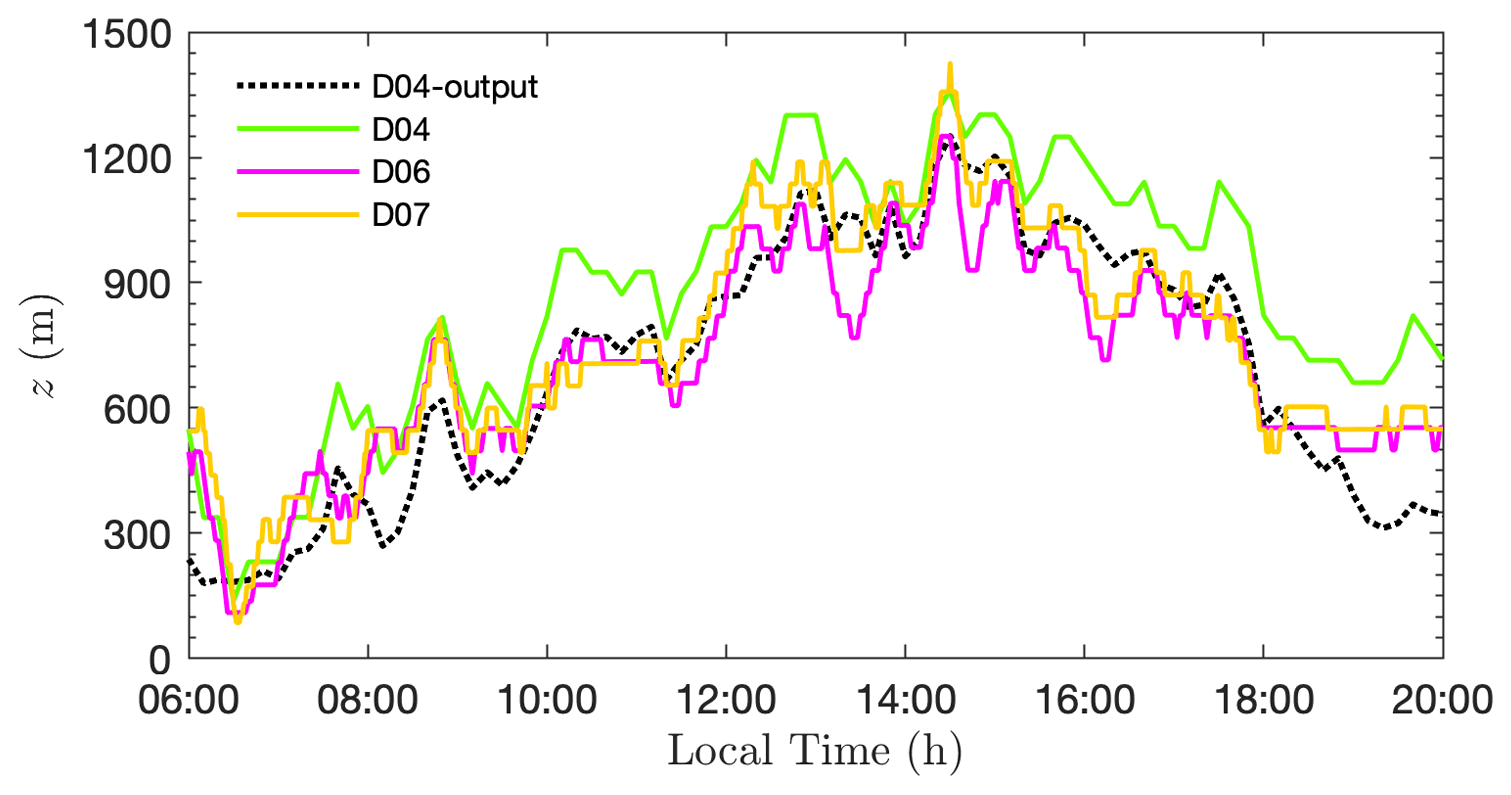
Figure 14Horizontally averaged PBLH over the plotted region in Figs. 9–10 over the diurnal cycle on 1 August 2018. The different colors of the solid lines represent different model resolutions: green is D04 (900 m), magenta is D06 (100 m), and yellow is D07 (33.3 m).
The simulated NO concentrations are highest near the surface and decrease rapidly against altitude. The mean NO concentrations are between 20 and 30 ppb at the lowest layer of the model in the early morning and decline by a factor of 10 to 1–3 ppb at the PBLH. At about 200 m, the high-resolution LES (D07) provides lower NO concentrations relative to the low-resolution LES (D06) and the mesoscale simulation (D04). In other words, the vertical transport of NO is weakest in D07 in the early morning. As the strength of traffic pollution increases during the morning rush hour, the surface NO concentrations increase rapidly to 70–90 ppb in the three simulations and reach values that are about 3 times higher than those at 06:00 LT. The coarse-resolution model produces surface NO values that are larger than in the high-resolution LESs; however, the NO concentrations at the PBLH are about 10 ppb in all three simulations, with higher PBLH derived in the LES simulations. This implies the faster development of the boundary layer and the stronger vertical mixing in the high-resolution LES. The surface concentration of NO decreases around noon due to the reduction in the road emissions after rush hour. In contrast with the morning profiles, the D07 LES simulation exhibits high surface NO concentrations. Indeed, values derived in the D07 case are about twice as high as the values produced by the mesoscale simulations. However, the vertical mixing of NO above 500 m is stronger in the mesoscale simulation in which the PBL is parameterized. This is related to the higher PBLH produced in the D04 simulation for the convective dominated noon condition. The strong vertical transport extends into the afternoon, and the profiles at 17:00 LT are similar to those at 13:00 LT. The NO concentrations above 500 m start to decrease in the evening as the PBL height decreases; however, the surface NO concentration rises again during the evening rush hour at 19:00. In the high-resolution LES simulations it also shows significantly higher NO concentrations in the residual layer.
The patterns that characterize the NO2 mean profiles are different from those of NO. The peak values of NO2 are also located at the surface, due to the large amount of NO, but the decay rate against altitude is slower than that of NO. At 06:00 LT, the surface NO2 concentrations are about 30 ppb in the D04 and D06 simulations and approximately 25 ppb in the D07 LES case. The corresponding concentrations at PBLH are 17, 18, and 12 ppb for the three simulations, equivalent to approximately 50 % of the surface level concentrations. Compared to the other two simulations, the D07 LES exhibits higher NO2 concentrations above the PBLH, implying strong conversion of NO to NO2. With the increase in traffic emissions in the morning rush hour at 08:00 LT, the NO2 concentrations did not rise as much as NO, possibly due to the onset of the photolysis. In the morning, the NO2 concentrations in the upper boundary further increase with the development of the convection in the PBL. Similar to the situation with NO, the mesoscale model generates stronger vertical mixing of NO2 at noon compared to the LES simulations. The situation is opposite in the afternoon: the NO2 concentrations near the PBLH at 17:00 LT became lower than the noon time in the mesoscale simulation, while they continue to increase in the D07 LES. This reveals that the decay of convective condition occurs later in the LES than in the mesoscale model. During the evening hours, the air masses with high NO2 values move down with the height of the PBL, and at the same time the surface NO2 concentrations increase due to the continuous surface emissions and the reduction in the photolysis rates.
The O3 concentration profiles generally exhibit opposite patterns relative to NO2 in response to the titration by NO. The O3 concentrations above the boundary layer are mostly influenced by the background levels, which are between 30 and 40 ppb. In the early morning the surface O3 concentration is about 5 ppb in the D04 case, 7 ppb in the D06 case, and 12 ppb in the D07 case, respectively; these values are related to the NO concentrations in the different simulations. The surface O3 is reduced at 08:00 LT by the depletion of NO that is released by traffic emissions during rush hour. The O3 levels in the mixed layer are replenished through subsidence from the upper layers during the day, which results in the rise of O3 during the afternoon. In the evening, O3 concentrations decrease again because of the slower downward transport and the titration by the NO emitted from traffic roads.
The vertical fluxes of the chemical species are calculated for the LES simulations with different horizontal resolutions. The horizontally averaged flux profiles over the selected region at different times are shown in Fig. 15. For NO, the vertical fluxes are positive, indicating net upward transport during the entire diurnal cycle. The peak of the NO fluxes appears to be located between the heights of 100 and 200 m in a layer where the turbulent motion is strong. The vertical fluxes of NO are smallest at 06:00 LT, when the boundary is stable, and then increases substantially with the development of the PBL after sunrise and the increase in traffic emissions around 08:00 LT. This enhancement of the NO fluxes continues into the afternoon as the convection in the PBL keeps growing, and the peaks of the flux profiles are gradually lifted up. The upward transport becomes weaker again in the evening when the boundary layer becomes stable. For NO2, the vertical fluxes are also essentially positive, except right above the PBL in the evening. The peaks in the NO2 upward fluxes are higher than those in NO because of the smaller gradient in the concentration profiles (Fig. 13). The NO2 fluxes above the PBL are larger than the fluxes of NO because of the atmospheric photochemical production of NO2. For O3, the vertical fluxes are generally negative, indicating the downward transport from the upper atmospheric layers, and the pattern of the O3 fluxes is opposite to that of NO2. As expected, the 33.3 m LES produces larger resolved vertical fluxes than the 100 m LES, while the patterns are similar for the two cases. This indicates that the high-resolution LES better represents the turbulent motions and generates stronger vertical mixing in the convective boundary layer. This is consistent with the analysis of concentration profiles.
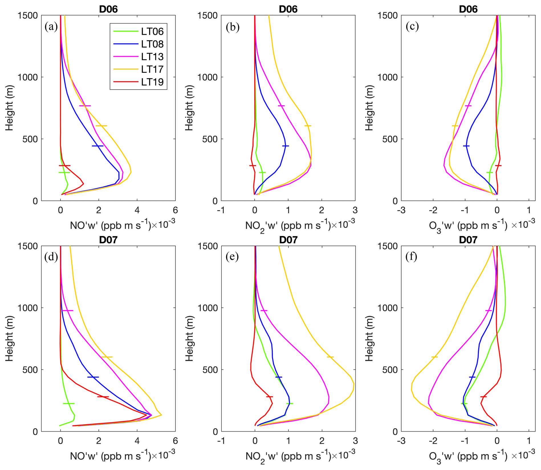
Figure 15Horizontally averaged hourly mean profiles of the vertical fluxes of NO (a, d), NO2 (b, e), and O3 (c, f) in selected regions highlighting the diurnal cycle on 1 August 2018.
In this paper, we present high-resolution air quality simulations using the WRF model coupled with an LES module and with an interactive (online) chemical mechanism. This directly coupled mesoscale-to-LES model within the WRF frame ensures the consistency between the physical and chemical processes among scales. In addition to the regular emission inventories used by the coarse models, line sources of the traffic emissions are incorporated to the high LES resolutions. The performance of the WRF-LES-Chem model is evaluated in the megacity of Hong Kong, which is exposed to multi-type chemical sources and to complex topography. The multi-resolution simulations from mesoscale to LES scale are evaluated by comparing the calculated concentrations to ozone sounding profiles and measurements from the surface monitoring network. The spatial distributions of the chemical species represented by simulations with different resolutions are analyzed to demonstrate the capability of the model to reproduce the transformation of the pollutants in turbulent flows. The patterns of the vertical mixing of the chemical species are also presented to evaluate the model behavior during the diurnal evolution of the boundary layer.
The comparison with the ozone sounding measurements indicates that the coarser-resolution model fails to reproduce the vertical structure of O3 concentrations, while the higher resolution LES improves the performance near the surface with a better representation of the local emissions. However, large discrepancies still exist in the middle of the boundary layer, which is possibly due to the biases in the wind prediction.
The simulated NOx and O3 concentrations were validated relative to the Hong Kong EPD surface observations at 16 stations, including 3 roadside stations and 13 general stations. Both mesoscale and LES simulations successfully reproduce the mean concentrations and the diurnal variations at the general stations, especially at the stations in the suburban areas of the city. The improvement provided by the LES formulation is limited when considering the background concentrations of the pollutants. At the roadside stations, the mesoscale simulation largely underestimates the NOx concentrations and overestimates O3 due to the coarse representation of the traffic emissions. The LES simulations improve the agreements with the measurements, especially the simulation performed with a 33.3 m grid spacing. However, a statistical analysis of the results shows that an increase in the LES resolution from 100 to 33.3 m does not always improve the model results relative to local measurements.
The LES simulations provide more detailed structures of the spatial distributions of the chemical species relative to the mesoscale simulations, because the LES formulation resolves the large turbulent eddies. This is more clearly illustrated when the PBL is well developed at noon. The 33.3 m LES provides more vigorous turbulence than the 100 m LES and thus stronger vertical mixing of the pollutants. The mean profiles of the chemical species at different times are controlled by the diurnal cycle of the surface emissions, the photolysis rate, and the development of the boundary layer. The simulations with different resolutions show similar trends in the diurnal evolution of the profiles of the chemical species in the boundary layer with some offset time.
The evaluation of the coupled WRF-LES-Chem model shows that the LES simulations provide more detailed distributions of the pollutants resulting from the more detailed representation of the emissions and the explicit representation of the most energy-carrying turbulence structures. The LES simulations should be further improved with the adoption of real-time traffic emissions rather than the yearly averaged values used in this work. The multiscale LES simulation provides encouraging results for future accurate forecasts of air quality in large cities with heavy pollution. Such an approach has great potential for operational forecasting in the future with the availability of increasing of the computing resources that enable representation of resolved building effects at grid spacings smaller than 10 m. Some optimizations should be introduced in future model developments. Since the WRF system is based on a terrain-following coordinate, which makes resolving buildings difficult, some alternative meshing techniques (e.g., the immersed boundary method, IBM, Lundquist et al., 2010, 2012) might have to be considered. Some work has been performed to accelerate the WRF system by leveraging GPUs. With such further developments of the model system, opportunities exist for optimizing the WRF-LES-Chem in future operational air quality forecasting.
The WRF model is publicly available at https://github.com/wrf-model/WRF/ (WRF, 2023). The air quality data at surface stations are publicly available on the Hong Kong EPD website: https://cd.epic.epd.gov.hk/EPICDI/air/station/?lang=_en (Environmental Protection Department, 2023). The ozone sounding data were downloaded from the World Ozone and Ultraviolet Radiation Data Centre: https://woudc.org/archive/Archive-NewFormat/OzoneSonde_1.0_1/stn344/ecc/ (World Ozone and Ultraviolet Radiation Data Centre, 2023).
The supplement related to this article is available online at: https://doi.org/10.5194/acp-23-5905-2023-supplement.
Conceptualization, GPB and YW; methodology, YW and YFM; software, YW, YFM, DME, and JD; validation, YW; formal analysis, YW; investigation, YW; resources, RCWT; data curation, YW; visualization, YW and YFM; writing – original draft preparation, YW and YFM; writing – review and editing, GPB, CWYL, PL, DME, and CHL; supervision, GPB and TW; project administration, TW; funding acquisition, TW. All authors have read and agreed to the final version of the manuscript.
The contact author has declared that none of the authors has any competing interests.
Publisher's note: Copernicus Publications remains neutral with regard to jurisdictional claims in published maps and institutional affiliations.
Yong-Feng Ma's contribution to this work has been supported by the National Natural Science Foundation of China (NSFC award no. 42075078). The National Center for Atmospheric Research is sponsored by the US National Science Foundation. We would like to acknowledge the high-performance computing support from NCAR Cheyenne. The high-resolution emission data for Hong Kong is provided by the Hong Kong Environmental Protection Department for the purpose of scientific research.
This research has been supported by the Hong Kong Research Grants Council (grant no. T24-504/17-N).
This paper was edited by Mathias Palm and reviewed by two anonymous referees.
Baik, J.-J., Park, S.-B., and Kim, J.-J.: Urban flow and dispersion simulation using a CFD model coupled to a mesoscale model, J. Appl. Meteorol. Clim., 48, 1667–1681, https://doi.org/10.1175/2009JAMC2066.1, 2009.
Barzyk, T. M., Isakov, V., Arunachalam, S., Venkatram, A., Cook, R., and Naess, B.: A near-road modeling system for community-scale assessments of traffic-related air pollution in the United States, Environ. Modell. Softw., 66, 46–56, https://doi.org/10.1016/j.envsoft.2014.12.004, 2015.
Batterman, S., Chambliss, S., and Isakov, V.: Spatial resolution requirements for traffic-related air pollutant exposure evaluations, Atmos. Environ., 94, 518–528, https://doi.org/10.1016/j.atmosenv.2014.05.065, 2014.
Beare, R. J.: The role of shear in the morning transition boundary layer, Bound.-Lay. Meteorol., 129, 395–410, https://doi.org/10.1007/s10546-008-9324-8, 2008.
Bian, Y., Huang, Z., Ou, J., Zhong, Z., Xu, Y., Zhang, Z., Xiao, X., Ye, X., Wu, Y., Yin, X., Li, C., Chen, L., Shao, M., and Zheng, J.: Evolution of anthropogenic air pollutant emissions in Guangdong Province, China, from 2006 to 2015, Atmos. Chem. Phys., 19, 11701–11719, https://doi.org/10.5194/acp-19-11701-2019, 2019.
Buchholz, R. R., Emmons, L. K., Tilmes, S., and Team, T. C. D.: CESM2.1/CAM-chem Instantaneous Output for Boundary Conditions, Subset used Lat: 0 to 50, Lon: 80 to 140, 30 July–1 August 2018, UCAR/NCAR [data set], https://doi.org/10.5065/NMP7-EP60 (last access: 8 August 2021), 2019.
Chen, F. and Dudhia, J.: Coupling an advanced land surface-hydrology model with the Penn State-NCAR MM5 modeling system. Part I: Model implementation and sensitivity, Mon. Weather Rev., 129, 569–585, https://doi.org/10.1175/1520-0493(2001)129<0569:CAALSH>2.0.CO;2, 2001.
Chou, M.-D. and Suarez, M. J.: An efficient thermal infrared radiation parameterization for use in general circulations models, in: Volume 3 technical report series on global modeling and data assimilation, Greenbelt, MD: NASA Goddard Space Flight Center, Tech. Mem., 104606, 85 pp., 1994.
Deardorff, J. W.: A numerical study of three-dimensional turbulent channel flow at large Reynolds numbers, J. Fluid Mech., 41, 453–480, https://doi.org/10.1017/S0022112070000691, 1970.
Emmons, L. K., Schwantes, R. H., Orlando, J. J., Tyndall, G., Kinnison, D., Lamarque, J. F., Marsh, D., Mills, M. J., Tilmes, S., Bardeen, C., Buchholz, R. R., Conley, A., Gettelman, A., Garcia, R., Simpson, I., Blake, D. R., Meinardi, S., and Pétron, G.: The chemistry mechanism in the Community Earth System Model Version 2 (CESM2), J. Adv. Model. Earth Sy., 12, e2019MS001882, https://doi.org/10.1029/2019MS001882, 2020.
Environmental Protection Department: Air Quality Data – Download/Display, Environmental Protection Department [data set], https://cd.epic.epd.gov.hk/EPICDI/air/station/?lang=_en, last access: 25 May 2023.
Forehead, H. and Huynh, N.: Review of modelling air pollution from traffic at street-level – The state of the science, Environ. Pollut., 241, 775–786, https://doi.org/10.1016/j.envpol.2018.06.019, 2018.
Friedl, M. A., Strahler, A. H., Hodges, J., Hall, F. G., Collatz, G. J., Meeson, B. W., Los, S. O., De Colstoun, E. B., and Landis, D. R.: ISLSCP II MODIS (Collection 4) IGBP Land Cover, 2000–2001, ORNL DAAC [data set], https://doi.org/10.3334/ORNLDAAC/968, 2010.
Garratt, J. R.: Review: the atmospheric boundary layer, Earth-Sci. Rev., 37, 89–134, https://doi.org/10.1016/0012-8252(94)90026-4, 1994.
Gaudet, B. J., Lauvaux, T., Deng, A., and Davis, K. J.: Exploration of the impact of nearby sources on urban atmospheric inversions using large eddy simulation, Elementa: Sci. Anthro., 5, 1–22, https://doi.org/10.1525/elementa.247, 2017.
Grell, G. A. and Freitas, S. R.: A scale and aerosol aware stochastic convective parameterization for weather and air quality modeling, Atmos. Chem. Phys., 14, 5233–5250, https://doi.org/10.5194/acp-14-5233-2014, 2014.
Grell, G. A., Peckham, S. E., Schmitz, R., McKeen, S. A., Frost, G., Skamarock, W. C., and Eder, B.: Fully coupled “online” chemistry within the WRF model, Atmos. Environ., 39, 6957–6975, https://doi.org/10.1016/j.atmosenv.2005.04.027, 2005.
Guenther, A., Karl, T., Harley, P., Wiedinmyer, C., Palmer, P. I., and Geron, C.: Estimates of global terrestrial isoprene emissions using MEGAN (Model of Emissions of Gases and Aerosols from Nature), Atmos. Chem. Phys., 6, 3181–3210, https://doi.org/10.5194/acp-6-3181-2006, 2006.
Hong, S.-Y., Noh, Y., and Dudhia, J.: A new vertical diffusion package with an explicit treatment of entrainment processes, Mon. Weather Rev., 134, 2318–2341, https://doi.org/10.1175/MWR3199.1, 2006.
Jiménez, P. A., Dudhia, J., González-Rouco, J. F., Navarro, J., Montávez, J. P., and García-Bustamante, E.: A revised scheme for the WRF wurface layer formulation. Mon. Weather Rev., 140, 898–918, https://doi.org/10.1175/MWR-D-11-00056.1, 2012.
Johansson, L., Jalkanen, J.-P., and Kukkonen, J.: Global assessment of shipping emissions in 2015 on a high spatial and temporal resolution, Atmos. Environ., 167, 403–415, https://doi.org/10.1016/j.atmosenv.2017.08.042, 2017.
Khan, B., Banzhaf, S., Chan, E. C., Forkel, R., Kanani-Sühring, F., Ketelsen, K., Kurppa, M., Maronga, B., Mauder, M., Raasch, S., Russo, E., Schaap, M., and Sühring, M.: Development of an atmospheric chemistry model coupled to the PALM model system 6.0: implementation and first applications, Geosci. Model Dev., 14, 1171–1193, https://doi.org/10.5194/gmd-14-1171-2021, 2021.
Li, C. W. Y., Brasseur, G. P., Schmidt, H., and Mellado, J. P.: Error induced by neglecting subgrid chemical segregation due to inefficient turbulent mixing in regional chemical-transport models in urban environments, Atmos. Chem. Phys., 21, 483–503, https://doi.org/10.5194/acp-21-483-2021, 2021.
Li, M., Zhang, Q., Kurokawa, J.-I., Woo, J.-H., He, K., Lu, Z., Ohara, T., Song, Y., Streets, D. G., Carmichael, G. R., Cheng, Y., Hong, C., Huo, H., Jiang, X., Kang, S., Liu, F., Su, H., and Zheng, B.: MIX: a mosaic Asian anthropogenic emission inventory under the international collaboration framework of the MICS-Asia and HTAP, Atmos. Chem. Phys., 17, 935–963, https://doi.org/10.5194/acp-17-935-2017, 2017.
Lin, D., Khan, B., Katurji, M., Bird, L., Faria, R., and Revell, L. E.: WRF4PALM v1.0: a mesoscale dynamical driver for the microscale PALM model system 6.0, Geosci. Model Dev., 14, 2503–2524, https://doi.org/10.5194/gmd-14-2503-2021, 2021.
Lin, Y.-L., Farley, R. D., and Orville, H. D.: Bulk parameterization of the snow field in a cloud model, J. Appl. Meteorol. Clim., 22, 1065–1092, https://doi.org/10.1175/1520-0450(1983)022<1065:BPOTSF>2.0.CO;2, 1983.
Lundquist, K. A., Chow, F. K., and LUNDQUIST, J. K.: An Immersed Boundary Method for the Weather Research and Forecasting Model, Mon. Weather Rev., 138, 796–817, 10.1175/2009mwr2990.1, 2010.
Lundquist, K. A., Chow, F. K., and Lundquist, J. K.: An Immersed Boundary Method Enabling Large-Eddy Simulations of Flow over Complex Terrain in the WRF Model, Mon. Weather Rev., 140, 3936–3955, https://doi.org/10.1175/MWR-D-11-00311.1, 2012.
Maronga, B., Gross, G., Raasch, S., Banzhaf, S., Forkel, R., Heldens, W., Kanani-Sühring, F., Matzarakis, A., Mauder, M., Pavlik, D., Pfafferott, J., Schubert, S., Seckmeyer, G., Sieker, H., and Winderlich, K.: Development of a new urban climate model based on the model PALM – Project overview, planned work, and first achievements, Meteorol. Z., 28, 105–119, https://doi.org/10.1127/metz/2019/0909, 2019.
Maronga, B., Banzhaf, S., Burmeister, C., Esch, T., Forkel, R., Fröhlich, D., Fuka, V., Gehrke, K. F., Geletič, J., Giersch, S., Gronemeier, T., Groß, G., Heldens, W., Hellsten, A., Hoffmann, F., Inagaki, A., Kadasch, E., Kanani-Sühring, F., Ketelsen, K., Khan, B. A., Knigge, C., Knoop, H., Krč, P., Kurppa, M., Maamari, H., Matzarakis, A., Mauder, M., Pallasch, M., Pavlik, D., Pfafferott, J., Resler, J., Rissmann, S., Russo, E., Salim, M., Schrempf, M., Schwenkel, J., Seckmeyer, G., Schubert, S., Sühring, M., von Tils, R., Vollmer, L., Ward, S., Witha, B., Wurps, H., Zeidler, J., and Raasch, S.: Overview of the PALM model system 6.0, Geosci. Model Dev., 13, 1335–1372, https://doi.org/10.5194/gmd-13-1335-2020, 2020.
Mlawer, E. J., Taubman, S. J., Brown, P. D., Iacono, M. J., and Clough, S. A.: Radiative transfer for inhomogeneous atmospheres: RRTM, a validated correlated-k model for the longwave, J. Geophys. Res.-Atmos., 102, 16663–16682, https://doi.org/10.1029/97JD00237, 1997.
Moeng, C.-H.: A large-eddy-simulation model for the study of planetary boundary-layer turbulence, J. Atmos. Sci., 41, 2052–2062, https://doi.org/10.1175/1520-0469(1984)041<2052:ALESMF>2.0.CO;2, 1984.
Moeng, C. H., Dudhia, J., Klemp, J., and Sullivan, P.: Examining Two-Way Grid Nesting for Large Eddy Simulation of the PBL Using the WRF Model, Mon. Weather Rev., 135, 2295–2311, https://doi.org/10.1175/mwr3406.1, 2007.
Muñoz-Esparza, D. and Kosović, B.: Generation of Inflow Turbulence in Large-Eddy Simulations of Nonneutral Atmospheric Boundary Layers with the Cell Perturbation Method, Mon. Weather Rev., 146, 1889–1909, https://doi.org/10.1175/mwr-d-18-0077.1, 2018.
Muñoz-Esparza, D., Kosović, B., Mirocha, J., and van Beeck, J.: Bridging the transition from mesoscale to microscale turbulence in numerical weather prediction models, Bound.-Lay. Meteorol., 153, 409–440, https://doi.org/10.1007/s10546-014-9956-9, 2014.
Muñoz-Esparza, D., Kosović, B., van Beeck, J., and Mirocha, J.: A stochastic perturbation method to generate inflow turbulence in large-eddy simulation models: Application to neutrally stratified atmospheric boundary layers, Phys. Fluids, 27, 035102, https://doi.org/10.1063/1.4913572, 2015.
Muñoz-Esparza, D., Lundquist, J. K., Sauer, J. A., Kosović, B., and Linn, R. R.: Coupled mesoscale-LES modeling of a diurnal cycle during the CWEX-13 field campaign: From weather to boundary-layer eddies, J. Adv. Model. Earth Sy., 9, 1572–1594, https://doi.org/10.1002/2017MS000960, 2017.
Muñoz-Esparza, D., Sauer, J. A., Shin, H. H., Sharman, R., Kosović, B., Meech, S., García-Sánchez, C., Steiner, M., Knievel, J., Pinto, J., and Swerdlin, S.: Inclusion of building-resolving capabilities into the FastEddy® GPU-LES model using an immersed body force method, J. Adv. Model. Earth Sy., 12, e2020MS002141, https://doi.org/10.1029/2020MS002141, 2020.
Muñoz-Esparza, D., Shin, H. H., Sauer, J. A., Steiner, M., Hawbecker, P., Boehnert, J., Pinto, J. O., Kosović, B., and Sharman, R. D.: Efficient graphics processing unit modeling of street-scale weather effects in support of aerial operations in the urban environment, AGU Adv., 2, e2021AV000432, https://doi.org/10.1029/2021AV000432, 2021.
Nottrott, A., Kleissl, J., and Keeling, R.: Modeling passive scalar dispersion in the atmospheric boundary layer with WRF large-eddy simulation, Atmos. Environ., 82, 172–182, https://doi.org/10.1016/j.atmosenv.2013.10.026, 2014.
Nozawa, K. and Tamura, T.: Coupling method of WRF-LES and LES based on scale similarity model, in: Proceedings of the 7th International Colloquium on Bluff Body Aerodynamics and Applications (BBAA7), Shanghai, China, 2–6 September 2012, 1942–1949, http://www.iawe.org/Proceedings/BBAA7/K.Nozawa.pdf (last access: 25 May 2023) 2012.
Sauer, J. A. and Muñoz-Esparza, D.: The FastEddy® resident-GPU accelerated large-eddy simulation framework: Model formulation, dynamical-core validation and performance benchmarks, J. Adv. Model. Earth Sy., 12, e2020MS002100, https://doi.org/10.1029/2020MS002100, 2020.
Skamarock, W. C., Klemp, J. B., Dudhia, J., Gill, D .O., Liu, Z., Berner, J., Wang, W., Powers, J. G., Duda, M. G., Barker, D. M., and Huang, X.-Y.: A description of the advanced research WRF model version 4.1, National Center for Atmospheric Research, Boulder, CO, Tech. Rep. NCAR/TN-556+STR, 145 pp., https://doi.org/10.5065/1dfh-6p97, 2019.
Smagorinsky, J.: General circulation experiments with the primitive equations: I. The basic experiment, Mon. Weather Rev., 91, 99–164, https://doi.org/10.1175/1520-0493(1963)091<0099:GCEWTP>2.3.CO;2, 1963.
Stockwell, W. R., Middleton, P., Chang, J. S., and Tang, X.: The second generation regional acid deposition model chemical mechanism for regional air quality modeling, J. Geophys. Res.-Atmos., 95, 16343–16367, https://doi.org/10.1029/JD095iD10p16343, 1990.
Takaku, J., Tadono, T., and Tsutsui, K.: Generation of high resolution global DSM from ALOS PRISM, The International Archives of the Photogrammetry, Remote Sensing and Spatial Information Sciences, XL-4, 243–248, https://doi.org/10.5194/isprsarchives-XL-4-243-2014, 2014.
Tominaga, Y. and Stathopoulos, T.: CFD simulation of near-field pollutant dispersion in the urban environment: A review of current modeling techniques, Atmos. Environ., 79, 716–730, https://doi.org/10.1016/j.atmosenv.2013.07.028, 2013.
Wang, T., Xue, L., Brimblecombe, P., Lam, Y. F., Li, L., and Zhang, L.: Ozone pollution in China: A review of concentrations, meteorological influences, chemical precursors, and effects, Sci. Total Environ., 575, 1582–1596, https://doi.org/10.1016/j.scitotenv.2016.10.081, 2017.
Wang, Y., Ma, Y.-F., Muñoz-Esparza, D., Li, C. W. Y., Barth, M., Wang, T., and Brasseur, G. P.: The impact of inhomogeneous emissions and topography on ozone photochemistry in the vicinity of Hong Kong Island, Atmos. Chem. Phys., 21, 3531–3553, https://doi.org/10.5194/acp-21-3531-2021, 2021.
Wang, Y., Brasseur, G. P., and Wang, T.: Segregation of atmospheric oxidants in turbulent urban environments, Atmosphere, 13, 315, https://doi.org/10.3390/atmos13020315, 2022.
WHO: Review of evidence on health aspects of air pollution – REVIHAAP project, Copenhagen: WHO Regional Office for Europe, Tech. Rep. 27195369, https://www.ncbi.nlm.nih.gov/books/NBK361805 (last access: 23 May 2023), 2013.
World Ozone and Ultraviolet Radiation Data Centre: Ozone sounding data, World Ozone and Ultraviolet Radiation Data Centre [data set], https://woudc.org/archive/Archive-NewFormat/OzoneSonde_1.0_1/stn344/ecc/, last access: 25 May 2023.
WRF: wrf-model, GitHub [code], https://github.com/wrf-model/WRF/, last access: 25 May 2023.
Yamaguchi, T. and Feingold, G.: Technical note: Large-eddy simulation of cloudy boundary layer with the Advanced Research WRF model, J. Adv. Model. Earth Sy., 4, M09003, https://doi.org/10.1029/2012MS000164, 2012.
Zheng, B., Tong, D., Li, M., Liu, F., Hong, C., Geng, G., Li, H., Li, X., Peng, L., Qi, J., Yan, L., Zhang, Y., Zhao, H., Zheng, Y., He, K., and Zhang, Q.: Trends in China's anthropogenic emissions since 2010 as the consequence of clean air actions, Atmos. Chem. Phys., 18, 14095–14111, https://doi.org/10.5194/acp-18-14095-2018, 2018.
Zheng, J., Zhang, L., Che, W., Zheng, Z., and Yin, S.: A highly resolved temporal and spatial air pollutant emission inventory for the Pearl River Delta region, China and its uncertainty assessment, Atmos. Environ., 43, 5112–5122, https://doi.org/10.1016/j.atmosenv.2009.04.060, 2009.
Zheng, Y., Miao, Y., Liu, S., Chen, B., Zheng, H., and Wang, S.: Simulating flow and dispersion by using WRF-CFD coupled model in a built-up area of Shenyang, China, Adv. Meteorol., 2015, 528618, https://doi.org/10.1155/2015/528618, 2015.
Zhong, J., Cai, X.-M., and Bloss, W. J.: Coupling dynamics and chemistry in the air pollution modelling of street canyons: A review, Environ. Pollut., 214, 690–704, https://doi.org/10.1016/j.envpol.2016.04.052, 2016.