the Creative Commons Attribution 4.0 License.
the Creative Commons Attribution 4.0 License.
 | 24 May 2023
Progress in investigating long-term trends in the mesosphere, thermosphere, and ionosphere
This article reviews main progress in investigations of long-term trends in the mesosphere, thermosphere, and ionosphere over the period 2018–2022. Overall this progress may be considered significant. The research was most active in the area of trends in the mesosphere and lower thermosphere (MLT). Contradictions on CO2 concentration trends in the MLT region have been solved; in the mesosphere trends do not differ statistically from trends near the surface. The results of temperature trends in the MLT region are generally consistent with older results but are developed and detailed further. Trends in temperatures might significantly vary with local time and height in the whole height range of 30–110 km. Observational data indicate different wind trends in the MLT region up to the sign of the trend in different geographic regions, which is supported by model simulations. Changes in semidiurnal tide were found to differ according to altitude and latitude. Water vapor concentration was found to be the main driver of positive trends in brightness and occurrence frequency of noctilucent clouds (NLCs), whereas cooling through mesospheric shrinking is responsible for a slight decrease in NLC heights. The research activity in the thermosphere was substantially lower. The negative trend of thermospheric density continues without any evidence of a clear dependence on solar activity, which results in an increasing concentration of dangerous space debris. Significant progress was reached in long-term trends in the E-region ionosphere, namely in foE (critical frequency of E region, corresponding to its maximum electron density). These trends were found to depend principally on local time up to their sign; this dependence is strong at European high midlatitudes but much less pronounced at European low midlatitudes. In the ionospheric F2 region very long data series (starting at 1947) of foF2 (critical frequency of F2 region, corresponding to the maximum electron density in the ionosphere) revealed very weak but statistically significant negative trends. First results of long-term trends were reported for the topside ionosphere electron densities (near 840 km), the equatorial plasma bubbles, and the polar mesospheric summer echoes. The most important driver of trends in the upper atmosphere is the increasing concentration of CO2, but other drivers also play a role. The most studied one was the effect of the secular change in the Earth's magnetic field. The results of extensive modeling reveal the dominance of secular magnetic change in trends in foF2 and its height (hmF2), total electron content, and electron temperature in the sector of about 50∘ S–20∘ N, 60∘ W–20∘ E. However, its effect is locally both positive and negative, so in the global average this effect is negligible. The first global simulation with WACCM-X (Whole Atmosphere Community Climate Model eXtended) for changes in temperature excited by anthropogenic trace gases simultaneously from the surface to the base of the exosphere provides results generally consistent with observational patterns of trends. Simulation of ionospheric trends over the whole Holocene (9455 BCE–2015) was reported for the first time. Various problems of long-term-trend calculations are also discussed. There are still various challenges in the further development of our understanding of long-term trends in the upper atmosphere. The key problem is the long-term trends in dynamics, particularly in activity of atmospheric waves, which affect all layers of the upper atmosphere. At present we only know that these trends might be regionally different, even opposite.
- Article
(5099 KB) - Full-text XML
- BibTeX
- EndNote


The anthropogenic emissions of polluting substances, greenhouse gases, and ozone-depleting substances (ODSs) also affect the upper atmosphere, including the mesosphere (∼ 50–90 km); the thermosphere (∼ 90–1000 km); and the ionosphere, which is embedded in the upper atmosphere (e.g., Rishbeth and Roble, 1992; Laštovicka et al., 2006). The thermosphere is the operating environment of many satellites, including the International Space Station, and thousands of pieces of space debris, the orbital lifetime of which depends on long-term changes in thermospheric density. Propagation of global positioning system (GPS) signals and radio communications are affected by the ionosphere; thus anthropogenic changes in these high-altitude regions can also affect satellite-based technologies, which are increasingly important to modern life. The challenge facing upper-atmosphere climate scientists is to detect long-term trends and understand their primary causes so that society can mitigate potential harmful changes.
Greenhouse gases in the troposphere are optically thick to outgoing longwave (infrared) radiation, which they both absorb and re-emit back to the surface to produce the heating effect. In contrast, greenhouse gases, mainly CO2 in the much-lower-density upper atmosphere, are optically thin to outgoing infrared radiation, and the other property of CO2, strong infrared emission, dominates. In situ collisional excitation results in atmospheric thermal energy readily lost to space via outgoing infrared radiation, while the absorption of radiation emanating from the lower atmosphere plays only a secondary role in the energy balance. The net result is that the radiatively active greenhouse gases act as cooling agents, and their increasing concentrations enhance the cooling effect in the upper atmosphere. This effect of greenhouse gases may be called “greenhouse cooling” (Cicerone, 1990).
The cooling results in thermal contraction of the upper atmosphere and a related significant decline in thermospheric density at fixed heights, which was observed in long-term satellite drag data (e.g., Emmert et al., 2008). Downward displacement of ionospheric layers should accompany this contraction. The cooling also affects chemical reaction rates and, thus, the chemistry of minor constituents, resulting in further changes to the ionosphere.
Investigations of long-term changes in the upper atmosphere and ionosphere began with the pioneering study of Roble and Dickinson (1989). They suggested that global cooling will occur in the upper atmosphere due to the long-term increase in greenhouse gas concentrations, particularly carbon dioxide (CO2). Modeling studies by Rishbeth (1990) and Rishbeth and Roble (1992) broadened these results to the thermosphere–ionosphere system. First observational studies of long-term trends in the ionosphere were those by Aikin et al. (1991) and by Laštovička and Pancheva (1991).
With the increasing number of observational and model results and findings, a global pattern of trend behavior began to emerge, and, in 2006, the first global scenario of trends in the upper atmosphere and ionosphere was constructed (Laštovička et al., 2006, 2008). Since 2006 other parameters were added to this scenario; some discrepancies were removed and/or explained, and in recent years it became increasingly clear that non-CO2 drivers also play an important role in long-term trends in the upper atmosphere and ionosphere together with the dominant increasing atmospheric concentration of greenhouse gases, mainly of CO2.
Various papers summarizing and discussing long-term trends and various aspects of their investigations have been published in recent years. Laštovička (2017) summarized progress in investigating long-term trends in the mesosphere, thermosphere, and ionosphere in the period 2013–2016. Laštovička and Jelínek (2019) summarized and discussed problems associated with calculating long-term trends in the upper atmosphere (see Sect. 2).
Danilov and Konstantinova (2020a) reviewed long-term variations in the middle and upper atmosphere and in the ionosphere. The middle-atmosphere (stratosphere, mesosphere, and mesopause region) cooling trend has reliably been established from observations by different methods. On the other hand, there are noticeable discrepancies in estimates of negative trends in the critical frequency foF2 (critical frequency of F2 region), which corresponds to the maximum ionospheric electron density, and in its height (hmF2). Processes in the mesosphere and thermosphere have been more rapid than predicted by models.
Elias et al. (2022) reviewed long-term trends in the equatorial ionosphere due to the secular variation in the Earth's magnetic field. This effect occurs in the F2 layer of the ionosphere; in lower levels below the F2 layer it is negligible. Low and equatorial latitudes are more sensitive to the secular change in the Earth's magnetic field than middle latitudes.
Laštovička (2022) reviewed trends in foF2 from the point of view of space climate. These trends are relatively weak. Different methods of trend determination and of reduction in the effect of the solar cycle result in differences in trends in foF2.
Danilov and Berberova (2021) reviewed applied aspects of long-term trends in the upper atmosphere. Increasing H2O concentration in the middle atmosphere can affect the state of the ozone layer and also polar mesospheric summer echoes (PMSEs). Modifications of systems of winds and intensification of upward penetration of gravity waves into the ionosphere could result in intensification of “meteorological control” of the ionosphere. Thermospheric cooling and a related decrease in thermospheric density at satellite altitudes prolong orbital lifetime of space debris and thus increase the probability of dangerous collisions of space vehicles with space debris. Trends of the total electron content (in unit column, TEC) and ionospheric slab thickness (the ratio of TEC to the F2-layer peak electron density) are related to corrections of positioning systems. Trends in foF2 affect propagation of short radio waves.
Here I report progress in the long-term-trend investigations in the mesosphere, thermosphere, and ionosphere over the period 2018–2022. Section 2 describes problems in calculating long-term trends. Section 3 examines trends in the mesosphere and lower thermosphere. Section 4 describes progress in studying thermospheric trends. Section 5 examines long-term trends in the ionosphere. Section 6 describes progress in global and very-long-term modeling. Section 7 examines roles of non-CO2 drivers of trends. Section 8 contains conclusions.
Laštovička and Jelínek (2019) summarized and discussed problems associated with calculating long-term trends in the upper atmosphere. Calculations of long-term trends in the upper atmosphere suffer from various problems, which may be divided into three groups: (1) natural variability, (2) data problems, and (3) methodology. These problems have often been underestimated in trend calculations in the past, which led to controversial trend results. In the upper atmosphere there is a strong influence of the 11-year solar cycle, which has to be removed as much as possible. Different solar-activity proxies used may result in clearly different trends, particularly for foF2 (e.g., Laštovička, 2021b), as is illustrated by Fig. 1. There are also other trend drivers (see Sect. 7) which modify the CO2-driven trend. A serious problem of trend investigations is homogeneity of long-term data series, which should be carefully checked before beginning trend calculations. The simplest method of trend calculation is the linear regression method, which is however often an oversimplification. Then the multiple linear regression or piecewise linear regression or more sophisticated methods like artificial neural networks, machine learning, or the ensemble empirical mode decomposition can be applied. Assumption of methods and their sensitivity to error propagation (effects of errors in data) should be considered. The selection of a suitable method should be data-driven. It should also be noted that trends calculated in terms of fixed heights versus fixed pressure levels might be different, sometimes even substantially.
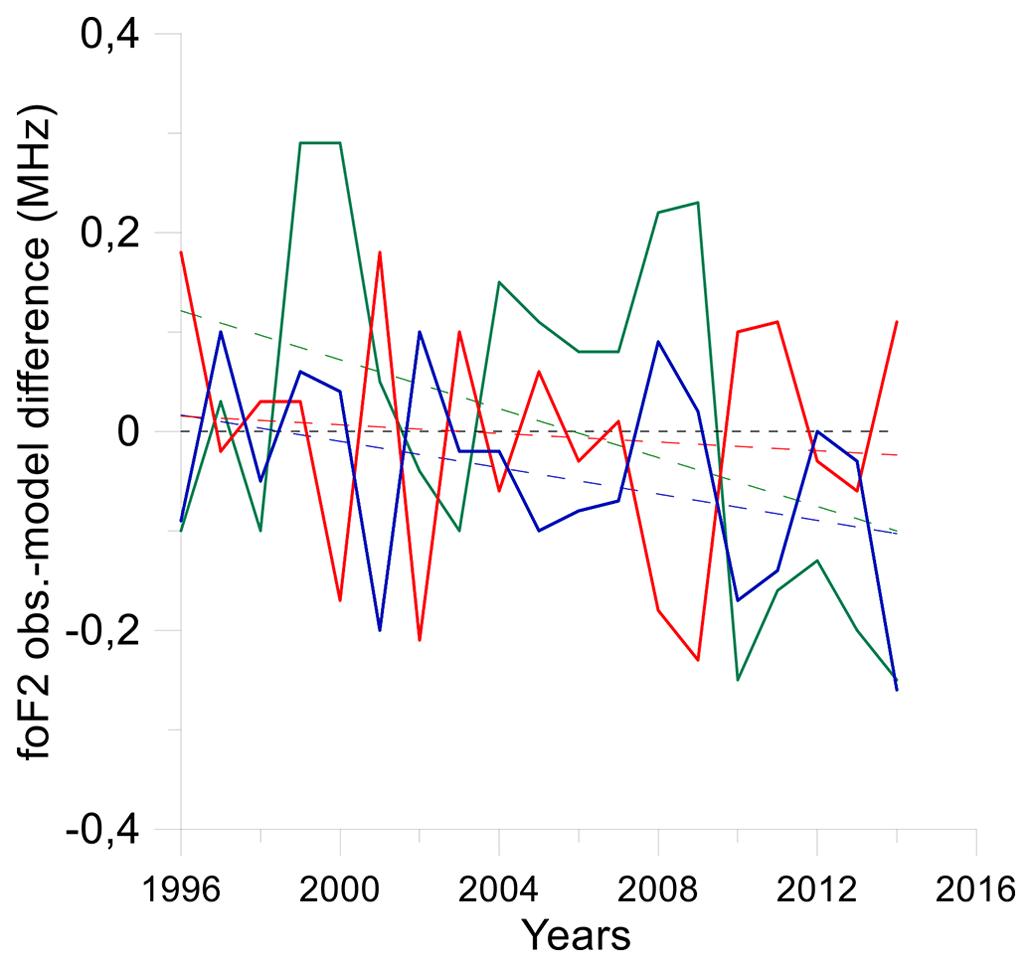
Figure 1Yearly values of foF2 residuals after removing solar influence for Pruhonice, 1996–2014. Green curve: solar-activity proxy F10.7; blue curve: solar proxy F30; red curve: solar proxy Mg II; longer colored dashes: respective linear trends; short horizontal black dashes: zero difference level. A negative difference means smaller observed than model value. After Laštovička (2021b).
The problem of the most suitable solar-activity proxy for ionospheric investigations was treated by Laštovička (2019, 2021a, b). They used yearly average and monthly median foF2 data of three midlatitude European stations – Juliusruh (54.6∘ N, 13.4∘ E), Pruhonice (50.0∘ N, 14.6∘ E), and Rome (41.8∘ N, 12.5∘ E) – and six solar-activity proxies – F10.7, F30, Mg II, He II, sunspot numbers, and the solar H Lyman-α flux – analyzed over two periods, 1976–1995 and 1996–2014. This analysis suggests that F30 and Mg II are the most suitable solar-activity proxies, not the traditionally used proxies F10.7 and sunspot numbers. Preliminary results for yearly foE (critical frequency of the ionospheric E region, corresponding to its electron density maximum), based on data of the Juliusruh and Slough/Chilton (51.7∘ N, 1.3∘ W) stations, favor F10.7. Danilov (2021) reported that the relationship between F10.7 and three other solar-activity proxies – sunspot number, Mg II, and Lyman-α flux – is close in solar cycles 22 and 23 but differs in cycle 24, for which he suggested correction of F10.7 for foF2 long-term investigations.
Danilov and Konstantinova (2020b) estimated foF2 trends of the Juliusruh and Boulder (40.0∘ N, 105.0∘ W) stations until 2018 and found peculiar foF2 trend changes in solar cycle 24. To get a reasonable foF2 trend compared to the previous period, F10.7 has to be corrected with sunspot number and the solar Lyman-α flux values. Danilov and Konstantinova (2020c) found the same problem and the same solution for hmF2.
Huang et al. (2020) claim that due to the seasonal dependence of the relationship between NmF2 (the maximum electron density in the ionosphere located at the maximum of the F2 region) and solar EUV (extreme ultraviolet) irradiance, the application of yearly values (average from monthly average values) to trend calculations may result in both positive and negative biases. For Juliusruh, 1970–2014, they obtained trends of electrons m−3 yr−1 for yearly average values, for monthly average values, and for bias-corrected yearly values. However, all differences between the above trends are within error bars; i.e., they are not statistically significant.
It should be mentioned here that an important problem of some trend calculations may be atmospheric tides. The impact of atmospheric tides via data sampling might be important when the local time of measurement is not fixed or where there are trends in the tides that make the trend dependent on the local time. One more problem is that particularly ionospheric trends might be strongly seasonally and diurnally (local time) dependent up to the change in trend sign, as is demonstrated in Sect. 5; this is not the effect of tides.
Summary
Main progress was made in shedding light on problems related to natural variability, mainly on the critical problem of removal/suppression of the effect of the solar cycle using various solar-activity proxies, and also in specifying problems of solar cycle 24. As concerns data problems, mainly homogeneity of long data series, there are various techniques for how to detect discontinuities and other possible problems which are used, for example, in climatology and meteorology, so no special techniques are needed to be developed for the upper atmosphere. As concerns methodology, we may use methods developed for climatological and meteorological investigations and other available techniques, but as data show, often it is sufficient to use simple or multi-parameter regression because the long-term trend signals and signal-to-noise ratios are often substantially stronger than in the troposphere. On the other hand, the amount of data available in the upper atmosphere is much smaller and data series shorter than those in the troposphere.
Long-term trends in various parameters have been investigated in the mesosphere and lower thermosphere (MLT; altitudes about 50–120 km). The most studied parameter is temperature, but both zonal and meridional winds, minor constituents, noctilucent clouds, water vapor concentration, and some other parameters have been studied as well. We begin the review with observational results of trends in temperature. Many of these studies were based on SABER (Sounding of the Atmosphere using Broadband Emission Radiometry) observations on board the TIMED (Thermosphere Ionosphere Mesosphere Energetics and Dynamics) satellite.
The 17-year-long (2000–2016) midnight spectral OH* airglow measurements at Zvenigorod (56∘ N, 37∘ E) revealed a weak negative trend of mesopause region temperature of K per decade (Perminov et al., 2018).
Continuous Na lidar measurements of nocturnal mesopause region characteristics at Fort Collins (41∘ N, 105∘ W) and Logan (42∘ N, 112∘ W) over 1990–2018 revealed a cooling trend larger than −2 K per decade and a decrease in the wintertime upper-mesopause height (above 97 km) of −450 m per decade and in the lower non-winter mesopause (height below 92 km) of −130 m per decade. WACCM-X (Whole Atmosphere Community Climate Model eXtended) provides similar changes in the mesopause heights caused mainly by cooling and contraction of the stratosphere and lower mesosphere (Yuan et al., 2019).
She et al. (2019) reported results of nighttime temperature measurements by a midlatitude Na lidar over 1990–2017. The height profile of the 28-year-long temperature data trend begins with a weak positive warming at 85 km, continues with cooling at 87 or 88 km with maximal cooling at 92 or 93 km, and turns to a warming trend at 102 or 100 km. The wintertime trend is much cooler than the summertime trend. The lidar temperature trends generally agree with SABER temperatures and within error bars also with LIMA (Leibniz-Institute Middle Atmosphere Model). They also show that data sets longer than two solar cycles are necessary to obtain a reliable long-term trend.
Li et al. (2021) merged middle-atmosphere temperature observations from HALOE (Halogen Occultation Experiment, 1991–2005) and SABER (2002–2019) at 45∘ S–45∘ N. They found stronger mesospheric cooling in the Southern Hemisphere (SH) than in the Northern Hemisphere (NH), which peaks at 60–70 km with a trend of −1.2 K per decade. The temperature trend derived from SABER data only is weaker than that based on merged data by a factor of 1.5, which is consistent with some upper-stratosphere ozone recovery after the mid-1990s.
Venkat Ratnam et al. (2019) merged data on the middle atmosphere over India obtained by various measuring techniques (rockets, HRDI (High Resolution Doppler Imager)/UARS (Upper Atmosphere Research Satellite), HALOE (Halogen Occultation Experiment)/UARS, SABER (Sounding of the Atmosphere using Broadband Emission Radiometry)/TIMED (Thermosphere Ionosphere Mesosphere Energetics Dynamics), and Mesosphere–Stratosphere–Troposphere (MST) radars) over more than 25 years. The observational analysis was accompanied by WACCM-X simulations. They found a significant cooling trend of K per decade between heights of 30 and 80 km. All observed changes are well captured by the WACCM-X simulations if changes in greenhouse gas concentrations are included.
Measurements of OH nightglow rotational temperature spanning 24 years at Davis, Antarctica (68∘ S, 78∘ E), revealed a cooling trend of K per decade (French et al., 2020). The comparison for the trend of the last 14 years with the trend derived from Aura/MLS (Microwave Limb Sounder) at a level of 0.00464 hPa gives very good agreement.
Dalin et al. (2020) reported an update of long-term trends of mesopause temperature in the Moscow region (around 55∘ N). They statistically observed cooling of the summer mesopause region by K per decade and an insignificant and small cooling in winter for the period 2000–2018.
Huang and Mayr (2021) analyzed zonal-mean SABER temperatures over 2002–2014. They found that trends might significantly vary with local time and height in the whole height range of 30–110 km. Figure 2 shows that even for zonal mean temperatures the trends at 00:00, 06:00, 12:00, and 18:00 LT (local time) clearly differ, particularly at 12:00 and 18:00 LT and above about 75 km. However, it is possible that with a longer data series available the differences would be smaller.

Figure 2Temperature trends (K per decade) vs. altitude from 20 to 100 km at 20∘ N (a) and 44∘ N (b). Black: trends based on SABER zonal means over longitude and local time; blue: based on zonal means at 00:00 LT; green: 06:00 LT, red: 12:00 LT, magenta: 18:00 LT. After Huang and Mayr (2021).
Bailey et al. (2021) created temporal series of mesospheric temperatures and pressure altitudes by combining observations from HALOE, SABER, and SOFIE (Solar Occultation for Ice Experiment) for June in the Northern Hemisphere (NH) and December in the Southern Hemisphere (SH) for latitudes 64–70∘ N and S. They found a robust result indicating that the mesosphere generally cools at most heights by 1–2 K per decade in response to the increasing greenhouse gas concentrations, the cooling peaking near 0.03 hPa in the NH and 0.05 hPa in the SH. This cooling results in atmospheric shrinking by 100–200 m per decade. Shrinking results in reduced cooling and eventually heating near 0.005 hPa due to hydrostatic contraction.
Zhao et al. (2020) examined global distribution and changes in monthly average mesopause temperatures based on SABER measurements at latitudes 83∘ S–83∘ N over 2002–2019. They observed cooling at all latitudes ranging from ∼0 to −1.4 K per decade, with a mean value of K per decade and stronger cooling in the SH than in the NH. At high latitudes, the cooling is significant in non-summer seasons; there is no significant trend in summer. They observed the weakest trends at 40–60∘ N and the strongest trends at 60–80∘ S.
Das (2021) examined SABER temperature data for long-term trends over 2003–2019 using the empirical mode decomposition method. He confirmed global cooling of the middle atmosphere and found long-term trends of −0.5 K per decade in the lower mesosphere and −1.0 K per decade in the upper mesosphere. The SH mesopause and NH stratopause exhibit stronger cooling than the opposite hemisphere. The SH mesopause shows stronger cooling over the Indian Ocean.
Zhao et al. (2021) presented another analysis of SABER temperature measurements for 2002–2020 at heights of 20–110 km. The near-global-mean temperature exhibits consistent cooling trends throughout the middle atmosphere ranging from −0.28 up to −0.97 K per decade.
Bizuneh et al. (2022) analyzed long-term mesospheric (60–100 km) variability in temperature and ozone mixing ratio as measured by SABER over 2005–2020 at latitudes 5–15∘ N. They found negative trends in temperature and ozone in the lower mesosphere of −0.85 K per decade and −0.12 ppmv per decade, respectively, and positive trends at 85–100 km of 1.25 K per decade and 0.27 ppmv per decade, respectively. Both temperature and ozone are affected by F10.7, El Niño–Southern Oscillation (ENSO; Niño 3.4 index), and the Quasi-Biennial Oscillation (QBO; QBO30 index).
Mlynczak et al. (2022) used SABER/TIMED observations over 2002–2021 to study the behavior of the MLT region. They found significant cooling and contraction from 2002 to 2019 (solar-cycle minimum) due to a weaker solar cycle and increasing CO2. The MLT thickness between 1 and 10−4 hPa contracted by 1333 m, out of which 342 m can be attributed to increasing CO2. The MLT region sensitivity to CO2 doubling was estimated to be −7.5 K according to the observed temperature trends and CO2 growth rate.
Rayleigh lidar observations at the Observatoire de Haute Provence (44∘ N, 6∘ E), which cover 4 decades, did not reveal any long-term change in mesospheric temperature inversion layers potentially related to climate change (Ardalan et al., 2022). Only an interannual variability with quasi-decadal oscillations was observed.
The observational analyses have been accompanied and supported by model simulation analyses of long-term trends in the MLT region temperatures, which are reported below.
Qian et al. (2019) simulated trends in mesospheric temperature and winds with WACCM-X and compared them with winds observed at Collm over 1980–2014. They found a global temperature trend in the mesosphere to be negative, in line with observations, reaching a maximum of about −1 K per decade in the middle and lower mesosphere (∼55–65 km). The temperature trend becomes near-zero or even slightly positive in the summer upper mesosphere. This is likely due to dynamical effects associated with the mesospheric meridional circulation, which is driven by the breaking of upward-propagating gravity waves (Qian et al., 2019).
Kuilman et al. (2020) simulated the impact of CO2 doubling on the middle atmosphere with WACCM; they found the direct mesospheric cooling to reach up to 15 K.
Ramesh et al. (2020b) simulated long-term (1850–2014) variability in temperature and zonal wind with WACCM-6. They confirmed CO2 and ozone-depleting substances (ODSs) to be the main drivers of the observed cooling of the middle atmosphere. The simulated cooling was stronger in the lower mesosphere than at higher mesospheric levels.
Another important parameter is wind. Trends in winds, particularly in zonal wind, were studied with both observations and model simulations.
Venkat Ratnam et al. (2019) carefully merged data on the middle atmosphere (stratosphere, mesosphere, and lower thermosphere) over India obtained by various measuring techniques (rockets, HRDI/UARS, HALOE/UARS, SABER/TIMED, and MST radars) over more than 25 years. The eastward zonal wind trend was large, about −5 m s−1 per decade, but statistically significant only at 70–80 km, which resulted in a change from a strong eastward wind in the 1970s to a weak westward wind in the last decade; no significant trend was found in meridional wind. All observed changes are well captured by the WACCM-X simulations if changes in greenhouse gas concentrations are included.
Meteor radar winds measured at Andenes (69.3∘ N, 16∘ E), Juliusruh (54.6∘ N, 13.4∘ E), and Tavistock (43.3∘ N, 80.8∘ W) over 2002–2018 revealed annual wind tendency toward the south and west (up to 3 m s−1 per decade) for Andenes but slight opposite to negligible tendencies at midlatitudes (Wilhelm et al., 2019).
Vincent et al. (2019) derived vertical wind velocities from the divergence of mean meridional wind measured by MF (medium frequency) radar above Davis, Antarctica (69∘ S, 78∘ E), over 1994–2018 in the 3 weeks just after summer solstice. The estimated vertical velocity peak values varied between 2 and 6 cm s−1 with significant interannual variability. These peak values did not exhibit a significant long-term change, but the height of wind maximum displayed a statistically significant long-term decrease of about −0.6 km per decade.
Qian et al. (2019) simulated with WACCM-X trends in mesospheric temperature and winds and compared them with winds observed at Collm over 1980–2014. They found, as Fig. 3 shows, that trends in winds near an altitude of 90 km reveal a dynamical pattern with regionally both positive and negative values within about ±5 m s−1 per decade, which indicates predominant control by dynamics. Figure 3 illustrates how complex trends are in winds and how difficult it is to investigate them.

Figure 3Average monthly mean zonal wind at 0.001 hPa (∼90 km) for March, June, September, and December, simulated by WACCM-X for the period of 2000–2014 (top row). The corresponding zonal wind trends (middle row). The corresponding solar-irradiance effect on the zonal winds (lower row). After Qian et al. (2019).
Kogure et al. (2022) focused on mechanisms of the thermospheric zonal-mean wind response to doubling the CO2 concentration based on simulations from the GAIA (Ground-to-topside model of Atmosphere and Ionosphere for Aeronomy) model. The pattern is very complex; three main forces – ion drag, molecular viscosity, and meridional pressure gradient – strongly attenuate each other.
Atmospheric waves, namely gravity waves, planetary waves and tides, are a very important vertical coupling mechanism between the upper atmosphere and ionosphere, and the lower atmosphere below. Unfortunately there was little activity in investigating trends in wave activity.
Meteor radar winds measured at Andenes (69.3∘ N, 16∘ E), Juliusruh (54.6∘ N, 13.4∘ E) and Tavistock (43.3∘ N, 80.8∘ W) over 2002–2018 revealed no significant trend in diurnal tides and changes in semidiurnal tide, which differ according to altitude and latitude (Wilhelm et al., 2019).
The WACCM6-simulated trends of the migrating diurnal tide amplitude in the MLT region (0.0001–0.01 hPa) for the period 1850–2014. Trends were found to be positive, mainly due to the increasing concentration of CO2 with some contribution of the trend of ENSO (Ramesh et al., 2020a).
Ramesh and Smith (2021) used WACCM6 simulations over 1850–2014 and found an increasing non-migrating diurnal tide in the MLT region (0.0001–0.01 hPa) in temperature and zonal and meridional winds, particularly at low and equatorial latitudes, predominantly due to the increasing concentration of CO2.
New results were obtained in studies of long-term trends in the MLT region composition, namely in CO2 and water vapor, and related trends in noctilucent clouds, also called polar mesospheric clouds when they are observed from above by satellites.
Rezac et al. (2018) analyzed long-term trends of CO2 based on direct SABER measurements. They found that below 90 km the CO2 trends statistically do not differ from the surface/tropospheric CO2 trends, in agreement with model simulations, whereas above 90 km up to 110 km (top height of measurements) the CO2 trends are slightly higher but less than provided by previous analyses. This important study closed several years of discussions on the satellite-based trend of CO2, which was originally reported to be higher than near the surface.
Yu et al. (2022) studied water vapor evolution in the tropical middle atmosphere with the merged data set of satellite observations between 1993 and 2020 and SD-WACCM (WACCM6 with specified dynamics) simulations over 1980–2020. They found a relatively weak trend of 0.1 ppmv per decade in observations and no trend in simulations. Simulations revealed periods of increasing as well as decreasing mesospheric water vapor due to non-linear changes in methane emissions and sometimes irregular changes in the tropical tropopause temperature.
Nedoluha et al. (2022) examined measurements of mesospheric water vapor by the Water Vapor Millimeter-wave Spectrometer (WVMS) instruments at three stations in California, Hawaii, and New Zealand from 1992 to 2021 and compared them with measurements on board satellites by HALOE, SABER, and Aura/MLS. Differences between ground-based and satellite trends vary within ∼ 3 % per decade. This uncertainty is comparable with trends of mesospheric water vapor since the early 1990s. The increase in CH4 concentration over the last 30 years should increase H2O mixing ratio by ∼ 4 %, which corresponds to a trend of 1.3 % per decade. Such a trend is within the range of trends and their uncertainties derived from measurements of other WVMS instruments.
Yue et al. (2019) report an increase in water vapor concentration in the mesosphere over 2002–2018 of 0.1–0.2 ppmv per decade according to SABER measurements and 0.2–0.3 ppmv per decade according to Aura/MLS measurements. The trend is somewhat stronger in the lower and upper mesosphere. WACCM simulations provide the same trend of water vapor as observations in the lower mesosphere. The origin of water vapor trend is partially dissociation of methane (mainly above 65 km) and partially transport of water vapor from below.
On the other hand, measurements of the mesospheric water vapor concentration by the radiometer MIAWARA (Middle Atmospheric WAter vapor RAdiometer) in Zimmerwald (46.88∘ N, 7.46∘ E) in Switzerland over 2007–2018 displayed a significant decrease in water vapor concentration with a rate of ppmv per decade at heights of 61–72 km (Lainer et al., 2019). The authors were not able to give an explanation for the origin of the detected water vapor decline.
A 138-year-long model simulation of the impact of increasing concentration of CO2 and methane near 83 km altitude revealed a substantial increase in the noctilucent cloud (NLC) brightness due to a ∼ 40 % increase in water vapor induced by increasing methane concentration (Lübken et al., 2018). This increase is qualitatively consistent with polar mesospheric cloud observations by satellites. The origin of the water vapor trend is partially dissociation of methane (mainly above 65 km) and partially transport of water vapor from below.
Lübken et al. (2021) analyzed long-term trends in mesospheric ice layers derived from simulations with LIMA and MIMAS (Mesospheric Ice Microphysics And tranSport model) over the period of 1871–2008 for middle (58∘ N), high (69∘ N), and Arctic (78∘ N) latitudes. Increases in ice particle radii and NLC brightness with time are mainly caused by an enhancement of water vapor. The negative trend of NLC heights is primarily caused by CO2-induced cooling at lower heights.
Dalin et al. (2020) reported an update of long-term trends in noctilucent clouds in the Moscow region around 55∘ N. Trends in noctilucent clouds over 1968–2018 were small and insignificant, in agreement with other observations from comparable latitudes.
Long-term trends have also been studied in other parameters of the mesosphere and lower thermosphere, in airglow, polar mesospheric summer echoes, and summer length (defined using spring and autumn wind reversal) in the MLT region.
Huang (2018) used the 55-year-long series of results of simulations by two models focused on examining the effect of increasing CO2 concentration on airglow intensity, volume emission ratio (VER), and VER peak height. He found weak and opposite linear trends of airglow intensities of OH(8,3), O(0,1), and O(1S) spectral lines and of VER with increasing CO2, whereas the VER peak height is strongly correlated and out of phase with geomagnetic activity.
Observations of mesopause airglow emissions of O2(A 0-1) and OH (6-2) at Zvenigorod (55.4∘ N, 36.5∘ E) over 2000–2019 provided a trend of average yearly emissions of % per decade and % per decade, respectively (Perminov et al., 2021), which is surprisingly strong trend.
Dalin et al. (2020) reported an update of long-term trends in airglow emission intensity in the Moscow region. They found statistically significant negative trends in the intensities of O2A(0-1) and OH (6-2) airglows in both summer and winter for the period 2000–2018.
Based on radar observations at Andoya (69.5∘ N, 16.7∘ E) over 1994–2020, Latteck et al. (2021) obtained after eliminating the effects of solar and geomagnetic activity a polar mesospheric summer echo trend of 3.2 % per decade, which might be related to the observed negative trend of mesospheric temperatures at polar latitudes.
Mesospheric wind measurements by specular meteor radars and partial-reflection radars over northern Germany (∼ 54∘ N) and northern Norway (∼ 69∘ N) between 2004–2020 using two definitions of summer length provided a positive trend of summer length for the mesosphere only but no clear trend for the whole MLT region. The 31-year midlatitude partial-reflection radar data indicate a break point and non-uniform trend of summer length, i.e., a slight negative trend from 1990–2008, a break in 2008, and a positive trend from 2008–2020 (Jaen et al., 2022).
Simulations with NASA's (National Atmospheric and Space Administration) E2.2-AP model reveal an impact of CO2 on the quasi-biennial oscillation (QBO). The increasing concentration of CO2 results in a reduction in the QBO period (Dalla Santa et al., 2021). QBO is a stratospheric phenomenon but with an impact on the mesosphere.
Summary
The mesosphere and lower thermosphere were the most actively studied regions of the upper atmosphere and ionosphere system in the past 5 years from the point of view of long-term trends. The most studied parameter was temperature due to both its importance (the primary direct effect of increasing concentration of CO2 at heights above ∼ 50 km is radiative cooling) and availability of both ground-based and satellite-based data as well as model simulations. The general pattern is cooling, particularly in the mesosphere, but various observations are only mostly but not fully consistent, maybe partially due to insufficient length of the data series used; She et al. (2019) claim that data sets longer than two solar cycles are necessary to obtain a reliable long-term trend. Huang and Mayr (2021) found that trends might significantly vary with local time and height in the whole height range of 30–110 km, but they studied data series that are only 13 years long. Also model simulations provide general cooling, even though the WACCM simulations by Qian et al. (2019) indicate that the temperature trend becomes near-zero or even slightly positive in the summer upper mesosphere, likely due to dynamic effects (winds and atmospheric wave activity). The results of temperature trends are generally consistent with older results. It should be mentioned that temperature trends are also affected by the stratospheric ozone behavior, which was highly non-linear due to a change after the mid-1990s from relatively rapid decline to much weaker decline, stagnation, or recovery (depending on region and altitude). In summary, it is clear that long-term trends in the MLT temperature are now better known and understood than before 2018; our knowledge broadened, and it is more detailed; e.g., trends are now better quantified, model-derived trends are in agreement with observational trends, and some hemispheric asymmetry of temperature trends was found.
Dynamical parameters, such as winds and atmospheric waves, play a critical role in the MLT region. Here the trend pattern is much more complex. Observational data indicate different wind trends up to the sign of the trend in different geographic regions (e.g., Wilhelm et al., 2019). Simulations (Qian et al., 2019) show that trends in winds reveal a dynamical pattern with both positive and negative values. A limited activity in the area of atmospheric waves was focused on tides in 2018–2022. Meteor radar wind data from high/middle latitudes revealed no significant trend in diurnal tides and changes in semidiurnal tide, which differ according to altitude and latitude (Wilhelm et al., 2019). On the other hand simulations with WACCM6 provide positive trends for both migrating and non-migrating diurnal tides. Trends in dynamical parameters are not well understood, which is the key problem of trend studies in the upper atmosphere. They seem to be substantially regionally dependent.
Another group of parameters is composed of CO2, water vapor, and noctilucent clouds. Rezac et al. (2018) finally solved contradictions about evaluations of satellite measurements of concentration of CO2, which is the result of principal importance. It was found that the CO2 concentration trends in the mesosphere (below 90 km) do not differ statistically from trends at the surface, even though they appear to be slightly larger above 90 km. Water vapor trends in the mesosphere are generally positive; it is only in the equatorial region that trends are very little or near-zero. The only exception is radiometer measurements in Switzerland, with a significant negative trend at heights of 61–72 km with an unknown explanation. As for noctilucent clouds, recent results confirm positive trends, which weaken with decreasing latitude. This trend is mainly due to the increase in water vapor concentration. Their height is slightly decreasing primarily due to mesospheric shrinking due to CO2-induced cooling at lower heights.
Long-term trends were also studied in other parameters. Airglow intensities in different spectral lines have different and even opposite trends, even though negative trends dominate. The polar mesospheric summer echo trend was found to be positive, which might be related to the observed negative trend of mesospheric temperatures at polar latitudes. Midlatitude partial-reflection radar data indicate a break point and non-uniform trend of mesospheric summer length.
The research activity in the field of thermospheric long-term trends has been moderate. Out of the five papers cited below, three dealt with long-term trends in thermospheric density.
Weng et al. (2020) applied the machine-learning method to satellite drag data from a broad range of altitudes in the thermosphere to search for long-term trends in thermospheric density. Their trend estimates range from −1.5 % per decade to −2.0 % per decade between 250 and 575 km without any clear dependence on solar activity. They use S10.7 instead of F10.7 to represent solar activity. Their model better captures thermospheric density during the deep solar minimum 2008–2009 than previous empirical models.
Mlynczak et al. (2022) used SABER/TIMED observations over 2002–2021 to study the behavior of the MLT region (heights of ∼ 48–105 km, low and middle latitudes). They found significant cooling and contraction from 2002 to 2019 (solar-cycle minimum) due to weaker solar cycle and increasing CO2. The cooling and contraction of the MLT region contribute to decreasing thermospheric densities in LEO (low Earth orbit) satellite orbits, resulting in increasing concentration of dangerous space debris.
WACCM-X global simulation of the impact of increasing CO2 concentration on thermospheric density under low-solar-activity conditions reveals a 27 %–30 % decrease in atmospheric density at 400 km with respect to year 2000 levels if the Paris Agreement surface warming limit of 1.5 ∘C is reached. This thermospheric density decrease will result in a satellite and space debris orbital lifetime that is longer by 30 %, with a consequent higher probability of dangerous satellite collisions with space debris (Brown et al., 2021). However, their neutral density trend at low solar activity is much higher than under medium- and high-solar-activity conditions, and it is almost 3 times as high as the recent observational trends (e.g., Weng et al., 2020).
Liu et al. (2020) use GAIA model simulations to study the response of the thermosphere at heights of 100–400 km to CO2 doubling. They found that the thermosphere will cool by 10 K, more near solstices than near equinoxes and more at the summer pole than at the winter pole. The meridional circulation shifts downward and strongly increases by 5–15 m s−1. Semidiurnal tides are reduced by 40 %–60 % in the whole thermosphere.
Perrone and Mikhailov (2019) inferred the atomic oxygen column content n[O]col in June from June monthly medians of foF1 (critical frequency of F1 layer, corresponding to its maximum electron density, height ∼ 200 km) and foF2 (heights of 250–300 km) of NH stations Rome (41.8∘ N, 12.5∘ E), Juliusruh (54.6∘ N, 13.4∘ E), Sodankylä (67.4∘ N, 26.6∘ E), and Boulder (40.0∘ N, 105.0∘ W) for six solar cycles (1958–2017). A total of 93% of total variance of n[O]col is explained by the solar and geomagnetic activity. The linear trend for three midlatitude stations is negative but statistically insignificant, whereas Sodankylä reveals a statistically significant negative trend of n[O]col, but this trend might be an artifact due to not considering particle precipitation.
Summary
The observed negative trend of thermospheric density of about −2 % per decade near 400 km continues without any evidence of clear dependence on solar activity, which is not consistent with model simulations under low-solar-activity conditions. The decrease in thermospheric density will result in increasing concentration of dangerous space debris in LEO satellite orbits. Complex GAIA model simulations of trends in many thermospheric parameters predict among other things a downward shift and acceleration of meridional circulation and substantial reduction in semidiurnal tides; neither has yet been studied observationally. Perrone and Mikhailov (2019) inferred negative trends of the atomic oxygen column content in June, but their method might be questioned.
Research activity in the field of the ionosphere has been more intense than in the thermosphere. It has focused on the F2 region, particularly on foF2 trends due to both the importance of foF2 and availability of the longest and relatively reliable data sets. Some activity was also in the E-region ionosphere trend area. The first trend results were published for electron density in the topside ionosphere. On the other hand, there was little progress in the D-region trends since the review by Laštovička and Bremer (2004) and no activity in the previous 5 years.
Danilov and Konstantinova (2018) analyzed long-term trends in foE (typical heights of ∼ 110–115 km) for the Juliusruh (54.6∘ N, 13.4∘ E) and Slough/Chilton stations over the period 1960–2010; they found trends of −0.12 and −0.05 MHz per decade, respectively, for yearly values and negative trends as well as for all months for the period after 1980.
Danilov and Konstantinova (2019) analyzed long-term changes in foE from the Juliusruh, Slough/Chilton, Rome (41.8∘ N, 12.5∘ E), Moscow (55.5∘ N, 37.3∘ E), and Wakkanai (45.2∘ N, 145.7∘ E) stations over the period 1960–2010. They found strong local-time dependence of the foE trend for Juliusruh, as shown in Fig. 4, with positive trends in the morning sector, no trend at 11:00 LT, and negative and stronger trends in the afternoon. The dependence of the foE trend on LT is much weaker for Rome (lower latitude). Seasonally the trends reach a maximum in December–January and a minimum in July–August for Juliusruh (Fig. 4). The magnitude of foE trends clearly depends on geomagnetic latitude (Juliusruh and Slough/Chilton: 54∘ N; Moscow: 51∘ N; Rome: 42∘ N; Wakkanai: 36∘ N); the trend weakens with decreasing latitude. This finding according to Danilov and Konstantinova (2019) provides evidence supporting the impact of meridional transport of NO from the auroral zone on the observed trends in foE.

Figure 4Seasonal variations in the trend slope/coefficient of foE for various LT moments for the Juliusruh station (54.6∘ N, 13.4∘ E). After Danilov and Konstantinova (2019).
Givishvili and Leshchenko (2022) used data of Moscow and five Japanese stations to search for a long-term trend in the E-region response to solar flares over 1969–2015. From their analysis they derived the stable long-term increase in the ratio of ionization rates in the E region (qx – soft X-ray ionization rate; qEUV – solar EUV ionization rate); the ratio since 1969 approximately doubled in 2015. The increase was continuous and independent of solar cycle, season, and latitude. Observations at Moscow spanning 74 years provide a small but insignificant increase in foE and a relatively large and significant decrease in h'E (apparent height of the E-layer maximum).
The first results of long-term trends in the topside ionosphere based on DMSP (Defense Meteorological Satellite Program) satellite data over 1995–2017 were reported by Cai et al. (2019). They found the electron density trend near 860 km around 18:00 MLT (magnetic local time) to have a mean magnitude ranging from −2 % per decade to +2 % per decade with a clear seasonal, latitudinal, and longitudinal variation. The TIE (Thermosphere–Ionosphere–Electrodynamics) GCM (general circulation model)-simulated trends at 500 km have a similar geographic distribution at 18:00 MLT. Simulations also suggest that the predominant electron density trend driver at 500 km is the secular change in the Earth's magnetic field.
Zhou et al. (2022) investigated the impact of increasing anthropogenic emissions on the occurrence of equatorial plasma bubbles (EPBs) via simulation of the growth rate of the Rayleigh–Taylor instability, which is closely related to EPB generation. They used the Global Coupled Ionosphere–Thermosphere–Electrodynamics Model of the Institute of Geology and Geophysics, Chinese Academy of Sciences. With increasing CO2 concentration the growth rate significantly increases at low altitudes below about 260 km, decreases at high altitudes above about 320 km, and between 260 and 320 km increases (decreases) before (after) midnight, indicating a possible impact on radio communication systems. These changes are caused by gravity and the electrodynamic term, not by neutral wind.
Zhang et al. (2018) found that the results of Perrone and Mikhailov (2017; PM17) for exospheric temperature, which were based solely on foF1 measurements, were flawed and quantitatively unlikely. They also showed that the conclusions of PM17 on long-term analysis of ion temperatures derived from the incoherent scatter radar measurements are incorrect, partly due to misunderstanding of the nature of the incoherent scatter radar measuring process.
The remaining papers deal with long-term trends in the F2 region, mainly in foF2 but partly also in hmF2.
An analysis of a 70-year-long homogenized series (1947–2017) of observations of ionosondes at Wuhan (30∘ N, central China) by Yue et al. (2018) found a weak but statistically significant average negative trend in foF2, −0.021 MHz per decade, which varied with local time from negative to slightly positive. The observed trends are attributed primarily to the secular change in the Earth's magnetic field, with CO2 being the secondary important driver. As for hmF2, the average trend is −1.06 km per decade; the roles of CO2 and Earth's magnetic field in this trend are comparable (Yue et al., 2018).
Sharan and Kumar (2021) examined long-term foF2 variations from SH stations Hobart, Canberra (35.3∘ S, 149.1∘ E), and Christchurch (43.5∘ S, 172.6∘ E) over 1947–2006. They found a decrease in foF2 of 0.1–0.4 MHz per five solar cycles mainly due to increasing concentration of CO2; the midday trends were more significant and agreed better with model-inferred expectations than midnight trends.
When the solar cycle 24 is included in nighttime foF2 long-term trends for the Wakkanai (45.4∘ N, 141.7∘ E) and Kokubunji (35.7∘ N, 139.5∘ E) stations, the trends become less negative, likely due to application of F10.7 as a solar-activity proxy (De Haro Barbas et al., 2020). The trend weakening is less pronounced when Mg II is used as a solar-activity proxy instead of F10.7.
Danilov and Konstantinova (2020c) found for Juliusruh that the pronounced negative trends of hmF2 and foF2 persisted until 2002–2003; then they were followed by a vague period with chaotic changes, and in the most recent years a negative trend appeared again.
Sergeenko (2021) analyzed significant deviations (> 20 %) of foF2 (ΔfoF2) from the 10 d median for the Moscow (55.5∘ N, 37.3∘ E), Slough/Chilton (51.5∘ N, 01∘ W), and Hobart (42.9∘ S, 147.3∘ E) stations for the period 1948–2010. They found that the maximum amplitudes of positive ΔfoF2 increased since the early 1980s at all stations in winter and, except in Moscow, also in summer, whereas for negative ΔfoF2 there was no change in Chilton and Hobart and some increase in Moscow (particularly in summer). The increasing trend in positive ΔfoF2 is likely related to changes in the thermospheric wind system (Sergeenko, 2021).
Summary
Significant progress was reached in long-term trends in the E-region ionosphere, namely in foE. These trends were found to depend principally on local time up to their sign; this dependence is strong at European high midlatitudes but much less pronounced at European low midlatitudes, and it is stronger in winter than in summer. Trends in foE also weaken with decreasing geomagnetic latitude of station.
In the ionospheric F2 region very long data series (starting in 1947) of foF2 in the NH as well as the SH revealed very weak but statistically significant negative trends. Some problems with foF2 and hmF2 trends were indicated in solar cycle 24 (e.g., De Haro Barbas et al., 2022) and around the solar-cycle minimum (e.g., Danilov and Konstantinova, 2020c).
First results of long-term trends in the topside ionosphere electron densities (trends ranging from −2 % per decade to +2 % per decade at 840 km) and in the equatorial plasma bubbles (height-dependent sign of trends) were reported.
The role of secular change in the Earth's magnetic field in long-term trends in the F2 region has also been studied, but these results are reported in Sect. 7. The results of selection of the optimum solar-activity proxies for F2 region trend studies are reported in Sect. 2.
Solomon et al. (2019) realized with WACCM-X the first global simulation of changes in temperature excited by anthropogenic trace gases simultaneously from the surface to the base of the exosphere. They found that the anthropogenic cooling begins in the lower stratosphere, and it becomes dramatic, almost −2 K per decade, for the global-mean and zonal-mean temperature in the thermosphere. Only near the mesopause (∼ 85–90 km) does the cooling approach zero values. This pattern qualitatively agrees with observations. The temperature trend in the thermosphere is somewhat stronger in the solar-cycle minimum compared to the solar-cycle-maximum conditions, likely due to the stronger solar-cycle variation in NO and O(3P) infrared irradiance compared to that of CO2, which results in a relatively larger role of CO2 under solar-activity-minimum conditions.
Cnossen (2022) used WACCM-X to simulate climate change in the upper atmosphere (90–500 km) for the period 1950–2070 with moderate-emission scenario SSP2-4.5 (Shared Socio-economic Pathway), secular change in the Earth's magnetic field, and reasonable solar radiative and particle forcing in order to get the climate projection into the 21st century. The obtained trends of thermospheric temperature (cooling) and density (reduction) are twice as large in 2015–2070 compared to the period 1950–2007 due to the more rapid absolute increase in CO2 concentration. Trends in ionospheric parameters also become substantially stronger. However, they display considerable spatial variability due to the secular change in the Earth's magnetic field. The strongest ionospheric changes are expected in the region of 50∘ S–20∘ N, 90–0∘ W.
Yue et al. (2022) expanded simulations of the ionosphere over the whole Holocene (9455 BCE–2015 CE) for the first time with the Global Coupled Ionosphere–Thermosphere–Electrodynamics Model of the Chinese Institute of Geology and Geophysics driven by realistic geomagnetic field, CO2 levels, and solar activity. They found that oscillations of the global-mean ionospheric profile are characterized by effects of geomagnetic field, decrease (increase) in electron density above (below) ∼ 200 km due to increasing CO2 concentration, and violent oscillations in phase with solar activity, the corresponding contributions to overall variability being about 20 %, 20 %, and 60 %, respectively. The CO2 effect becomes non-negligible and significant after ∼ 1800 CE. The increase in CO2 by 400 ppmv resulted in a simulated decrease in foF2 of 1.2 MHz, in hmF2 of 34 km, and in TEC of 4 TECU (total electron content units).
Garcia et al. (2019) simulated middle-atmosphere temperature trends in the 20th and 21st centuries with WACCM. They investigated bi-decadal changes in temperature trend profiles with the RCP 6.0 scenario of the greenhouse gas concentration evolution and found the biggest change between 1975–1995 and 1995–2015, which is attributed to loss and recovery of stratospheric ozone due to changing emissions of anthropogenic halogens. After 2015 the development of profile of temperature trends is controlled mainly by non-ODS greenhouse gases.
Summary
Trends in temperature in the whole atmosphere from the surface to the exosphere were simultaneously simulated for the first time; in individual layers they reasonably agree with other results. The simulation confirmed the observed height-dependent pattern of trends. Very-long-period simulations of the middle atmosphere, thermosphere, and ionosphere confirmed acceleration of the trends during the last several decades, specified the role of ozone-depleting substances, and provided the first information about possible trends over the whole Holocene.
The increasing concentration of greenhouse gases (GHGs; mainly CO2) is not the only driver of long-term trends in the upper atmosphere (e.g., Laštovička, 2017). At present the effect of secular change in Earth's magnetic field and anthropogenic changes in stratospheric ozone are considered to be the most important additional trend drivers in the ionosphere–thermosphere–mesosphere system. Other drivers' roles are also discussed, e.g., geomagnetic activity, atmospheric waves coming from below, or water vapor (only in the mesosphere). Solar activity also changes on long-term scales, but because we need to remove the solar-cycle effect from (particularly ionospheric) data before calculating trends, the solar-activity effect is largely removed from trend calculations. Let us start with the secular change in magnetic field because its effects were relatively broadly studied in the period 2018–2022.
Cnossen (2020) performed a long-term (1950–2015) simulation of the upper atmosphere with WACCM-X with realistic variation in solar and geomagnetic activity, changes in the main magnetic field, and trace gas emissions including CO2. The results confirm that CO2 is the main driver of trends in thermospheric temperature and density, even though at high magnetic latitudes the secular change in geomagnetic field also plays a role, particularly in the NH. Spatial patterns of trends in hmF2, NmF2, and TEC indicate the superposition of the effects of CO2 and secular change in geomagnetic field, the latter being dominant at about 50∘ S–20∘ N, 60∘ W–20∘ E. This longitudinal sector experiences the largest change in the magnetic equator position (e.g., Cnossen, 2020).
Qian et al. (2021) simulated long-term trends in the upper atmosphere using WACCM-X. They found that trends caused by both the secular change in geomagnetic field and the increasing concentration of CO2 exhibit significant latitudinal and longitudinal variability, which was not expected for CO2. Thermospheric trends in density and temperature are quite predominantly driven by greenhouse gases (GHGs); the secular change in geomagnetic field plays some role in temperature trends at 120∘ W–20∘ E. In this longitudinal sector, the secular change in geomagnetic field plays a comparable role to GHGs in trends in hmF2, NmF2, and Te (electron temperature) as well as in Ti (ion temperature) above 320 km, while below 320 km the Ti trend is dominated by GHGs. Figure 5 shows the changes in neutral density, Tn (neutral temperature), Te, and Ti from the 1960s to the 2010s. The neutral temperature and density change is clearly dominated by GHGs, whereas in Te and Ti in some regions the effect of the secular change in magnetic field plays the dominant role. The secular change in geomagnetic field is an important driver in the 120∘ W–20∘ E sector,but it excites locally both positive and negative trends; consequently, in global average trends, its contribution is negligible.
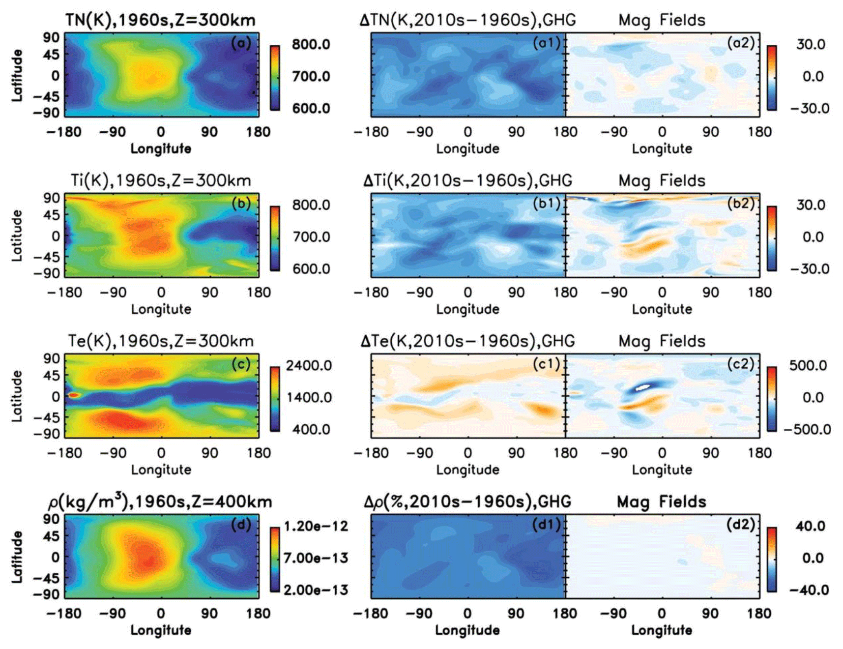
Figure 5Left panels show the global distributions of neutral temperature Tn at 300 km, ion temperature Ti at 300 km, electron temperature Te at 400 km, and neutral density ρ at 400 km in the 1960s. Right panels show changes in global distributions of these four parameters from the 1960s to the 2010s separately for the effect of greenhouse gases (GHGs; in the thermosphere essentially CO2; left part) and of the secular change in the Earth's magnetic field (right part). After Qian et al. (2021).
Simulations with the TIE GCM (Cai et al., 2019) suggest that the predominant electron density trend driver at 500 km is the secular change in the Earth's magnetic field.
During the next 50 years the dipole momentum of the Earth's magnetic field is predicted to decrease by ∼ 3.5 %; the South Atlantic magnetic anomaly will expand, deepen, and drift westward; and magnetic dip poles will also move, which according to simulations with the TIE GCM will have an impact on the thermosphere–ionosphere changes from 2015 to 2065 (Cnossen and Maute, 2020). The global-mean thermospheric density should slightly increase by ∼ 1 % on average and by up to 2 % under magnetically disturbed conditions (Kp ≥ 4), particularly in the SH. Global TEC should change in the range of −3 % to +4 % depending on season and UT, but regional changes may be up to ±35 % at 45∘ S–45∘ N, 110∘ W–0∘ W, during daytime, mainly due to changes in the vertical E × B drift (the vector product of electric and magnetic field is a plasma drift perpendicular to them). The equatorial ionization anomaly will weaken in the ∼ 105–60∘ W sector. The predicted changes in neutral density are very small compared to effects of other trend drivers (mainly CO2), but the predicted changes in TEC might be regionally substantial.
As concerns observational results, Yue et al. (2018) found a weak but statistically significant average negative trend in foF2 from 70 years of data at Wuhan (central China), which they attributed primarily to the secular change in the Earth's magnetic field, with CO2 being the secondary important driver.
Anther discussed topic is the impact of geomagnetic activity on CO2-driven trends in the thermosphere and ionosphere. One paper dealt with long-term changes in NO radiative cooling of the thermosphere.
Liu et al. (2021) used the GAIA model to simulate the impact of geomagnetic activity on CO2-driven trends in the thermosphere and ionosphere. They found that the thermospheric density is the most robust indicator of the effect of CO2. The geomagnetic activity can either weaken or strengthen CO2-driven trends in hmF2 and NmF2 depending on time and latitude. There is interdependency between forcing by CO2 and by geomagnetic activity; the efficiency of CO2 forcing is higher under low geomagnetic-activity forcing than under high levels of geomagnetic-activity forcing, and under conditions of high CO2 concentration the geomagnetic forcing is more efficient.
Chen et al. (2022) found that the geomagnetic-activity-induced long-term change in foF2 is seasonally discrepant. With the long-term increase in geomagnetic activity, foF2 increases in winter, while it decreases in summer at middle and low latitudes; foF2 decreases at higher latitudes, whereas it increases with decreasing latitude during equinoxes. The linear trend component is dominated by a long-term decreasing trend, which is in line with the increasing greenhouse gas concentration. The geomagnetic activity in the most recent decades has a decreasing trend, which has to be considered when the linear trend of foF2 is calculated to estimate the impact of greenhouse gases.
Lin and Deng (2019) studied the role of NO in the climatology of global energy budget and found that from 1982 to 2013 the decadal change in NO cooling reached ∼ 25 % of the change in total heating in the thermosphere below 150 km (its importance decreases with increasing height) based on simulations with the Global Ionosphere–Thermosphere Model (GITM; simulations were run for constant CO2). However, the decadal change in NO cooling was mainly due to decreasing solar (F10.7) and geomagnetic (Ap) activities.
Summary
The main activity focused on the role of the secular change in the main magnetic field of Earth. Model simulations show that its role in long-term trends is most important (comparable to or even higher than the role of GHGs) in ionospheric parameters hmF2, foF2, TEC (total electron content), electron temperature, and partly ion temperature in the region of about 50∘ S–20∘ N, 20∘ E–110∘ W (various simulations provide a somewhat different longitudinal range), while its role in neutral atmosphere, density and temperature is much smaller, almost negligible. In global average trends, however, the role of secular change in magnetic field is negligible even in ionospheric parameters; it excites locally both positive and negative trends (Qian et al., 2021). On the other hand, trends in electron density well in the topside ionosphere (∼ 500–850 km) appear to be controlled by the secular change in geomagnetic field.
Model simulations by Liu et al. (2021) reveal that the geomagnetic activity, another potential driver of long-term trends particularly in the ionosphere, can either weaken or strengthen CO2-driven trends in hmF2 and NmF2 depending on time and latitude.
This article reviews the progress in long-term trends in the mesosphere–thermosphere–ionosphere system reached over the period 2018–2022. Overall this progress may be considered significant. The most active research was reached in the area of trends in the mesosphere and lower thermosphere (MLT). Research areas of problems in trend calculations, global modeling, and non-CO2 drivers of long-term trends have also been reviewed. The main results are as follows.
Trends in the MLT region were relatively broadly studied. The contradictions about long-term trends of concentration of CO2 derived from satellite measurements were finally solved, which is the result of principal importance. It was found that the CO2 concentration trends in the MLT region below 90 km do not differ statistically from trends at the surface, even though they appear to be slightly larger at heights above 90 km. The most studied parameter was temperature. Huang and Mayr (2021) found that trends might significantly vary with local time and height in the whole height range of 30–110 km, but they studied data series that were only 13 years long. However, She et al. (2019) claim that data sets longer than two solar cycles are necessary to obtain a reliable long-term temperature trend. Model simulations confirm general cooling, even though the WACCM simulations by Qian et al. (2019) indicate that the temperature trend becomes near-zero or even slightly positive in the summer upper mesosphere, likely due to dynamic effects. The results of temperature trends are generally consistent with older results but were developed and detailed further.
Anther important group in the MLT region is dynamical parameters, winds, and atmospheric waves. Here the trend pattern is much more complex. Observational data indicate different wind trends up to the sign of the trend in different geographic regions, which is supported by model simulations. The limited activity in the area of atmospheric waves was concentrated on tides. Meteor radar wind data from high/middle latitudes revealed no significant trend in diurnal tides and changes in semidiurnal tide, which differ according to altitude and latitude. On the other hand, simulations with WACCM6 provide positive trends for both migrating and non-migrating diurnal tides. Water vapor concentration trends in the mesosphere are generally positive; only in the equatorial region is there almost no trend. As for long-term trends in the related noctilucent clouds (NLCs), water vapor concentration was found to be the main driver of trends in brightness and occurrence frequency, whereas cooling through mesospheric shrinking is responsible for a slight decrease in NLC heights. The polar mesospheric summer echo trend was found to be positive, which might be related to the observed negative trend of mesospheric temperatures at polar latitudes.
The research activity in the thermosphere was substantially lower. The negative trend of thermospheric density continues without any evidence of clear dependence on solar activity. The decrease in thermospheric density will result in increasing concentration of dangerous space debris in LEO satellite orbits. GAIA model simulations of trends in many thermospheric parameters predict among other things a downward shift and acceleration of meridional circulation and substantial reduction in semidiurnal tides; neither has yet been studied observationally.
Significant progress was reached in long-term trends in the E-region ionosphere, namely in foE. These trends were found to depend principally on local time up to their sign; this dependence is strong at European high midlatitudes but much less pronounced at European low midlatitudes. In the ionospheric F2 region very long data series (starting at 1947) of foF2 in the NH as well as the SH revealed very weak but statistically significant negative trends. Some problems with foF2 and hmF2 were indicated in solar cycle 24, particularly towards its end. First results of long-term trends were reported for two new parameters, the topside ionosphere electron densities (near 840 km) and the equatorial plasma bubbles.
An important part of the investigation of long-term trends is the specification of the roles of individual trend drivers. The most important driver is the increasing concentration of CO2, but other drivers also play a role. The most studied one in the last 5 years was the effect of the secular change in the Earth's magnetic field. The results of extensive modeling are mutually qualitatively consistent. They reveal the dominance of secular magnetic change in trends in foF2, hmF2, TEC, and Te in the sector of about 50∘ S–20∘ N, 110∘ W–20∘ E (longitudinal extent in different simulations differs). However, its effect is locally both positive and negative, so on average globally this effect is negligible. In the neutral atmosphere parameters the effects of the secular change in Earth's magnetic field are much smaller. Model simulations of the geomagnetic-activity impact show that it can either weaken or strengthen CO2-driven trends in hmF2 and NmF2 depending on time and latitude and that its effect is seasonally discrepant.
Modeling provided some results not included in topical sections. Solomon et al. (2019) realized with WACCM-X the first global simulation of changes in temperature excited by anthropogenic trace gases simultaneously from the Earth's surface to the base of the exosphere. The results are generally consistent with the observational pattern of trends. Very-long-term modeling yields trends of thermospheric temperature and density which are twice as large in the 21st century as trends in the historical period due to a more rapid absolute increase in CO2 concentration. Simulation of ionospheric trends over the whole Holocene was reported for the first time.
There are various problems in calculating long-term trends. They can be divided into three groups: (1) natural variability, (2) data problems, and (3) methodology. These problems were reviewed by Laštovička and Jelínek (2019). Main progress in the last 5 years was reached by shedding light on problems related to natural variability, mainly on the problem of the removal/suppression of the effect of the solar cycle using various solar-activity proxies as well as on specifying problems of solar cycle 24 (2009–2019).
New findings contribute to improvement and broadening of the scenario of long-term trends in the upper atmosphere and ionosphere. Time is approaching when it will be possible to construct a joint trend scenario of trends in the stratosphere–mesosphere–thermosphere–ionosphere system.
Despite evident progress having been made, it is clear that various challenges and open problems still remain. The key problem is the long-term trends in dynamics, particularly in the activity of atmospheric waves, which are a very important component of vertical coupling in the atmosphere and which affect all layers of the upper atmosphere. At present we only know that these trends might be regionally different, even opposite. The atmospheric-wave-activity trend pattern seems to be complex, and the quantity of observational data and also of studies dealing with wave trends is insufficient. There are also challenges in further improvement of models for long-term-trend investigations and their interpretation. There is for example a difference in thermospheric-neutral-density trends under low-solar-activity conditions between observations and simulations; these trends affect lifetimes of dangerous space debris. A long-term trend in TEC with implications for global navigation satellite system (GNSS) signal propagation and its applications in positioning and other areas is not well known and understood, and related trends in ionospheric scintillations are not known at all. The role of the majority of potential non-CO2 drivers of long-term trends in the upper atmosphere is known only very qualitatively and needs to be better specified. Various observational and model trends of water vapor are still not in consistent agreement with one another. Trends in various parameters depend on local time and season, which have not been sufficiently studied. In summary, although there has been significant progress made in studies published between 2018–2022, it is clear that there is still much work to be done in reaching scientific closure on these outstanding issues.
No data sets were used in this article.
The author has declared that there are no competing interests.
Publisher’s note: Copernicus Publications remains neutral with regard to jurisdictional claims in published maps and institutional affiliations.
This article is part of the special issue “Long-term changes and trends in the middle and upper atmosphere”. It is a result of the 11th International Workshop on Long-Term Changes and Trends in the Atmosphere, Helsinki, Finland, 23–27 May 2022.
This research has been supported by the Grantová Agentura České Republiky (grant no. 21-03295S).
This paper was edited by John Plane and reviewed by two anonymous referees.
Aikin, A. C., Chanin, M. L., Nash, J., and Kendig, D. J.: Temperature trends in the lower mesosphere, Geophys. Res. Lett., 18, 416–419, 1991.
Ardalan, M., Keckhut, P., Hauchecorne, A., Wing, R., Meftah, M., and Farhani, G.: Updated climatology of mesospheric temperature inversions detected by Rayleigh lidar above Observatoire de Haute Provence, France, using a K-mean clustering technique, Atmosphere, 13, 814, https://doi.org/10.3390/atmos13050814, 2022.
Bailey, S. M., Thurairajah, B., Hervig, M. E., Siskind, D. E., Russell III, J. M., and Gordley, L. L.: Trends in the polar summer mesosphere temperature and pressure altitude from satellite observations, J. Atmos. Sol.-Terr. Phy., 220, 105650, https://doi.org/10.1016/j.jastp.2021.105650, 2021.
Bizuneh, C. L., Prakash Raju, U. J., Nigussie, M., and Guimaraes Santos, C. A.: Long-term temperature and ozone response to natural drivers in the mesospheric regions using 16 years (2005–2022) of TIMED/SABER observation data at 5–15∘ N, Adv. Space Res., 70, 2095–2111, https://doi.org/10.1016/j.asr.2022.06.051, 2022.
Brown, M. K., Lewis, H. G., Kavanagh, A. J., and Cnossen, I.: Future decreases in thermospheric neutral density in low Earth orbit due to carbon dioxide emissions, J. Geophys. Res.-Atmos., 126, e2021JD034589, https://doi.org/10.1029/2021JD034589, 2021.
Cai, Y., Yue, X., Wang, W., Zhang, S.-R., Liu, L., Liu, H., and Wan, W.: Long-term trend of topside electron density derived from DMSP data during 1995–2017, J. Geophys. Res.-Space, 124, 10708–10727, https://doi.org/10.1029/2019JA027522, 2019.
Chen, Y., Liu, L., Le, H., Zhang, H., and Zhang, R.: Seasonally discrepant long-term variations of the F2-layer due to geomagnetic activity and modulation to linear trend, J. Geophys. Res.-Space, 127, e2022JA030951, https://doi.org/10.1029/2022JA030951, 2022.
Cicerone, R. J.: Greenhouse cooling up high, Nature, 344, 104–105, 1990.
Cnossen, I.: Analysis and attribution of climate change in the upper atmosphere from 1950 to 2015 simulated by WACCM-X, J. Geophys. Res.-Space, 125, e2020JA028623, https://doi.org/10.1029/2020JA028623, 2020.
Cnossen, I.: A realistic projection of climate change in the upper atmosphere into the 21st century, Geophys. Res. Lett., 49, e2022GL100693, https://doi.org/10.1029/2022GL100693, 2022.
Cnossen, I. and Maute A.: Simulated trends in the ionosphere-thermosphere climate due to predicted main magnetic field changes from 2015 to 2065, J. Geophys. Res.-Space, 125, e2019JA027738, https://doi.org/10.1029/2019JA027738, 2020.
Dalla Santa, K., Orbe, C., Rind, D., Nazarenko, L., and Jonas, J.: Dynamical and trace gas responses of the quasi-biennial oscillation to increased CO2, J. Geophys. Res.-Atmos., 126, e2020JD034151, https://doi.org/10.1029/2020JD034151, 2021.
Dalin, P., Perminov, V., Pertsev, N., and Romejko, V.: Updated long-term trends in mesopause temperature, airglow emissions, and noctilucent clouds, J. Geophys. Res.-Atmos., 125, e2019JD030814, https://doi.org/10.1029/2019JD030814, 2020.
Danilov, A. D.: Behavior of F2 region parameters and solar activity indices in the 24th cycle, Adv. Space Res., 67, 102–110, https://doi.org/10.1016/j.asr.2020.09.042, 2021.
Danilov, A. D. and Berberova, N. A.: Some applied aspects of the study of trends in the upper and middle atmosphere, Geomagn. Aeron., 61, 578–588, https://doi.org/10.1134/S0016793221040046, 2021.
Danilov, A. D. and Konstantinova, A. V.: Long-term trends in the critical frequency of the E-layer, Geomagn. Aeron., 58, 338–347, https://doi.org/10.1134/S0016793218030052, 2018.
Danilov, A. D. and Konstantinova, A. V.: Diurnal and seasonal variations in long-term changes in the E-layer critical frequency, Adv. Space Res., 63, 359–370, https://doi.org/10.1016/j.asr.2018.10.015, 2019.
Danilov, A. D. and Konstantinova, A. V.: Long-term variations of the parameters of the middle and upper atmosphere and ionosphere (review), Geomagn. Aeron., 60, 397–420, https://doi.org/10.1134/S0016793220040040, 2020a.
Danilov, A. D. and Konstantinova, A. V.: Trends in parameters of the F2 layer and the 24th solar activity cycle, Geomagn Aeron., 60, 586–596, https://doi.org/10.1134/s0016793220050047, 2020b.
Danilov, A. D. and Konstantinova, A. V.: Trends in hmF2 and the 24th solar activity cycle, Adv. Space Res., 66, 292–298, https://doi.org/10.1016/j.asr.2020.04.011, 2020c.
Das, U.: Spatial variability in long-term temperature trends in the middle atmosphere from SABER/TIMED observations, Adv. Space Res., 68, 2890–2903, https://doi.org/10.1016/j.asr.2021.05.014, 2021.
De Haro Barbas, B. F., Elias, A. G., Fagre, M., and Zossi, B. S.: Incidence of solar cycle 24 in nighttime foF2 long-term trends for two Japanese ionospheric stations, Studia Geophys. Geod., 64, 407–418, https://doi.org/10.1007/s11200-021-0584-9, 2020.
Elias, A. G., De Haro Barbas, B. F., Zossi, B. S., Medina, F. D., Fagre, M., and Venchiaerutti, J. V.: Review of long-term trends in the equatorial ionosphere due to geomagnetic field secular variations and its relevance to space weather, Atmosphere, 13, 40, https://doi.org/10.3390/atmos13010040, 2022.
Emmert, J. T., Picone, J. M., and Meier, R. R.: Thermospheric global average density trends 1967–2007, derived from orbits of 5000 near-Earth objects. Geophys. Res. Lett., 35, L05101, https://doi.org/10.1029/2007GL032809, 2008.
French, W. J. R., Mulligan, F. J., and Klekociuk, A. R.: Analysis of 24 years of mesopause region OH rotational temperature observations at Davis, Antarctica – Part 1: long-term trends, Atmos. Chem. Phys., 20, 6379–6394, https://doi.org/10.5194/acp-20-6379-2020, 2020.
Garcia, R. R., Yue, J., and Russell III, J. M.: Middle atmosphere temperature trends in the twenties and twenty-first centuries simulated with the Whole Atmosphere Community Climate Model (WACCM), J. Geophys. Res.-Space, 124, 7984–7993, https://doi.org/10.1029/2019JA026909, 2019.
Givishvili, G. V., and Leshchenko, L. N.: Long-term trend of the ionospheric E-layer response to solar flares, Sol.-Terr. Phys., 8, 51–57, https://doi.org/10.12737/stp-81202206, 2022.
Huang, F. T. and Mayr, H. G.: Temperature decadal trends, and their relation to diurnal variations in the lower thermosphere, stratosphere, and mesosphere, based on measurements from SABER on TIMED, Ann. Geophys., 39, 327–339, https://doi.org/10.5194/angeo-39-327-2021, 2021.
Huang, J., Hao, Y., Zhang, D., and Xiao, Z.: The use of monthly mean average for investigating the presence of hysteresis and long-term trends in ionospheric NmF2. J. Geophys. Res.-Space, 125, e2019JA026905, https://doi.org/10.1029/2019JA026905, 2020.
Huang, T.-Y.: Influences of CO2 increase, solar cycle variation, and geomagnetic activity on airglow from 1960–2015, J. Atmos. Sol.-Terr Phy., 171, 164–175, https://doi.org/10.1016/j.jastp.2017.06.008, 2018.
Jaen, J., Renkwitz, T., Chau, J. L., He, M., Hoffmann, P., Yamazaki, Y., Jacobi, C., Tsutsumi, M., Matthias, V., and Hall, C.: Long-term studies of mesosphere and lower-thermosphere summer length definitions based on mean zonal wind features observed for more than one solar cycle at middle and high latitudes in the Northern Hemisphere, Ann. Geophys., 40, 23–35, https://doi.org/10.5194/angeo-40-23-2022, 2022.
Kuilman, M. S., Zhang, Q., Cai, M., and Wen, Q.: Using the climate feedback response analysis method to quantify climate feedbacks in the middle atmosphere, Atmos. Chem. Phys., 20, 12409–12430, https://doi.org/10.5194/acp-20-12409-2020, 2020.
Kogure, M., Liu, H., and Tao, C.: Mechanisms for zonal mean wind responses in the thermosphere to doubled CO2 concentration, J. Geophys. Res.-Space, 127, e2022JA030643, https://doi.org/10.1029/2022JA030643, 2022.
Lainer, M., Hocke, K., Eckert, E., and Kämpfer, N.: Significant decline of mesospheric water vapor at the NDACC site near Bern in the period 2007 to 2018, Atmos. Chem. Phys., 19, 6611–6620, https://doi.org/10.5194/acp-19-6611-2019, 2019.
Latteck, R., Renkwitz, T., and Chau, J. L.: Two decades of long-term observations of polar mesospheric echoes at 69∘ N, J. Atmos. Sol.-Terr. Phy., 216, 105576, https://doi.org/10.1016/j.jastp.2021.105576, 2021.
Laštovička, J.: A review of recent progress in trends in the upper atmosphere. J. Atmos. Sol.-Terr. Phy., 163, 2–13, https://doi.org/10.1016/j.jastp.2017.03.009, 2017.
Laštovička, J.: Is the relation between ionospheric parameters and and solar proxies stable?, Geophys. Res. Lett., 46, 14208–14213, https://doi.org./10.1029/2019GL085033, 2019.
Laštovička, J.: What is the optimum solar proxy for long-term ionospheric investigations?, Adv. Space Res., 67, 2–8, https://doi.org/10.1016/j.asr.2020.07.025, 2021a.
Laštovička, J.: The best solar activity proxy for long-term ionospheric investigations, Adv. Space Res., 68, 2354–2360, https://doi.org/10.1016/j.asr.2021.06.032, 2021b.
Laštovička, J.: Long-term changes of ionospheric climate in terms of foF2, Atmosphere, 13, 110, https://doi.org/10.3390/atmos13010110, 2022.
Laštovicka, J. and Bremer, J.: An overview of long-term trends in the lower ionosphere below 120 km, Surv. Geophys., 25, 69–99, https://doi.org/10.1023/B:GEOP.0000015388.75164.e2, 2004.
Laštovička, J. and Jelínek, Š.: Problems in calculating long-term trends in the upper atmosphere, J. Atmos. Sol.-Terr. Phy., 189, 80–86, https://doi.org/10.1016/j.jastp.2019.04.011, 2019.
Laštovička, J. and Pancheva, D.: Changes in characteristics of planetary waves at 80–100 km over Central and Southern Europe since 1980, Adv. Space Res., 11, 31–34, 1991.
Laštovička, J., Akmaev, R. A., Beig, G., Bremer, J., and Emmert, J. T.: Global change in the upper atmosphere, Science, 314, 1253–1254, 2006.
Laštovička, J., Akmaev, R. A., Beig, G., Bremer, J., Emmert, J. T., Jacobi, C., Jarvis, M. J., Nedoluha, G., Portnyagin, Yu. I., and Ulich, T.: Emerging pattern of global change in the upper atmosphere and ionosphere, Ann. Geophys., 26, 1255–1268, https://doi.org/10.5194/angeo-26-1255-2008, 2008.
Li, T., Yue, J., Russell III, J. M., and Zhang, X.: Long-term trend and solar cycle in the middle atmosphere temperature revealed from merged HALOE and SABER datasets, J. Atmos. Sol.-Terr. Phy., 212, 105506, https://doi.org/10.1016/j.jastp.2020.105506, 2021.
Lin, C.-Y. and Deng, Y.: Nitric oxide in climatological energy budget during 1982–2013, J. Geophys. Res.-Space, 124, 782–789, https://doi.org/10.1029/2018JA025902, 2019.
Liu, H., Tao, C., Jin, H., and Nakamoto, Y.: Circulation and tides in a cooler upper atmosphere: Dynamical effects of CO2 doubling, Geophys. Res. Lett., 47, e2020GL087413, https://doi.org/10.1029/2020GL087413, 2020.
Liu, H., Tao, C., Jin, H., and Abe, T.: Geomagnetic activity effect on CO2-driven trend in the thermosphere and ionosphere: Ideal model experiments with GAIA, J. Geophys. Res.-Space, 126, e2020JA028607, https://doi.org/10.1029/2020JA028607, 2021.
Lübken, F.-J., Berger, U., and Baumgarten, G.: On the anthropogenic impact on long-term evolution of noctilucent clouds, Geophys. Res. Lett., 45, 6681–6689, https://doi.org/10.1029/2018GL077719, 2018.
Lübken, F.-J., Baumgarten, G., and Berger, U.: Long-term trends of mesospheric ice layers” A model study, J. Atmos. Sol.-Terr. Phy., 214, 105378, https://doi.org/10.1016/j.jastp.2020.105378, 2021.
Mlynczak, M. G., Hunt, L. A., Garcia, R. R., Harvey, V. L., Marshall, B. T., Yue, J., Mertens, C. J., and Russell III, J. M.: Cooling and contraction of the mesosphere and lower thermosphere from 2002 to 2021, J. Geophys. Res.-Atmos., 127, e2022JD036767, https://doi.org/10.1029/2022JD036767, 2022.
Nedoluha, G. E., Gomez, R. M., Boyd, I., Neal, H., Allen, D. R., Siskind, D. E., Lambert, A., and Livesey, N. J.: Measurements of mesospheric water vapor from 1992 to 2021 at three stations from the Network for the Detection of Atmospheric Composition Change, J. Geophys. Res.-Atmos., 127, e2022JD037227, https://doi.org/10.1029/2022JD037227, 2022.
Perminov, V. I., Semenov, A. I., Pertsev, N. N., Medvedeva, I. V., Dalin, P. A., and Sukhodoev, V. A.: Multi-year behavior of the midnight OH* temperature according to observations at Zvenigorod over 2000–2016, Adv. Space Res., 61, 1901–1908, https://doi.org/10.1016/j.asr.2017.07.020, 2018.
Perminov, V. I., Pertsev, N. N., Dalin, P. A., Zheleznov, Yu. A., Sukhodolev, V. A., and Orekhov, M. D.: Seasonal and long-term changes in the intensity of O2(b1Σ) and OH(X2Π) airglow in the mesopause region, Geomagn. Aeron., 61, 589–599, https://doi.org/10.1134/S0016793221040113, 2021.
Perrone, L. and Mikhailov, A. V.: Long-term variations of exospheric temperature inferred from foF1 observations: A comparison to ISR Ti trend estimates, J. Geophys. Res.-Space, 122, 8883–8892, https://doi.org/10.1002/2017JA024193, 2017.
Perrone, L. and Mikhailov, A. V.: Long-term variations of June column atomic oxygen abundance in the upper atmosphere inferred from ionospheric observations, J. Geophys. Res.-Space, 124, 6305–6312, https://doi.org/10.1029/2019JA026818, 2019.
Qian, L., Jacobi, C., and McInerney, J.: Trends and solar irradiance effects in the mesosphere, J. Geophys. Res.-Space, 124, 1343–1360, https://doi.org/10.1029/2018JA026367, 2019.
Qian, L., McInerney, J. M., Solomon, S. S., Liu, H., and Burns, A. G.: Climate changes in the upper atmosphere: Contributions by the changing greenhouse gas concentrations and Earth's magnetic field from the 1960s to 2010s, J. Geophys. Res.-Space, 126, e2020JA029067, https://doi.org/10.1029/2020JA029067, 2021.
Ramesh, K. and Smith, A. K.: Long-term variability and tendencies n non-migrating diurnal tide from WACCM6 simulations during 1850–2014, J. Geophys. Res.-Space, 126, e2020JA028904, https://doi.org/10.1029/2020JA028904, 2021.
Ramesh, K., Smith A. K., Garcia, R. R., Marsh, D. R., Sridharan, S., and Kishore Kumar, K.: Long-term variability and tendencies in migrating diurnal tide from WACCM6 simulations during 1850–2014, J. Geophys. Res.-Atmos., 125, e2020JD033644, https://doi.org/10.1029/2020JD033644, 2020a.
Ramesh, K., Smith A. K., Garcia, R. R., Marsh, D. R., Sridharan, S., and Kishore Kumar, K.: Long-term variability and tendencies in the middle atmosphere temperature and zonal wind from WACCM6 simulations during 1850–2014, J. Geophys. Res.-Atmos., 125, e2020JD033579, https://doi.org/10.1029/2020JD033579, 2020b.
Rezac, L., Yue, J., Yongxiao, J., Russell III, J. M., Garcia, R., López-Puertas, M., and Mlynczak, M. G.: On long-term SABER CO2 trends and effects due to non-uniform space and time sampling, J. Geophys. Res.-Space, 123, 7958–1967, https://doi.org/10.1029/2018JA025892, 2018.
Rishbeth, H.: A greenhouse effect in the ionosphere?, Planet. Space Sci., 38, 945–948, 1990.
Rishbeth, H. and Roble, R. G.: Cooling of the upper atmosphere by enhanced greenhouse gases – modelling of thermospheric and ionospheric effects, Planet. Space Sci., 40, 1011–1026, 1992.
Roble, R. G. and Dickinson, R. E.: How will changes in carbon dioxide and methane modify the mean structure of the mesosphere and lower thermosphere?, Geophys. Res. Lett., 16, 1441–1444, 1989.
Sergeenko, N. P.: Long-term dynamics of the properties of ionospheric F2-layer disturbances in various regions, Geomagn. Aeron., 61, 234–240, https://10.1134/S0016793221020158, 2021.
Sharan, A. and Kumar, S.: Long-term trends of the F2 region at mid-latitudes in the Southern Hemisphere, J. Atmos. Sol.-Terr. Phy., 220, 105683, https://doi.org/10.1016/j.jastp.2021.105683, 2021.
She, C.-Y., Berger, U., Yan, Z.-A., Yuan, T., Lübken, F.-J., Krueger, D. A., and Hu, X.: Long-term trend of midlatitude mesopause region temperature based on 28 years (1990–2017) of Na lidar observations, J. Geophys. Res.-Space, 124, 7140–7156, https://doi.org/10.1029/2019JA026759, 2019.
Solomon, S. C., Liu, H.-L., Marsh, D. R., McInerney, J. M., Qian, L., and Vitt, F. M.: Whole atmosphere climate change: Dependence on solar activity, J. Geophys. Res.-Space, 124, 3799–3809, https://doi.org/10.1029/2019JA026678, 2019.
Venkat Ratnam, M., Akhil Raj, S. T., and Qian, L.: Long-term trends in the low-latitude middle atmosphere temperature and winds: Observations and WACCM-X model simulations, J. Geophys. Res.-Space, 124, 7320–7331, https://doi.org/10.1029/2019JA026928, 2019.
Vincent, R. A., Kovalam, S., Murphy, D. J., Reid, I. M., and Younger, J. P.: Trends and variability in vertical winds in the Southern Hemisphere summer polar mesosphere and lower thermosphere, J. Geophys. Res.-Atmos., 124, 11070–11085, https://doi.org/10.1029/2019JD030735, 2019.
Weng, L., Lei, J., Zhong, J., Dou, X., and Fang, H.: A machine-learning approach to derive long-term trends of thermospheric density, Geophys. Res. Lett., 47, e2020GL087140, https://doi.org/10.1029/2020GL087140, 2020.
Wilhelm, S., Stober, G., and Brown, P.: Climatologies and long-term changes in mesospheric wind and wave measurements based on radar observations at high and mid latitudes, Ann. Geophys., 37, 851–875, https://doi.org/10.5194/angeo-37-851-2019, 2019.
Yu, W., Garcia, R., Yue, J., Russell III, J., and Mlynczak, M.: Variability of water vapor in the tropical middle atmosphere observed from satellites and interpreted using SD-WACCM simulations, J. Geophys. Res.-Atmos., 127, e2022JD036714, https://doi.org/10.1029/2022JD036714, 2022.
Yuan, T., Solomon, S. C., She, C.-Y., Krueger, D. A., and Liu, H.-L.: The long-term trends of nocturnal mesopause temperature and altitude revealed by Na lidar observations between 1990 and 2018 at midlatitude, J. Geophys. Res.-Atmos., 124, 5970–5980, https://doi.org/10.1029/2018JD029828, 2019.
Yue, J., Russell III, J., Gan, Q., Wang, T., Rong, P., Garcia, R., and Mlynczak, M.: Increasing water vapor in the stratosphere and mesosphere after 2002, Geophys. Res. Lett., 46, 13452–13460, https://doi.org./10.1029/2019GL084973, 2019.
Yue, X., Hu, L., Wei, Y., Wan, W., and Ning, B.: Ionospheric trend over Wuhan during 1947–2017: Comparison between simulation and observation, J. Geophys. Res.-Space, 123, 1396–1409, https://doi.org/10.1002/2017JA024675, 2018.
Yue, X., Cai, Y., Ren, Z., Zhou, X., Wei, Y., and Pan, Y.: Simulated long-term evolution of the ionosphere during Holocene, J. Geophys. Res.-Space, 127, e2022JA031042, https://doi.org/10.1029/2022JA031042, 2022.
Zhang, S.-R., Holt, J. M., Erickson, P. J., and Goncharenko, L. P.: Comments on “Long-term variations of exospheric temperatures inferred from foF1 observations: A comparison to ISR Ti trend estimates” by Perrone and Mikhailov, J. Geophys. Res.-Space, 123, 4467–4473, https://doi.org/10.1029/2017JA024948, 2018.
Zhao, X. R., Sheng, Z., Shi, H. Q., Weng, L. B., and Liao, Q. X.: Long-term trends and solar responses of the mesopause temperatures observed by SABER during the 2002–2019 period, J. Geophys. Res.-Atmos., 125, e2020JD032418, https://doi.org/10.1029/2020JD032418, 2020.
Zhao, X. R., Sheng, Z., Shi, H. Q., Weng, L. B., and He, Y.: Middle atmosphere temperature changes derive from SABER observations during 2002–2020, J. Climate, 34, 7995–8012, https://doi.org/10.1175/JCLI-D-20-1010.1, 2021.
Zhou, X., Yue, X., Ren, Z., Liu, Y., Cai, Y., Ding, F., and Wei, Y.: Impact of anthropogenic emission changes on the occurrence of equatorial plasma bubbles, Geophys. Res. Lett., 49, e2021GL097354, https://doi.org/10.1029/2021GL097354, 2022.
- Abstract
- Introduction
- Problems in calculating long-term trends
- Mesosphere and lower thermosphere
- Thermosphere
- Ionosphere
- Global or very-long-term modeling
- Non-CO2 drivers of trends
- Conclusions
- Data availability
- Competing interests
- Disclaimer
- Special issue statement
- Financial support
- Review statement
- References