Simulating organic aerosol in Delhi with WRF-Chem using the volatility-basis-set approach: exploring model uncertainty with a Gaussian process emulator

The nature and origin of organic aerosol in the atmosphere remain unclear. The gas–particle partitioning of semi-volatile organic compounds (SVOCs) that constitute primary organic aerosols (POAs) and the multigenerational chemical aging of SVOCs are particularly poorly understood. The volatility basis set (VBS) approach, implemented in air quality models such as WRF-Chem (Weather Research and Forecasting model with Chemistry), can be a useful tool to describe emissions of POA and its chemical evolution. However, the evaluation of model uncertainty and the optimal model parameterization may be expensive to probe using only WRF-Chem simulations. Gaussian process emulators, trained on simulations from relatively few WRF-Chem simulations, are capable of reproducing model results and estimating the sources of model uncertainty within a defined range of model parameters. In this study, a WRF-Chem VBS parameterization is proposed; we then generate a perturbed parameter ensemble of 111 model runs, perturbing 10 parameters of the WRF-Chem model relating to organic aerosol emissions and the VBS oxidation reactions. This allowed us to cover the model's uncertainty space and to compare outputs from each run to aerosol mass spectrometer observations of organic aerosol concentrations and O:C ratios measured in New Delhi, India. The simulations spanned the organic aerosol concentrations measured with the aerosol mass spectrometer (AMS). However, they also highlighted potential structural errors in the model that may be related to unsuitable diurnal cycles in the emissions and/or failure to adequately represent the dynamics of the planetary boundary layer. While the structural errors prevented us from clearly identifying an optimized VBS approach in WRF-Chem, we were able to apply the emulator in the following two periods: the full period (1–29 May) and a subperiod period of 14:00–16:00 h LT (local time) on 1–29 May. The combination of emulator analysis and model evaluation metrics allowed us to identify plausible parameter combinations for the analyzed periods. We demonstrate that the methodology presented in this study can be used to determine the model uncertainty and to identify the appropriate parameter combination for the VBS approach and hence to provide valuable information to improve our understanding of OA production.

1 Introduction

Over the last decades, India has been facing air pollution problems and is ranked fifth in the 2020 world air quality ranking (World Air Quality, 2021), and Delhi ranked as one of the most polluted cities in the world, with the related health burden of about 10 000 premature deaths annually (Chen et al., 2020a), based on PM_2.5 measurements (particulate matter lower than 2.5 µm in diameter). This situation has a remarkable impact on Indian citizens due to India having a population that is larger than 1 billion inhabitants.

Organic aerosols (OAs) are one of the main constituents of submicron particulate matter, accounting for between 20 %–90 % of the total aerosol mass concentration in urban environments (Kanakidou et al., 2005; Zhang et al., 2007). Various studies have been performed in India looking at the particulate matter composition and source identification of OAs using receptor-modeling tools (Kompalli et al., 2020; Jain et al., 2020; Cash et al., 2021; Reyes-Villegas et al., 2021) along with investigating the health risks associated with aerosols (Shivani et al., 2019; Gadi et al., 2019). However, one limitation of receptor models is that they do not involve chemical processing. The use of regional atmospheric models allows the study of the temporal and spatial behavior of various chemical species of OA. The Weather Research and Forecasting model coupled with Chemistry (WRF-Chem) is a regional 3-D atmospheric model that simulates the emissions and dispersion of gaseous and particulate species, including the chemical processes and their interaction with meteorology. There have been recent WRF-Chem studies investigating PM_2.5 concentrations (Bran and Srivastava, 2017; Chen et al., 2020b; Jat et al., 2021; Ghosh et al., 2021) and volatile organic compounds (VOCs; Chutia et al., 2019) over India.

Despite the recent studies on aerosol sources and processes involving both observations and modeling, there is still a gap between observations and modeling studies, for example with particulate organic matter being generally underestimated by models (Bergström et al., 2012; Tsigaridis et al., 2014), mainly attributed to the lack of understanding of the emission sources, the OA processes and the SOA mechanisms. Hence, we need to understand the capability of organic matter to produce and retain fine particulate mass in order to fully understand their processes and impacts on air quality and climate (Carlton et al., 2010; von Schneidemesser et al., 2015). It is here where the volatility basis set (VBS) scheme can be valuable when implemented in chemical transport models. The VBS scheme describes the chemical aging of particulate organic matter, its chemical processing and associated volatility (Donahue et al., 2006; Shrivastava et al., 2011; Bianchi et al., 2019). It treats POA emissions as semi-volatile and distributes particulate organic matter by its volatility. This distribution, based on their saturation concentration (C^*), includes low-volatility (LVOCs), semi-volatile (SVOCs) and intermediate-volatility (IVOCs) organic compounds (Tsimpidi et al., 2016). POA constitutes emissions from anthropogenic combustion processes and open biomass burning (Stewart et al., 2021a, b), and by being considered to be semi-volatile, the initial particulate organic matter partially evaporates due to atmospheric dilution followed by the oxidation of evaporated semi-volatile organic vapors. The resulting low-volatility oxidized organic vapors can condense to produce secondary organic aerosol (SOA; Shrivastava et al., 2008). This favors the formation of IVOCs and SVOCs in the gas phase. Previous studies have found that IVOCs and SVOCs can act as a reservoir of organic species that are able to repartition to the particle phase after suffering chemical processing (Robinson et al., 2007; Lane et al., 2008).

Regional (Li et al., 2016; Akherati et al., 2019) and global models (Tsigaridis et al., 2014; Tilmes et al., 2019) have been successfully used to simulate aerosol dispersion and chemical processing to some extent. However, they can be highly uncertain (Bellouin et al., 2016; Johnson et al., 2020), particularly when comparing with on-site observations in a high time resolution. This uncertainty can be due to a wide range of parameter settings, emission sources or missing processes and is challenging to comprehensively evaluate by only running direct model simulations due to the computing time and expense involved. Statistical analysis to evaluate model performance over parameter uncertainty can be made tractable through the use of a statistical emulator (Carslaw et al., 2018). With a trained emulator, it is possible to study thousands or millions of model variants (parameter combinations) and to estimate the sources of uncertainty (Lee et al., 2011; Johnson et al., 2018; Wild et al., 2020)

The VBS approach is often tuned to the environment of interest (Bergström et al., 2012; Shrivastava et al., 2013; Tilmes et al., 2019; Shrivastava et al., 2019, 2022), and as mentioned before, doing this only with WRF-Chem runs is particularly challenging and time consuming. The aim of this study is to determine an effective way of tuning the VBS scheme using observations and also to learn about the processes controlling OAs in Delhi. Hence, we need to explore the combination of different techniques, i.e., observations, WRF-Chem modeling with VBS implementation and statistical emulators, to better understand the partitioning of organic matter and the evolution of POAs. In this study, a WRF-Chem parameterization is proposed to simulate organic mass concentrations and organic-to-carbon (O:C) ratios over the region of New Delhi, India; this parameterization includes primary and aging parameters in the VBS scheme. In this parameterization, we explore the perturbation to the chosen anthropogenic POA and biomass burning POA parameters that would be needed to give the best fit to the observed OAs. We perturb neither the SOA parameters from the base case nor the dry and wet deposition simulation uncertainties, as such an analysis is out of scope of this work. We also appreciate that there will be sensitivity to the deposition rate of OA components. We have focused our study on the sensitivity of the OA production processes at a constant deposition rate within WRF-Chem, allowing reasonable conclusions about the plausible range of the other parameters to be drawn notwithstanding this limitation. The model performance is evaluated over a multi-dimensional parameter uncertainty space that explores parameter uncertainty in these schemes. We generate a perturbed parameter ensemble (PPE) of 111 model runs that cover the model's uncertainty space and compare the output from each run to AMS observations of OA concentrations and O:C ratios measured at New Delhi, India. The PPE is then used to construct statistical emulators and to sample densely over the uncertainty for a more detailed comparison of the observations over a specific time period. The evaluation over specific time periods will allow us to study the behavior of the model setup under different conditions, i.e., high vs low mass concentrations, and to analyze the impact the different parameter setups have on the organic mass concentrations.

2 Methodology

2.1 WRF-Chem parameterization and setup

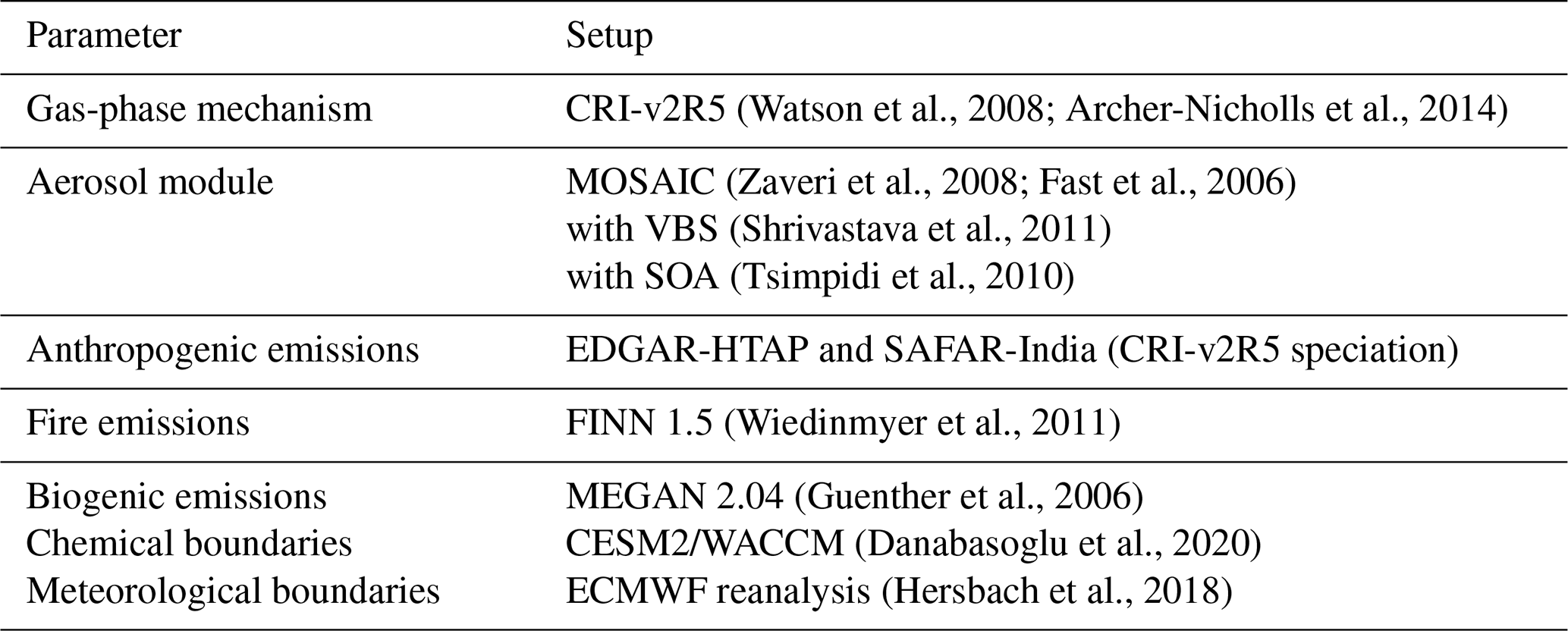
The Weather Research and Forecasting model coupled with Chemistry (WRF-Chem) is used to simulate the emission, transport, mixing and chemical transformation of trace gases and aerosols concurrently with meteorological data (Grell et al., 2005; Fast et al., 2006). Here, WRF-Chem version 3.8.1 is run with a 15 km domain, 127 × 127 grid cells (Fig. 1) and a simulation period from 19 April–29 May 2018, with substantial modification – for more details, see below. This period was selected in order to compare with aerosol measurements performed at New Delhi (Reyes-Villegas et al., 2021). Table 1 lists the components that contribute to our model setup, including the chemistry and aerosol schemes, emission inventories and boundary condition specifications. Gas-phase chemistry is simulated with the Common Representative Intermediates (CRI) mechanism, which permits a reasonably detailed representation of volatile organic compound oxidation. The aerosol chemistry is simulated using the sectional MOSAIC module (Zaveri et al., 2008), including N₂O₅ heterogeneous chemical reactions (Archer-Nicholls et al., 2014; Bertram and Thornton, 2009), and is coupled to the aqueous phase, which allows aerosols to act as cloud condensation nuclei, as well as to the removal of aerosols through wet deposition processes. The aerosol size distribution in MOSAIC is described by eight size bins spanning a dry particle diameter range of 39 nm to 10 µm (Zaveri et al., 2008).

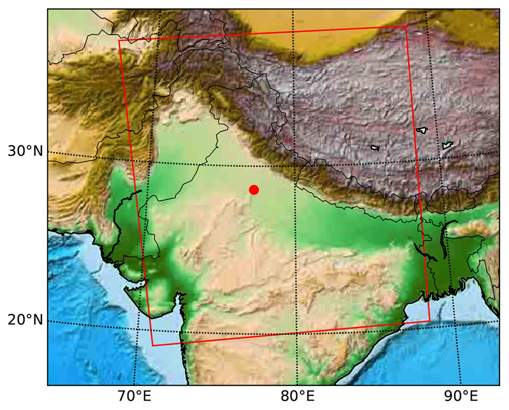
Figure 1 WRF-Chem model domain with topography data. The red marker highlights the location of IMD New Delhi, where the AMS observations were taken, and the red rectangle shows the area that covers the model results.

Table 1 WRF-Chem setup.

Our main modifications are focused on the treatment of the organic aerosol (OA) components. Primary organic aerosol (POA) is treated as semi-volatile, using the volatility basis set (VBS) treatment of Shrivastava et al. (2011). Their nine-volatility-bins VBS scheme has been adapted for use in the eight-size-bins version of MOSAIC. Secondary organic aerosol (SOA) has been included based on the scheme described in Tsimpidi et al. (2010), providing anthropogenic (ARO1 and ARO2 in the original scheme, SAPRC99) and “biogenic” (isoprene and monoterpenes) SOA components, each covering four volatility bins with C^* values (at 298 K) of 1, 10, 100 and 1000 µg m⁻³. ARO1 represents the aromatics with hydroxide (OH) reaction rates less than 2 × 10⁴ ppm⁻¹ min⁻¹, and ARO2 represents the aromatics with OH reaction rates greater than 2 × 10⁴ ppm⁻¹ min⁻¹. In mapping these to the CRI-v2R5 scheme, we have used toluene and benzene as the precursors for the ARO1 reactions, oxyl (xylene and other aromatics) for the ARO2 reactions, and a pinene for the monoterpenes. Indicative SOA yields are given in Table S1 in the Supplement. Co-condensation of water has been added for these semi-volatile organics, and they have been coupled to the aqueous phase in the same manner as other aerosol compounds in MOSAIC. Previous studies have demonstrated that the condensation of semi-volatile organic material onto aerosol particles substantially increases the soluble mass of particles, their chemical composition and eventually their effective dry size (Topping et al., 2013; Crooks et al., 2018). The mapping of CESM2 (Community Earth System Model 2) and WACCM (Whole Atmosphere Community Climate Model, version 5) compounds to CRI-v2R5 (Common Representative Intermediates) and MOSAIC components for the chemical boundaries is detailed in Table S2 in the Supplement. A spin-up period of 11 d (from 19 April to 1 May) was used. The meteorological driving fields were taken from ERA5 reanalysis data. Spectral nudging of the UV wind parameters, temperature and geopotential height variables to those above model level 18 and for wavelengths greater than 950 km was used. The domain is made up of 38 model layers, variable height and terrain following model levels up to a pressure of 50 hPa. The first model layer has a mean height of 59 m over Delhi (and a mean height of 56 m over the whole model domain).

Previous studies using the VBS have used scaling factors from POA to derive SVOC emissions in each volatility bin based on equilibrium-partitioning calculations, as well as volatility distributions based on laboratory studies and assumed oxygenation and chemical reaction rates (Shrivastava et al., 2011; Fountoukis et al., 2014). To investigate the impact of these assumptions on the model predictions, we have modified the model code so that the VBS emissions, the oxygenation rates and VBS reaction rates can be directly controlled via namelist options. The parameters which are perturbed in this way for this study are described in more detail in Sect. 2.3.

The volatility distribution of open biomass burning emissions is taken from May et al. (2013) and multiplied by a scaling factor of 3 (based on equilibrium-partitioning calculations) to ensure a reasonably similar condensed mass at emission as that reported in the Fire INventory from NCAR (FINN) 1.5 emission dataset. Similar calculations have been made in previous studies, giving roughly the same scaling factor (Shrivastava et al., 2011; Fountoukis et al., 2014; Denier van der Gon et al., 2015; Ciarelli et al., 2017). Before applying the scaling factor, we assumed a ratio of matter mass to carbon mass of 1.4, dividing the emission inventory matter mass by this to obtain the carbon mass. Within the model, each VBS compound is stored as two variables, the oxygen part and the non-oxygen part. When adding the emissions, we multiply the carbon mass by 1.17 to get the non-oxygen mass (carbon plus other atoms) and by 0.08 to get the oxygen mass. These scaling factors were taken from Shrivastava et al. (2011). We then apply the SVOC scaling factor and volatility distribution to give the final SVOC emission profile. The IVOC scaling factor is applied to the same base emissions to get the IVOC emission profile. The volatility distribution for anthropogenic emissions is also multiplied by a scaling factor of 3 for the same reasons as above. It is worth mentioning that the perturbed space explored here is embedded in the parent VBS scheme that has been adopted. There have been a large number of developments in and variants of the VBS aiming to address particular questions related to SOA formation at various levels of complexity, for example the mechanistic measurement-constrained radical 2D-VBS, which examines the role of extremely low-volatility organic compounds (ELVOCs) and ultra-low-volatility organic compounds (ULVOCs) in new-particle formation (Zhao et al., 2020, 2021). In the current study, our implementation has been developed from the VBS version available in the distribution version of WRF-Chem, and our results should be interpreted in the context of the structural capabilities and limitations therein. More information about the VBS distributions and parameter space setup is in Section S1 in the Supplement.

Anthropogenic emissions are derived from the EDGAR-HTAP, SAFAR-India (CRI-v2R5 speciation) and NMVOC global emission datasets, with NMVOC emissions speciated for the CRI-v2R5 chemical scheme, and diurnal activity cycles are applied to the emissions based on emission sectors in Europe (Olivier et al., 2003). We used these diurnal activity cycles (Fig. S1 in the Supplement), as there were no data available for activity behavior in Delhi. Biogenic emissions are calculated online using the MEGAN model (Guenther et al., 2006). Biomass burning emissions are taken from the FINNv1.5 global inventory (Wiedinmyer et al., 2011).

2.2 Observations

Aerosol observations were made at the Indian Meteorology Department (IMD) at Lodhi Road in New Delhi, India (lat 28.588, long 77.217), from 26 April to 30 May 2018 as part of the PROMOTE campaign (Reyes-Villegas et al., 2021). A high-resolution time-of-flight aerosol mass spectrometer (HR-TOF-AMS, Aerodyne Research Inc.), hereafter referred to as AMS, was used to measure mass spectra of non-refractory particulate matter with an aerodynamic diameter equal to or lower than 1 µm (PM₁), including organic aerosols (OAs), sulfate (SO${}_{\mathrm{4}}^{\mathrm{2}-}$), nitrate (NO${}_{\mathrm{3}}^{-}$), ammonium (NH${}_{\mathrm{4}}^{+}$) and chloride (Cl⁻), in a 5 min time resolution. The AMS operation principle has been previously described by DeCarlo et al. (2006). The AMS was calibrated during the campaign for the ionization efficiency (IE) of nitrate and the relative ionization efficiency (RIE) of other inorganic compounds using nebulized ammonium nitrate and ammonium sulfate with a diameter of 300 nm. The data were analyzed using the IGOR Pro (WaveMetrics Inc., Portland, OR, USA)-based software SQUIRREL (SeQUential Igor data RetRiEval) v.1.63I and PIKA (Peak Integration by Key Analysis) v.1.23I. The organic-to-carbon (O:C) ratios were calculated with PIKA using the Improved-Ambient elemental analysis method for AMS spectra measured in the air (Canagaratna et al., 2015). The AMS data, OA mass concentrations and O:C ratios are used to compare with the following WRF-Chem model outputs: total organic matter mass concentration (Total_OM) and organic-to-carbon ratios (OC_ratio).

There were no planetary boundary layer height (PBLH) measurements available at IMD Lodhi Road; hence, PBLH data were sourced from ECMWF ERA5 with 0.25^∘ results at a 1 h resolution for the coordinates closest to the IMD site. Meteorology data were downloaded from https://ncdc.noaa.gov/ (last access: 5 January 2019) for the Indira Gandhi International Airport, India, meteorology station.

The meteorology data were used to interpret the diurnal behavior of the chemical species and to compare with meteorology outputs from WRF-Chem. A dataset of meteorology was not available at IMD. The use of meteorology from airports has been previously used and is considered to be representative of regional meteorology without being affected by surrounding buildings (Reyes-Villegas et al., 2016).

2.3 Perturbed parameter ensemble

To evaluate the sensitivity to variations in the VBS emission and processing parameters of our WRF-Chem model of the simulated OA over the New Delhi region, we generated a perturbed parameter ensemble (PPE). We choose a set of simulations with optimal space-filling properties that provide effective coverage across the multi-dimensional space of the uncertain model parameters. Here, we perturb 10 parameters of the WRF-Chem model that relate to semi-volatile POA emissions and the aging of these VBS compounds. The parameters correspond to five processes in the model, which are perturbed with respect to both anthropogenic emissions and biomass burning emissions. These process parameters are as follows:

1. VBS aging rate. This refers to the reaction rates of VBS compounds with OH – each reaction reduces the volatility of the compound by a factor of 10 (1 decade in saturation concentration, Ci^* and position) and adds between 7.5 % and 40 % oxygen (determined by the SVOC oxidation rate parameter, as below). Ci^* is the condensed mass loading at which half of the organic material in that volatility bin will be in the condensed phase and half will be in gas phase (Donahue et al., 2006).

2. SVOC volatility distribution. This parameter is expressed in terms of an equivalent age, determined using a simple aging model. At time = 0, all VBS molecules will be highly volatile, with a Ci^* = 4. These compounds are processed at a fixed reaction rate (at each step, 0.1 % of the gaseous mass in a volatility bin is moved to the next volatility bin), with simple equilibrium partitioning of the VBS components between the gas and condensed phases (to roughly simulate the manner in which VBS compounds are partitioned and aged within the WRF-Chem scheme). This processing reduces the overall volatility of the VBS compounds, first providing a spread of mass across the volatility range before accumulating the mass in the lowest-volatility bins until 90 % of the VBS mass is in the Ci^* = −2 volatility bin (time = 1). This parameter is a scalar variable (between 0–1) that indicates the dimensionless position between these two points and has an associated volatility distribution. After examining the range of volatility distributions given by this simple aging model, we have chosen to use distributions within the range of 0.05 to 0.4. Using values above 0.05 ensures that there will always be some lower-volatility compounds to condense. Above 0.4, almost everything is condensed, so we have excluded values above this so that our PPE does not become too heavily weighted towards these scenarios. The scalar variable represents a sensible range of possible emitted-volatility distributions. A method was needed by which we could represent the variation of possible volatility distributions within the process emulator. The direct approach would be to include a scaling factor for each volatility bin as separate parameters. However, this would have greatly increased the complexity and size of our parameter space, and these parameters would not be independent of each other, leading to a lot of wasted parameter space, waste in the use of our limited computer resources available for the PPE simulations and the assumptions for our variance-based sensitivity analysis becoming invalid. Instead, we used a simple reaction model, where each step in a fraction of each volatility bin would be aged and moved to the next volatility bin. This approach also allowed us to include some simple partitioning, with aging process stopped for any condensed matter, replicating the behavior of the model these distributions will later be injected into. Given that we used a simple, fractional aging process, it would not be appropriate for us to try to relate it to a physical variable. We have included Fig. S2 instead, which gives an example volatility distributions through the range of this scalar value used in our study.

3. SVOC oxidation rate. This parameter represents the degree of oxidation that occurs with (or is induced by) each reaction with an OH molecule. Previous studies have used values between 0.075 (7.5 %) extra oxygen (or one oxygen atom; Robinson et al., 2007) and 0.40 (40 %) extra oxygen (or five extra oxygen atoms per reaction; Grieshop et al., 2009). Grieshop et al. (2009) stated that, with 7.5 %, there is not enough addition of oxygen to the organic mass, while with the 40 %, there is a noticeable improvement to the OA oxygen content with little effect on the predicted organic mass production. In our study, the lowest level is 0.075 extra oxygen (or one oxygen atom), and the uppermost level is 0.45 (or six extra oxygen atoms per reaction).

4. IVOC scaling. IVOC compounds bridge the gap from SVOCs to VOCs (log 10(C^*) 4–6). Including the IVOCs independently to parameter (2) (based on our simple aging model) enables us to still include these within the volatility distribution (this does restrict the impact of parameter (2) in terms of influencing the shape of the volatility distribution for the lower C^* values only). These IVOC emissions are calculated using a fixed volatility distribution, which scales from the non-volatile OA mass in the emissions inventory. The fractional emitted masses are as follows: 0.2 for Ci^* = 4, 0.5 for Ci^* = 5 and 0.8 for Ci^* = 6 (as shown in Fig. S2; $\mathrm{0.2}+\mathrm{0.5}+\mathrm{0.8}=\mathrm{1.5}$); this is the initial emission amount that then will be scaled by another factor, between 0–3, to probe the sensitivity of the model to the abundance of IVOCs.

5. SVOC scaling. This parameter is the scaling factor of the SVOC emissions, which have been given a volatility distribution by parameter 2. Traditionally, such scaling has been used to ensure that the condensed mass of the emitted SVOC is the same as the non-volatile OA mass in the emissions inventory; however, this scaling could also be used to off-set errors in the emission inventory estimates of OA emissions. The scaling needed to ensure that the emitted condensed mass is the same will never be less than 1 but could go to ×20 (or more) for the younger SVOC volatility ranges (as estimated using the equilibrium-partitioning tool for parameter 2). However, in order to accommodate potential overestimates of the emission inventories and to avoid too much OA being generated after aging of any highly volatile emissions, we chose an SVOC scaling range of 0.5 to 4.

Table 2 shows the uncertainty ranges applied to each of the parameters that we explore with the PPE, and Table S3 in the Supplement shows an example of a “namelist.input” file with the parameters to control the VBS scheme that was used to create the model simulation. A total of 111 model simulations make up the ensemble. Following the statistical methodology outlined in Lee et al. (2011), the combinations of input parameters used for the simulations in the PPE were selected using an optimal Latin hypercube statistical design algorithm (Stocki, 2005), providing good coverage of the multi-dimensional parameter space. The selection of combinations was performed in three subsets for use in building statistical emulators to densely sample key outputs from the model over its uncertainties. First, a single design of 61 runs was generated for training the emulators (subset 1), and then a second set of 20 runs was made that augmented the emulators into the larger gaps of the first design, for use in validating the emulators (subset 2). On an initial comparison to observations, the observations were found to be outside the range of the PPE's output, and following an investigation into this, the lower bound of the anthropogenic SVOC scaling parameter (parameter 5) was extended from 0.5× down to 0.1×. Hence, an extra (third) set of 30 runs was designed and simulated to cover the extended parameter space (subset 3), leading to a total of 111 runs in the final PPE. The configuration files for each model run are given in the Lowe et al.  (2023b) dataset (https://doi.org/10.5281/zenodo.7904011), and Table S4 in the Supplement provides a list of model runs that make up the PPE with their respective values.

Table 2 Range of the parameter space used for SVOCs co-emitted within anthropogenic POAs in the PPE with 111 model variants.

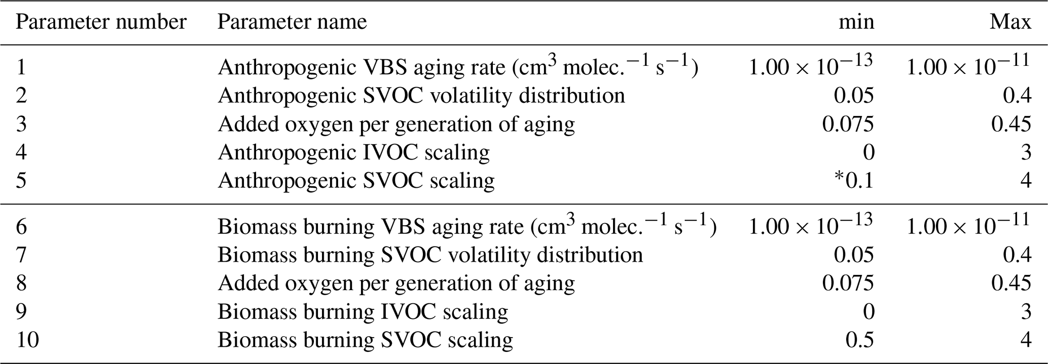
^* A total of 81 runs were performed with an anthropogenic SVOC scaling min  = 0.5 and max  = 4, and 30 runs were performed with an anthropogenic SVOC scaling min = 0.1 and max = 0.5. This due to a min = 0.5 and max = 4 giving high organic mass concentrations when compared with AMS.

2.4 Emulation

For each PPE member, a time series of the OC_ratio and Total_OM from the WRF-Chem model run was extracted at the closest coordinates to the IMD site (lat 28.628, long 77.209) in the model output. Gaussian process emulators (O'Hagan, 2006; Lee et al., 2011) were built using the PPE. Similarly to the approach described in Johnson et al. (2018), initial emulators were constructed using only training simulations (subsets 1 and 3), and these were validated using the validation runs (subset 2). Once validated, a further new emulator was then constructed using both the training and validation simulations of the PPE together as training data to obtain a final emulator based on all of the information that the PPE contains. An additional verification of the quality of each final emulator was obtained via a leave-one-out validation procedure (where each simulation in turn is removed from the full set of 111 runs, and a new emulator is built and used to predict that removed simulation).

Monte Carlo sampling of the emulators enabled dense samples of model output to be generated over the 10-dimensional parameter uncertainty of the model. We produced output samples for a set of 0.5 million input parameter combinations across the uncertainty space, hereafter called model variants, to explore the model's uncertainty.

2.5 Model evaluation

Alongside the emulation, outputs from the 111 model runs (OC_ratio and Total_OM) were additionally evaluated against the AMS observations (O:C and OA) using various model evaluation tools, including the fraction of predictions within a factor of 2 (FAC2), mean bias (MB) and the index of agreement (IOA). Section S3 of the Supplement provides a detailed explanation of the calculations for each evaluation metric and information on how to interpret the values.

3 Results and discussion

3.1 Model outputs and observational analysis

The model outputs of the central WRF-Chem run from the original parameter space (subsets 1 and 2) are used to compare with observations in order to analyze the model performance. As mentioned in the methods section, the VBS setup will directly affect OA concentrations and PM. The oxidative budget for inorganic chemistry is not directly affected; however, by changing the aerosol size distribution, there are some indirect effects on inorganic aerosol and gaseous species through changes in aerosol water content, cloud fields and aerosol–radiation interactions. Figure 2 shows the comparison for the full dataset (1–29 May 2018) between model outputs and observations performed at IMD Lodhi Road, where we see higher PM_2.5 and NO_x concentrations in the model simulation. The high NOx concentrations in the model seem to be related to high NO₂ concentrations, as the NO concentrations are in line with the range of the observations of NO. Looking at the meteorological parameters, we can see similar temperatures and wind speeds between the model and observations, with lower RH and higher PBLH in the model.

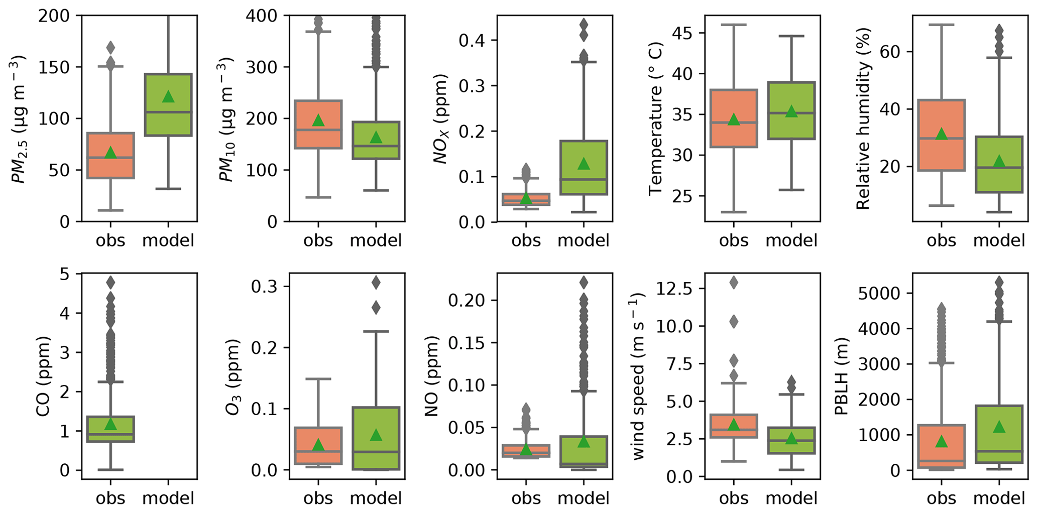
Figure 2 Comparison of observations (At Lodhi Road for air quality and at IGI Airport for meteorology parameters) and model outputs of various parameters. May 2018. Bars highlight medians, quartiles and 95 %; triangles highlight the mean.

3.2 Model runs and AMS observations

Here, we analyze and compare the mean values of Total_OM (modeled particle phase) and OC_ratio for the full period, 1–29 May 2018, of the 111 WRF-Chem model runs (Table S4 in the Supplement) with the AMS observations (OA and O:C). The top panel in Fig. 3 shows a bar plot of the mean OC_ratio for the model runs colored by the mean total_OM concentrations. The bottom panel shows the mean total_OM concentrations for the model runs colored by the mean OC_ratio. The model runs are sorted from low to high values of the y variable. The continuous and dashed red lines show the mean ± 1 standard deviation (SD) of the O:C ratio (top) and OA (bottom) measured with the AMS. In general, compared to mean values measured with the AMS, a large number of WRF-Chem runs had a low O:C_ratio and high mean Total_OM concentrations. The bottom panel shows the mean total_OM concentrations of 47 runs lying within 1 SD of the mean OA concentration of 21.77 µg m⁻³ measured with the AMS. Moreover, the model runs with mean Total_OM concentrations near the mean OA concentrations have OC_ratio mean values near the O:C mean AMS value (0.5), with a cyan color. We explored a range of emission multipliers (both IVOC and SVOC scaling). These upper limits, which have been of an appropriate magnitude for previous studies in other locations using different emission datasets (e.g., Shrivastava et al., 2011), turned out to be too high for our emission dataset, and these are the model runs which produced the very high OM mass loadings (rather than these being predominately caused by high oxidation rates). When the OM mass loading is high, more of the higher-volatility (and, here, less-aged) compounds condense into the condensed phase. The VBS scheme we have used has only gas-phase reactions, and so once in the condensed phase, these compounds do not age further. This process leads to the lower mean O:C ratios that are observed here. This analysis shows a number of model runs with mean Total_OM and OC_ratio values near the mean values measured with an AMS.

Figure 3 Analysis of the 111 model runs for the full period. Mean OC_ratio colored by mean Total_OM (top plot) and mean Total_OM colored by mean OC_ratio (bottom plot). The red lines highlight the mean ± SD of AMS observations (O:C top and OA bottom). The mean AMS values are O:C = 0.5 and OA = 21.77 µg m⁻³.

3.3 Diurnal analysis of WRF-Chem runs

The high-time-resolution data collected with the AMS provide the opportunity to analyze the WRF-Chem outputs in more detail, for example by looking at the diurnal cycles. Figure 4 shows the diurnal cycles of chosen WRF-Chem runs with Total_OM concentrations and OC_ratio close to the AMS observations. In the model runs, we were able to span high and low Total_OM and OC_ratio. However, in the case of OC_ratio, we were not able to span the range of the O:C from AMS observations with mean values of 0.3 at night and 0.7 during the day. Looking at the Total_OM concentrations, we identified two potential structural errors in the WRF-Chem outputs, namely the early-morning peak and the late-evening low concentrations. This could be due to application of unsuitable diurnal activity cycles to the emissions or WRF-Chem not being able to capture completely the dynamics of the planetary boundary layer. With no activity data available for Delhi, we used diurnal cycles of activities based on emission sectors in Europe (Olivier et al., 2003; Fig. S1 in the Supplement). We can observe in Fig. S5 in the Supplement a slightly better comparison in terms of the CO model vs. observations, with flatter CO concentrations when looking at the observations. For the diurnal cycles of meteorology (Fig. S4), we can see that the model agrees with the PBLH-ERA5 in the early morning and until 14:00 h, the time when PBLH-ERA5 starts dropping and PBLH-Model remains high, perhaps preventing concentrations from accumulating. This makes building and testing the emulator challenging, as we may get the correct concentrations for the wrong reasons. The emulator can be built over a specific time period and can be compared with the observations. Hence, the emulator was built over the following two periods of interest: the full period (1–29 May) and a period where no potential structural errors were identified from 14:00–16:00 h for 1–29 May (2–4 p.m. period). Emulator analysis involving the filtering of model results to avoid structural errors has been successfully performed previously in constraining a climate model (Johnson et al., 2020). Looking at the mean OC_ratio and Total_OM of the model runs for the 2–4 p.m. period (Fig. S6), 34 runs lay within 1 SD of the OA mean concentration (12.20 µg m⁻³) measured with the AMS compared to the 47 runs identified from Fig. 3. This means that, even by analyzing the 2–4 p.m. period, we still have model runs that cover the AMS observations.

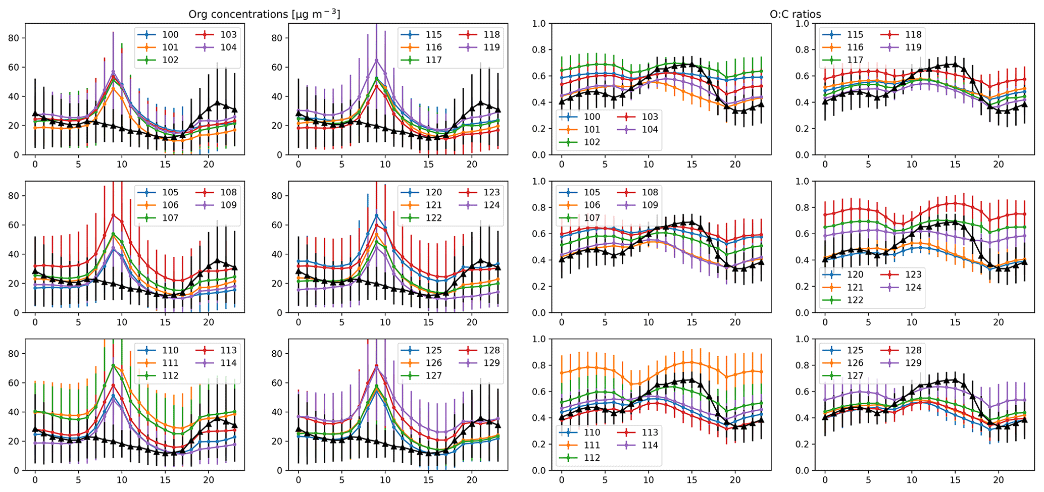
Figure 4 Diurnal cycle of selected WRF-Chem runs with values near the AMS observations (black line).

3.4 Model evaluation

There are various tools that can be used to compare the model outputs with the observations. In this study, we use a number of statistical metrics (see Sect. S3 in the Supplement for a detailed description of each metric we consider) to evaluate the ensemble of 111 model runs for the 2–4 p.m. period and the full period. The fraction of predictions within a factor of 2 (FAC2) represents the fraction of data where predictions are within a factor of 2 of observations. The mean bias (MB) gives an indication of the mean over- or underestimation of predictions. The Index Of Agreement (IOA) is a commonly used metric in model evaluation (Willmott et al., 2012), ranging between −1 and +1, with values close to +1 representing a better model performance. Table S3 in the Supplement shows the results of the model evaluation for the 2–4 p.m. period, and Table S4 in the Supplement shows the results for the full period. When comparing the performance of the two periods, the model runs of the 2–4 p.m. period demonstrate a better performance, with 103 runs for O:C and 29 runs for OA with FAC2 >0.6 compared to 94 runs for O:C and 4 runs for OA with FAC2 >0.6 for the full period. The negative MB in O:C suggests that the models underestimate the O:C ratios (between −0.01 to −0.15) measured with the AMS. However, the FAC2 values of 0.96 and higher indicate that the models do a good job overall at simulating the O:C ratios. This is not the same for OA concentrations, where the models show an overestimate of the concentration compared to observations and where only 0.56–0.62 of predictions were within a factor of 2 of the OA observations.

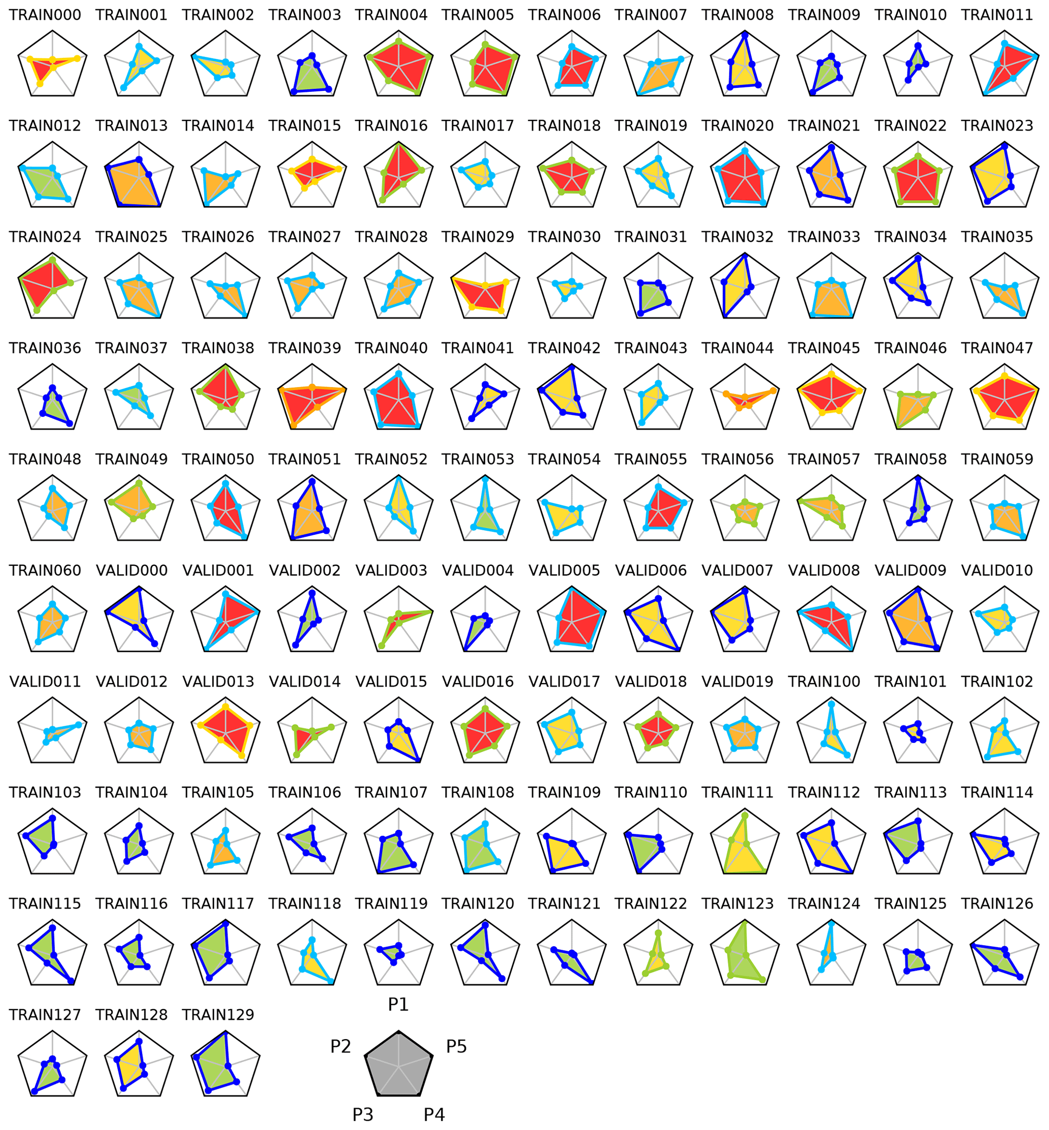
Figure 5 Relative variation (%) of the five anthropogenic PPEs (1–5) for the 2–4 p.m. period. Each pentagon represents the 5-D parameter space, and the positions of the dots connected with lines show the position of each parameter within its range for that specific ensemble member. The filled area within the dots represents the explored parameter space in each ensemble member. Counterclockwise from the top, there are the following five anthropogenic parameters: VBS aging rate (P1), SVOC volatility distribution (P2), SVOC oxidation rate (P3), IVOC scaling (P4) and SVOC scaling (P5). The values of the five parameters have been normalized dividing by their respective maximum values; hence, their values in this plot range from 0–1. The color in the lines and dots represents the FAC2 values from the O:C analysis, and the fill color represents the FAC2 values from the OA analysis. Red = 0–0.2, orange = 0.2–0.4, yellow = 0.4–0.6, green = 0.6–0.8, light blue or cyan = 0.8–0.9, and blue = 0.9–1.0.

Figure 6 Validation of the full (a and b) and 2–4 p.m. (c and d) periods for O:C ratio and total OM. Circles are the original 81 runs. Squares with error bars in blue are the new 30 runs with low settings of the anthropogenic SVOC scaling parameter (which has led to low aerosol mass). Runs where the actual model output lies outside the 95 % prediction interval of the emulator are shown in red.

The IOA provides similar results with a better model performance in the 2–4 p.m. period, with 10 model runs for the 2–4 p.m. period and only 2 runs for the full period with IOA values equal to or higher than 0.45. It is interesting to see that, while FAC2 was higher for OA and O:C in the 2–4 p.m. period runs compared to in the full period, IOA values in 2–4 period were high with OA but low with O:C, which reached IOA values of 0.53 in the 2–4 p.m. period and 0.56 in the full period. Previous studies performing modeling evaluation determined similar IOA values using various models (Ciarelli et al., 2017; Fanourgakis et al., 2019). For instance, Chen et al. (2021), modeling SOA formation, obtained IOA values between 0.39–0.49. Huang et al. (2021) published recommendations on model evaluation and identified IOA values of around 0.5 for organic carbon. Lee et al. (2020) performed a sensitivity analysis for two different SOA modules and obtained IOA values of 0.46–0.52.

The model evaluation metrics, along with the parameter setup for each ensemble member, allow us to analyze the model setup that gives a better performance. Figure 5 shows the relative variation (%) of the five anthropogenic parameters of the PPE (1–5) for the 2–4 p.m. period (Fig. S7 in the Supplement shows the analysis for the full period). Each pentagon represents the 5-D parameter space, and the positions of the dots connected with lines show the position of each parameter within its range for that specific ensemble member. The filled area within the dots represents the explored parameter space in each ensemble member. We analyze the five anthropogenic PPEs only, since the five parameters related to biomass burning represented a low contribution to the Total_OM concentrations. We are looking for blue, light-blue or green colors in the lines and dots (high FAC2 values from the O:C analysis) and blue, light-blue or green colors in the filled area (high FAC2 values from the OA analysis) to identify the model runs with a good evaluation. In Fig. 5, we can see that the best runs according to the O:C and OA model evaluation are TRAIN127 and TRAIN121, with other TRAIN runs also demonstrating good performance, such as runs 126, 036, 117, 104, 115, 119 and 058. In general, these model runs have low SVOC volatility distribution (emitted VBS compounds are more volatile) and SVOC scaling. TRAIN127 and TRAIN121 have low VBS aging rate, SVOC volatility distribution and SVOC scaling, with either a high SVOC oxidation rate or high IVOC scaling.

3.5 Emulator analysis

3.5.1 Emulator building and testing

Once we confirm that the ensemble of 111 model runs spans the AMS observations, we can use it to build the emulator. The emulators are tested using the leave-one-out validation approach (Johnson et al., 2018). In this analysis, each ensemble run is first excluded from the emulator build, and then the emulator is used to predict the output at the parameter setting of the excluded run. Figure 6 shows plots of the emulator predictions (with 95 % credible intervals from the emulator model) vs. the model outputs of the 111 runs from the leave-one-out validation for OA. Predictions from a perfect emulator would follow exactly along the 1:1 line on the plots.

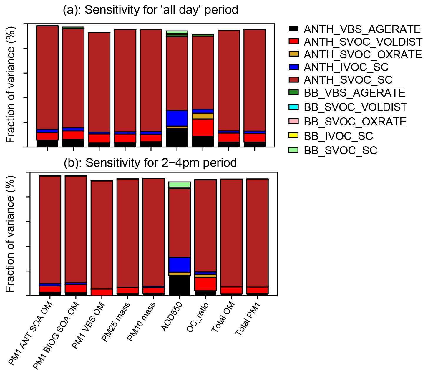
Figure 7 Sensitivity evaluation of the 10 chosen parameters for the 2–4 p.m. period (a) and for the full period (b).

Figure 8 A total of 0.5 million emulator samples, before constraint, covering the full parameter uncertainty space of the model for the full period (a and b) and for the 2–4 p.m. period (c and d). Red highlights the AMS mean ±SD observations.

We built and tested the emulator for the full period (1–29 May) to have an overview of the emulator performance. The emulator can be built over a specific time period to compare with the observations. This allows one to study the model performance under different conditions, i.e., high or low aerosol concentrations, day or night, etc. We selected four period time slots to build and test the emulator under high and low Total_OM concentrations and two time slots. These four emulators showed a good validation analysis (Refer to Sect. S5.1.1 in the Supplement). However, due to the potential structural errors identified from the diurnal analysis (Sect. 3.3), we will focus on the selected period without structural errors, the 2–4 p.m. period. Figures S11 and S12 in the Supplement show the spread of Total_OM and OC_ratio, respectively, for the ensemble of 111 model runs vs. the 10 parameters.

We see in Fig. 6 that, overall, the emulators built for the two periods (full period (Fig. 6a and b) and 2–4 p.m. period (Fig. 6c and d)) show a good performance. For the 2–4 p.m. period, in terms of Total_OM, we see only nine runs that are not within the 95 % CI from prediction (red markers), and in terms of OC_ratio, we see 10 runs that are not within the 95 % CI from prediction. With the 30 new runs (error bars in blue), we managed to reduce the Total_OM concentrations with good prediction ability from the emulator. However, there is a compromise in the OC_ratio, with eight runs with high OC_ratio values that at not within the 95 % prediction interval of the emulator.

3.6 Emulator sensitivity analysis

We use a variance-based sensitivity analysis (Lee et al., 2011; Johnson et al., 2018) to decompose the overall variance in the model output for key variables of interest into percentage fractions for the 10 parameters. This analysis was performed to the full period and for the 2–4 p.m. period (Fig. 7). Looking at the parameters for the two periods, the anthropogenic SVOC scaling has the highest contribution to the variance, which suggests that constraining this parameter would lead to a reduction in the uncertainty in these outputs from the model. Anthropogenic SVOC volatility distribution has some impact on O:C ratios with a fraction of variance of around 15 %.

3.6.1 Impact of constraint on uncertainty

The emulator was used to predict model outputs for a sample of size 0.5 million for the full period and for the 2–4 p.m. period. Figure 8 shows the probability distribution of OC_ratio and Total_OM predicted over the full parameter uncertainty. The AMS means ± 1SD are shown in red. We can see that the higher density (lower values) of the Total_OM shows a good agreement with the AMS-OA concentrations. However, in the case of O:C, the higher density lies on the low side of the O:C ratios compared to the O:C-AMS observations, which lie in the upper tail of the predicted distribution. The OC_ratio varies within the two periods, with a wider density range for the full period, 0.25–0.55, which represents the variability of the OC_ratio over the full day. In the case of the 2–4 p.m. period, we can see more-narrow density, 0.3–0.5, which, while lower than the mean O:C ratio measured with the AMS (0.65), may be representative of the O:C ratios estimated with the WRF-Chem runs. This suggests that, when analyzing diurnal behavior of WRF-Chem outputs without structural errors, we would be able to analyze in more detail the WRF-Chem performance over different hours of the day.

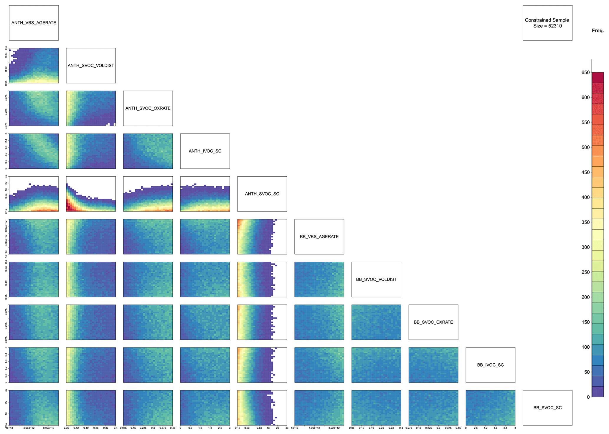
Figure 9 Two-dimensional histogram for joint constraint effect (Total_OM and OC_ratio) accounting for emulator uncertainty. Retains 52 310 variants from 0.5 million emulations (∼ 10.46 %).

Figure 10 Marginal parameter constraints: joint constraint effect (Total_OM and OC_ratio).

3.6.2 Constraint effect

The AMS observations, OA concentrations and O:C ratios are used to constrain the emulation, applying an observation uncertainty as mean ± SD. With the mean as the emulator prediction and a 1 SD uncertainty, we apply the constraint when accounting for emulator prediction uncertainty by retaining the variant if the range mean ± SD overlaps with the observation uncertainty range.

Figure 9 is a 2-D histogram for joint constraint (Total_OM and OC_ratio) for the 2–4 p.m. period, with color showing the frequency of variants in a pixel of an underlying grid arranged as a pairwise space (shown by the label box on each axis (above or to the right)). Each 2-D pairwise space has been split into a 25 × 25 uniform grid to calculate the frequencies. Where the plots show yellow to red, more variants are retained than in the green and blue areas, highlighting the most likely (higher-probability) area of space. This analysis shows that, when constraining both Total_OM and O:C ratios, the emulator retains 52 310 variants from 0.5 million, which is approximately 10.46 % of the original variants generated.

White areas indicate that no variants at all are retained in that pixel, so that 2-D space is ruled out with respect to all 10 dimensions. (probability = 0). Where the color is uniform, e.g., biomass burning parameter plots in Fig. 9, the parameter is essentially un-constrained, and all parts of parameter space with respect to those two parameters are equally likely and/or covered by variants (as it was before the constraint was applied). These plots show where in the parameter space is most likely given the comparison to observation. These are the variants that we cannot rule out (i.e., that are plausible) given the uncertainty – it does not mean they are all good. It is worth mentioning that, with this analysis, we do not locate the exact best run; instead, we provide a range of potential combinations to test the WRF-Chem setup.

These results agree with the analysis in the model evaluation (Sect. 3.4). Figure 9 shows, in red color, the higher probability that, with low SVOC volatility distribution and low SVOC scaling, would give a good model performance. However, there is no clear pattern with the other parameters.

3.6.3 Marginal parameter constraints

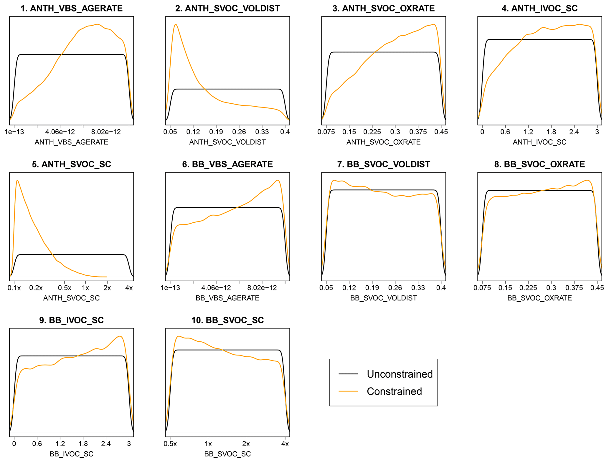
Figure 10 shows the marginal constraint (1-D projection) on the parameters over their ranges. The unconstrained sample (black) has even coverage (i.e., it is sampled uniformly) across all parameter ranges and the parameter space. The unconstrained sample covers the full 10-D space.

Where the probability density function (PDF) of the constrained sample is above the black unconstrained PDF, the likelihood of the parameter taking a value at that point of its range is increased in terms of constraint (more probability). Where it is below, it is now less likely in terms of constraint (less probability). The more squashed the unconstrained distribution is, the more the likelihood of the parameter taking values in the range with a higher density is. This analysis is a useful tool to identify the more likely values of the 10 parameters over all the parameter space. Here, we can see that low SVOC volatility distribution and low SVOC are clear parameter values that we can use to improve the WRF-Chem model setup. Other parameters that we can start testing on WRF-Chem are high biomass-burning (BB) VBS aging rate (6) and BB IVOC scaling (9). It is worth highlighting the similarity of the effects on the anthropogenic and biomass burning parameters.

3.7 Analysis of model evaluation and emulator runs

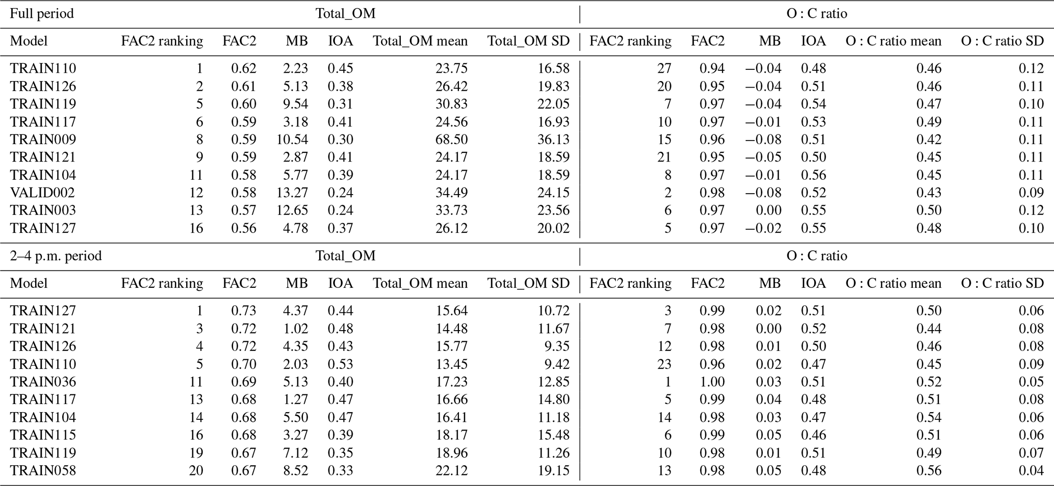
Table 3 shows the WRF-Chem runs with both mean organic and mean O:C values close to AMS observations for the two periods and also for the selected runs from the 2-D histograms (Fig. 9). Here, we can see a couple of interesting findings. First, the O:C ratios presented a better performance with the model evaluation metrics, specifically in terms of FAC2 values higher than 0.9 compared with FAC2 values up to 0.73 for the total OM. Looking at the total OM, there are higher FAC2 values in the 2–4 p.m. period, which might be related to the structural errors impacting the model performance in the full period. The MB provides an estimation of the overprediction of the Total_OM. In this study, WRF-Chem runs, in generally overpredicted the total OM concentrations. Hence, MB is an important metric. In both periods, there are runs where the overprediction was 5 µg m⁻³ or lower, i.e, TRAIN110, TRANI121, TRAIN117, etc. This highlights the use of all the analyses presented in this study where we are able to identify probable values for the VBS model parameters and where we are able to model total OM and O:C ratios.

Table 3 Analysis of model evaluation metrics and comparison with observations for the full and 2–4 p.m. periods. The FAC2 ranking is based on high FAC2 values of the Total_OM analysis. Mean AMS values for the full period are OA = 21.77 µg m⁻³ and O:C =  0.5. Mean AMS values for 2–4 p.m. period are OA = 12.20 µg m⁻³ and O:C = 0.67.

4 Conclusions

In this study, we aimed to determine an effective way of tuning the VBS scheme using observations and also to learn about the processes controlling OA in Delhi. The WRF-Chem model runs with the VBS setup that successfully spans the OA concentrations, and O:C ratios from AMS observations can be identified, with many model runs overestimating organic mass concentrations and underestimating the O:C ratios compared with AMS observations. However, we identified two structural errors in the model related to a combination of unsuitable diurnal activity cycles applied to the emissions and/or WRF-Chem not being able to capture completely the dynamics of the planetary boundary layer. It is worth mentioning that these structural errors might also be related to the representation of other organic aerosol processes not represented by the VBS approach. As mentioned early in the introduction, this study only considers semi-volatile POA processes without accounting for perturbations in SOA parameters and deposition processes. Recent studies, for example, have examined particle-phase and multiphase chemistry in aqueous aerosols and clouds (Shrivastava et al., 2022) and reactions of SOA precursors with other radicals like chlorine relevant to Indian conditions (Gunthe et al., 2021). Future studies could be focused on studying other parameters such as deposition processes and the perturbations in SOA parameters.

The structural errors prevented us from providing an optimized VBS approach in WRF-Chem. However, we were able to apply the emulator in the following two periods: the full period (1–29 May) and the 2–4 p.m. period (14:00–16:00, 1–29 May) to present a methodology to evaluate a model's performance using Gaussian emulators and metrics such as FAC2, IOA and MB. Optimization is a stage-by-stage process; future analysis would imply conducting an emulation study to address diurnal activity and PBL directly, perhaps using NOx or total PM.

The performance of the two emulators, the full period and the 2–4 p.m. period, was similar, with the two emulators demonstrating a good prediction of the model outputs and presenting a similar high variance of the anthropogenic SVOC scaling (parameter 5). The model performance would be highly improved if we were able to constrain the input values for parameter 5.

When looking at the emulator sensibility analysis, we identified that the parameter anthropogenic SVOC scaling has the highest contribution to the variance, with fractions higher than 70 %. This suggests that constraining this parameter would lead to a reduction in the uncertainty in these outputs from the model. Anthropogenic SVOC volatility distribution has little impact on the fraction of variance on O:C ratios, with a fraction of variance of around 15 %. None of the parameters show a clear enough variance to improve the model performance.

The model evaluation analysis based on FAC2, IOA and MB agreed with the emulator analysis in identifying that using low SVOC volatility distribution and low SVOC scaling would give improved model performance. Based on the MB analysis, for both the full and the 2–4 p.m. periods, there are runs where the total OM overprediction was 5 µg m⁻³ or lower, i.e, TRAIN110, TRANI121, TRAIN117, etc. This overprediction is considered to be low compared to the mean Total_OM concentrations of ∼ 20–30 µg m⁻³. Hence, we are able to identify probable values for the VBS model parameters and are able to model total OM and O:C ratios in the range of the AMS observations.

The combination of the emulator analysis and the model evaluation metrics (FAC2, IOA and mean bias) allowed us to identify the plausible parameter combinations for the analyzed periods. The more plausible combinations were found to be with a low SVOC volatility distribution and low SVOC scaling, which means a more volatile distribution. The methodology presented in this study is shown to be a useful approach to determine the model uncertainty and to determine the optimal parameterization for the WRF-Chem VBS setup. This information is valuable to increasing our understanding of secondary organic aerosol formation, which in turn will help to improve regional and global model simulations and emission inventories, as well as in making informed decisions towards the improvement of air quality in urban environments.