Aerosol first indirect effect of African smoke at the cloud base of marine cumulus clouds over Ascension Island, southern Atlantic Ocean

The interactions between aerosols and clouds are among the least understood climatic processes and were studied over Ascension Island. A ground-based UV polarization lidar was deployed on Ascension Island, which is located in the stratocumulus-to-cumulus transition zone of the southeastern Atlantic Ocean, to infer cloud droplet sizes and droplet number density near the cloud base of marine boundary layer cumulus clouds. The aerosol–cloud interaction (ACI) due to the presence of smoke from the African continent was determined during the monsoonal dry season. In September 2016, a cloud droplet number density ACI_N of 0.3 ± 0.21 and a cloud effective radius ACI_r of 0.18 ± 0.06 were found, due to the presence of smoke in and under the clouds. Smaller droplets near the cloud base makes them more susceptible to evaporation, and smoke in the marine boundary layer over the southeastern Atlantic Ocean will likely accelerate the stratocumulus-to-cumulus transition. The lidar retrievals were tested against more traditional radar–radiometer measurements and shown to be robust and at least as accurate as the lidar–radiometer measurements. The lidar estimates of the cloud effective radius are consistent with previous studies of cloud base droplet sizes. The lidar has the large advantage of retrieving both cloud and aerosol properties using a single instrument.

1 Introduction

The importance of low-level marine boundary layer (MBL) clouds for the earth's radiative energy has long been recognized. Their high albedo (30 %–40 %) over a dark ocean reduces the flux of solar radiation into the ocean, while they contribute only slightly to the downward thermal radiation, due to their low altitude (and thus high temperature) inside the MBL (Albrecht et al., 1988). An estimated 4 % increase in MBL cloud cover could offset the warming due to a doubling of CO₂ (Randall et al., 1984). Aerosols are expected to modulate the low-level cloud cover through an aerosol-induced reduction in precipitation (Albrecht, 1989; Ackerman et al., 2000) or change the cloud short-wave albedo through an increase in cloud condensation nuclei (CCN) (Twomey, 1974, 1977). The increase in CCN could lead to an increase in cloud droplet number density and a decrease in cloud droplet size, provided that the moisture content is constant. This effect is known as the first aerosol indirect effect. Additionally, the absorption of short-wave radiation by aerosols will locally heat the atmosphere and may modulate cloud properties by enhancing evaporation (e.g. Wang et al., 2003; Xue and Feingold, 2006) or changes in thermodynamic stability.

In the subtropics, extensive stratocumulus cloud decks form over the pool of cold water created by upwelling ocean currents west of the continents. The descending branch of the Hadley circulation in the subtropics creates a strong temperature inversion at the top of the MBL, which the stratocumulus decks are generally unable to penetrate. The stratocumulus decks are maintained by radiative cooling at the top of the MBL. This creates a moist, well-mixed layer over a cold ocean surface. Trade winds transport this system northwest along a gradient in sea surface temperature towards the warmer Equator, and a transition to cumulus clouds is observed, driven by increased convection from the warmer underlying surface. When the cumulus clouds penetrate the inversion and entrain warm, dry air from the free troposphere, the stratocumulus cloud deck breaks up and gradually dissipates (e.g. Paluch and Lenschow, 1991; Bretherton and Wyant, 1997; Wyant et al., 1997). This generally accepted thermodynamic theory of stratocumulus-to-cumulus transition (SCT) observed in the subtropical oceans is complicated when precipitation (Yamaguchi et al., 2017) or the presence of aerosols are taken into account (Wang et al., 2003).

Aerosols have several reported competing effects on the SCT duration, depending on the vertical and horizontal distribution of the aerosols, age and composition of the aerosols, etc. Over Africa, smoke is injected into the atmosphere during the dry season of the monsoon, which is July–October in southern Africa (e.g. de Graaf et al., 2010; Zuidema et al., 2018). The vertical distribution of the smoke changes through the season, from a mean altitude in the MBL in July to the free troposphere in October, leading to an amplified low-cloud seasonal cycle (Zhang and Zuidema, 2021). The smoke is transported over the southeastern Atlantic Ocean (SEAO) in the free troposphere under influence of the anticyclic circulation over Africa (Garstang et al., 1996; Swap et al., 1996) and the southern African easterly jet (Adebiyi and Zuidema, 2016). Close to the continent, the smoke in the free troposphere is found well above the temperature inversion, separated from the cloud top, while further out over the ocean it is more often mixed with the cloud top after several days of transport following the subsiding large-scale circulation. Therefore, near the continent, the smoke in the free troposphere was found to delay the SCT by strengthening the temperature inversion at the top of the MBL during the day when smoke absorbs solar radiation and heats the atmosphere locally. The stronger inversion results in thicker stratocumulus clouds (Johnson et al., 2004; Yamaguchi et al., 2015). Further from the continent, smoke was found entrained in the cloud layer (Painemal et al., 2014; Rajapakshe et al., 2017), changing the cloud droplet number density (Diamond et al., 2018) and decreasing the low-level cloud cover (Ajoku et al., 2021), due to a weakening of the temperature inversion and evaporation of smaller cloud droplets (Johnson et al., 2004; Xue and Feingold, 2006; Zhou et al., 2017). The radiative heating by the smoke in the free troposphere influences the large-scale circulation itself by reducing the subsidence, leading to lower temperatures and increased moistening at the plume top (Diamond et al., 2022).

For precipitating clouds the effects are much more complicated (e.g. Zhou et al., 2017), and therefore precipitating clouds are not considered here.

Inside the MBL aerosols are typically mixtures of sea salt and smoke from the African continent during the biomass burning season. The composition of the aerosol mixtures changes during its residence inside the MBL, due to processing inside clouds, interaction with air and absorption of sunlight (Dang et al., 2022). The short-wave radiation absorption by smoke during the day changes the diurnal thermodynamics of the MBL (Zhang and Zuidema, 2019).

In this paper, a method is explored to study aerosol–cloud interactions of smoke around the base of the clouds around Ascension Island. Here, we focus on the base of a low-level broken cloud deck in the SEAO following the metrics specified in McComiskey et al. (2009) for changes in the cloud droplet effective radius R_eff and cloud droplet number density, as a function of changes in aerosol optical thickness τ_aer or aerosol extinction, as derived using one specific instrument, a UV polarization lidar.

Such an instrument was located on Ascension Island during a month in 2016 and a month in 2017 during the dry season in Africa. The UV lidar was part of the measurement campaign CLARIFY-2017 (Clouds and Aerosol Radiative Impacts and Forcing; Haywood et al., 2021), partnering with several ground-based and aircraft campaigns described in Sect. 2. The measurements in 2017 were affected by alignment problems, which resulted in a lower signal-to-noise ratio (SNR) compared to the 2016 measurements. Therefore, the measurements from 2016 are used mainly to show the aerosol–cloud interactions (Sect. 3.1). The consistency of the lidar measurements was investigated through comparison with the abundant additional campaign measurements both in 2016 and 2017, as described in Sect. 4.

Both aerosol properties from the aerosol layers and cloud properties from the cloud deck were derived from the lidar data, using a technique to infer cloud parameters based on polarization change due to multiple scattering near the cloud base (Donovan et al., 2015). In this set-up, only one instrument is needed to study the impact of aerosols on cloud albedo by relating the aerosol number density to the cloud droplet number density (Sarna and Russchenberg, 2016). The details of the retrievals of the aerosol and cloud properties are described in Appendix A. The lidar beam will not penetrate deep into the cloud layer due to the large scattering cross section of the cloud droplets in the UV. Therefore, the cloud measurement results are valid near the cloud base. In this study we relate the cloud properties to an altitude of 100 m above the cloud base height (see Sect. A4).

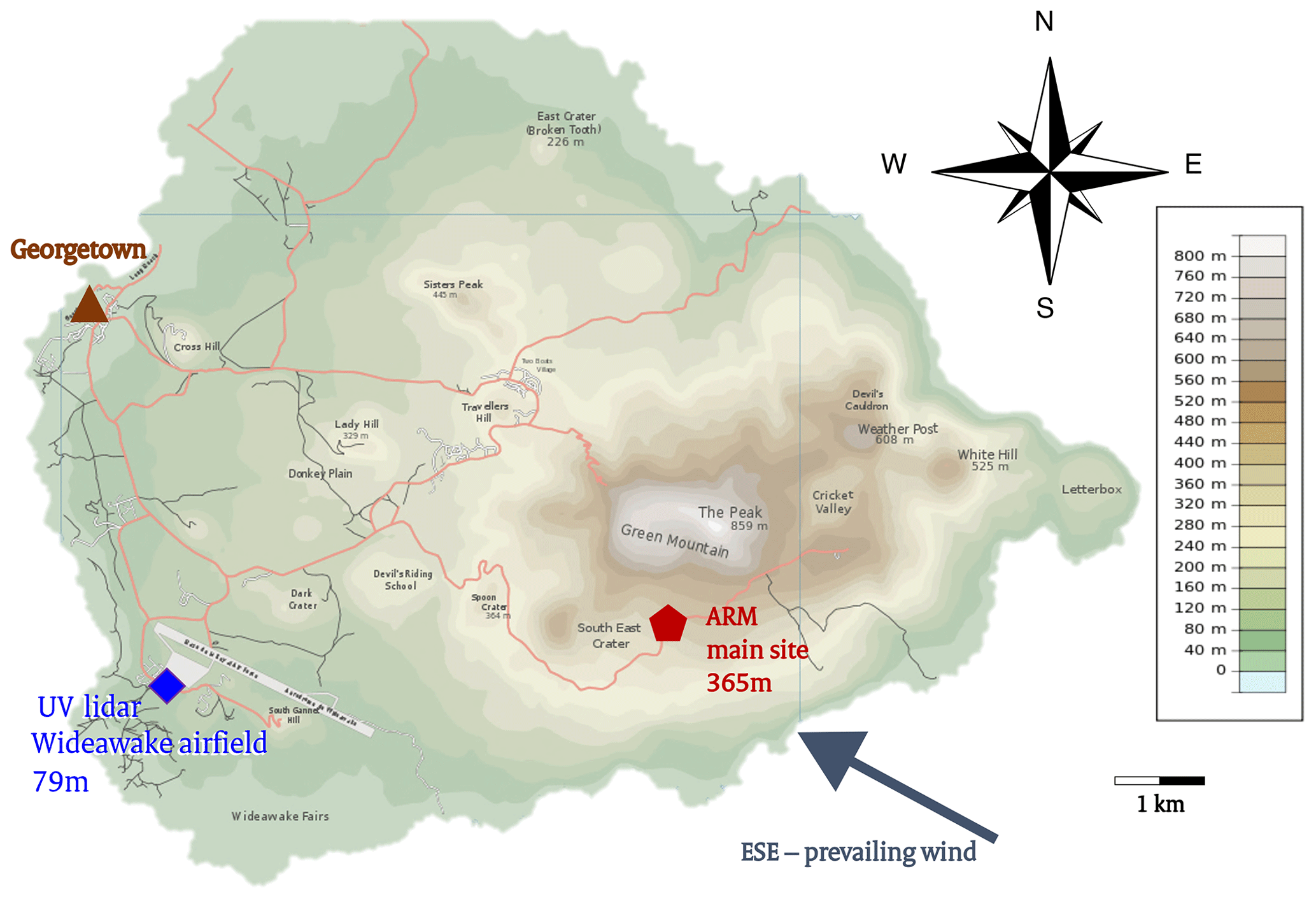
Figure 1 Map of Ascension Island, showing the topography and the location of the UV lidar on Wideawake airfield and the ARM main site. The distance between the sites is 6.3 km. Georgetown is the island's main settlement.

2 Measurement campaign

From 3–29 September 2016 and from 15 August to 9 September 2017 the KNMI UV polarization lidar, normally located in Cabauw, the Netherlands, was relocated to Ascension Island, a remote volcanic island in the tropical Atlantic Ocean (8^∘ S, 14^∘ W). Ascension Island is located 1600 km from the African coast and 2250 km from the Brazilian coast. Its climate is a tropical desert, with temperatures ranging from 22 to 31 ^∘C and a low annual rainfall at an average of 142 mm (Dorman and Bourke, 1981), with the peak rainfall occurring in April. Ascension Island lies at the terminating stage of the SEAO SCT, with clouds capping the boundary layer at an altitude of around 1–2 km. The prevailing trade winds in the boundary layer are from the southeast (Kim et al., 2003) and mostly invariant. Above the boundary layer (>1200 m above sea level) the wind is coming from the equatorial regions and frequently loaded with suspended particles like smoke from African vegetation fires or desert dust (Swap et al., 1996; Miller et al., 2021).

The Ascension Island Initiative (ASCII) was aimed at identifying microphysical properties of marine low-level clouds in the presence of aerosols (Brown, 2016; Tenner, 2017; Schenkels, 2018). During the same time various other measurement campaigns were operated on and around Ascension Island, providing a myriad of complementary measurements. The ground-based campaign LASIC (Layered Atlantic Smoke Interactions with Clouds; Zuidema et al., 2016) operated a fully equipped ARM (Atmospheric Radiation Measurement) research facility in 2016 and 2017, while airborne measurements were provided in 2017 by CLARIFY-2017 (Haywood et al., 2021) and in 2016, 2017 and 2018 by ORACLES (ObseRvations of Aerosols above CLouds and their intEractionS; Redemann et al., 2021). On the African continent, in situ and airborne measurements of the smoke near the source were provided by the AEROCLO-sA (Aerosol Radiation and Clouds in southern Africa) campaign in Namibia (Formenti et al., 2019).

Figure 1 shows the main locations of the instruments used in this paper during the campaigns. The UV lidar was located on the southwestern side of the island throughout the 2016 and 2017 campaigns at Wideawake airfield, at 79 m above sea level. For all of 2016 and 2017, the ARM research facility was located on the southern slope of Green Mountain, at 365 m altitude and about 6.3 km from Wideawake airfield. This location, south of the 859 m peak of the volcanic island, ensured that pristine oceanic air would be sampled during the prevailing wind direction, which is east-southeast of the site. Radiosondes were launched from the airfield four times daily.

2.1 Lidar measurements

Lidar measurements have a long history of retrieving aerosol extinction and backscatter profiles in clear-sky scenes (e.g. Pappalardo et al., 2014). In aerosol conditions, the lidar signal is determined by single-scattering events. In clouds, multiple scattering must be considered. The occurrence of multiple scattering also has implications for the polarization state of the lidar signal. Since cloud droplets are spherical, under single-scattering conditions, the lidar return signal retains its polarization state. In clouds, multiple scattering becomes more and more important as the beam penetrates the cloud base and the lidar beam becomes increasingly depolarized. On Ascension Island, lidar measurements were performed to study both aerosol and cloud properties, using a commercial Leosphere ALS-450 lidar operating at 355 nm, with separate parallel and perpendicular channels. The data were acquired with a vertical resolution of 15 m and a temporal resolution of about 30 s. The field of view of the lidar was found to be between 0.5 and 1.5 mrad. The retrieval error in 2016 was 19.75 %, and in 2017 it was 39.05 %, due to the calibration, retrieval and measurement errors. In 2017, instrument internal misalignment (likely incurred during transport) resulted in a lower SNR and uncertain calibration. Therefore, 2016 data are used in this paper, except where noted. The lidar was operational 24 h d⁻¹ for almost the entire period of the campaign, except from 24 to 27 September 2016, due to power cuts on the airfield. Details about the calibration and the campaign can be found in Brown (2016), Tenner (2017) and Schenkels (2018).

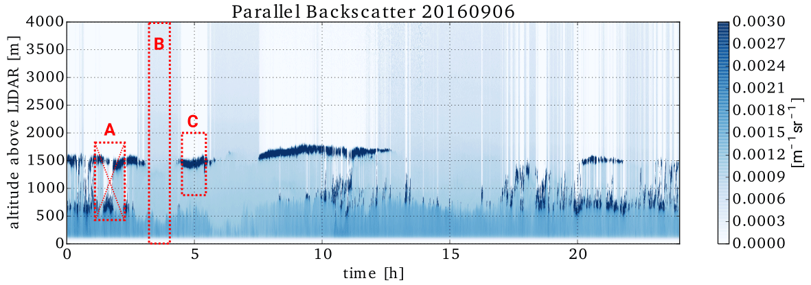
Figure 2 The parallel attenuated backscatter from the lidar on 6 September 2016. The red boxes show examples of selected data: (a) a cloud with varying cloud base and double cloud layers, not appropriate for analysis; (b) an appropriate selection of clear sky; and (c) an appropriate selection of a cloud. Please note that the date format in this figure is year month day.

An example of the type of both cloudy and clear-sky observation selected for analysis is presented in Fig. 2. The skies over Ascension Island are typically defined by broken low-level warm clouds interspersed with clear spells. The lidar measurements were used to estimate the aerosol and cloud properties during various circumstances, detailed below. Due to the strong background light from the overhead sun, the ability to observe aerosols was much better at night or when no clouds were present.

2.2 Aerosol optical thickness

Using cloud-free lidar observations, the daily averaged aerosol optical thickness (AOT) retrieved from the lidar during the 2016 campaign is shown in Fig. 3 and compared to AErosol RObotic NETwork (AERONET) measurements from the station located on Ascension Island at the ARM main site. AERONET offers quality-assured, cloud-screened automated direct sun measurements from ground-based, sun-tracking sun photometers every 15 min at eight wavelengths (Holben et al., 1998). The measurements at 340 nm were used here. The AERONET AOT data at this wavelength have an uncertainty of 0.021, due to atmospheric pressure variations assuming a 3 % maximum deviation from the mean surface pressure (Eck et al., 1999). The uncertainty in the lidar retrieval, taking into account the systematic error arising from the definition of the extinction-to-backscatter ratios and the random error due to the definition of the normalization height, was estimated to be about 11 % (Schenkels, 2018).

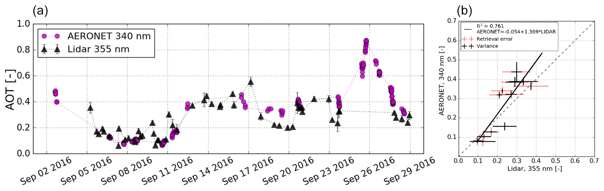
Figure 3 Aerosol optical thickness retrievals from AERONET at 340 nm compared to the retrieval from the UV lidar at 355 nm. (a) The daily averaged AERONET AOT (purple dots) during the 2016 campaign and the AOT from the lidar (black triangles), with black error bars showing the standard deviation. The retrieval uncertainties were 0.021 for AERONET and 11 % for the lidar data. (b) A scatterplot of the measurements on the left, with black bars showing the variances and red bars showing the retrieval errors. Pearson's correlation coefficient was 0.761. The dashed line is the 1:1 line, and the full black line is a linear least-squares fit with a slope of 1.369 and offset of −0.054. Please note that the date format in this figure is month day year.

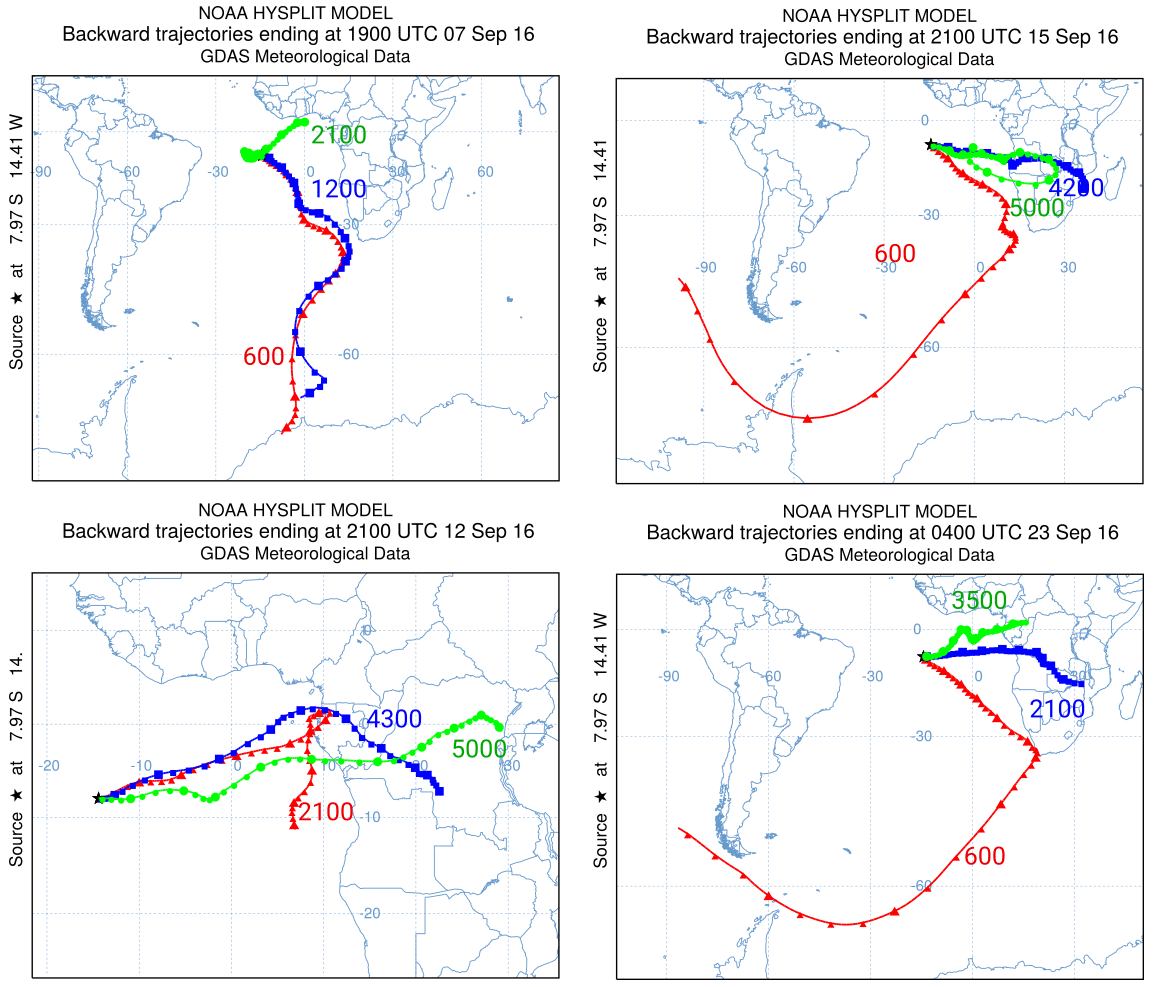
Figure 4 Example back trajectories during the 2016 ASCII measurement campaign on 7, 12, 15 and 23 September 2016. All trajectories were run for 240 h and ended over Ascension Island at different heights, as shown by the altitude (in m). The figures show the stable MBL east-southeast flow and the advection of air from the African continent, except on 7 September 2016. GDAS: Global Data Assimilation System. Please note that the date format in this figure is day month year.

Daily averaged retrievals were compared for cloud-free periods for each instrument. Since the instruments were not at the same position, the cloud-free periods can differ. However, the AOT distribution is assumed to be spatially consistent on the spatial scale of around 6 km. The comparison between the AERONET and lidar retrieved AOT is good, with a correlation coefficient of 0.76.

The daily averaged AOT measurements show low aerosol conditions during the beginning of the campaign until 11 September 2016 and increasing values until 17 September 2016. After 17 September the values decrease, although not to the same very low values as in the beginning of the month, and there are again higher values towards the end. On 25 and 26 September 2016, AERONET shows AOT values up to about 0.9, but unfortunately the lidar was not operational on those days. These values are consistent with 500 nm AERONET results, shown by Zuidema et al. (2018). AOT at 500 nm peaked in August 2016 and returned to low background values in the beginning of September 2016, as does the AOT at 340 nm. The increase in AOT over Ascension Island from 14–17 and 23–26 September 2016 is consistent with the increase in strength of the southern African easterly jet, which develops from being weak in the beginning of September 2016 to being strong at the end of the month (Ryoo et al., 2022). This promoted the advection of black carbon (BC) from the African continent over the SEAO, suggesting that the AOT over Ascension Island increased due to the advection of smoke from Africa. This was also checked by the inspection of daily backscatter trajectories, showing advection of air in the free troposphere directly from the east during the days with increased AOT (e.g. 13–17 and 23–26 September) but not during low-AOT episodes (e.g. 6–10 September 2016). A few example back trajectories during different episodes of the campaign are shown in Fig. 4.

3 Aerosol–cloud interactions

Aerosol–cloud interactions were determined from the lidar measurements using the 2016 data only. In 2017, alignment issues resulted in a lower SNR and large uncertainties, and these data were discarded for the analyses in this section. Three approaches are presented. First, a simple comparison of days of low and high aerosol concentration is made, showing the change in cloud parameters. Next, the aerosol indirect effect was determined following the metrics developed in Feingold et al. (2001) and McComiskey et al. (2009): the aerosol–cloud interaction (ACI) is quantified, for a constant ambient relative humidity, by a change in cloud parameters due to a change in the number of available condensation nuclei. For the cloud effective radius,

$$\begin{array}{}\text{(1)}& {\mathrm{ACI}}_{\mathrm{r}}=-{\displaystyle \frac{\mathrm{d}\ln R_{\mathrm{eff}}}{\mathrm{d}\ln A}},\end{array}$$

and for the cloud droplet number density,

$$\begin{array}{}\text{(2)}& {\mathrm{ACI}}_{\mathrm{N}}={\displaystyle \frac{\mathrm{d}\ln N_{\mathrm{d}}}{\mathrm{d}\ln A}}.\end{array}$$

In these equations A is the aerosol proxy, which should represent the aerosol abundance, and can be aerosol extinction, aerosol optical thickness or another aerosol quantity.

This approach was applied in two ways: first, by using the daily averaged AOT around the cloud base and comparing it to the cloud parameters, which are also determined around the cloud base (since the lidar does not penetrate deep into the cloud), and second, by determining the aerosol abundance below the cloud, using the lidar-derived aerosol extinction profile below the clouds. Hence, in the first method the aerosol proxy is determined during cloud-free spells, while in the second method the aerosol proxy is determined during cloudy spells, i.e. collocated in time with the cloud parameter retrievals. Aerosol optical thickness was retrieved using the classical Klett–Fernald two-mode method, i.e. applying Eqs. (A8) and (A9) to clear-sky measurements and cloud droplet number density, with the effective radius being retrieved by applying Eqs. (A12) and (A13) to measurements during cloudy periods.

3.1 Classification

A first coarse indication of the change in cloud properties can be obtained from a comparison of periods with a high aerosol loading over Ascension Island, compared to periods with low aerosol loading, assuming everything else will be the same. A classification of the 2016 measurements was made after defining periods of clear-sky and cloudy periods for each day with broken clouds, by visual inspection of the lidar quicklooks (Tenner, 2017).

A classification was made of days when aerosols were expected to mix with the clouds and days when the aerosol loading was particularly low. Figure 5 explains the logic: two layers were discriminated, one from 850 to 2150 m altitude, which was assumed to be the altitude of the clouds, and one from 2150 to 5000 m, which was defined as the free troposphere. If the AOT in both layers was low (below 0.07 was chosen), the day was assigned the label “clean”; if the AOT in the layer between 850 and 2150 m was high (higher than 0.07), the day was assigned the label “mixed”. If the AOT was high only in the free troposphere, the day was labelled “separated” and not considered, which happened in one case. The average aerosol optical thickness was determined during the cloud-free periods (10 during clean days and 17 during mixed days), and the average cloud properties were determined during the cloudy periods (6 during clean days and 31 during mixed days).

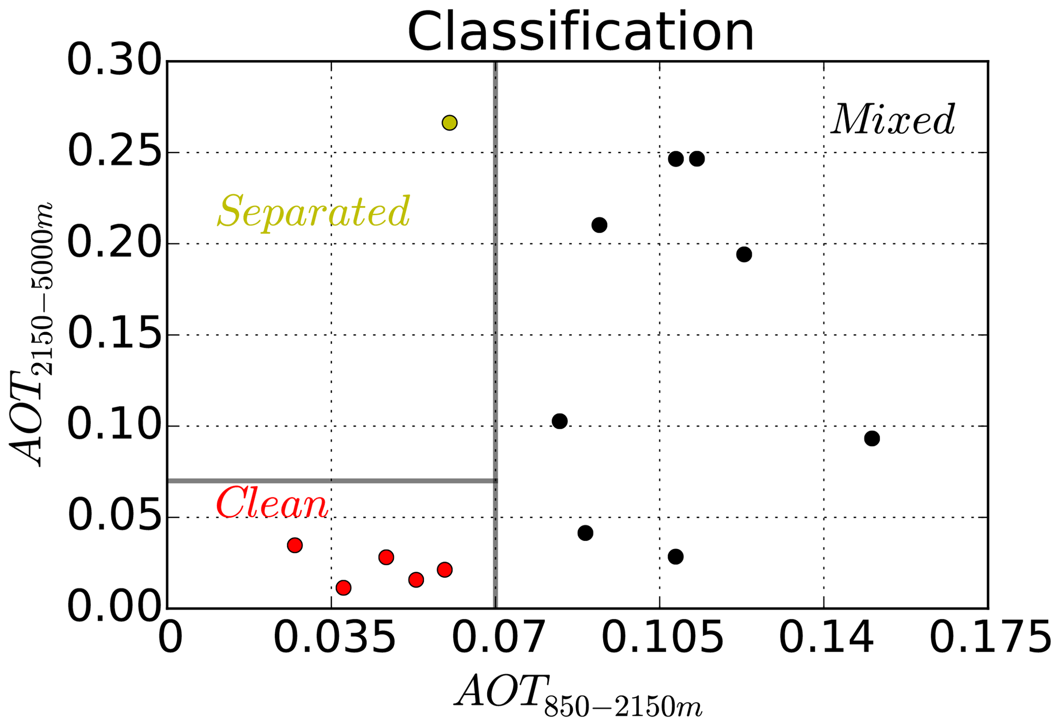
Figure 5 Classification of the average clear-sky AOT during broken cloud days, at two levels: from 850 to 2150 m, which is assumed to be at the cloud level, and from 2150 to 5000 m, which is assumed to be in the free troposphere above the clouds.

Using this crude selection of cases resulted in a clear difference in the average cloud properties between the different days, as shown in Fig. 6. The cloud droplet number density N_d was 294 ± 91 cm⁻³ during all clean days, doubling to over 611 ± 191 cm⁻³ during the mixed days. Conversely, $R_{\mathrm{eff}}^{\mathrm{100}}$ was reduced from 3.81 ± 0.6 to 2.85 ± 0.2 µm. This suggests a change to smaller, more numerous cloud particles with the availability of a larger number of cloud condensation nuclei. However, the assumption that the humidity does not change cannot be guaranteed with such an approach.

Figure 6 The mean value of (a) the cloud droplet number density N_d and (b) the cloud effective radius at the reference height $R_{\mathrm{eff}}^{\mathrm{100}}$ for the clean and mixed cases. The black error bar represents the standard deviation; the grey bars represent the sample standard deviation.

3.2 Aerosol–cloud interactions around the cloud base

Next, the ACI was computed using AOT from the daily averaged extinction profile as before but now averaged from 300 m below the cloud base until 1000 m above the cloud base. This level was chosen to isolate the MBL aerosol impact on cloud droplets near the cloud base, the region that the lidar is sensitive to. For each cloudy period the cloud properties were determined as before and used in Eqs. (1) and (2) to quantify the ACI. The results are shown in Fig. 7. The points were fitted weighted by the associated standard deviation, yielding ACI_N = 0.3 ± 0.21 for the cloud droplet number density and ACI_r = 0.18 ± 0.06 for the cloud effective radius. ACI_r is at the high end of values found by previous studies. For example, McComiskey et al. (2009) found values of ACI_r ranging from 0.0–0.16 in marine stratus clouds, while Kim et al. (2008) found values from 0.04–0.17 in continental stratus. Higher values (0.13–0.19) were found in the Arctic (Garrett et al., 2004) and for very large ranges of aerosol concentration including strong pollution (0.21–0.33) (Ramanathan et al., 2001).

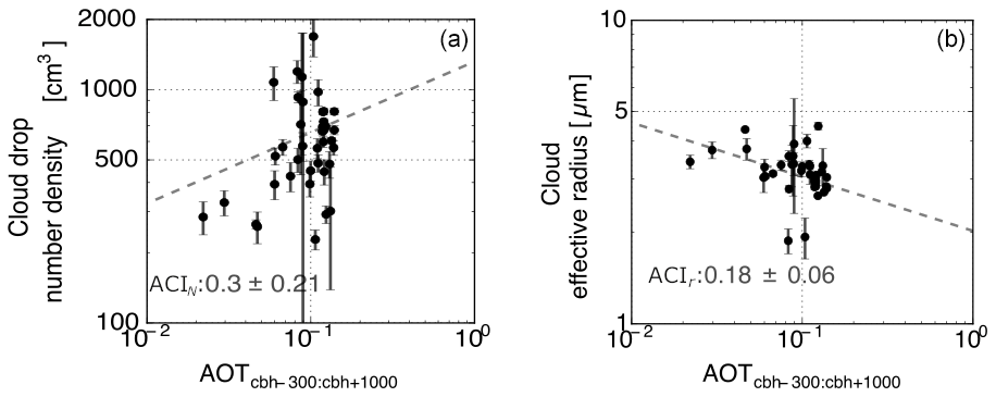
Figure 7 (a) Weighted mean of the cloud drop number density versus daily average AOT for each cloud selection. (b) Weighted mean of the cloud effective radius versus daily average AOT for each cloud selection. For both cloud properties a linear fit is plotted and the ACI is given. The standard deviation was used as weights in the fit.

3.3 Aerosols below the cloud

In order to get aerosol and cloud proxies closer together in time, ACI_r and ACI_N were also calculated using the aerosol extinction below the clouds during cloudy periods. For this, the aerosol extinction profile was computed using Eq. (A8) but with the normalization height set inside the cloud and the extinction-to-backscatter ratio set to 20 sr in the cloud and 50 sr below the cloud, as described in Sect. A3.2. Furthermore, the cloud extinction-to-backscatter ratio was corrected for multiple scattering using Eq. (A10). The extinction profile was determined from 200 m above the lidar to avoid overlap until 300 m below the cloud base to avoid the mixing region of wet aerosols just below the cloud. The mean aerosol extinction coefficient was used instead of the AOT because the height of the range bins changed per cloud selection. Cloud retrievals of 30 s intervals were averaged, with a minimum of 3 values and a maximum of 24 values, corresponding to cloud periods of 1.5 to 12 min. The errors from the lidar inversion were used as weights in the determination of the ACI values. The results for the 2016 measurements are plotted in Fig. 8.

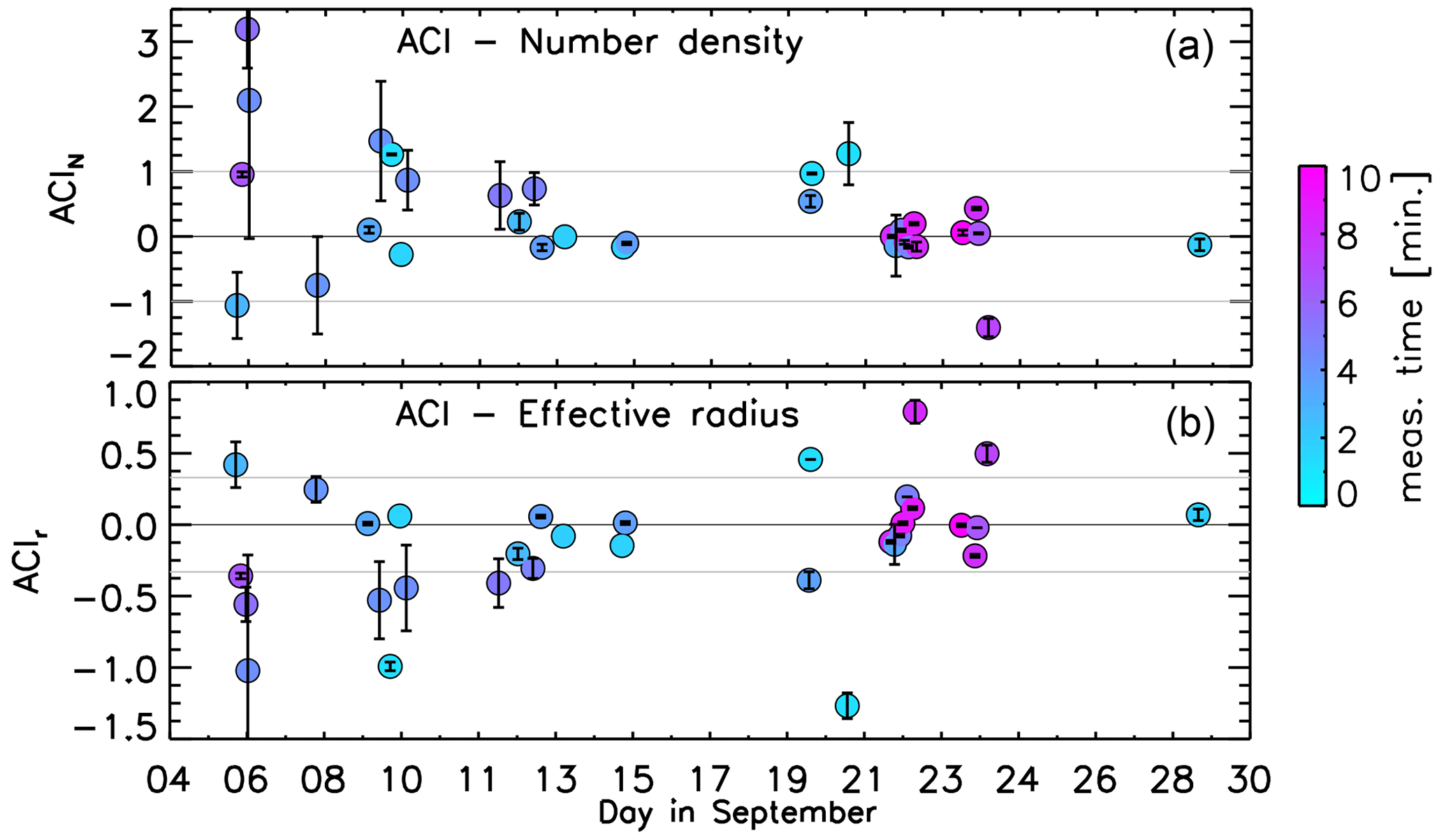
Figure 8 Aerosol–cloud interaction (ACI) for each selected cloud period in September 2016, using the average aerosol extinction profile below a cloud and (a) the retrieved cloud droplet number density and (b) the retrieved cloud droplet effective radius. The error bars indicate the standard deviation of the measurements during each selected interval; the colours indicate the duration of the intervals. The horizontal grey lines indicate the physically feasible bounds of the ACI values.

The ACI for all cloud periods during the 2016 campaign show varying results. Many values are beyond the theoretically feasible values, indicated in the plots by the horizontal grey lines. Theoretically, the absolute value $|\mathrm{ACI}{|}_{\mathrm{N}}$ must be below 1 and the absolute value $|\mathrm{ACI}{|}_{\mathrm{r}}$ must be below 0.33 (McComiskey et al., 2009), reaching the maximum absolute values if all aerosol particles are activated to droplets. However, a number of retrievals show much larger values, characterized by large uncertainties. The theoretical numbers are based on idealized clouds in a constant atmospheric state. The retrievals with large numbers and large uncertainties must be associated with variable meteorological conditions that drive the changes in cloud and aerosol properties, like a co-varying liquid water path (LWP). Furthermore, the theoretical bound for ACI_N is based on aerosol number; using a mean extinction coefficient below clouds may lead to values larger than 1.

Around 12–15 and 21–24 September ACI_N and ACI_r are mostly within the physical ranges with small uncertainties. These episodes correspond to periods of increased AOT over Ascension Island (see Fig. 3). This suggests that during those periods the interaction of smoke with the cloud base is the driving mechanism for forming more numerous, smaller droplets.

4 Discussion

The three presented methods all suggest some indication of the Twomey effect in the cumulus clouds around Ascension Island in 2016 during various episodes. However, changing meteorological conditions could affect the results. An inspection of (back)trajectories during the measurement period showed that the MBL around Ascension Island is very persistent (cf. Fig. 4). Daily back trajectories of air ending at 600 m altitude over Ascension Island invariably showed MBL air being transported from the southeast with little to no vertical displacement for all the days during the 2016 campaign, indicating a stable of moist well-mixed air in the MBL as expected over this region. On the other hand, the air transported to the cloud layer, e.g. at 2100 m altitude, was from the east most of the time (loaded with smoke) but was also from the west and variable.

In a recent paper, Ryoo et al. (2022) show that during September 2016 the southern African easterly jet increases develops from being weak in the beginning of September 2016 to being strong at the end of the month, with increased relative humidity and BC concentrations over the central southern Atlantic Ocean at 600 hPa especially around 15–17 and 27 September 2016. These episodes correspond to the increased AOT in Fig. 3, showing the dominance of the large-scale circulation in the free troposphere on the AOT fluctuation over Ascension Island. However, the correlation between BC concentration and relative humidity can also explain a positive correlation between the AOT and cloud droplet number density, as observed in Figs. 6 and 7, if more particles become activated with more available moisture. However, in that case the observed reduction in the cloud effective radius is unlikely, and we conclude that the advection of smoke from the African continent reduces the effective cloud droplet size at the cloud base through the first aerosol indirect effect.

4.1 Cloud parameters

Lidar retrievals of the cloud parameters have been performed in only a few cases before (Donovan et al., 2015; Sarna and Russchenberg, 2016; Jimenez et al., 2020). Below, the cloud retrievals from the UV polarization lidar are compared to retrievals from cloud radars located at the ARM research facility. Unfortunately, in 2016 the cloud radar was operational only for a short period during the campaign, so 2017 data are also used to assess the cloud data from the lidar retrievals.

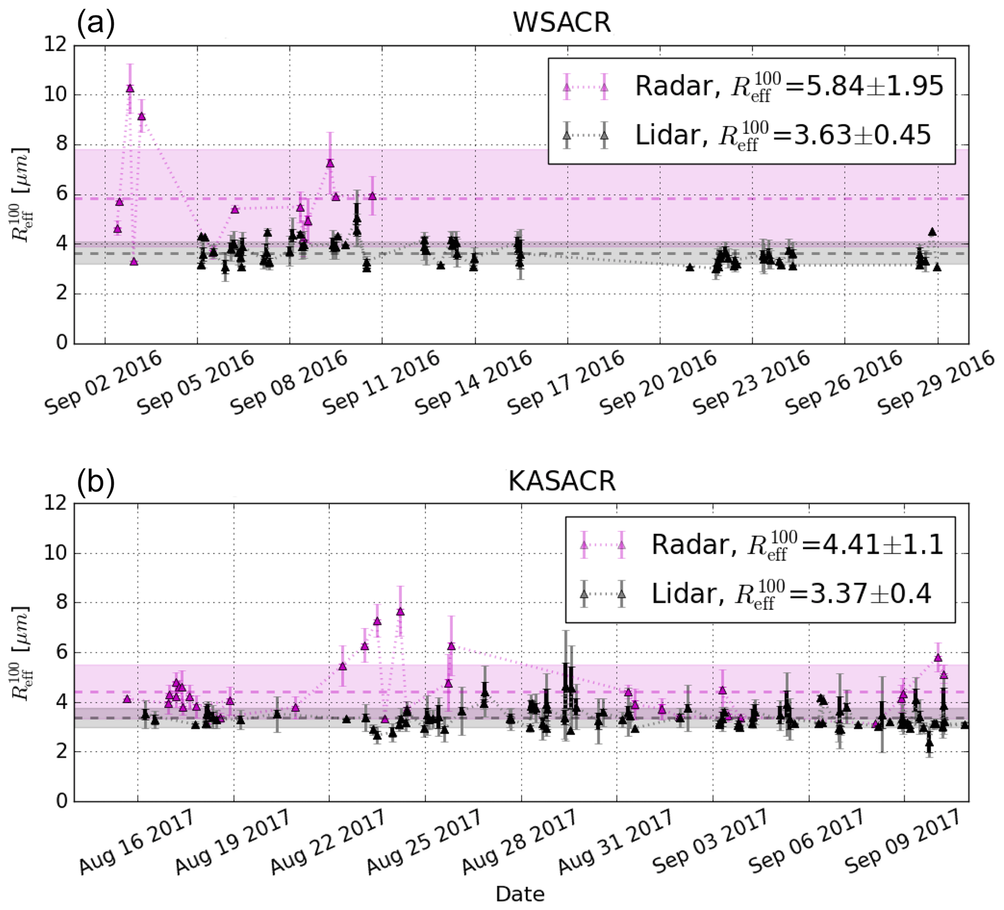
Figure 9 $R_{\mathrm{eff}}^{\mathrm{100}}$ for selected cloud periods in (a) 2016 and (b) 2017 from the lidar (grey) and the cloud radar (purple). The shading shows the standard deviation or retrieval error, while the variance in the cloud per measurement period is given by the error bars. The dashed line gives the mean $R_{\mathrm{eff}}^{\mathrm{100}}$. Please note that the date format in this figure is month day year.

In 2016, the W-Band Scanning ARM Cloud Radar (WSACR) was operated from the start of the lidar measurement period until 11 September. In 2017, the Ka-Band Scanning ARM Cloud Radar (KASACR) was operated during the entire period of the lidar operation. WSACR was operated at a frequency of 94 GHz, and KASACR was operated at 35.3 GHz. Both radars have a field of view of 0.3^∘. Although the radars were operated with scanning strategies, here only the vertical pointing modes were used, taken each hour for a duration of 4 min. The 2D radar reflectivity factor Z, with a time resolution of 2 s and a vertical resolution of 30 m, was collected from the ARM website.

The radar reflectivity was used to derive $R_{\mathrm{eff}}^{\mathrm{100}}$ following the method described by Frisch et al. (1995). Assuming a cloud with a lognormal droplet size distribution,

$$\begin{array}{}\text{(3)}& n\left(r\right)={\displaystyle \frac{N_{\mathrm{d}}}{\sqrt{\mathrm{2}\mathit{\pi }}r{\mathit{\sigma }}_x}}\exp \left({\displaystyle \frac{-\left(\ln \right(r)-\ln (R_{\mathrm{0}}){)}^{\mathrm{2}}}{\mathrm{2}{\mathit{\sigma }}_x^{\mathrm{2}}}}\right),\end{array}$$

where is R₀ the median radius, σ_x is the spread of the lognormal distribution, the effective cloud droplet radius R_eff is related to the median radius by

$$\begin{array}{}\text{(4)}& R_{\mathrm{eff}}=R_{\mathrm{0}}\exp \left({\displaystyle \frac{\mathrm{5}}{\mathrm{2}}}{\mathit{\sigma }}_x^{\mathrm{2}}\right),\end{array}$$

and the radar reflectivity is

$$\begin{array}{}\text{(5)}& Z={\mathrm{2}}^{\mathrm{6}}{N}_{\mathrm{d}}{R}_{\mathrm{0}}^{\mathrm{6}}\exp \left(\mathrm{18}{\mathit{\sigma }}_x^{\mathrm{2}}\right).\end{array}$$

This gives a relationship for the effective cloud droplet radius of

$$\begin{array}{}\text{(6)}& R_{\mathrm{eff}}\left(z\right)={\displaystyle \frac{\mathrm{1}}{\mathrm{2}}}{\left({\displaystyle \frac{Z\left(z\right)}{N_{\mathrm{d}}}}\right)}^{\mathrm{1}/\mathrm{6}}\exp (-\mathrm{0.5}{\mathit{\sigma }}_x^{\mathrm{2}}),\end{array}$$

and the value of $R_{\mathrm{eff}}^{\mathrm{100}}$ to be compared to the lidar retrievals is simply given by the above equation with z corresponding to 100 m above the cloud base with the cloud base supplied by co-located lidar ceilometer measurements (see Appendix B). The value for σ_x was set to 0.34 ± 0.09, which is a typical value for marine, low-level clouds (Fairall et al., 1990; Frisch et al., 1995; Miles et al., 2000). An uncertainty of ±3 dBZ in the reflectivity factor was used to compute the error margins. N_d can be estimated from the lidar inversions (see Eq. A11). Daily averaged lidar estimates of N_d were around 466 ± 127 cm⁻³ in 2016 and 540 ± 142 cm⁻³ in 2017. The uncertainty in retrieved N_d is between 25 % and 50 % (Donovan et al., 2015). The lidar estimates of N_d are higher than earlier reported values of 100 ± 70 cm⁻³ for marine, low-level clouds (Davidson et al., 1984; Martin et al., 1994) and used by Frisch et al. (2002). However, N_d is seasonally dependent, with higher values in the boreal summer over SEAO (Li et al., 2018) and the western northern Atlantic Ocean (Dadashazar et al., 2021), and Eq. (6) shows that relatively large changes in N_d will produce only small changes in R_eff. The use of the literature value of 100 cm⁻³ in the radar estimates increased the effective radius by about 3 µm.

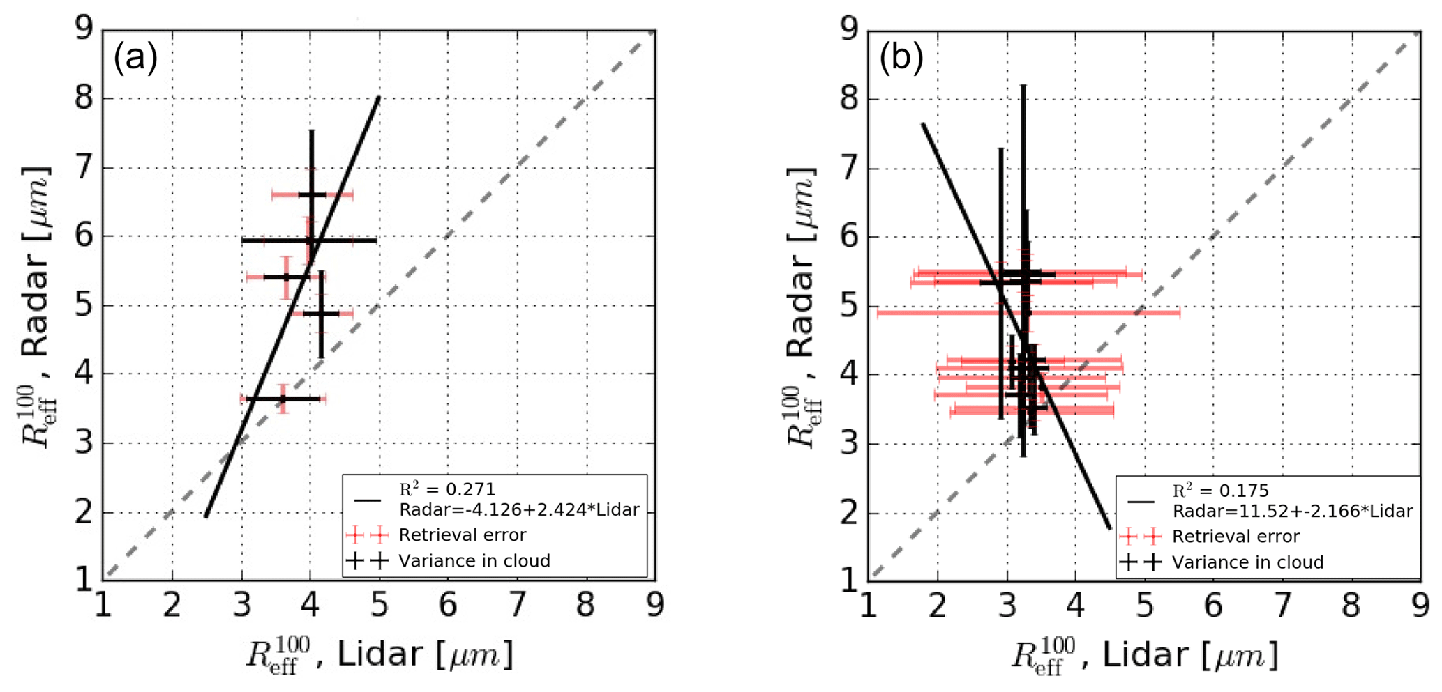
Figure 10 Comparison of daily averaged $R_{\mathrm{eff}}^{\mathrm{100}}$ from lidar and cloud radar in (a) 2016 and (b) 2017. The retrieval error is shown by the red error bars, while the variance of the daily measurements is shown by the black error bars. The dashed line shows the 1:1 line, and the full black line is a linear least-squares fit. The slope and offset of the fit are indicated in the legend, along with Pearson's correlation coefficient.

$R_{\mathrm{eff}}^{\mathrm{100}}$ estimates from lidar and cloud radar are compared in Figs. 9 and 10. Figure 9 shows the lidar retrievals for selected cloud periods, with the variance in the measurements shown by error bars and the estimated measurement error shown by the shaded purple (radar) and grey (lidar) areas. The average retrieved effective droplet radii (shown by the dashed lines) was 3.63±0.45 µm in 2016 and 3.37±0.4 µm in 2017 for the lidar retrieval and 5.84±1.95 µm in 2016 and 4.41±1.1 µm in 2017 for the radar retrievals. Figure 10 shows scatterplots of the daily averaged retrievals of $R_{\mathrm{eff}}^{\mathrm{100}}$ from lidar and radar retrievals in 2016 and 2017. In general, the estimates of $R_{\mathrm{eff}}^{\mathrm{100}}$ from the cloud radar are larger than from the lidar. This will be even larger for lower values for N_d. The comparison is complicated by the low number of measurements in 2016. In 2017, the average value is closer, but the alignment problems complicates the comparison, and no correlation was found between the radar and lidar estimates.

The dependence on the assumed value of N_d can be removed altogether using cloud liquid water path (LWP) data from a microwave radiometer (MWR) (Frisch et al., 2002). An MWR was operated at 23.8 and 31.4 GHz alongside the WSACR until 11 September 2016. The radar–MWR method described in (Frisch et al., 2002) was also applied in addition to the radar-only (Frisch et al., 1995) method. The radar–MWR method, however, tended to yield particle size measurements much higher than the radar-only approach. Moreover, the radar–MWR results tended to yield $R_{\mathrm{eff}}^{\mathrm{100}}$ values strongly inconsistent with non-drizzling clouds (e.g. values greater than 15 µm) and unrealistically low values of number density (e.g. less than 5 cm⁻³). The reason for this is unclear but may point to biases in the LWP data used or an error in the implementation.

The differences in the effective-radius retrieval could be the consequence of a number of factors. Both the radar-only and radar–MWR methods are sensitive to the presence of drizzle, while the lidar-only method is relatively insensitive to the presence of drizzle (Donovan et al., 2015). Even small amounts of drizzle may result in radar-reflectivity-based retrievals overestimating cloud particle sizes (e.g. Fox and Illingworth, 1997; Küchler et al., 2018; Wang and Geerts, 2003). It should be noted, however, that the smaller effective radius seen with lidar is consistent with that reported by Jimenez et al. (2020) (e.g. Fig. 6). Also, Conant et al. (2004) report cloud droplet effective radii from cloud radar measurements in warm cumulus clouds growing from about 2 µm near the cloud base to 10 µm at 1000 m above the cloud base. Frisch et al. (2002) report radar estimates of $R_{\mathrm{eff}}^{\mathrm{100}}$ in stratus clouds ranging from 4 to 8 µm in close agreement with aircraft measurements, depending strongly on cloud height.

5 Conclusions

In this study, aerosol–cloud interactions were studied in the broken cloud deck over Ascension Island during the African monsoonal dry season in 2016 and 2017, which is about July to October. During these months, plumes of smoke from vegetation fires drift over the ocean. The typical clouds over Ascension Island are cumulus clouds at the terminating stage of the stratocumulus-to-cumulus (SCT) transition. Smoke affects this transition is various ways. We found that the presence of smoke decreases the cloud droplet sizes near the cloud base and increases the cloud droplet number density, likely due to the first aerosol indirect effect. On average, the cloud drop number density was 294 ± 91 cm⁻³ and the cloud effective radius was 3.81 ± 0.6 µm during smoke-free days, compared to 611 ± 191 cm⁻³ and 2.85 ± 0.2 µm during days with smoke at cloud level. Similarly, aerosol–cloud interactions were quantified using cloud base parameters during cloud periods and daily averaged AOT at cloud level: the cloud droplet number density ACI_N was 0.3 ± 0.21, and the cloud effective radius ACI_r was 0.18 ± 0.06.

Lastly, aerosol and cloud properties were retrieved simultaneously by the lidar during cloudy periods. This was possible by retrieving aerosol extinction profiles under the clouds. During two episodes, 12–15 September 2016 and 20–24 September 2016 an indirect effect was found, corresponding to periods with increased transport of air from the African continent over the SEAO. This increased not only the BC concentration and AOT over Ascension Island but also the relative humidity. However, the results show a decrease in droplet size and increase in droplet number density near the cloud base related to increases in aerosol concentration, suggesting that the smoke is responsible for more numerous but smaller cloud droplets, which will shorten the SCT, both by warming the MBL during the day and by making cloud droplets more susceptible to evaporation.

The lidar retrieved values of the effective radius were small compared to many other studies of cloud droplet sizes of warm low-level clouds (e.g. Gupta et al., 2022). However, lidar estimates of the cloud droplet effective radius are restricted to cloud base values, and care should be taken when comparing estimates from ground-based radars and satellite retrievals. Vertical profiles of R_eff are typically strongly growing from a few micrometres to over 10 µm and more until the cloud top. A radar beam can penetrate the cloud completely, and the average retrieved effective radius depends on the assumed vertical distribution. Satellite retrievals of cloud droplet sizes are typically biased to the cloud top retrievals. Therefore, comparisons between these types of retrievals should be performed only when corrected for the vertical profile of the cloud droplet sizes (Zhang et al., 2011). A comparison with radar estimates of droplet sizes near the cloud base showed consistent values to within the measurement uncertainties.

This is the first time a UV polarization lidar was used to determine cloud parameters at the cloud base of marine cumulus clouds in the SCT zone over the SEAO. The measured depolarization of the lidar beam was fitted to lookup tables (LUTs) of precalculated depolarization by cloud droplets using Monte Carlo (MC) simulations, relating the depolarization to the cloud droplet effective radius and the cloud extinction parameter at a reference height using a proper cloud model. This method shows potential for the monitoring of aerosol–cloud interactions at strategically positioned locations in climate sensitive areas, like the SEAO. The simultaneous retrievals of aerosol extinction and cloud properties from one single instrument can be helpful in the measurement of aerosol indirect effects, which constitutes the largest uncertainties in global climate models. However, we found that proper calibration of the instrument and careful selection of the data are essential.

Appendix A: Theory

The theory of the applied methods has been described in earlier papers cited in the text. For completeness, the method applied to the UV lidar data on Ascension Island is described below.

A1 UV lidar

The total power returned to a lidar by backscattering in the atmosphere under single-scattering conditions is

$$\begin{array}{}\text{(A1)}& P\left(z\right)={\displaystyle \frac{C_{\mathrm{lid}}}{z^{\mathrm{2}}}}{\mathit{\beta }}_{\mathit{\pi }}\left(z\right)\exp \left(-\mathrm{2}\underset{\mathrm{0}}{\overset{z}{\int }}\mathit{\alpha }\left(z^{\prime }\right)\mathrm{d}{z}^{\prime }\right),\end{array}$$

where P is the power received by the instrument, z is the altitude from the instrument along the line of sight, C_lid is the lidar calibration coefficient, α is the atmospheric extinction coefficient and β_π is the atmospheric backscatter coefficient. The atmospheric extinction and backscatter coefficients can be divided into a molecular, aerosol and cloud part, viz.

$$\begin{array}{}\text{(A2)}& \begin{array}{r}\mathit{\alpha }={\mathit{\alpha }}_{\mathrm{m}}+{\mathit{\alpha }}_{\mathrm{a}}+{\mathit{\alpha }}_{\mathrm{c}},\\ {\mathit{\beta }}_{\mathit{\pi }}={\mathit{\beta }}_{\mathrm{m}}+{\mathit{\beta }}_{\mathrm{a}}+{\mathit{\beta }}_{\mathrm{c}}.\end{array}\end{array}$$

The extinction-to-backscatter ratio (or lidar ratio) S is defined as $S\left(z\right)=\mathit{\alpha }/\mathit{\beta }$. The aerosol scattering ratio (R_asca) is defined as $R_{\mathrm{asca}}=({\mathit{\beta }}_{\mathrm{a}}+{\mathit{\beta }}_{\mathrm{m}})/{\mathit{\beta }}_{\mathrm{m}}$, which is 1 if there are no aerosols.

A2 Molecular scattering

The molecular backscatter coefficient can be calculated using (Collis and Russel, 1976)

$$\begin{array}{}\text{(A3)}& {\mathit{\beta }}_{\mathrm{m}}={\displaystyle \frac{{\mathit{\rho }}_{\mathrm{air}}}{M}}{\left({\displaystyle \frac{\mathit{\lambda }}{\mathrm{550}}}\right)}^{-\mathrm{4.09}}{\mathrm{10}}^{-\mathrm{32}}{\mathrm{m}}^{-\mathrm{1}}{\mathrm{sr}}^{-\mathrm{1}},\end{array}$$

where λ is the wavelength; M is the average molecular mass of air ($\mathrm{4.81}\times {\mathrm{10}}^{-\mathrm{26}}$ kg); and the atmospheric density was determined using

$$\begin{array}{}\text{(A4)}& {\mathit{\rho }}_{\mathrm{air}}={\displaystyle \frac{p}{T}}{\displaystyle \frac{\mathrm{1}}{{\mathrm{R}}_{\mathrm{dry}\mathrm{air}}}},\end{array}$$

where p is the measured pressure, T is the measured temperature and R_dry air is the gas constant for dry air with an average value of 287 J kg⁻¹ K⁻¹. The temperature and pressure were determined from radiosondes, launched four times daily from Ascension Island. The molecular extinction coefficient α_m can be calculated using the molecular extinction-to-backscatter ratio $S_{\mathrm{mol}}=\mathrm{8}\mathit{\pi }/\mathrm{3}$ sr (Guzzi, 2008). At the lidar wavelength of 355 nm molecular scattering is strong, and this was used to calibrate the lidar. Details can be found in Schenkels (2018).

A3 AOT retrieval

For a lidar operating in the UV, molecular scattering is strong and must be accounted for in the inversion. In this case, a two-mode method following e.g. Klett (1981) and Fernald (1984) can be applied using the transformed variables (Sarna et al., 2021)

$$\begin{array}{}\text{(A5)}& P^{\prime }\left(z\right)=S\left(z\right)P\left(z\right)\exp \left(\mathrm{2}\underset{\mathrm{0}}{\overset{z}{\int }}{\mathit{\alpha }}_{\mathrm{m}}\left(z^{\prime }\right)-S\left(z^{\prime }\right){\mathit{\beta }}_{\mathrm{m}}\left(z^{\prime }\right)\mathrm{d}{z}^{\prime }\right)\end{array}$$

and

$$\begin{array}{}\text{(A6)}& {\mathit{\alpha }}^{\prime }\left(z\right)=\left(S\left(z\right){\mathit{\beta }}_m\left(z\right)+{\mathit{\alpha }}_a\left(z\right)\right).\end{array}$$

Now Eq. (A1) can be rewritten as

$$\begin{array}{}\text{(A7)}& P^{\prime }\left(z\right)={\displaystyle \frac{C_{\mathrm{lid}}}{z^{\mathrm{2}}}}{\mathit{\alpha }}^{\prime }\left(z\right)\exp \left(-\mathrm{2}\underset{\mathrm{0}}{\overset{z}{\int }}{\mathit{\alpha }}^{\prime }\left(z^{\prime }\right)\mathrm{d}{z}^{\prime }\right),\end{array}$$

with the analytical solution

$$\begin{array}{}\text{(A8)}& {\mathit{\alpha }}^{\prime }\left(z\right)=\left[{\displaystyle \frac{\frac{P^{\prime }\left(z\right)z^{\mathrm{2}}}{P^{\prime }\left(z_{\mathrm{0}}\right)z_{\mathrm{0}}^{\mathrm{2}}}}{\frac{\mathrm{1}}{{\mathit{\alpha }}^{\prime }\left(z_{\mathrm{0}}\right)}+\mathrm{2}{\int }_z^{z_{\mathrm{0}}}\frac{P^{\prime }\left(z\right)z^{\mathrm{2}}}{P^{\prime }\left(z_{\mathrm{0}}\right)z_{\mathrm{0}}^{\mathrm{2}}}\mathrm{d}{z}^{\prime }}}\right],\end{array}$$

where z₀ is a normalization height. From the transformed variable α^′, the aerosol extinction is derived to be ${\mathit{\alpha }}_{\mathrm{a}}\left(z\right)={\mathit{\alpha }}^{\prime }\left(z\right)-S\left(z\right){\mathit{\beta }}_{\mathrm{m}}\left(z\right)$. The aerosol backscatter coefficient is now derived by dividing the aerosol extinction by the height-dependent lidar ratio. The aerosol optical thickness (τ) of a layer can be obtained by integrating the aerosol extinction profile over the altitude of the layer:

$$\begin{array}{}\text{(A9)}& \mathit{\tau }(z_{\mathrm{1}};z_{\mathrm{2}})=\underset{z_{\mathrm{1}}}{\overset{z_{\mathrm{2}}}{\int }}{\mathit{\alpha }}_{\mathrm{a}}\left(z\right)\mathrm{d}z.\end{array}$$

A3.1 Cloud-free scenes

In clear-sky scenes the normalization height is set to an altitude at which the aerosol extinction is 0. From literature (e.g. Wandinger et al., 2016; Greatwood et al., 2017) and from observations on the island, it was concluded that marine aerosols are always present in the lower boundary layer, up until 1200 m. S_marine was set to be 25 sr, a good approximation for marine aerosols (Wandinger et al., 2016; Cattrall et al., 2005; Müller et al., 2007); (aged) smoke and dust were often, almost always, present above the boundary layer, in the layer from 1200 to 5000 m, sometimes mixed in the boundary layer. For this layer the lidar ratio S_dark was set to 50 sr (Wandinger et al., 2016). Above 5000 m, the air was mostly clean and clear of aerosols and the lidar ratio reduces to the molecular extinction-to-backscatter ratio defined above. The normalization height was set to 7 km. Various tests were performed varying S_marine and S_dark around their values of 25 and 50 sr to check the sensitivity of the choices, resulting in 5 % changes in AOT within the expected reasonable ranges of S.

A3.2 Aerosol below clouds

In order to derive aerosol optical thickness close to clouds, aerosol extinction profiles were retrieved for cloudy scenes under the clouds, using Eq. (A8). However, in this case the normalization height is not located at an altitude without aerosols but rather inside the cloud, where the aerosol contribution can be neglected. The normalization height was determined by the cloud base height and the cloud extinction. The extinction-to-backscatter ratio was set to 20 sr in the cloud and 50 sr below the cloud (Wandinger et al., 2016).

Furthermore, multiple scattering, which influences the lidar return and the cloud extinction, should be taken into account in a cloud. Therefore, the cloud extinction-to-backscatter ratio, used to determine α^′ in Eq. (A8), was corrected by a multiple scattering correction factor η:

$$\begin{array}{}\text{(A10)}& S_{\mathrm{c}}={\displaystyle \frac{(\mathrm{1}-\mathit{\eta }){\mathit{\alpha }}_{\mathrm{c}}}{{\mathit{\beta }}_{\mathrm{c}}}}.\end{array}$$

The correction factor η was determined from a sensitivity study over 3 d in 2016 with broken clouds. Aerosol profiles below clouds during these days were fitted to aerosol retrievals during clear-sky spells close in time on these days. The correction factor was varied between 0.3 and 0.5 in steps of 0.05, resulting in overcorrection and undercorrection. The best fit was found for 0.35 and 0.4. The difference in aerosol extinction coefficient at an altitude of 300 m below the cloud base between η=0.35 and 0.4 is about $\mathrm{2.6}\times {\mathrm{10}}^{-\mathrm{5}}$ m⁻¹. In all subsequent processing a value of η=0.4 was used. See Tenner (2017) for details.

A4 Clouds

Although the lidar equation (Eq. A1) formally only applies for single scattering, the derivation of cloud extinction and backscatter coefficient in this section is based on a polarization change after multiple scattering, first developed by Donovan et al. (2015). Light returning from a liquid cloud will be partially depolarized due to multiple scattering by the cloud droplets (Liou and Schotland, 1971). This multiple scattering in a liquid water cloud can be simulated by a Monte Carlo (MC) model, assuming a cloud model. This was achieved using the Earth Clouds and Aerosol Radiation Explorer (EarthCARE) simulator (ECSIM) lidar-specific MC forward model. The ECSIM lidar MC model is a modular multi-sensor simulation framework, which was used to calculate the spectral-polarization state of the lidar signal.

The underlying cloud model is based on clouds with a linear liquid water content (LWC) profile from the cloud base and a constant cloud droplet number density (N_d) (e.g. de Roode and Los, 2008). Various MC simulations were carried out for different LWC slopes, number densities and lidar fields of view, and cloud base values. The MC results were then used to produce lookup tables which form the basis of a forward model which is fast enough to serve as the forward retrieval model in an optimal-estimation retrieval procedure. Details are described in the remainder of this section.

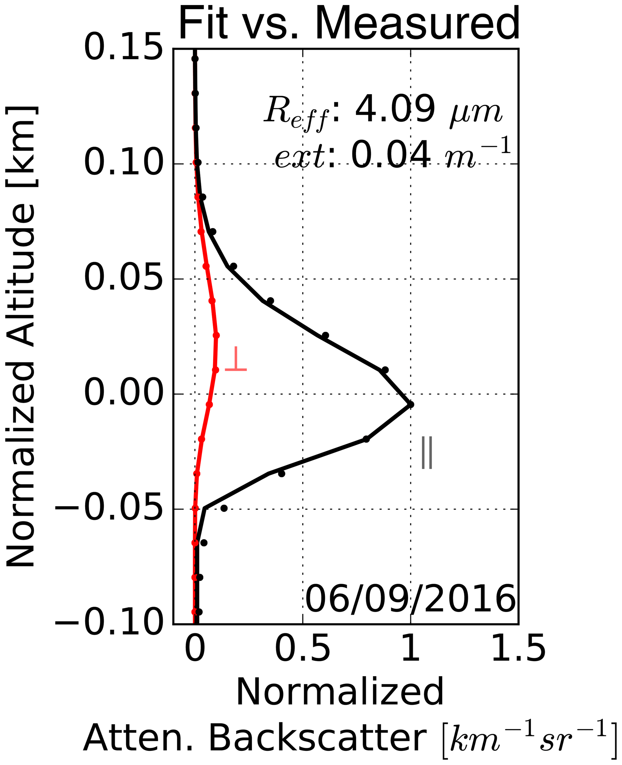
Figure A1 Measured (solid line) and fitted (dots) vertical profiles for the parallel attenuated backscatter (black) and perpendicular attenuated backscatter (red) on 6 September 2016 for the selected cloud (C) in Fig. 2. Please note that the date format in this figure is day month year.

The cloud droplet size distribution was defined as a single-mode modified gamma distribution (Miles et al., 2000):

$$\begin{array}{}\text{(A11)}& n\left(r\right)={\displaystyle \frac{N_{\mathrm{d}}}{R_{\mathrm{m}}}}{\displaystyle \frac{\mathrm{1}}{(\mathit{\gamma }-\mathrm{1})\mathrm{!}}}{\left({\displaystyle \frac{r}{R_{\mathrm{m}}}}\right)}^{\mathit{\gamma }-\mathrm{1}}\exp \left({\displaystyle \frac{r}{R_{\mathrm{m}}}}\right),\end{array}$$

where N_d is the cloud droplet density, defined to be constant with height; r is the droplet radius; R_m is the mode radius; and γ is the shape parameter of the distribution.

A linear liquid water content defines a constant liquid water lapse rate, Γ_l. When the liquid water content increases with height and the number density remains constant, the cloud droplet effective radius, defined as

$$\begin{array}{}\text{(A12)}& R_{\mathrm{eff}}={\displaystyle \frac{\int n\left(r\right)r^{\mathrm{3}}\mathrm{d}r}{\int n\left(r\right)r^{\mathrm{2}}\mathrm{d}r}},\end{array}$$

will increase with height. The cloud extinction coefficient α_c also increases with height. This leads to the prediction that the depolarization ratio is generally increasing throughout the cloud, while observations show that the depolarization ratio may exhibit a peak (Sassen and Petrilla, 1986). Furthermore, the model represents semi-infinite clouds, with a cloud top at infinity. However, the lidar signal can only penetrate a few hundred metres into the cloud. Therefore, no information is known about the upper part of the cloud, and any retrieved parameters are only applicable to the cloud base region; the parameters were calculated for a reference height. In this research, 100 m above the cloud base was assumed. This simple but effective cloud representation reduces the parameters to describe the cloud to two, the cloud extinction ${\mathit{\alpha }}_{\mathrm{c}}^{\mathrm{100}}$ at the reference height and the cloud effective radius $R_{\mathrm{eff}}^{\mathrm{100}}$ at the reference height.

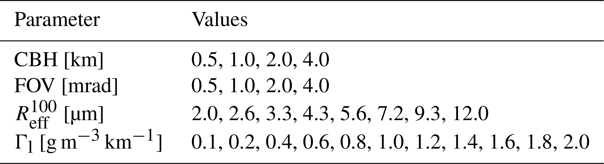
MC model simulations were performed for various values of the cloud base height (CBH), the lidar field of view (FOV), $R_{\mathrm{eff}}^{\mathrm{100}}$ and the adiabatic cloud base liquid water lapse rate Γ_l. The values are replicated from (Donovan et al., 2015) in Table A1. Lookup tables (LUTs) were generated from the simulations and predefined input parameters, the lidar constants, and initial values for $R_{\mathrm{eff}}^{\mathrm{100}}$ and ${\mathit{\alpha }}_{\mathrm{c}}^{\mathrm{100}}$. These LUTs contain information on the simulated parallel and perpendicular attenuated backscatter and therefore the depolarization ratio.

Table A1 Range of parameters used in the ECSIM MC calculations.

The observed attenuated backscatter and depolarization ratio were compared to the LUTs to find the best matching values for $R_{\mathrm{eff}}^{\mathrm{100}}$ and ${\mathit{\alpha }}_{\mathrm{c}}^{\mathrm{100}}$, by iteratively minimizing a cost function (Rodgers, 2000). In Fig. A1, the observed and fitted attenuated backscatter profiles from the LUTs are shown, for a cloud selected on 6 September 2017. The dotted lines correspond to the fitted values from the LUTs, with the parallel attenuated backscatter in black, the perpendicular attenuated backscatter in red. The observed profiles are represented by the corresponding solid lines.

The cloud drop number density N_d follows from the cloud effective radius and the cloud extinction of

$$\begin{array}{}\text{(A13)}& N_{\mathrm{d}}={\mathit{\alpha }}_{\mathrm{c}}^{\mathrm{100}}{\displaystyle \frac{\mathrm{1}}{\mathrm{2}\mathit{\pi }}}{\displaystyle \frac{\mathrm{1}}{(R_{\mathrm{eff}}^{\mathrm{100}}{)}^{\mathrm{2}}}}{\displaystyle \frac{\mathrm{1}}{k}},\end{array}$$

where k is 0.75±0.15.

Because multiple scattering occurs in a cloud, the LUTs, the shape of the attenuated backscatter and the depolarization ratio profiles are all well-defined functions of the LWC and effective radius profile. For single scattering the parallel attenuated backscatter profile will not depend on the effective radius profile.

It is important to note that the CBH is difficult to define from real observation due to the presence of sub-cloud drizzle and the presence of growing aerosol particles. The MC-based inversion results would be very sensitive to the absolute calibration of the attenuated backscatter if the CBH is used as a reference. Therefore, the peak of the observed parallel lidar attenuated backscatter is used as a reference instead of the CBH in the fitting procedure. Consequently, the CBH is produced as a byproduct, and in Appendix B the derived CBH will be compared to observations of the CBH using different instruments.

Appendix B: Cloud base height validation

It is important to compare the cloud parameters from the lidar and the cloud radars at the same relative height, since the effective radius strongly depends on the height in the cloud. The effective radius was determined at a reference of 100 m above the cloud base height (CBH), which was related to the peak of the observed parallel lidar attenuated backscatter. The accuracy of the backscatter peak as the CBH cannot directly be compared to the CBH from the cloud radar because of the different locations of the instrument. The effect of the spatial distance between the instruments was investigated by comparing the CBH from two ceilometers that were installed in the airport and the ARM main site. This is illustrated in the left panel of Fig. B1 for the day of 26 August 2017. The CBHs from these instruments, relative to the mean sea level, are highly correlated in general (Pearson's correlation coefficient was 0.931). However, on average a higher cloud fraction was found over the ARM main site compared to the airport, due to the higher elevation of the site. More low-level clouds were detected over the ARM main site, and the cloud fraction differed. However, this should not affect the analyses too much, since the main difference is in the low-level clouds and the selected cloud periods had CBHs higher than 1000 m.

The CBHs from the lidar and from the ceilometer at the airport were compared, as shown in the right panel of Fig. B1. The correlation was higher than 90 %. Therefore, the relative height of the peak of the backscatter can be considered a good proxy for the relative position of the CBH.

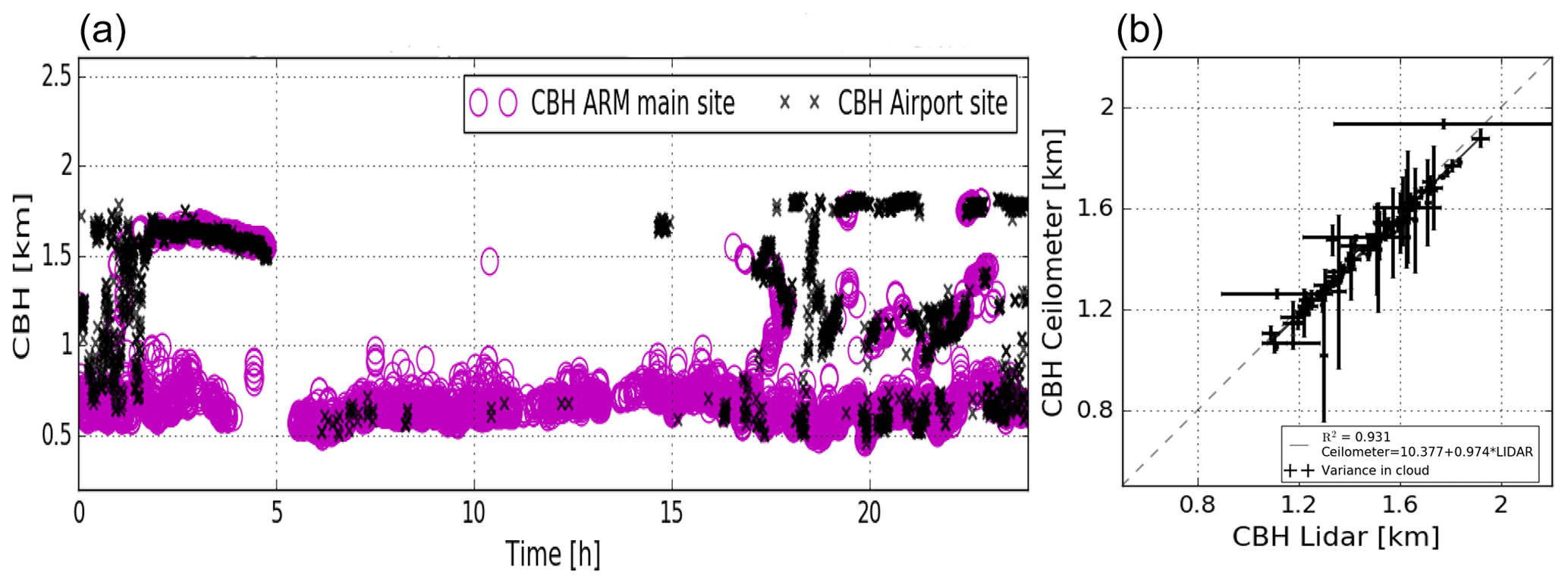
Figure B1 (a) The CBH from the ceilometer at the airport (black crosses, elevation of 79 m) compared to the CBH from the ceilometer at the ARM main site (purple circles, elevation of 365 m) on 26 August 2017. The CBH is measured relative to the mean sea level. (b) Comparison of the cloud base height determined from the UV lidar and the ceilometer located at the airport. The dashed line is the 1:1 line.