the Creative Commons Attribution 4.0 License.
the Creative Commons Attribution 4.0 License.
 | 11 May 2023
Technical note: Improving the European air quality forecast of the Copernicus Atmosphere Monitoring Service using machine learning techniques
Jean-Maxime Bertrand
Frédérik Meleux
Anthony Ung
Gaël Descombes
Augustin Colette
Model output statistics (MOS) approaches relying on machine learning algorithms were applied to downscale regional air quality forecasts produced by CAMS (Copernicus Atmosphere Monitoring Service) at hundreds of monitoring sites across Europe. Besides the CAMS forecast, the predictors in the MOS typically include meteorological variables but also ancillary data. We explored first a “local” approach where specific models are trained at each site. An alternative “global” approach where a single model is trained with data from the whole geographical domain was also investigated. In both cases, local predictors are used for a given station in predictive mode. Because of its global nature, the latter approach can capture a variety of meteorological situations within a very short training period and is thereby more suited to cope with operational constraints in relation to the training of the MOS (frequent upgrades of the modelling system, addition of new monitoring sites). Both approaches have been implemented using a variety of machine learning algorithms: random forest, gradient boosting, and standard and regularized multi-linear models. The quality of the MOS predictions is evaluated in this work for four key pollutants, namely particulate matter (PM10 and PM2.5), ozone (O3) and nitrogen dioxide (NO2), according to scores based on the predictive errors and on the detection of pollution peaks (exceedances of the regulatory thresholds). Both the local and the global approaches significantly improve the performances of the raw ensemble forecast. The most important result of this study is that the global approach competes with and can even outperform the local approach in some cases. This global approach gives the best RMSE scores when relying on a random forest model for the prediction of daily mean, daily max and hourly concentrations. By contrast, it is the gradient boosting model which is better suited for the detection of exceedances of the European Union regulated threshold values for O3 and PM10.
- Article
(3604 KB) - Full-text XML
- BibTeX
- EndNote


Outdoor air pollution induced by natural sources and human activities remains a major environmental and health issue worldwide. Producing reliable short-term forecasts of pollutant concentrations is a key challenge to support national authorities in their duties regarding the European Air Quality Directive, like planning and communications about the air quality status towards the general public in order to limit the exposure of populations. Progress in computing technologies during the last decades has allowed for the rise of large-scale chemistry transport models (CTMs) which provide a comprehensive view of the air quality on a given time period and geographical domain by solving the differential equations that govern the transport and transformation of pollutants in the atmosphere. An overview of such deterministic air quality forecasting systems operating in Europe was provided by Zhang et al. (2012). Ensembles of several CTMs have also been used in order to improve single-model forecasts (Delle Monache and Stull, 2003; Wilczak et al., 2006). Such an ensemble approach is currently used in the frame of the Copernicus Atmospheric Monitoring Service (Marécal et al., 2015) to provide daily air quality forecasts over the European territory (https://atmosphere.copernicus.eu/air-quality, last access: 13 April 2023).
Statistical post-processing offers a way to improve the raw outputs of deterministic models while not undermining inherent capacities of CTMs. For instance, one must acknowledge that regional-scale CTMs are primarily designed to capture background air pollution so that spatial representativeness remains a concern in the immediate vicinity of large emission sources. Spatial downscaling is therefore a good example of the relevance of hybrid statistical and deterministic modelling, but correction of systematic biases and better modelling of extreme values can also be achieved at the deterministic model's grid scale. Modellers are working to solve such issues by continuously improving models and input data, but post-processing offers a pragmatic solution that must be considered.
Running-mean bias correction, Kalman filter and analogues (Delle Monache et al., 2006; Kang et al., 2008; Djalalova et al., 2015) are the most widespread examples of model output statistics (MOS) proposed in the literature to improve air quality forecasts. Another very common type of MOS is multi-linear regression statistical modelling to predict a corrected concentration at a given location using any available information, including the deterministic forecast, meteorological variables or any other ancillary data. Such regression-based MOS approaches have been implemented in Europe in several national air quality forecasting services, sometimes for more than a decade such as in the French operational forecasting system PREV'AIR (Honoré et al., 2008; Rouïl et al., 2009). More recently, Petetin et al. (2022) performed a systematic evaluation of one of the most exhaustive selections of MOS techniques (including Kalman filter and analogues in addition to tree-based machine learning algorithms) for the specific case of ozone forecasts in the Iberian Peninsula.
The goal of this work is to explore the use of several machine learning algorithms to improve the air quality forecasts of the CAMS regional ensemble model at hundreds of monitoring sites across Europe for the ozone (O3), particulate matter (PM10 and PM2.5) and nitrogen dioxide (NO2) pollutants. The classical MOS approach consists of building an individual model at each monitoring site using local data. In this context, some MOS methods (including those based on machine learning algorithms) need long training periods, based on model outputs and observations, to reach optimized performances. The need for a long training period (with constant model formulation over this period) is a difficulty for the maintenance of operational MOS systems since the evolution of pollutant emissions, the upgrades of the deterministic model and the addition of new monitoring sites require frequent recalibrations of the MOS. This issue is particularly pertinent in our context since, as a regularly maintained operational model, the CAMS ensemble model (composed of seven members during the period of study) is subject to frequent upgrades. Every year there are between one and two upgrades to the set-up of the CAMS individual models producing air quality forecasts at regional scale over Europe. Therefore, an alternative global approach, building one single model for all the monitoring sites with a very short training period (a few days preceding the forecast), but using data from the whole geographical domain was also tested for comparison. In the following article, we present first, in Sect. 2, the observations and model datasets used to train and test the predictive models. Then, MOS approaches and algorithms are presented in Sect. 3. Finally, Sect. 4 explores the sensitivity of the two MOS approaches to training data, and Sect. 5 compares and discusses their performances in the frame of the selected scenarios.
The MOS development is based on 3 years of air pollution and meteorological data covering the 2017–2019 period. These data include hourly in situ observations of PM10, PM2.5, NO2 and O3 concentrations at hundreds of urban, suburban and rural background regulatory monitoring stations and is retrieved from the up-to-date (UTD) dataset of the Air Quality E-reporting database (https://www.eea.europa.eu/data-and-maps/data/aqereporting-9, last access: 13 April 2023) of the European Environment Agency. Daily mean, daily 1 h maximum and daily 1 h minimum were calculated when 75 % of the hourly data were available for the considered dates (i.e. at least 18 h over 24 h). All the stations located in the European region, over a domain ranging from −25∘ W to 45∘ E longitude and from 30∘ S to 70∘ N latitude, have been considered in this work. The total numbers of stations available for training and testing the MOS are 1535 for O3, 957 for PM10, 1468 for NO2 and 498 for PM2.5.
Hourly concentrations from the CAMS European ensemble forecast have been retrieved from the Atmosphere Data Store (https://ads.atmosphere.copernicus.eu/cdsapp#!/home, last access: 13 April 2023). During the 2017–2019 period,1 the CAMS ensemble was defined as the median of seven individual models covering the European region at the resolution of 0.1∘ and developed by several European modelling teams, namely CHIMERE (Mailler et al., 2017), EMEP (Simpson et al., 2012), EURAD-IM (Hass et al., 1995), LOTOS-EUROS (Schaap et al., 2009), MATCH (Robertson et al., 1999), MOCAGE (Guth et al., 2016) and SILAM (Sofiev et al., 2015). Note that the CAMS ensemble was upgraded during the month of June 2019 with the use of a new anthropogenic emissions dataset, extension of the geographical domain, and provision of dust (within PM10) and secondary inorganic aerosols (aggregation of ammonium sulfates and nitrates within PM2.5) in near real-time production. The impact of this upgrade on the MOS will be discussed in the Conclusion section. Hourly surface meteorological data were interpolated from the IFS (Integrated Forecasting System2 – ECMWF). The specific list of meteorological variables is discussed in Sect. 3.3. Both concentration and meteorological forecasts were extracted at the locations of monitoring stations using a distance-weighted average interpolation.
The MOS strategy can be called “hybrid” modelling in the sense that it uses both a deterministic forecast (here the CAMS regional ensemble) and other relevant predictors to produce a statistically corrected output concentration. In machine learning terminology it corresponds to a supervised learning problem as we use a training dataset composed of a number of predictor variables (also called features) labelled with the corresponding pollutant concentration observations. The model fitted with the training data is then applied to future situations (new predictors values) to forecast pollutant concentrations. Three distinct problems have been considered in this work: prediction of daily mean, daily maximum and hourly concentrations. The quality of the predictions is explored for the first day (D+0) or first 24 h of the forecast in this work, but the methodologies proposed are adapted to tackle longer forecast leads.
3.1 Machine learning algorithms
Five types of predictive models based on different machine learning algorithms are tested and compared to each other. Three of them belong to the family of the linear models, namely the standard, the LASSO (least absolute shrinkage and selection operator) and the ridge linear model. They are formulated as Eq. (1):
where y∗ denotes the predicted value for the pollutant's concentration, α0 is the intercept term, xj denotes a continuous variable or a dummy variable (taking values of 0 or 1) that indicates the absence or presence of some categorical effect, αj represents the coefficients of the statistical model that have to be determined, and p is the number of predictors. The coefficients are chosen to minimize the penalized residual sum of squares (Eq. 2):
where yi denotes an observed concentration, and xij is the associated value for the predictor j; N is the number of observations in the training dataset; λ is a penalty coefficient; and f denotes either the absolute value or the square function. In the case where λ is set to zero, the regularization term on the rightmost part of the equation nullifies, and we obtain a standard linear model (LM) based on the minimization of residual sum of squares. Otherwise, λ will have to be tuned (see below), and depending on the choice of f – absolute value or square function – we obtain a LASSO or a ridge linear model, respectively. The ridge and the LASSO regressions were introduced separately by Hoerl and Kennard (1970) and Tibshirani (1996), respectively. For both the ridge and LASSO approaches, the regularization term in Eq. (2) favours solutions with coefficient values of small amplitude, thus reducing the risk of overfitting, i.e. of producing a model that sticks too close to the training data and has poor generalization skills. In contrast to the ridge regularization, the LASSO tends to produce exactly zero values for those coefficients associated with the less important predictors, offering a way to deal with variable selection and improving model interpretability. In this study, we used the implementation of the ridge and LASSO regression in the “glmnet” package in the R language (Friedman et al., 2010).
The other two predictive models are based on the decision trees described by Breiman et al. (1984). These trees are based on a series of nodes that represent both a predictor and an associated threshold value. Each node is divided into two subsequent nodes until we reach a final node (a leaf) that gives the value of the prediction. The prediction function can also be seen as a partition of the predictors space where each sub-region is associated with a constant output value. Decision trees are an interesting solution as they can capture complex non-linear interactions and internally handle the selection of relevant predictors. However, they suffer from poor generalization skills. To tackle this issue, ensemble methods based on an aggregation of decision trees have been proposed. In this work we have tested two popular tree-based ensemble algorithms, namely the random forest (RF) and the gradient boosting model (GBM). RF models were introduced by Breiman (2001). They rely on an aggregation of binary decision trees that are built independently, using a bootstrap sample of the training data and randomly selecting subsets of candidate predictors at each node. The RF prediction is then given by the average of the trees predictions for regression problems or using majority vote for classification problems. Unlike random forest, GBM relies on relatively small trees that are built sequentially. After the first tree is trained, each subsequent tree is trained to predict the error left by the already trained ensemble of trees. When the final number of trees is reached, the GBM prediction is given by the sum of the initial concentration prediction and errors predicted by each tree. This mechanism, called “boosting”, was first described by Freund and Schapire (1996) with the adaBoost algorithm for the prediction of a binary variable. The “gradient boosting machine” algorithm is an adaptation, from Friedman (2001), for the prediction of quantitative variables. In this study we used the “randomForest” (Liaw and Wiener, 2002) and “gbm” (Greenwell et al., 2019) R packages for the implementation of the RF and GBM algorithms, respectively.
A key challenge with statistical learning methods is to learn as much as possible from the training data, without losing generalization skills. To reach an optimal balance and optimize the predictive performances, a learning algorithm may be tuned by choosing values for some parameters often referred to as hyper-parameters. The method used for tuning these hyper-parameters consists of a grid search, where possible values for each hyper-parameter are predefined. A model is trained and tested for every possible combination of hyper-parameter value using a fivefold cross-validation procedure. The best combination of hyper-parameter is then selected to train the final model but this time using the full training dataset. The tuning of these hyper-parameters is performed at every monitoring site for the local MOS approach or every day for the global MOS approach (local and global approaches are defined in Sect. 3.2). The number of parameters to be tuned depends on the algorithm. It is limited to one for the LASSO and ridge model, two for the random forest model, and four for the GBM model. To limit the number of combinations and computation time, the grids of possible values for each parameter were kept simple, with very few values to test, and remained the same in all the learning configurations of this study. The grids of tuning values for each algorithm are described in Appendix A. The tuning of the learning algorithms was performed using the caret R package (Kuhn, 2008).
3.2 Local and global approaches
The first approach tested in this work is local, meaning that a different MOS model is built for each observation station. This approach is implemented, for example, in the French national forecasting system PREV'AIR (Honoré et al., 2008). As each model is trained with local data only, we expect that it will be able to correct the deterministic model output in a way that reflects local specificities contributing to the station representativeness. A limitation of this local approach (referring to the methods computing a dedicated model per station) is that it often requires long time series of model output and observations (with constant model formulation and set-up over this period) to build an optimized predictive model at each observation site. Any upgrade of the modelling system that might sensitively impact the model behaviour and performances might lead to a deterioration of the MOS performances and thereby requires resource consuming for rerunning simulations with a consistent set-up over past periods in order to build updated MOS. Newly installed observation stations will not be integrated into the MOS until enough data are gathered to train a robust model (typically at least a full year). Moreover, this local approach is optimized if the conditions (model set-up, input data) during the predictions remain close to those of the training period. In practice this might not be the case, e.g. because of a drastic reduction of pollutant emissions due to local action plans or even not anticipatable circumstances such as the drop in activity induced by the COVID crisis. In such situations, the local MOS correction might be biased due to inadequacy with the training period's conditions. This feature is interesting and has been exploited, for example, to assess the impact of COVID-19 lockdown upon NO2 pollution in Spain (Petetin et al., 2020) based on a business-as-usual concentration correction, following the meteorological normalization method by Grange et al. (2018). However, there is also a need for more flexible MOS approaches that rapidly adapt to unanticipated changes in emissions. In the present study, the local approach was investigated using 2017 and 2018 data for training the MOS and using 2019 data to evaluate its performances.
The second approach, called “global”, has been designed to address operational constraints such as the CTMs upgrades or changes in the network or observations. The idea is to build a single global model with data coming from the whole set of observation stations. Even if a single model is derived for Europe, it is subsequently used in predictive mode with local predictors for each station. Because of their spatial distribution over the European domain, a large variety of meteorological situations can be captured within a relatively short (a few days) training period. Due to the seasonal variability, a new model must be trained regularly with the most recent data in order to remain close to new forecasting situations. In this study a new global model was trained every day using the last 3 d, the last 7 d or the last 14 d as training data and was applied to predict the concentrations of the upcoming day. This process was repeated 365 times to mimic an operational system running over the 2019 year period. With this global approach, any change in the CTM formulation will automatically be echoed in the MOS within a few days (depending on the choice for the training period duration). An important shortcoming of such a global approach is to ignore the local specificity in individual MOS models, whereas one of the main benefits of MOS approaches applied in addition to CTM results is precisely to remove systematic biases, i.e. induced by spatial representativeness limitation of the models. To tackle the varying spatial representativeness of the stations, the deterministic raw concentration output at each station was replaced by an “unbiased concentration” predictor, meaning the raw concentration minus the average error of the deterministic model at the station during the training period. As such, the global approach combines tree-based or regression machine learning algorithm and moving average (Petetin et al., 2022) unbiasing. This strategy will, for instance, lead to distinct MOS predictions at two stations with comparable meteorological and raw concentration forecasts (e.g. two stations located in the same grid cell). We also expect that this approach will better adapt to rapid changes in emissions induced by the situations mentioned above (e.g. pollution mitigation policies, COVID crisis).
3.3 Predictors
Increasing the number of predictors might improve the performances of a model but can also lead to overfitting and poor performances if not correctly handled by the machine learning algorithm. We have carried out tests with different sets of predictors in order to evaluate the risks and benefits from adding predictors depending on the machine learning algorithm considered. The following table (Table 1) details the sets of predictors that have been tested. These predictors fall into four categories: ensemble forecast, meteorological forecast, observations and other. MOS models have been trained to work both on an hourly basis and on a daily basis (to focus on the prediction of daily means or daily max). When designing an hourly model, all the quantitative predictors are hourly means, either forecasted for the considered time horizon (ensemble and meteorological forecasts) or observed during the previous day at the same time. The same model is used for every hour of the day, and the hour of the day is not explicitly passed to the model as a predictor (somehow considering that the other predictors provide enough information). When designing a daily model, a selection procedure is achieved before the training in order to choose (between the daily mean, daily min and daily max of each physical quantity) the one which is best correlated with the output variable. For both the local and global approaches, this correlation is calculated based on the full training dataset, meaning typically with 365 records for a local model built with a 1-year training dataset and 3000 records for a global model based on 1000 monitoring stations spread over the domain and a 3 d training period.
Set1 is the base set of predictors. It includes the ensemble forecasts (including the forecasts of the targeted pollutant and the three others), a first selection of surface meteorological variables (namely the temperature, relative humidity, zonal and meridional wind speed, and boundary layer's height) and observations of the previous day. The categorical day of week predictor was only used with the local approach which includes a long training period. For the global approach, tests have been performed using as a predictor either the raw ensemble (i.e. the median of the seven individual deterministic models) forecast or the unbiased ensemble concentration of the target pollutant. The unbiased concentration is defined as the forecasted ensemble concentration minus the bias observed at the station during the previous days (days of the chosen training period). Set2 includes set1 predictors plus four additional meteorological predictors, namely the short-wave radiation, the surface pressure, the cloud cover and precipitation.
Table 1Sets of predictors used in the MOS.
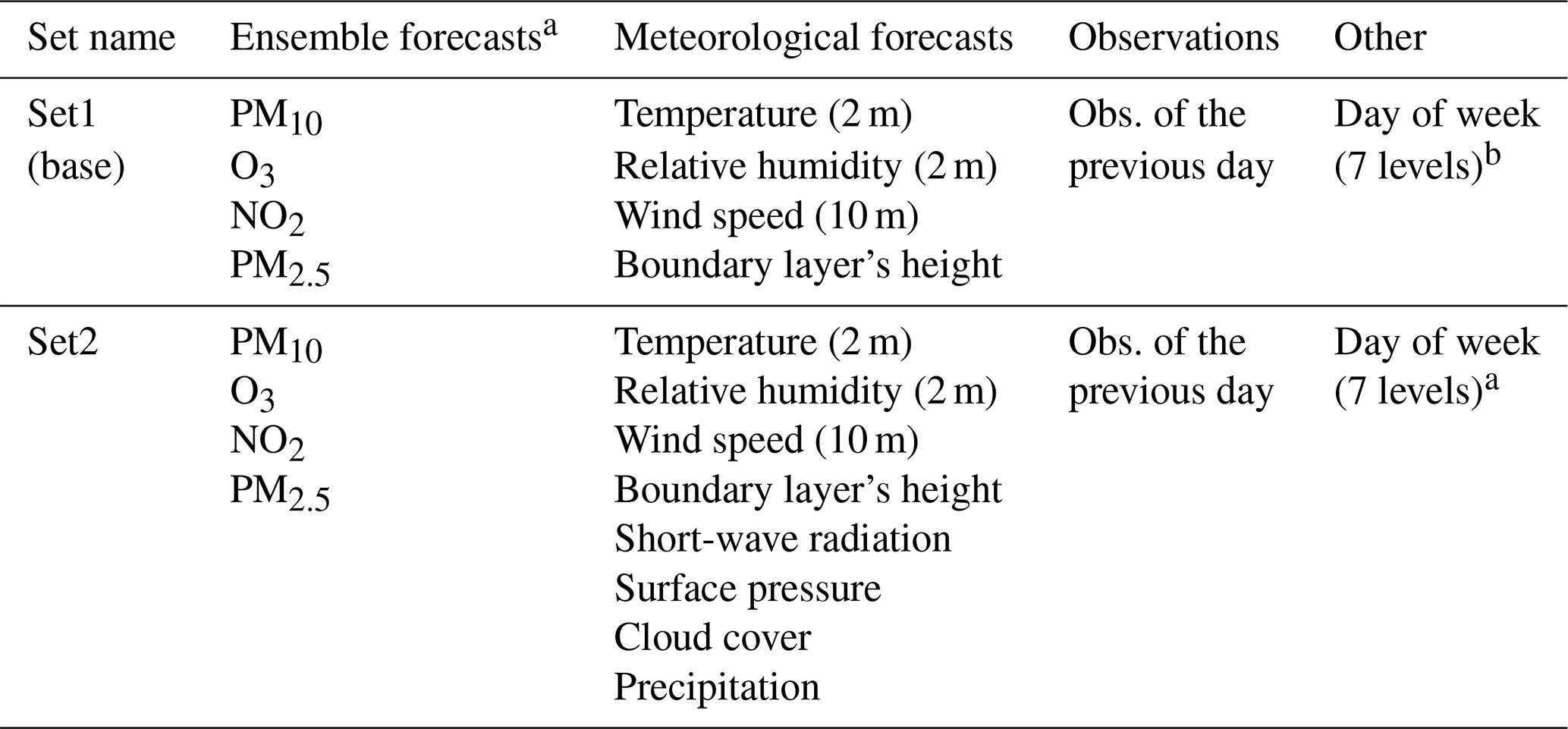
a Raw or unbiased (for the global approach only) concentration forecasts. b Only for the local (or long training) approach.
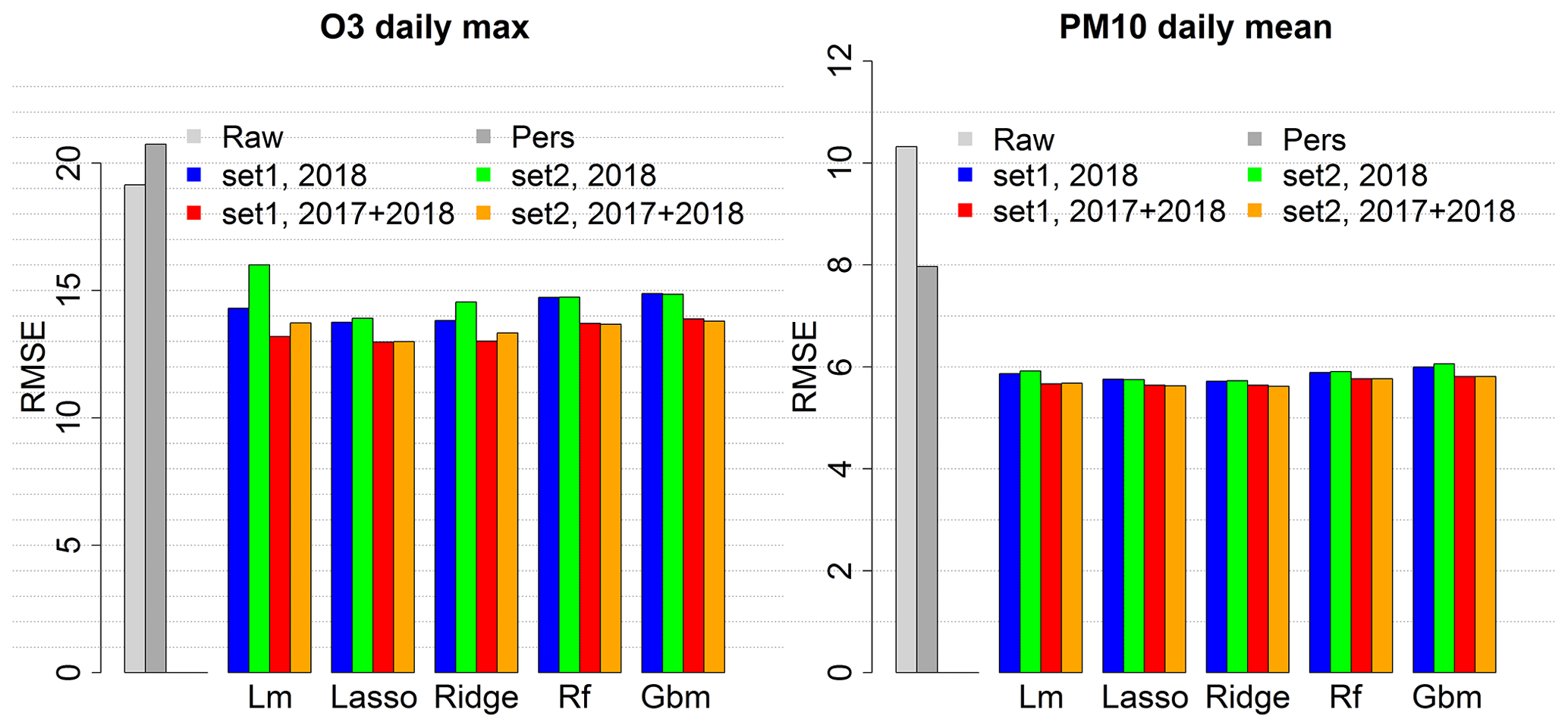
Figure 1RMSE score for the raw ensemble (Raw) and local MOS approaches with the linear model (Lm), the LASSO (Lasso), the ridge (Ridge), the random forest (Rf) and the gradient boosting model (Gbm), depending on the training period and set of predictors. RMSE score is averaged over 1535 stations for O3 and 957 stations for PM10. Evaluation was done over 2019 summer months for ozone and whole the year 2019 for PM10.
Specific local approach simulations have been carried out to evaluate O3 daily max and PM10 daily mean predictions performances with various input data configurations. Only O3 daily max and PM10 daily mean predictions have been considered in this preliminary analysis in order to limit the number of simulations. These forecasts are critical in Europe because of the frequent exceedances of the regulatory threshold values that determine pollution peaks (180 µg m−3 for O3 daily max and 50 µg m−3 for PM10 daily mean). Each pollutant was tested with two configurations regarding the size of the training dataset. For O3, one summer (June–September 2018) or two summers (June–September 2017 and 2018) have been used as training datasets. For PM10, year-round data have been used, either 1 year (2018) or 2 years (2017 and 2018). A training period limited to summer months has been chosen for O3 to optimize the performances during this season which is regularly subject to critical concentration levels. Similarly, the model could be optimized for the cold season using winter months for training, and year-round modelling could be achieved by switching from one model to the other at some point during the inter-season. But we chose to limit our analysis to the hot season when most pollution peaks happen. In addition, both configurations have been tested using two distinct sets of predictors, namely Set1, the simplest (includes the base predictors plus the categorical day of week predictor), and Set2, including four additional meteorological predictors (see Table 1). Performances have been evaluated with 2019 data, over the summer season (June–September) for O3 and the whole year for PM10. As expected, the RMSE of the local MOS score average over all the monitoring stations, shown in Fig. 1, is significantly reduced in comparison to that of the raw ensemble model. The MOS allows us to greatly reduce the bias (see also Fig. B1) and thus to significantly decrease the RMSE. The use of larger datasets is beneficial for all the machine learning algorithms tested and is particularly interesting for O3 daily max predictions (RMSE strongly decreases when using 8 months of summer data instead of 4). Results also suggest being very careful with the choice of predictors, using more predictors as in Set2 generally leads to no improvement or even a loss in performance, especially if the algorithm is not designed to handle overfitting and if the training period is too short (see the deterioration of the O3 RMSE when using the larger set of predictors, Set2, in the standard linear model). In addition to the raw ensemble and the five MOS values, the persistence model (Pers), a very simple reference model which consists of forecasting for the day ahead the concentration that was observed at the station during the previous day, is plotted for comparison. Whatever the configuration, the MOS models allow us to beat the RMSE score of this persistence model. Regularized linear models (ridge and LASSO) give the best RMSE scores independently of the set of predictors and of the size of the training period. With 2017 and 2018 data for training and the simplest set of predictors (red bar), the RMSE reaches 13.0 µg m−3 for O3 daily max (decrease of 32 % compared to the raw ensemble) and 5.64 µg m−3 for PM10 daily mean (decrease of 45 %). The Pearson correlation reaches 0.86 for O3 (against 0.81 for the raw ensemble) and 0.83 for PM10 (against 0.7 for the raw ensemble). See Figs. B1 and B2 for the mean bias and correlation scores with the distinct local approach modelling configurations.
For the global approach, tests have been performed over the same 2019 periods (summer for O3 and whole year for PM10) with the simplest set of predictors, Set1, to evaluate O3 daily max and PM10 daily mean MOS prediction according to the size of the training period (3, 7 and 14 d) and the use of the raw (biased) or unbiased concentration forecasts as predictor. Figure 2 illustrates the decrease in RMSE when using unbiased concentrations instead of raw concentrations (compare the blue and plain green bars for 3 d training). RMSE can further be improved using 7 d as training period or even 14 d for PM10 daily mean. The random forest model gives the best RMSE scores independently of the length of the training period. With 14 d for training and using the unbiased concentration predictor, the RMSE reaches 12.5 µg m−3 for O3 daily max (decrease of 34.6 % compared to the raw ensemble) and 5.5 µg m−3 for PM10 daily mean (decrease of 46.7 %). The Pearson correlation reaches 0.85 for O3 (against 0.81 for the raw ensemble) and 0.83 for PM10 (against 0.7 for the raw ensemble). See Figs. B3 and B4 for the mean bias and correlation scores with the distinct global approach modelling configurations.
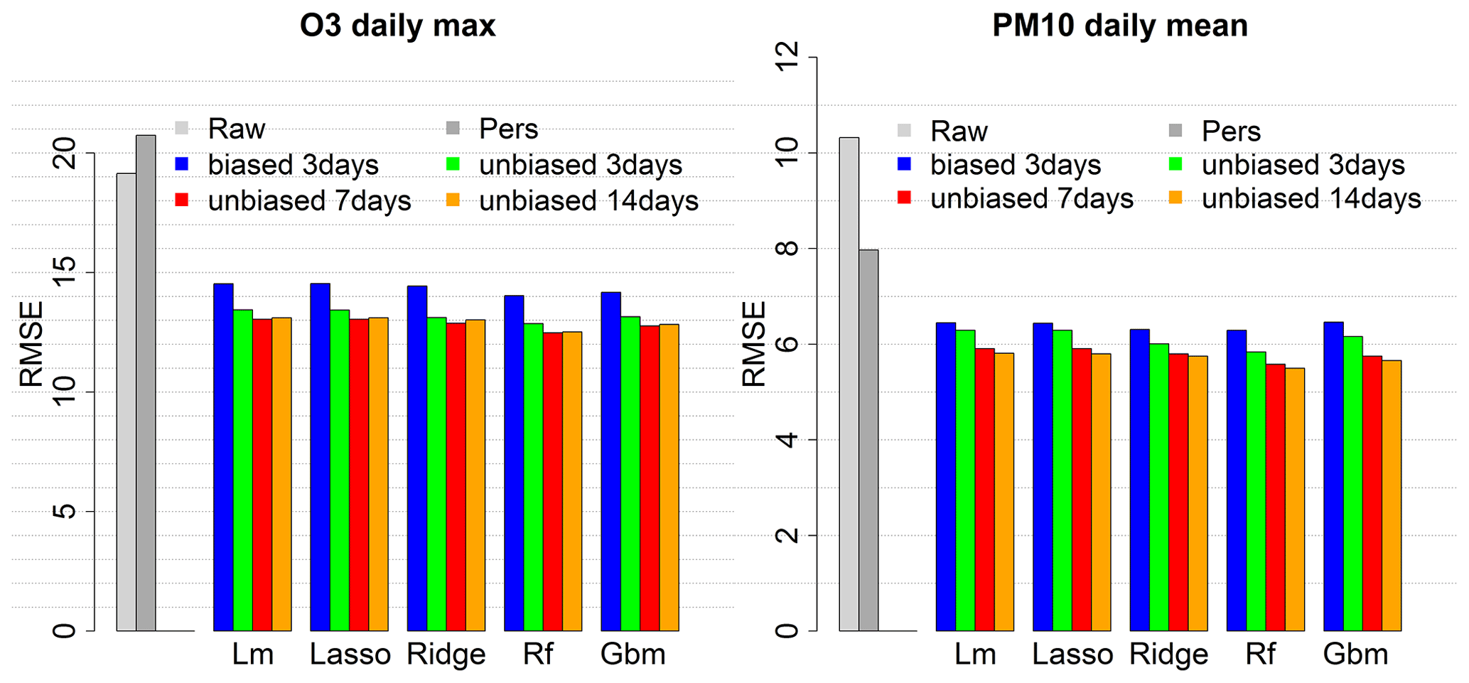
Figure 2RMSE score for the raw ensemble (Raw) and global MOS approaches with the linear model (Lm), the LASSO (Lasso), the ridge (Ridge), the random forest (Rf) and the gradient boosting model (Gbm), depending on the training period and the use of biased or unbiased concentration predictors. RMSE score is averaged over 1535 stations for O3 and 957 stations for PM10. Evaluation was done over 2019 summer months for ozone and the whole year 2019 for PM10.
For the four pollutants, O3, PM10, NO2 and PM2.5, the local and global MOS have been designed for the prediction of daily mean, daily max and hourly concentrations and compared to each other. For both the local and global approaches, since the benefit of using four additional predictors in Set2 compared to Set1 was not confirmed in Sect. 4, we used the simplest sets of predictors (Set1, with unbiased concentrations for the global approach). Moreover, we used in this section the more realistic scenario where only 1 full year of data (2018) is available for training the local approach models. For the global approach, we present the 3 d training scenario which is supposed to adapt faster to a change in the modelling system. As mentioned above, performances can be optimized using larger training periods, but we chose to test the scenario which is more prone to cope with operational constraints. Table 2 shows RMSE scores averaged over the full set of monitoring stations across Europe with the 2019 testing period. As in the previous section, evaluation is focused on the June–September period for O3 and whole year for PM10, PM2.5 and NO2.
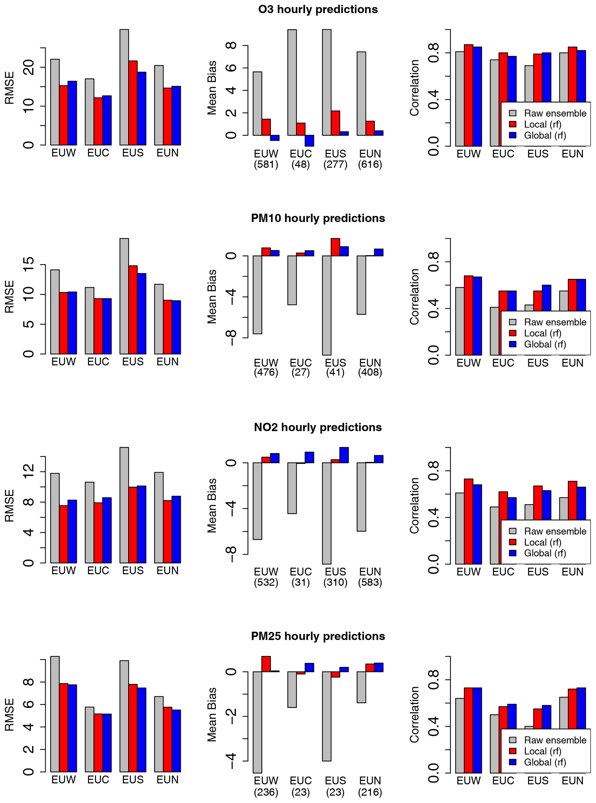
Figure 3Comparison of the raw ensemble model and best model scenarios for the local and global MOS approaches. Scores include station means of RMSE, mean bias and correlation for the prediction of hourly mean concentrations over central Europe (EUC), northern Europe (EUN), southern Europe (EUS) and western Europe (EUW).
Table 2The 2019 RMSE score (average of 1535 (O3), 957 (PM10), 1468 (NO2) and 498 (PM2.5) stations) for daily mean, daily maximum and hourly mean as percentage of decrease compared to the raw model RMSE. Raw model RMSE (in µg m−3) is indicated in the “Raw” column.
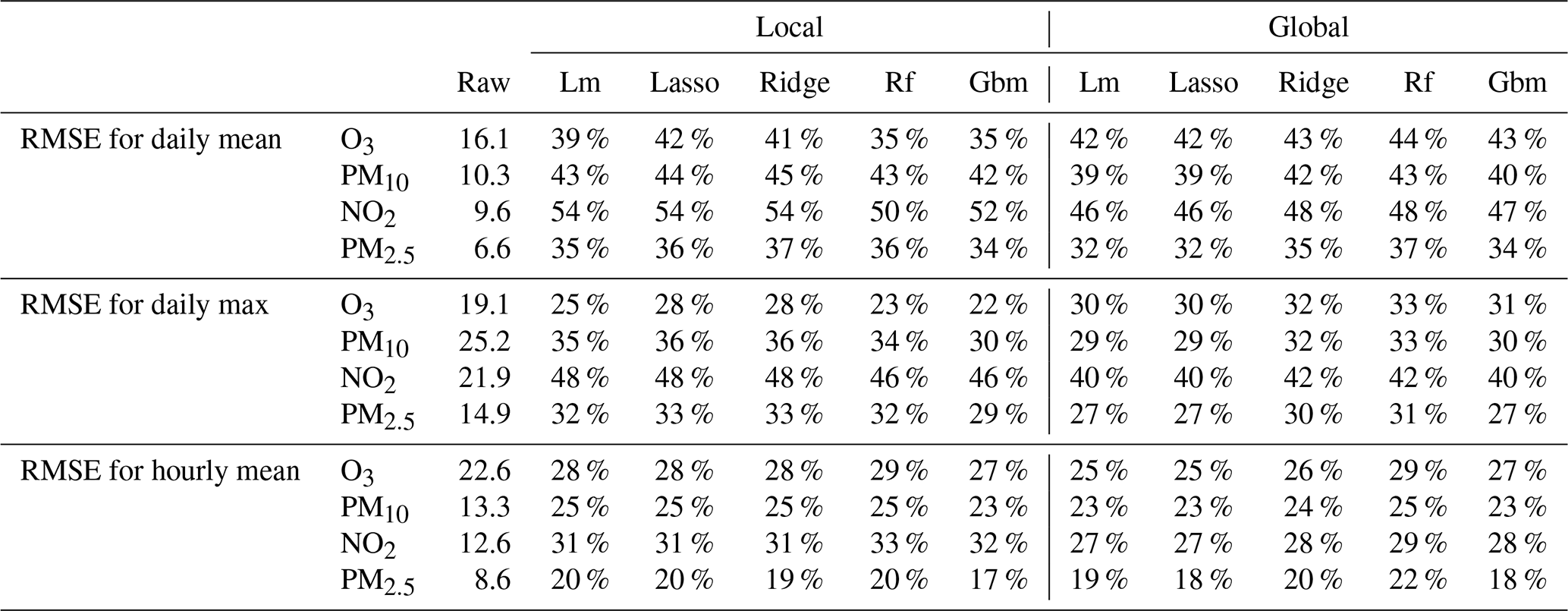
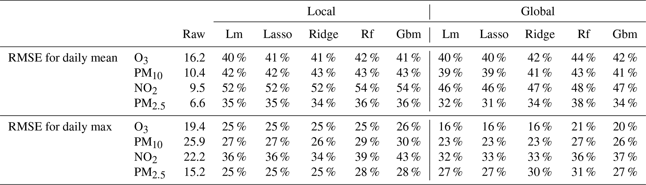
The random forest is particularly adapted to optimize the RMSE of the global MOS approach as the best scores are obtained with this model for the four pollutants and for the predictions of daily mean, daily max and hourly concentrations. Depending on the prediction objective and on the pollutant, the improvement compared to the raw ensemble oscillates between 48.1 % (decrease in RMSE) and 21.9 %. The choice of the best algorithm is not that clear for the local MOS approach. Random forest gives the best RMSE for the prediction of hourly means, but the LASSO and ridge linear models perform the best for daily means and daily max predictions. RMSE decreases oscillate between 54.1 % (NO2 daily max) and 20 % (PM2.5 hourly mean) with the best model scenarios for this local approach. Still considering the best model scenarios, differences between the local and global approach reach 6.3 %, in favour of the local approach, for NO2 daily max predictions and 4.6 %, in favour of the global approach, for O3 daily max predictions. Table 3 presents the RMSE scores for the daily mean and daily max extracted from hourly MOS predictions. These scores are comparable with those of the models specifically trained for daily mean predictions but are significantly degraded for daily max predictions. As an example, the global approach with random forest model reduces the RMSE by 20.5 % when daily max values are extracted from hourly predictions, against a reduction of 32.8 % with the same model trained for daily max prediction. Therefore, depending on applications, one might consider using daily MOS instead of hourly MOS if performances must be optimized for the daily max statistics.
Table 3The 2019 RMSE scores as percentage of decrease compared to the raw ensemble model for the daily mean and daily max extracted from the hourly MOS predictions.
For the four pollutants investigated in this study, this reduction in RMSE score is associated with a strong decrease in the mean bias. As illustrated in Fig. 3 for the prediction of hourly concentrations, the raw ensemble model tends to overestimate O3 levels and to underestimate PM10, PM2.5 and NO2 concentrations in central Europe (EUC), northern Europe (EUN), southern Europe (EUS) and western Europe (EUW). These biases are well corrected by both the local and global MOS (see the red and blue bars which represent the local and global MOS approaches with their respective best model scenarios). The reduction in RMSE is also associated with a significant increase in the correlation score. Similar results have been obtained with the MOS designed for daily mean and daily max (see Appendix C). While the local and global approaches compete with each other for O3, PM10, and PM2.5 daily and hourly forecasts, the local approach outperforms the global approach for the NO2 pollutant. This difference is attributed to the local nature of this pollutant, i.e. the fact that concentration levels are more influenced by local emission, and to a smaller extent by meteorological conditions. However, the global MOS approach still clearly improves performances compared to the raw ensemble model for this pollutant.
The European Union has defined concentration thresholds to characterize pollution peaks. Exceedance of these thresholds requires authorities to inform the exposed population and the set-up of mitigation actions by local authorities to reduce the adverse effects of the pollution. We therefore paid special attention to the ability of the models to detect such threshold exceedances. The threshold value of 180 µg m−3 for O3 daily max concentration and 50 µg m−3 for PM10 daily mean are regularly exceeded in Europe. These exceedances events remain relatively rare. In our 2019 testing dataset (only summer months for O3), the base rate is 1.3 % and 2 %, respectively, for O3 and PM10 exceedances. On average, the duration of these episodes of exceedances at a station is 1.6 d for O3, with 30 % of the episodes lasting 2 d or more and 4 % lasting 5 d or more. For PM10, the episodes tend to be a little bit longer, with an average duration of 1.8 d, with 40 % of the episodes lasting 2 d or more and 5 % lasting 5 d or more.
To assess the ability of a model to detect these exceedances, we use the so-called contingency table which counts the number of good detections (predicted and observed exceedances), missed (observed but not predicted) and false alarms (predicted but not observed) over the whole set of monitoring stations. Figure 4 represents the contingency table for O3 daily max exceedances and PM10 daily mean exceedances of the raw ensemble model and the local MOS. The persistence model, referred to as “Pers”, has been added to the plot as a reference. It is a trivial model which consists of forecasting for the next day the concentration that we observed during the previous day. To characterize detection skills, four scores can be derived from the contingency table and plotted into a single performance diagram (Figs. 5 and 6). The probability of detection (on the y axis) is defined as the ratio of good detections to the total number of observed exceedances, the success ratio (x axis) is defined as the ratio of good detections to the total number of predicted exceedances, the critical success index (CSI) represented by the black contours is the ratio of good detections to the total number of predicted or observed exceedances, and the frequency bias (dashed straight line) is the ratio of the total number of predicted exceedances to the total number of observed exceedances. All these scores take values between 0 and 1, except for the frequency bias which takes any positive value. A perfect model would take the value of 1 for all these scores and would be located in the upper right corner of the performance diagram.
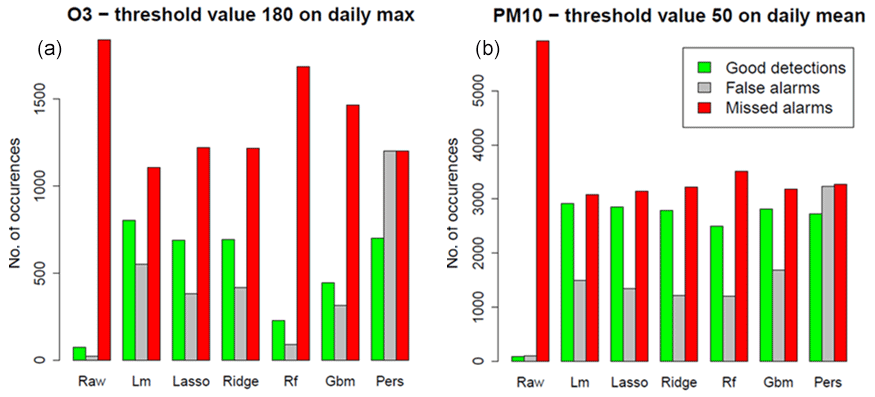
Figure 4Contingency table of the raw ensemble, the local MOS models and the persistence model, over the 2019 testing period, for O3 (a) and PM10 (b) threshold exceedances.
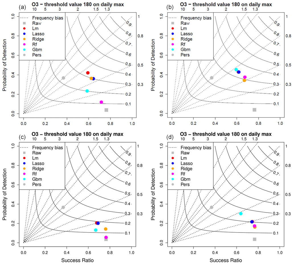
Figure 5Detection scores for the local daily (a), global daily (b), local hourly (c) and global hourly (d) MOS approaches for O3 daily max 180 µg m−3 threshold.
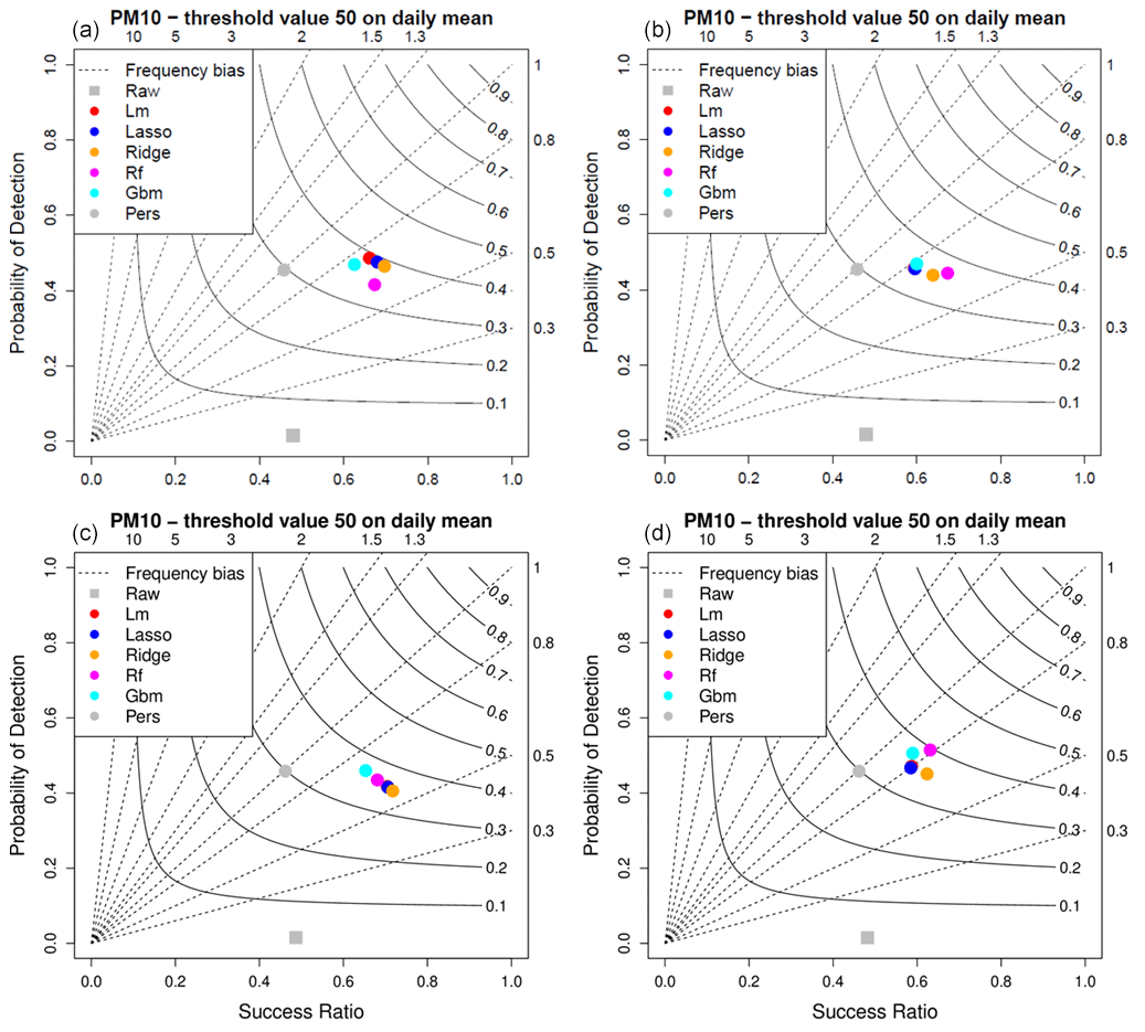
Figure 6Detection scores for the local daily (a), global daily (b), local hourly (c) and global hourly (d) MOS approaches for PM10 daily mean 50 µg m−3 threshold.
Figures 5 and 6 illustrate the detection performances of the MOS for O3 and PM10, respectively. In both figures, four performance diagrams represent the scores for the local daily (top left) and global daily (top right), as well as local hourly (bottom left) and global hourly (bottom right) MOS approaches. For O3 (Fig. 5), the high value (close to 0.8) of the success ratio for the raw ensemble model means that when it detects a threshold exceedance there is a high probability to actually observe a threshold exceedance. But the downside is that observed exceedances have a very low probability to be detected by this model as illustrated by the very low probability of detection (y axis). In other words, the raw model is strongly biased (in frequency) with much more observed than predicted exceedances. In contrast, the MOS allows us to get a frequency bias closer to 1, reducing the success ratio but greatly improving the probability of detection. Both the local and global approaches enable us to improve the overall detection performances, reaching CSI scores between 0.3 and 0.4 for the MOS dedicated to daily predictions (see the top panels). The small loss in the success ratio is largely compensated by the gain in probability of detection. In that configuration, with 4 months of data for training, the local approach works better with linear models (standard, LASSO and ridge) than with tree-based models (RF and GBM). The best CSI score is obtained with the global-daily approach and GBM model (0.34). This is much better than the persistence model which produces a CSI score of 0.22. Note that, by construction, the frequency bias of the persistence model (grey circle in the performance diagrams) is equal to one (i.e. located over the bisector of the performance diagram) since the number of predicted exceedances always equals the number of observed exceedances (exceedances are predicted with 1 d of delay). The position on the bisector line depends on the length of the episodes. Long episodes of exceedances (several consecutive days) will tend to produce good scores (closer to the upper right corner of the performance diagram). For this O3 threshold of exceedance, performances are clearly degraded when using the hourly approach (bottom panels).
Results are comparable for the detection of exceedances of PM10 daily mean threshold (Fig. 6), with success ratio scores between 0.59 and 0.68, probability of detection between 0.42 and 0.51, and CSI between 0.35 and 0.4 depending on the MOS approach and on the model considered. The best CSI score of 0.4 is obtained with the global-hourly approach associated with the random forest model. Unlike the O3 pollutant, detection performances of the hourly approaches are similar to those of the daily approaches.
This work allows us to compare the performances of two model output statistics (MOS) approaches for the correction of the Copernicus Atmosphere Monitoring Service (CAMS) forecasts for four regulated pollutants for the upcoming day at daily and hourly timescales, at monitoring sites covering the European territory. Both approaches (local and global) are implemented with five distinct machine learning algorithms ranging from simple linear regressions to more sophisticated tree-based models. The construction of optimized local MOS needs relatively long periods of data available for training individual models at each site. It was therefore tested with a reasonable scenario, where a full year of training data was available for PM10, PM2.5 and NO2 pollutants. For O3, we focused on summer predictions, and the MOS was trained with 4 months of summer data. In this context, the local MOS approach performs best with the linear models for the RMSE of daily predictions and for detection performances, while the random forest model gives the best RMSE scores for the hourly predictions. We insist that this result is only true with 1 year (four summer months for O3) of training data. It could be different with a shorter training period as linear models are more prone to overfitting as suggested by the results described in Sect. 4. The global MOS is an innovative approach designed to cope with operational constraints. Its very short training period (3 d) allows us to adapt in a short time to any changes in the modelling system (upgrade of the deterministic model, addition of new monitoring stations). In addition to its operational flexibility, the global approach shows performances that compete with those of the local approach. For this global approach, the random forest algorithm gives the best RMSE scores whatever the pollutant and timescale considered. However, if the MOS is designed for hourly prediction, the gradient boosting machine (GBM) algorithm is more adapted than random forest to detect O3 daily max threshold exceedances. We would therefore recommend the GBM model in that situation. But one might also consider using a MOS specifically designed for daily maximum predictions to further improve detection skills.
As mentioned above, the local approach was performed in this study with a relatively large training dataset. Interestingly, such a local approach was tested with CAMS O3 forecasts by Petetin et al. (2022) using a selection of MOS methods (including basic methods such as persistence or moving average to more sophisticated methods such as GBM) to build a model at every monitoring station located in the Iberian Peninsula. To compare the distinct MOS methods, Petetin et al. (2022) mimic a worst-case operational scenario where very few prior data are available for training; that is, new models are trained regularly with a growing history, starting with 30 d and ending with 2 years of data for a February 2018–December 2019 simulation. Performances cannot be directly compared to this work because of their distinct spatial and temporal (year-round versus summer months) coverage. Nevertheless, the authors highlight that the GBM model presents poor detection skills (worse than the persistence model) despite having the best RMSE and correlation performances. Our study confirms this result for the GBM and random forest models, even with four summer months for training. We further demonstrate that with a constant 3 d training period, the global approach offers stable performances, with optimized continuous and categorical skills, from the very first days following a deterministic modelling system upgrade. As mentioned in Sect. 2, the CAMS ensemble model was subject to an upgrade in June 2019 (i.e. during the testing period). We verified that no breakup in the scores occurred during this period and thus consider that this upgrade had little impact on the local MOS (despite being calibrated with a slightly different CAMS ensemble version). Nevertheless, we emphasize that there is no reason that the local MOS will behave the same way in future upgrades and reaffirm the benefit of the global (short training) MOS approach to deal with those situations. In the future, such a global approach could also be used with a gradually expanding training dataset as in Petetin et al. (2022), being mindful, however, of the computing demand of automated learning of such a MOS in an operational set-up. Because of its flexibility, we also expect that this global approach is prone to adapt in real time to rapid changes in pollutant emissions as experimented with during the COVID crisis. Further investigation could be made using 2020 data to test this approach in such a situation.
For both the LASSO and ridge models, the penalty coefficient (lambda) is tested with values in {0, 0.05, [0.1 to 5.0 by increments of 0.1], 6, 7, 8, 10, 12, 15}. For the random forest algorithm, the number of trees (ntree) to grow is fixed to 100, and the number of variables randomly sampled at each split (mtry) is taken as the largest integer less than or equal to the square root of P, where P is the number of predictors. For the GBM algorithm, the number of trees (n.tree) is fixed to 100. The learning rate (shrinkage) takes values in . The number of splits to perform in each tree (interaction.depth) takes values in {2,7}, and the minimum number of observations in a node (n.minobsinnode) takes values in {1,5}.
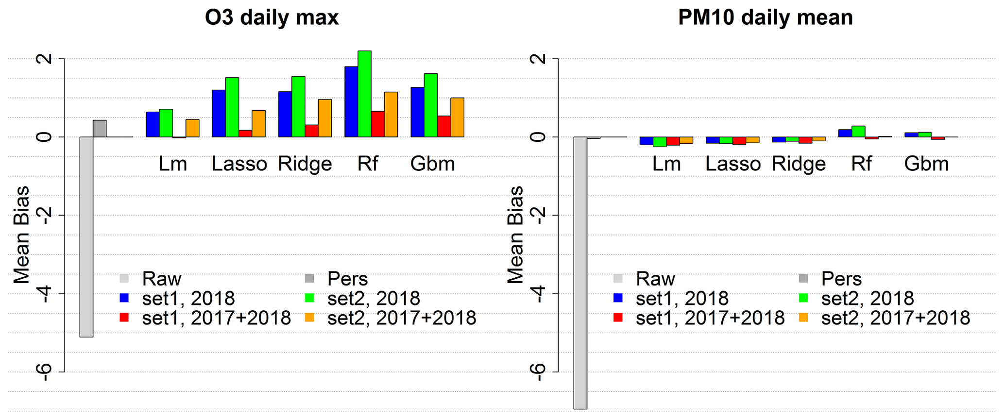
Figure B1Mean bias score for the raw ensemble model and the local MOS approach with four training configurations.
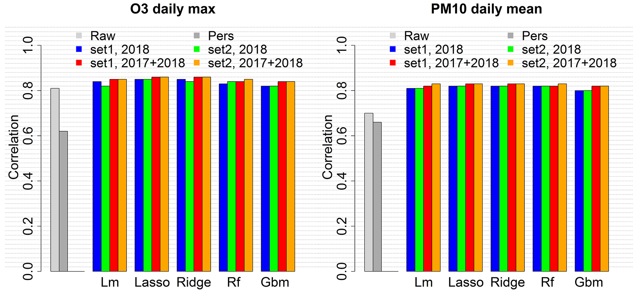
Figure B2Correlation score for the raw ensemble model and the local MOS approach with four training configurations.
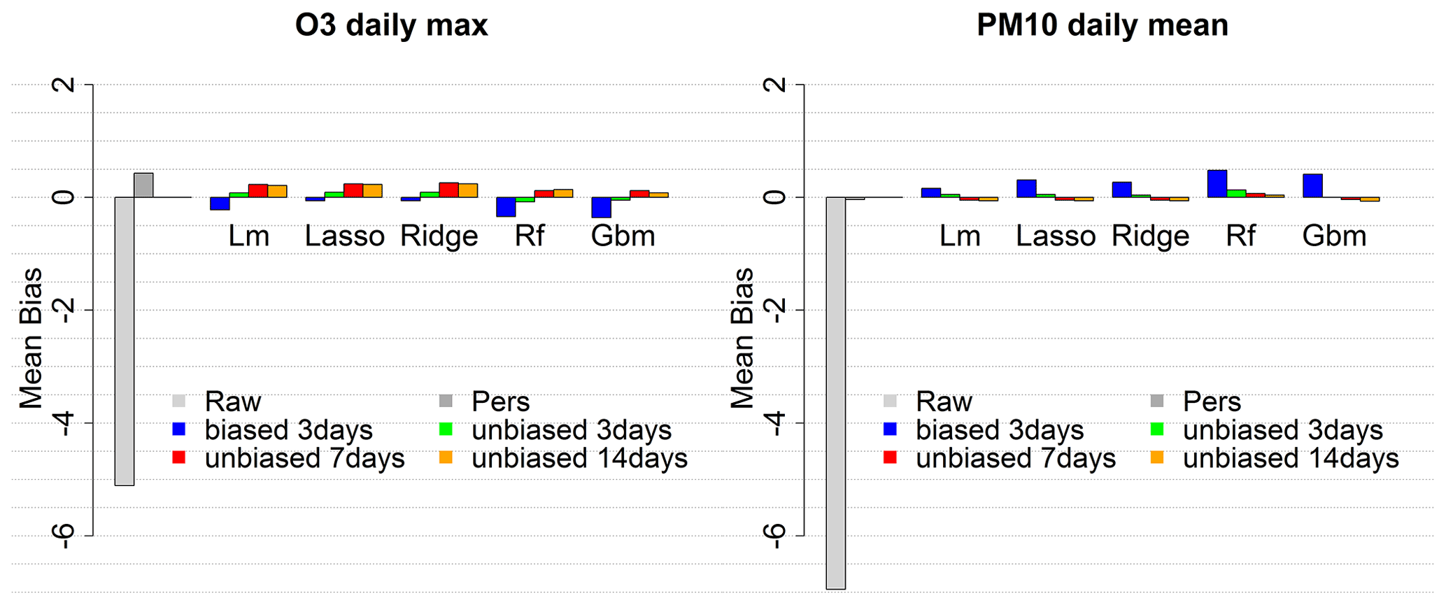
Figure B3Mean bias score for the raw ensemble model and the global MOS approach with four training configurations.
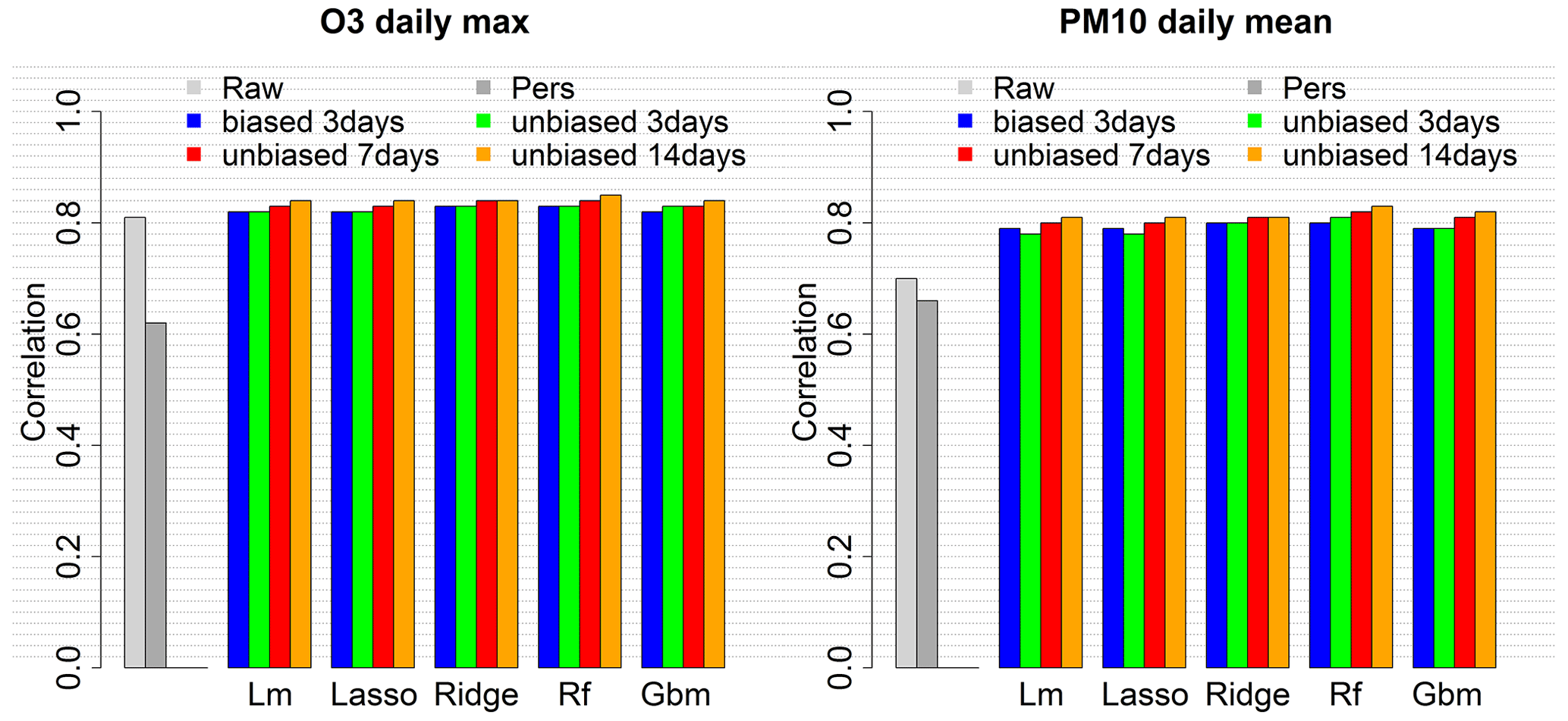
Figure B4Correlation score for the raw ensemble model and the global MOS approach with four training configurations.
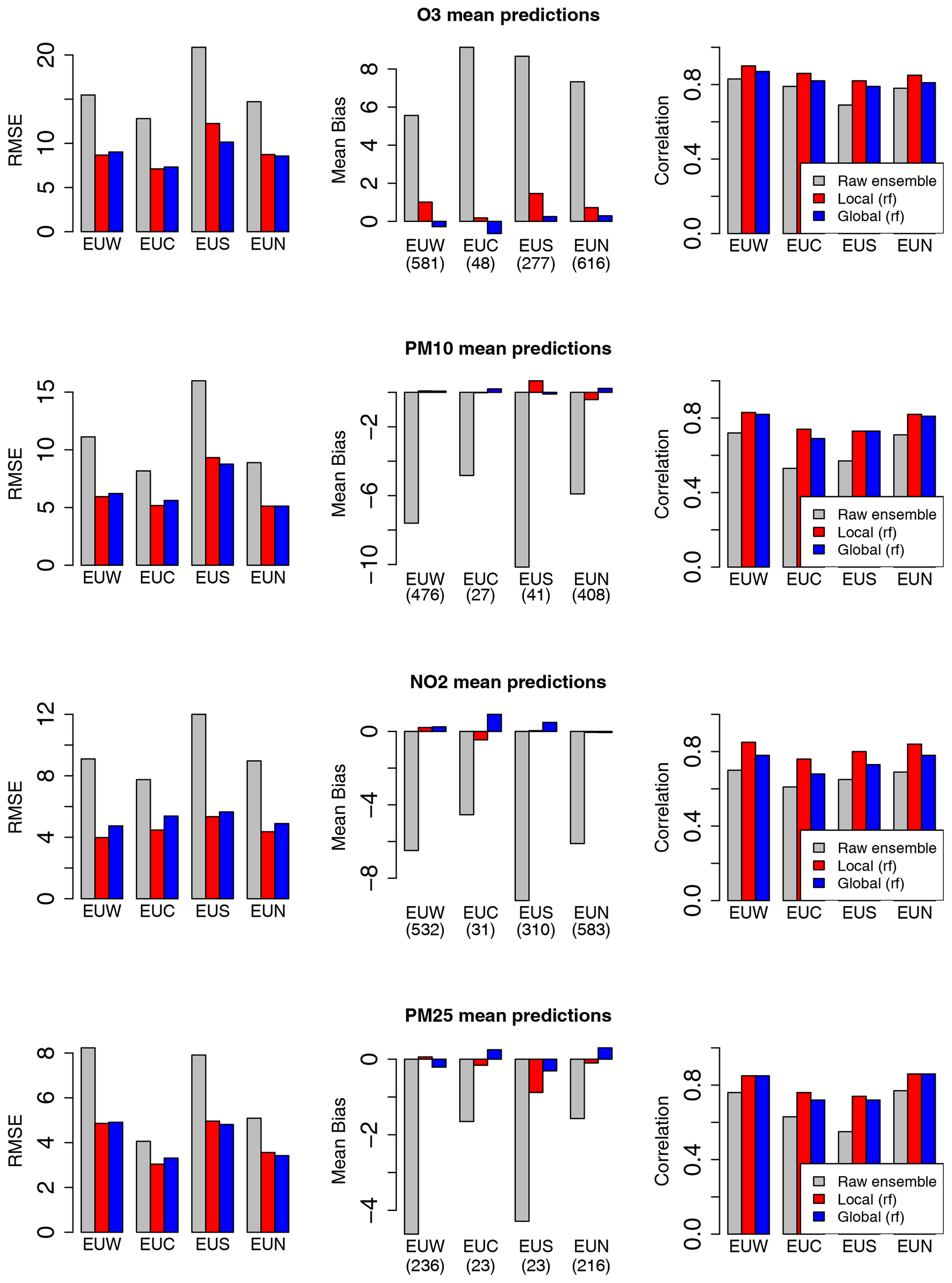
Figure C1Comparison of the raw ensemble model and best model scenarios for the local and global MOS approaches. Scores include station means of RMSE, mean bias and correlation for the prediction of daily mean concentrations over central Europe (EUC), northern Europe (EUN), southern Europe (EUS) and western Europe (EUW).
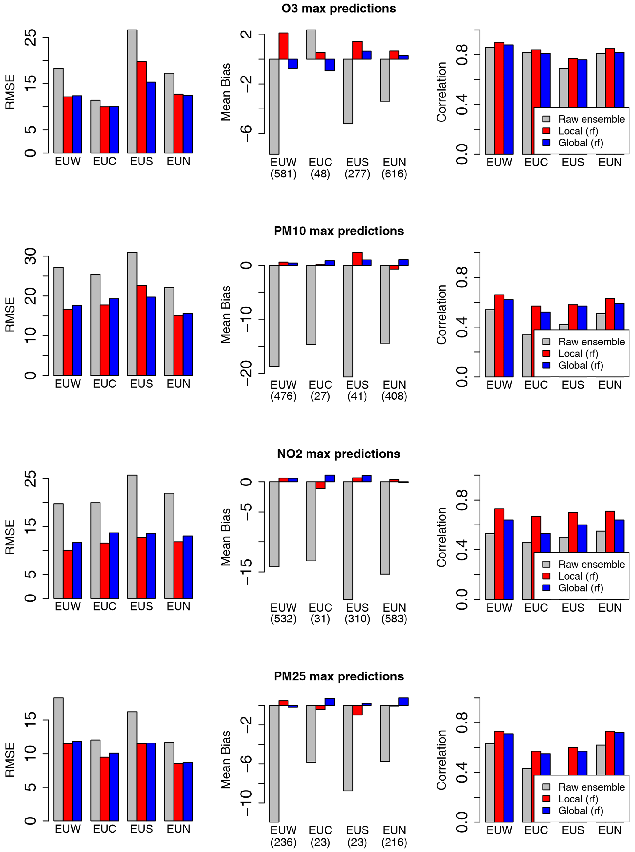
Figure C2Comparison of the raw ensemble model and best model scenarios for the local and global MOS approaches. Scores include station means of RMSE, mean bias and correlation for the prediction of daily max concentrations over central Europe (EUC), northern Europe (EUN), southern Europe (EUS) and western Europe (EUW).
The modelling results used in the present study are archived by the authors and can be obtained from the corresponding author upon request.
JMB worked on the implementation of the study and performed the simulations with support from all the co-authors. AU was responsible for the acquisition of the observed air quality data. JMB performed the analysis with the support of GD, AU, FM and AC for results interpretation. JMB wrote this article, with contributions from FM and AC.
The contact author has declared that none of the authors has any competing interests.
Publisher's note: Copernicus Publications remains neutral with regard to jurisdictional claims in published maps and institutional affiliations.
The development of this work has received support from the Copernicus Atmosphere Monitoring Service of the European Union, implemented by ECMWF under service contracts CAMS_63 and CAMS2_40 and from the French Ministry in charge of ecology.
This research has been supported by the European Centre for Medium-Range Weather Forecasts (grant no. CAMS_63 and CAMS2_40) and by the French Ministry in charge of ecology.
This paper was edited by Stefano Galmarini and reviewed by two anonymous referees.
Badia, A. and Jorba, O.: Gas-phase evaluation of the online NMMB/BSC-CTM model over Europe for 2010 in the framework of the AQMEII-Phase2 project, Atmos. Environ., 115, 657–669, https://doi.org/10.1016/j.atmosenv.2014.05.055, 2015.
Breiman, L.: Random Forests, Mach. Learn., 45, 5–32, 2001.
Breiman, L., Friedman, J. H., Ohlsen, R. A., and Stone C. J.: Classification and Regression Trees, Chapman and Hall/CRC, ISBN 13:978-0412048418, 1984.
Christensen, J. H.: The Danish Eulerian hemispheric model – A three-dimensional air pollution model used for the Arctic, Atmos. Environ., 31, 4169–4191, 1997.
Delle Monache, L. and Stull, R. B.: An ensemble air quality forecast over western Europe during an ozone episode, Atmos. Environ., 37, 3469–3474, 2003.
Delle Monache, L., Nipen, T., Deng, X., Zhou, Y., and Stull, R.: Ozone ensemble forecasts: 2. A Kalman filter predictor bias correction, J. Geophys. Res., 111, D05308, https://doi.org/10.1029/2005JD006311, 2006.
Djalalova, I., Delle Monache, L., and Wilczak, J.: PM2.5 analog forecast and Kalman filter post-processing for the Community Multiscale Air Quality (CMAQ) model, Atmos. Environ., 108, 76–87, 2015.
Freund, Y. and Schapire, R.: Experiments with a new boosting algorithm, Machine Learning, in: Proceedings of the Thirteenth International Conference, Morgan Kauffman, San Francisco, 148–156, ISBN 10:1-55860-419-7, 1996.
Friedman, J., Hastie, T., and Tibshirani, R.: Regularization Paths for Generalized Linear Models via Coordinate Descent, J. Stat. Softw., 33, 1–22, 2010.
Friedman, J. H.: Greedy Function Approximation: a Gradient Boosting Machine, Ann. Stat., 29, 1189–1232, https://doi.org/10.1214/aos/1013203451, 2001.
Grange, S. K., Carslaw, D. C., Lewis, A. C., Boleti, E., and Hueglin, C.: Random forest meteorological normalisation models for Swiss PM10 trend analysis, Atmos. Chem. Phys., 18, 6223–6239, https://doi.org/10.5194/acp-18-6223-2018, 2018.
Greenwell, B., Boehmke, B., Cunningham, J., and GBM Developers: Generalized Boosted Regression Models, r package version 2.1.5, http://CRAN.R-project.org/package=gbm (last access: 13 April 2023), 2019.
Guth, J., Josse, B., Marécal, V., Joly, M., and Hamer, P.: First implementation of secondary inorganic aerosols in the MOCAGE version R2.15.0 chemistry transport model, Geosci. Model Dev., 9, 137–160, https://doi.org/10.5194/gmd-9-137-2016, 2016.
Hass, H., Jakobs, H. J., and Memmesheimer, M.: Analysis of a regional model (EURAD) near surface gas concentration predictions using observations from networks, Meteorol. Atmos. Phys., 57, 173–200, https://doi.org/10.1007/BF01044160, 1995.
Hoerl, A. and Kennard, R.: Ridge Regression: Biased Estimation for Nonorthogonal Problems, Technometrics, 12, 55–67, https://doi.org/10.1080/00401706.1970.10488634, 1970.
Honoré, C., Rouïl, L., Vautard, R., Beeckmann, M., Bessagnet, B., Dufour, A., Elichegaray, C., Flaud, J.-M., Malherbe, L., Meleux, F., Menut, L., Martin, D., Peuch, A., Peuch, V.-H., and Poisson, N.: Predictability of European air quality: Assessment of 3 years of operational forecasts and analyses by the PREV'AIR system, J. Geophys. Res., 113, D04301, https://doi.org/10.1029/2007JD008761, 2008.
Kaminski, J. W., Neary, L., Struzewska, J., McConnell, J. C., Lupu, A., Jarosz, J., Toyota, K., Gong, S. L., Côté, J., Liu, X., Chance, K., and Richter, A.: GEM-AQ, an on-line global multiscale chemical weather modelling system: model description and evaluation of gas phase chemistry processes, Atmos. Chem. Phys., 8, 3255–3281, https://doi.org/10.5194/acp-8-3255-2008, 2008.
Kang, D., Mathur, R., Rao, S. T., and Yu, S.: Bias adjustment techniques for improving ozone air quality forecasts, J. Geophys. Res., 113, D23308, https://doi.org/10.1029/2008JD010151, 2008.
Kuhn, M.: Building predictive models in R using the caret package, J. Stat. Softw., 28, 1–26, https://doi.org/10.18637/jss.v028.i05, 2008.
Liaw, A. and Wiener, M.: Classification and Regression by random forest, R News, 2, 18–22, 2002.
Mailler, S., Menut, L., Khvorostyanov, D., Valari, M., Couvidat, F., Siour, G., Turquety, S., Briant, R., Tuccella, P., Bessagnet, B., Colette, A., Létinois, L., Markakis, K., and Meleux, F.: CHIMERE-2017: from urban to hemispheric chemistry-transport modeling, Geosci. Model Dev., 10, 2397–2423, https://doi.org/10.5194/gmd-10-2397-2017, 2017.
Marécal, V., Peuch, V.-H., Andersson, C., Andersson, S., Arteta, J., Beekmann, M., Benedictow, A., Bergström, R., Bessagnet, B., Cansado, A., Chéroux, F., Colette, A., Coman, A., Curier, R. L., Denier van der Gon, H. A. C., Drouin, A., Elbern, H., Emili, E., Engelen, R. J., Eskes, H. J., Foret, G., Friese, E., Gauss, M., Giannaros, C., Guth, J., Joly, M., Jaumouillé, E., Josse, B., Kadygrov, N., Kaiser, J. W., Krajsek, K., Kuenen, J., Kumar, U., Liora, N., Lopez, E., Malherbe, L., Martinez, I., Melas, D., Meleux, F., Menut, L., Moinat, P., Morales, T., Parmentier, J., Piacentini, A., Plu, M., Poupkou, A., Queguiner, S., Robertson, L., Rouïl, L., Schaap, M., Segers, A., Sofiev, M., Tarasson, L., Thomas, M., Timmermans, R., Valdebenito, Á., van Velthoven, P., van Versendaal, R., Vira, J., and Ung, A.: A regional air quality forecasting system over Europe: the MACC-II daily ensemble production, Geosci. Model Dev., 8, 2777–2813, https://doi.org/10.5194/gmd-8-2777-2015, 2015.
Mircea, M., Ciancarella, L., Briganti, G., Calori, G., Cappelletti, A., Cionni, I., Costa, M., Cremona, G., D'Isidoro, M., Finardi, S., Pace, G., Piersanti, A., Righini, G., Silibello, C., Vitali, L. and Zanini, G.: Assessment of the AMS-MINNI system capabilities to simulate air quality over Italy for the calendar year 2005, Atmos. Environ., 84, 178–188, 2014.
Petetin, H., Bowdalo, D., Soret, A., Guevara, M., Jorba, O., Serradell, K., and Pérez García-Pando, C.: Meteorology-normalized impact of the COVID-19 lockdown upon NO2 pollution in Spain, Atmos. Chem. Phys., 20, 11119–11141, https://doi.org/10.5194/acp-20-11119-2020, 2020.
Petetin, H., Bowdalo, D., Bretonnière, P.-A., Guevara, M., Jorba, O., Mateu Armengol, J., Samso Cabre, M., Serradell, K., Soret, A., and Pérez Garcia-Pando, C.: Model output statistics (MOS) applied to Copernicus Atmospheric Monitoring Service (CAMS) O3 forecasts: trade-offs between continuous and categorical skill scores, Atmos. Chem. Phys., 22, 11603–11630, https://doi.org/10.5194/acp-22-11603-2022, 2022.
Robertson, L., Langner, J., and Engardt, M.: An Eulerian limited-area atmospheric transport model, J. Appl. Meteorol. Clim., 38, 190–210, 1999.
Rouïl, L., Honoré, C., Vautard, R., Beeckmann, M., Bessagnet, B., Malherbe, L., Meleux, F., Dufour, A., Elichegaray, C., Flaud, J.-M., Menut, L., Martin, D., Peuch, A., Peuch, V.-H., and Poisson, N.: PREV'AIR: An operational forecasting and mapping system for air quality in Europe, B. Am. Meteorol. Soc., 90, 73–84, https://doi.org/10.1175/2008BAMS2390.1, 2009.
Schaap, M., Manders, A. M. M., Hendriks, E. C. J., Cnossen, J. M., Segers, A. J. S., Denier van der Gon, H., Jozwicka, M., Sauter, F. J., Velders, G. J. M., Matthijsen, J., and Builtjes, P. J. H.: Regional Modelling of Particulate Matter for the Netherlands Netherlands Research Program on Particulate Matter, Report 500099008, PBL Netherlands Environmental Assesment Agency, ISSN 1875-2314, 2009.
Simpson, D., Benedictow, A., Berge, H., Bergström, R., Emberson, L. D., Fagerli, H., Flechard, C. R., Hayman, G. D., Gauss, M., Jonson, J. E., Jenkin, M. E., Nyíri, A., Richter, C., Semeena, V. S., Tsyro, S., Tuovinen, J.-P., Valdebenito, Á., and Wind, P.: The EMEP MSC-W chemical transport model – technical description, Atmos. Chem. Phys., 12, 7825–7865, https://doi.org/10.5194/acp-12-7825-2012, 2012.
Sofiev, M., Vira, J., Kouznetsov, R., Prank, M., Soares, J., and Genikhovich, E.: Construction of the SILAM Eulerian atmospheric dispersion model based on the advection algorithm of Michael Galperin, Geosci. Model Dev., 8, 3497–3522, https://doi.org/10.5194/gmd-8-3497-2015, 2015.
Tibshirani, R.: Regression shrinkage and selection via the lasso, J. Roy. Stat. Soc. B Met., 58, 267–288, 1996.
Wilczak, J., McKeen, S., Djalalova, I., Grell, G., Peckham, S., Gong, W., Bouchet, V., Moffet, R., McHenry, J., McQueen, J., Lee, P., Tang, Y., and Carmichael, G. R.: Bias-corrected ensemble and probabilistic forecasts of surface ozone over eastern North America during the summer of 2004, J. Geophys. Res.-Atmos., 111, D23S28, https://doi.org/10.1029/2006jd007598, 2006.
Zhang, Y., Bocquet, M., Mallet, V., Seigneur, C., and Baklanov, A.: Real-time air quality forecasting, Part I: History, techniques, and current status, Atmos. Environ., 60, 632–655, 2012.
Since then, four new models have been added to the ensemble calculation, namely DEHM (Christensen, 1997), GEMAQ (Kaminski et al., 2008), MINNI (Mircea et al., 2014) and MONARCH (Badia and Jorba, 2015).
https://www.ecmwf.int/en/research/modelling-and-prediction (last access: 13 April 2023).
- Abstract
- Introduction
- Training data
- Design of the MOS approaches
- Sensitivity of the MOS to training data and predictors
- Comparison of the local and global MOS approaches
- Conclusion
- Appendix A: Grids of tuning values for the hyper-parameters of each algorithm
- Appendix B
- Appendix C
- Data availability
- Author contributions
- Competing interests
- Disclaimer
- Acknowledgements
- Financial support
- Review statement
- References
globalapproach is proposed to drastically reduce the period necessary to train the models and thus facilitate the implementation in an operational context.
- Abstract
- Introduction
- Training data
- Design of the MOS approaches
- Sensitivity of the MOS to training data and predictors
- Comparison of the local and global MOS approaches
- Conclusion
- Appendix A: Grids of tuning values for the hyper-parameters of each algorithm
- Appendix B
- Appendix C
- Data availability
- Author contributions
- Competing interests
- Disclaimer
- Acknowledgements
- Financial support
- Review statement
- References