the Creative Commons Attribution 4.0 License.
the Creative Commons Attribution 4.0 License.
 | 24 Apr 2023
Evaluating Arctic clouds modelled with the Unified Model and Integrated Forecasting System
Gillian Young McCusker
Jutta Vüllers
Peggy Achtert
Paul Field
Jonathan J. Day
Richard Forbes
Ruth Price
Ewan O'Connor
Michael Tjernström
John Prytherch
Ryan Neely III
By synthesising remote-sensing measurements made in the central Arctic into a model-gridded Cloudnet cloud product, we evaluate how well the Met Office Unified Model (UM) and the European Centre for Medium-Range Weather Forecasting (ECMWF) Integrated Forecasting System (IFS) capture Arctic clouds and their associated interactions with the surface energy balance and the thermodynamic structure of the lower troposphere. This evaluation was conducted using a 4-week observation period from the Arctic Ocean 2018 expedition, where the transition from sea ice melting to freezing conditions was measured. Three different cloud schemes were tested within a nested limited-area model (LAM) configuration of the UM – two regionally operational single-moment schemes (UM_RA2M and UM_RA2T) and one novel double-moment scheme (UM_CASIM-100) – while one global simulation was conducted with the IFS, utilising its default cloud scheme (ECMWF_IFS).
Consistent weaknesses were identified across both models, with both the UM and IFS overestimating cloud occurrence below 3 km. This overestimation was also consistent across the three cloud configurations used within the UM framework, with >90 % mean cloud occurrence simulated between 0.15 and 1 km in all the model simulations. However, the cloud microphysical structure, on average, was modelled reasonably well in each simulation, with the cloud liquid water content (LWC) and ice water content (IWC) comparing well with observations over much of the vertical profile. The key microphysical discrepancy between the models and observations was in the LWC between 1 and 3 km, where most simulations (all except UM_RA2T) overestimated the observed LWC.
Despite this reasonable performance in cloud physical structure, both models failed to adequately capture cloud-free episodes: this consistency in cloud cover likely contributes to the ever-present near-surface temperature bias in every simulation. Both models also consistently exhibited temperature and moisture biases below 3 km, with particularly strong cold biases coinciding with the overabundant modelled cloud layers. These biases are likely due to too much cloud-top radiative cooling from these persistent modelled cloud layers and were consistent across the three UM configurations tested, despite differences in their parameterisations of cloud on a sub-grid scale. Alarmingly, our findings suggest that these biases in the regional model were inherited from the global model, driving a cause–effect relationship between the excessive low-altitude cloudiness and the coincident cold bias. Using representative cloud condensation nuclei concentrations in our double-moment UM configuration while improving cloud microphysical structure does little to alleviate these biases; therefore, no matter how comprehensive we make the cloud physics in the nested LAM configuration used here, its cloud and thermodynamic structure will continue to be overwhelmingly biased by the meteorological conditions of its driving model.
- Article
(15564 KB) - Full-text XML
-
Supplement
(3468 KB) - BibTeX
- EndNote


The Arctic is warming at more than twice the global average rate (Serreze and Barry, 2011; Cohen et al., 2014), with recent evidence suggesting the rate of warming could be up to 3 times the global average (AMAP, 2021). Coupled general circulation models (GCMs) fail to agree on the magnitude of recent warming and exhibit large biases in surface temperature and energy balance (Boeke and Taylor, 2016) driven largely by model parameter uncertainties on a decadal scale (Hodson et al., 2013). Biases in such surface properties are also present in atmosphere-only versions of these models with fixed ocean and sea ice boundaries, indicating that there is an important atmospheric source of disparity between models and reality (Bourassa et al., 2013). Arctic clouds have a net warming effect at the surface (Boucher et al., 2014) and are likely a contributing factor to the spread of surface energy balance estimates obtained from these models, with a large spread in cloud fractions, liquid water paths (LWPs), and ice water paths (IWPs) identified in past phases of the Coupled Model Intercomparison Project (CMIP; Karlsson and Svensson, 2011; Boeke and Taylor, 2016). Early results from the most recent CMIP indicate that high-latitude discrepancies in cloud fraction are still prevalent in recent revisions of these models (Vignesh et al., 2020).
With accelerating Arctic warming, we need to build suitable numerical models to confidently predict how the atmosphere will change on both short weather prediction scales and longer climate timescales (Jung et al., 2016). Models such as the Met Office Unified Model (UM) and the European Centre for Medium-Range Weather Forecasting (ECMWF) Integrated Forecasting System (IFS) are commonly used for assessing future Arctic change; however, recent work has shown that, like other large-scale models, both exhibit surface energy balance discrepancies with comparison to high Arctic observations. In both the UM and the IFS, these biases have largely been attributed to incorrect cloud cover (Birch et al., 2012; Sotiropoulou et al., 2016; Tjernström et al., 2021).
Several studies have considered why such large-scale models fail to reproduce observed cloud cover in the high Arctic. Observations have shown that, during summer, Arctic clouds experience episodes of extremely low concentrations of cloud condensation nuclei (CCN; <10 cm−3) approximately 10 %–30 % of the time (Mauritsen et al., 2011; Tjernström et al., 2014), highlighting that model capability to reproduce cloud-free conditions in the Arctic is likely dependent upon representing these low CCN numbers (Birch et al., 2012; Stevens et al., 2018; Hines and Bromwich, 2017). Such conditions are difficult to simulate with large-scale numerical models utilising single-moment microphysics schemes with assumed constant droplet number concentrations, Nd. Both the IFS and the UM make such assumptions in their current global operational configurations: while climatological aerosol concentrations are referenced in the calculations of the first and second indirect effects, droplet number cannot evolve independently of cloud liquid mass.
The operational single-moment microphysics scheme within the UM was found to hinder its ability to reproduce tenuous cloud periods during the Arctic Summer Cloud Ocean Study (ASCOS); when clouds were modelled, the model produced too thin cloud layers in a boundary layer (BL) that was often too well-mixed and too shallow (Birch et al., 2012). The prevalence of too much low-level cloud caused surface energy balance, and hence surface temperature, biases. The new Cloud-Aerosol Interactive Microphysics (CASIM) double-moment scheme in the UM has enabled improvements in its representation of Arctic clouds; Stevens et al. (2017) noted that it improved the surface net longwave radiation (LWnet) in both cloudy and cloud-free conditions. Specifically, inclusion of aerosol processing within CASIM successfully led to cloud dissipation when modelling the CCN-limited clouds observed during the ASCOS campaign, indicating that this explicit description of double-moment microphysics (rather than a simplified cloud physics description) is key to modelling these clouds in the high Arctic.
Like the UM, the IFS also failed to capture episodic cloud-free periods observed during ASCOS, leading to similar surface energy biases (Sotiropoulou et al., 2016). The updated IFS cloud scheme, used operationally since 2013, has improved its ability to capture mixed-phase Arctic clouds in recent revisions; however, Sotiropoulou et al. (2016) reported that the IFS still exhibits a persistent positive near-surface temperature bias, despite the improvement to its representation of these clouds. These Arctic surface biases persist in version Cy45r1 of the model, as shown by Tjernström et al. (2021). Given that reanalysis products created using the ECMWF IFS (e.g. ERA5; Hersbach et al., 2020) are widely used, both to produce lateral boundary conditions for process studies with numerical weather prediction (NWP) models and to analyse Arctic atmospheric structure, we must understand the root of these biases and make recommendations for process improvements.
Here, we evaluate the performance of recent revisions of both the UM and IFS, focusing on their ability to capture clouds and the thermodynamic structure of the BL, highlighting common process relationships between the models which may explain differences from observations. To achieve this, we compare these models with recent high Arctic observations made during the Arctic Ocean 2018 (AO2018; Vüllers et al., 2021) expedition, where a suite of remote-sensing instrumentation was active aboard the Swedish icebreaker Oden measuring summertime cloud and BL properties in the high Arctic. We use Cloudnet (Illingworth et al., 2007) to compare observations with cloud properties simulated by the models and to test the respective components in each model simulation with a focus on evaluating the relative contributions of the following to cloud structure.
-
The choice and use of large-scale cloud schemes at high resolution
-
The cloud microphysics scheme chosen to represent resolved clouds
-
Representative CCN concentrations, and thus droplet number concentrations, as a function of altitude
-
The global model analyses used to produce boundary conditions for high-resolution nested configurations
By testing these components with two different atmospheric models, operating on different grid configurations, we assess whether representative CCN concentrations are indeed the key model development still required to suitably capture Arctic clouds or whether other factors are restricting model performance in the high Arctic.
2.1 Arctic Ocean 2018 expedition
During the AO2018 expedition, Oden drifted with an ice floe near the North Pole from 14 August to 14 September 2018 (Fig. 1). Campaign details, instrumentation, and meteorological measurements from the AO2018 expedition are summarised in Vüllers et al. (2021). Here, we use a sub-set of the measurements for direct comparison with our model simulations.
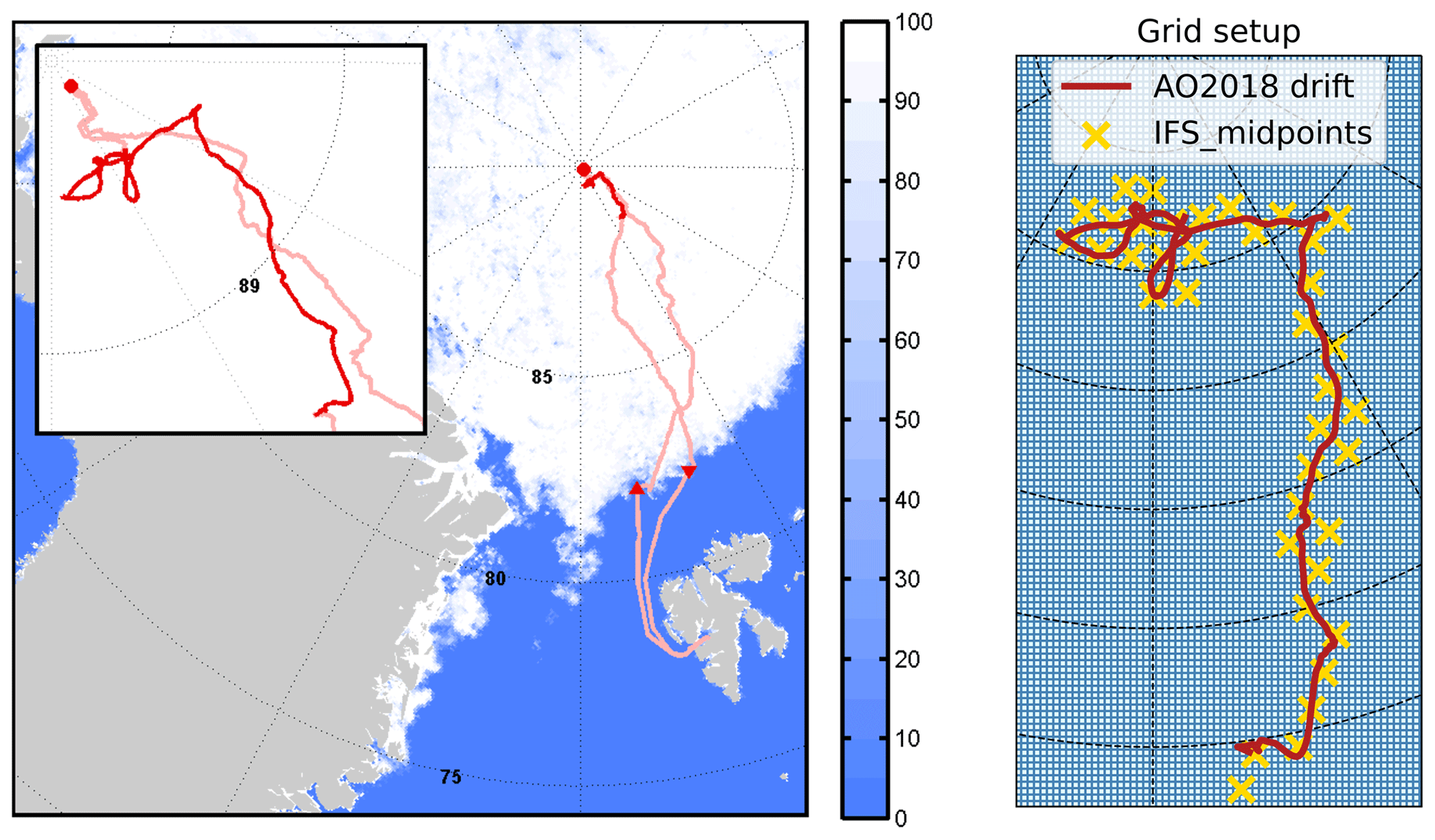
Figure 1Left: map of the cruise track and sea ice cover during the AO2018 expedition from Vüllers et al. (2021), with the drift period (red) in the inset. Right: ship position during the drift period (red), with the grid outline for UM_CASIM-100, UM_RA2T, and UM_RA2M shown in blue and mid-points of the ECMWF_IFS grid indicated by yellow crosses. Note that the grid size difference is for illustrative purposes and is not to scale: UM grid boxes are 1.5 × 1.5 km, and IFS grid boxes are 9 × 9 km in size.
Radiosondes (Vaisala RS92) launched at 00:00, 06:00, 12:00, and 18:00 UTC provide in situ thermodynamic profiles with a 0.5 ∘C and 5 % manufacturer-specified uncertainty associated with temperature and humidity sensors, respectively. The radiosonde data were distributed via the global telecommunications system and assimilated operationally at the Met Office and ECMWF. Remote-sensing measurements from a Metek MIRA-35 Doppler cloud radar, a Halo Photonics Streamline Doppler lidar, and an RPG HATPRO microwave radiometer were processed through the Cloudnet algorithm (Illingworth et al., 2007) following the data-preparation steps of Achtert et al. (2020). A Vaisala PWD22 present-weather sensor (PWS) measured visibility, precipitation type, precipitation intensity, and cumulative amount; near-surface temperature and relative humidity (RH) were obtained from an aspirated Rotronic HMP101 sensor. Broadband downwelling solar and infrared radiation was measured aboard the ship by an Eppley Precision Spectral Pyranometer (PSP) and Precision Infrared Radiometer (PIR). Three-hourly albedo estimates from surface images were used to calculate upwelling shortwave radiation (Vüllers et al., 2021).
2.2 Cloudnet
Cloudnet is used to directly compare between our measured and modelled cloud properties (Illingworth et al., 2007). Cloudnet ingests Doppler cloud radar and lidar, ceilometer, microwave radiometer, and radiosonde data to derive cloud fractions and cloud water contents on a chosen model grid. A comprehensive description of the algorithm is beyond the scope of this paper and is provided by Illingworth et al. (2007) and the references therein, but essentially the algorithm first homogenises observational data to a common time resolution of 30 s and interpolates data to the radar height grid. Radar reflectivity (Ze) and lidar backscatter (β) profiles are used to determine cloud boundaries. Cloudnet takes advantage of the lidar's sensitivity to small particles, such as cloud droplets and aerosol, and the radar's sensitivity to large particles, such as ice particles, rain, and drizzle. Cloud phase is determined using Ze, β, and thermodynamic information from the radiosondes. Cloud ice water content (IWC) is derived using Ze and temperature (Illingworth et al., 2007), while liquid water content (LWC) is derived by partitioning the LWP measured by the radiometer to the identified liquid cloud layers from the lidar. Additionally, an adiabatic LWC is calculated from temperature and humidity profiles and the identified cloud top and base height from radar and lidar measurements.
Cloudnet has already been utilised to study Arctic cloud properties using measurements made aboard Oden during both this campaign (Vüllers et al., 2021) and the Arctic Clouds in Summer Experiment in 2014 (Achtert et al., 2020). Potential errors associated with the Cloudnet procedure are described in Achtert et al. (2020). One particular limitation relevant to this study is the minimum detection height of 156 m (lowest radar range gate). Low-level clouds/fog below this height are hence missed by Cloudnet (Vüllers et al., 2021) and are not included in model comparisons. This limitation also results in problems with the LWC derived from radiometer measurements; therefore, we use the calculated LWC under adiabatic assumption in this study (for further details, see Appendix A).
For comparisons with models, cloud fraction by volume (CV), adiabatic LWC, and cloud IWC from observations are averaged to a reference model grid; here, we use the UM grid, but we could have equally chosen that of the IFS (Fig. S1). Cloud properties are calculated using measurement profiles alongside model wind speed and grid-box size, where changes in cloud properties over time are assumed to be driven primarily by advection and not microphysical changes (Illingworth et al., 2007). This procedure is applied for CV, LWC, and IWC, with CV defined as the fraction of pixels in a 2D slice which are categorised as liquid, supercooled liquid, or ice (Illingworth et al., 2007).
2.3 Models
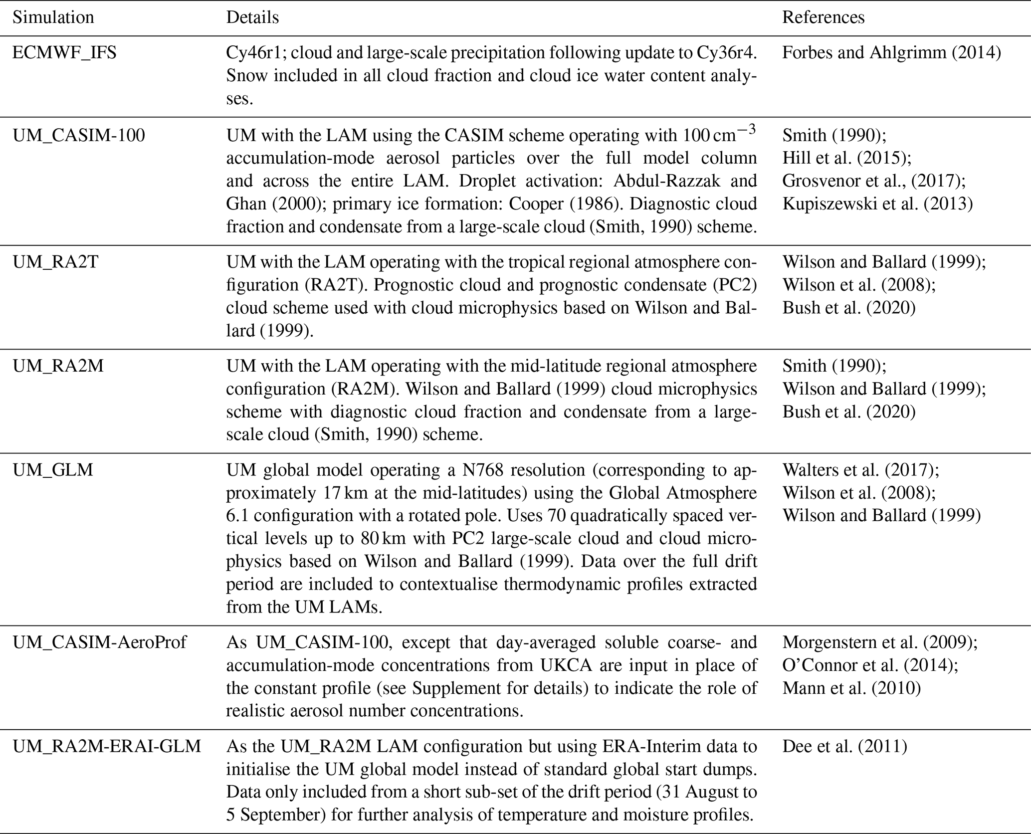
A summary of each model simulation is included in Table 1 and detailed in the following sections; 36 h forecasts were performed with each model, initialised each day at 12:00 UTC with the first 12 h of spin-up discarded, thereby producing daily forecast products (00:00–00:00 UTC) with hourly diagnostics for analysis. This is common practice for such forecasts to ensure discrepancies due to spin-up are avoided while maintaining meteorology close to reality; however, as noted by Tjernström et al. (2021), model error growth is often a function of forecast time, and thus the findings of this study may be related to the time window chosen for each model forecast.
Table 1Summary of the four model configurations to simulate cloud and thermodynamic conditions observed over the full AO2018 drift period in this study. Three additional simulations included for further investigation of results are listed in the shaded sections below.
Column diagnostics from the grid cell closest to the position of Oden were extracted from the model domain, updated hourly to account for the ship's drifting position. These variables (e.g. temperature, humidity, cloud fraction, condensate variables, wind versus time) were then used for comparisons with alike variables constructed using Cloudnet (Illingworth et al., 2007) with measured data (see Sect. 2.1).
2.3.1 IFS; ECMWF_IFS
Cycle 46r1 (Cy46r1) of the IFS (used operationally from June 2019 to June 2020) was used to create global meteorological forecasts. The IFS uses a spectral formulation with a wave-number cut-off corresponding to a horizontal grid size of approximately 9 km (Fig. 1b). It has 137 levels in the vertical up to 80 km, the lowest at ≈10 m, with 8 levels below ≈200 m and 20 below 1 km. IFS forecasts were initialised from ECMWF operational analyses. Operational forecasts produced at the time of the campaign (with Cy45r1) were recently evaluated on a 3 d lead time from a statistical viewpoint for this expedition (Tjernström et al., 2021); in contrast, lead-time-averaged verification was conducted in this study using a 1 : 1 comparison of a concatenated time series of forecast values (forecast time; T+13–T+36) with hourly observations.
Cloud properties are parameterised following Forbes and Ahlgrimm (2014). This cloud scheme was implemented in Cy36r4 and has been previously evaluated for Arctic clouds by Sotiropoulou et al. (2016) using Cy40r1. Five independent prognostic cloud variables are included (grid-box fractional cloud cover and specific water contents for liquid, rain, ice, and snow). Heterogeneous primary ice formation is diagnosed following Meyers et al. (1992), with a mixed-phase cut-off of −23 ∘C. Liquid cloud formation occurs when the average relative humidity within a grid box exceeds a critical threshold, RHcrit, representing sub-grid-scale variability of moisture. This threshold is 80 % in the free troposphere, increasing towards the surface in the boundary layer (Tiedtke, 1993). Once formed, cloud liquid mass is distributed across a fixed cloud droplet number concentration, Nd, of 50 cm−3 over the ocean (and 300 cm−3 over land) to act as a threshold for autoconversion from liquid to rain. For interactions with the radiation scheme, the IFS follows Martin et al. (1994) for estimating droplet number, using the prognostic specific liquid water content and a prescribed CCN profile. CCN concentrations are calculated as a function of the near-surface wind speed but decrease with altitude to represent the vertical distribution of aerosol within and above the BL. Further details regarding the cloud scheme can be found in the ECMWF documentation (IFS Documentation – Chapter 7: Clouds and large-scale precipitation, https://www.ecmwf.int/node/19308, last access: 10 August 2022).
The IFS is coupled to a 0.25∘-resolution dynamic sea ice model (Louvain-la-Neuve Sea Ice Model, LIM2) which provides sea ice fractions to the IFS and the surface flux tiling scheme (Buizza et al., 2017; Keeley and Mogensen, 2018). The surface energy balance over the sea ice fraction is, however, calculated separately from LIM2 using an albedo parameterisation following Ebert and Curry (1993) with fixed monthly climatology values interpolated to the actual time and a heat flux through the ice calculated using a constant sea ice thickness of 1.5 m.
2.3.2 UM
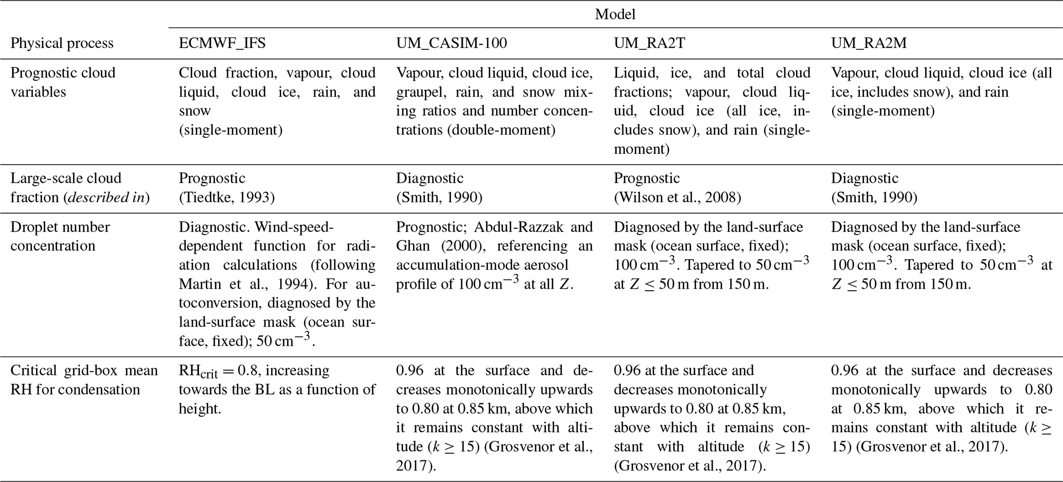
The UM was operated as a high-resolution LAM with a 1.5 km × 1.5 km grid (the grid is shown in Fig. 1). A rotated pole configuration provided approximately equal spacing between grid points towards 90∘ N. The LAM contained 500 × 500 grid boxes, spanning from 83.25 to 90∘ N centred on the 30∘ E meridian. In the vertical, there were 70 vertical levels up to 40 km, with 24 levels within the lowest 2 km of the domain (Grosvenor et al., 2017). Lateral boundary conditions were generated hourly from UM global model 36 h forecasts at N768 resolution (corresponding to approximately 17 km at 90∘ N with the rotated pole) using the Global Atmosphere 6.1 configuration (Walters et al., 2017; Table 1). Three configurations of the UM LAM were tested for the main body of this study, each using different combinations of cloud microphysics and large-scale cloud schemes. Each simulation uses the same boundary layer scheme, where mixing in the vertical is described by Lock et al. (2000); however, one must note that turbulent interactions can be influenced by the relationship between cloud-top radiative cooling and subsequent convective overturning with cloud microphysics. Details on the pertinent microphysical processes represented in each simulation are listed in Table 2.
Table 2Summary of cloud microphysical process representation in each simulation set-up. Chosen processes are highlighted as key differences between the schemes. k: model level; Z: altitude.
Regional Atmosphere model configurations (UM_RA2M and UM_RA2T)
Version 2 of the Regional Atmosphere model within the UM framework has two standard configurations: the mid-latitude configuration (UM_RA2M) and the tropical configuration (UM_RA2T). Both are used operationally in their respective geographical regions. The key difference between these configurations can be found in their turbulent mixing processes: UM_RA2M employs weak turbulent mixing to encourage heterogeneity in model fields to facilitate the triggering of small convective showers; however, while this weak mixing works well to reproduce conditions often experienced at the mid-latitudes, it triggers convection too early in the tropics. Therefore, these two standard Regional Atmosphere configurations were designed separately to account for these subtle differences in convection initiation on kilometre scales (Bush et al., 2020).
Neither configuration has been previously evaluated for use in the Arctic. Note that both UM_RA2M and UM_RA2T use the default Regional Atmosphere surface albedo thresholds, giving a 50 % albedo at an ice surface temperature of 0 ∘C and increasing to 80 % at −10 ∘C. Gilbert et al. (2020) tested both configurations for polar cloud modelling over the Antarctic Peninsula, finding that the mid-latitude scheme performs better than the tropical configuration for capturing polar cloud liquid water properties and the associated radiative interactions (with the surface albedo modelled to within 2 % of the observed values), whereas the tropical scheme enabled a too-efficient ice phase (and associated liquid depletion).
Both UM_RA2M and UM_RA2T include the Wilson and Ballard (1999) description of large-scale precipitation to simulate resolved cloud microphysics. This microphysics scheme describes prognostic liquid and ice mixing ratios (qliq and qice, respectively), with an assumed fixed Nd profile calculated from an aerosol climatology and tapered to 50 cm−3 towards the surface (between 150 and 50 m). A single ice species (encapsulating pristine crystals, aggregates, and snow particles) is represented, with an assumed particle size distribution based on Field et al. (2007).
UM_RA2M uses the Smith (1990) large-scale cloud scheme to parameterise sub-grid-scale fluctuations in humidity and cloud, designed to ensure coarse-grid GCMs do not have entirely cloudy grid boxes. IWC is fixed for a given temperature, and only the total cloud fraction is represented. Smith (1990) diagnoses cloud fraction and condensate variables for input to the microphysics scheme, referencing a prescribed RHcrit profile (based on a symmetric triangular probability density function of sub-grid-scale variability in temperature and moisture) to permit condensation below 100 % humidity (Wilson et al., 2008). Condensation cannot occur within a grid box until the grid-box mean RH exceeds RHcrit (described in Table 2).
In UM_RA2T, the prognostic cloud fraction and prognostic condensate (PC2; Wilson et al., 2008) large-scale cloud scheme is used, designed to address the over-sensitive diagnostic links between cloud fraction and cloud condensate in Smith (1990). Total, liquid, and ice cloud fractions are included as prognostic variables in PC2; ice cloud fraction is calculated from a prognostic ice mass mixing ratio, with a distribution of IWC values possible for the same cloud fraction. Cloud fractions and condensate can vary through other interactions (such as BL processes and cloud microphysics) and are not simply diagnosed from temperature and humidity as in Smith (1990) (Wilson et al., 2008). PC2 prognostic variables are advected by the wind and continually updated following incremented sources and sinks in the model, with the additional inclusion of sub-grid-scale turbulent production of liquid in mixed-phase cloud from an analytical model of sub-grid-scale moisture variability (Furtado et al., 2016). Differences between the methods of representing cloud fraction in the PC2 and Smith schemes are detailed in the Supplement.
Regional Atmosphere with the Cloud-Aerosol Interactive Microphysics scheme (UM_CASIM-100)
UM_CASIM-100 uses the CASIM scheme (detailed by Hill et al., 2015) coupled with the Smith (1990) large-scale cloud scheme (as in Grosvenor et al., 2017). Stevens et al. (2017) previously tested the CASIM scheme within the UM nesting suite in an Arctic cloud case study, showing that it performed well in capturing cloud dissipation; however, the authors did not include sub-grid-scale contributions from Smith (1990) in that study.
CASIM utilises prescribed log-normal aerosol distributions to provide a double-moment representation of cloud particle processes and is the only double-moment set-up included in this study. Particle size distributions of five hydrometeors (liquid droplets, ice, snow, graupel, and rain) are each described by a gamma distribution, with prognostic mass mixing ratios and number concentrations. Ice number concentrations are diagnosed via a temperature–number concentration parameterisation (Cooper, 1986) but require liquid to be present before ice can form, a relationship thought to be important in Arctic mixed-phase clouds (e.g. de Boer et al., 2011; Young et al., 2017). Droplet activation follows Abdul-Razzak and Ghan (2000), referencing a fixed soluble accumulation-mode aerosol number concentration profile of 100 cm−3. This profile was approximated based on aerosol concentration profiles previously measured during summertime in the central Arctic (Kupiszewski et al., 2013).
CASIM offers user flexibility regarding aerosol processing, as described by Miltenberger et al. (2018). Here we do not impose wet-scavenging processes, likely important for capturing cloud-free conditions, for consistency with the simpler single-moment liquid microphysics schemes used in the other simulations; however, use of this option will be explored in future work.
For our CASIM simulation, we adapt the warm ice temperature albedo of the LAM to 72 % (at 0 ∘C), with 80 % albedo achieved at −2 ∘C, to match the parameterisation limits currently used in the JULES (Joint UK Land Environment Simulator) surface scheme of the Global Atmosphere 6.0 global model (under the assumption that snow is present on the sea ice surface). For the drift period, we know that snow was indeed present on the surface from first-hand knowledge and surface imagery; therefore, we use this simulation to test the effect of such an increased albedo at warmer surface ice temperatures on the modelled surface energy balance. An example simulation utilising the CASIM scheme with the default Regional Atmosphere albedo settings used in UM_RA2M and UM_RA2T, to demonstrate the radiative impact of CASIM alone, is described in the Supplement (Sect. S2).
2.4 Comparison methodology and compared parameters
CV, qliq, and qice from each model simulation were ingested by Cloudnet to calculate LWC and IWC. Within these calculations, Cloudnet filters model data for values outside the range observable by the instrumentation used; for example, qice data are filtered for values which would be beyond the observable range of the radar.
We use an additional metric alongside CV based on total condensate for comparisons between our measured and modelled clouds, a total water content (TWC) mask where the grid box is considered cloudy. This mask is set to 1, when kg m−3 below 1 km and kg m−3 above 4 km, with vertical interpolation in between (following Tjernström et al., 2021; Fig. S3). While this mask will not capture fractional cloud at cloud boundaries, averages of this mask are directly comparable between the observations and models. It acts as a comparison metric based solely on cloud water contents, which are prognostic in every simulation, and does not depend on a specific definition of e.g. cloud fraction.
In addition to a full overview of model performance over the drift, we further split our data into sub-periods to aid our interpretation of the comparisons between the measurements and models. The sea ice melt–freeze transition was captured by the measurements; Vüllers et al. (2021) identified the sea ice freeze onset date as 28 August and defined sub-periods throughout the drift based on consistent meteorology (see Fig. 2g). We concentrate on the sea ice melt and freeze periods separately and on shorter episodes within these periods, one during the sea ice melt (14–18 August) and one during the freeze (4–8 September).
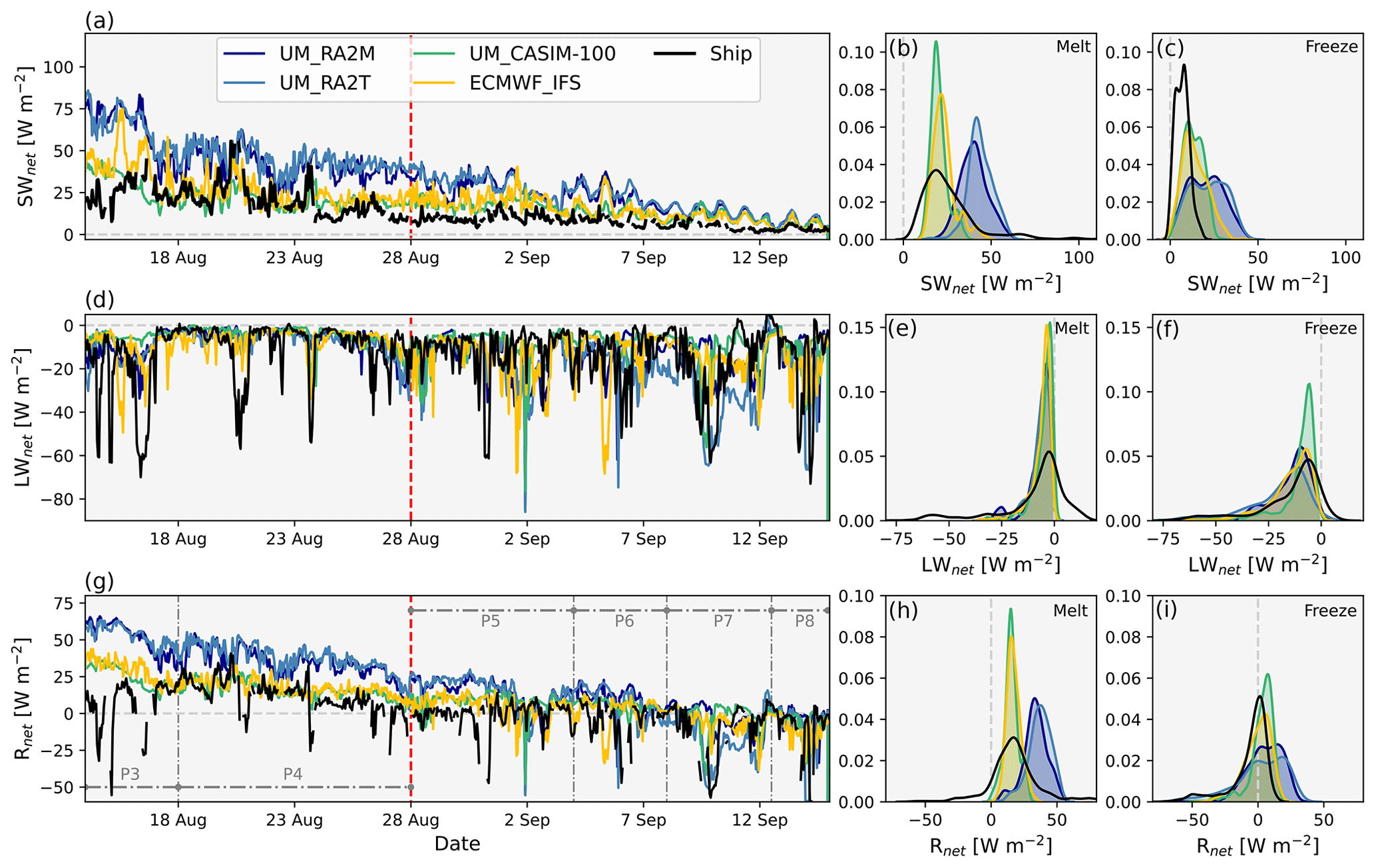
Figure 2SWnet, LWnet, and Rnet simulated by UM_RA2M (dark blue), UM_RA2T (light blue), UM_CASIM-100 (green), and ECMWF_IFS (yellow). Hourly averaged measurements aboard the ship (black) shown for comparison. Left: time series. Right: PDFs. PDFs are split between melting and freezing sea ice conditions using a threshold of 28 August as indicated by the red vertical dashed line in panels (a), (d), and (g). Radiation terms are defined as positive downwards. Sub-periods used in subsequent sections are marked (grey) in panel (g).
3.1 Surface radiation
Figure 2 shows measured and modelled time series of net surface shortwave (SWnet) radiation, LWnet, and the combined surface net radiation (Rnet) during the AO2018 drift period. All radiative quantities are defined as positive downwards.
All the models overestimate SWnet (Fig. 2a) with respect to measurements, with ECMWF_IFS and UM_CASIM-100 in better agreement with observations than UM_RA2M and UM_RA2T. From Fig. 2d, all the simulations fail to capture strong longwave net emission likely related to cloud-free episodes (e.g. 20–21 August) and sporadically predict such cloud-free conditions (and net longwave emission) when clouds were observed (e.g. 2 September).
Considering the melt and freeze periods separately, the measured Rnet is often negative after 28 August (Fig. 2g), driven by LWnet, while SWnet decreases with the declining solar elevation angle (Fig. 2a). In contrast, the models' net radiation is not typically negative until after 8–9 September, excluding a short negative period on 2 September driven by the lack of modelled cloud (as suggested by strong net longwave emission; Fig. 2d). This delay would likely affect the freeze onset if the models were fully coupled to a sea ice model; as such, this feedback may be active within the (simple) coupled atmosphere–sea ice system of the IFS.
Probability density functions (PDFs) of these data, split between melt and freeze periods (Fig. 2b–c, e–f, h–i), reveal some clear distinctions in model capability. SWnet PDFs vary substantially between the models during the melt period (Fig. 2b); no simulation captures the observation distribution well. Observed SWnet from the ship has a median of +18.2 W m−2, with each simulation producing medians at greater values (UM_CASIM-100 W m−2; ECMWF_IFS W m−2; UM_RA2M W m−2; UM_RA2T W m−2). While the medians for UM_CASIM-100 and ECMWF_IFS are in good agreement with observations, both exhibit a too-narrow distribution. These too-narrow distributions – which also all lack a very high positive tail – suggest that the modelled cloud cover is too consistent, likely related to the lack of cloud-free episodes indicated by the LWnet data (Fig. 2d). The median SWnet of both the UM_RA2T and UM_RA2M PDFs is much too high, with non-negligible occurrences >+50 W m−2. The improvement of UM_CASIM-100 over UM_RA2T and UM_RA2M indicates that the surface albedo used by default in the Regional Atmosphere configurations is too low, and the updated cloud physics description of CASIM improves the modelled cloud–radiation interactions. A trial simulation utilising the cloud physics set-up of UM_CASIM-100 alongside the default Regional Atmosphere surface albedo parameterisation inputs (as used in UM_RA2M and UM_RA2T) shows that the double-moment cloud physics representation alone does improve radiative properties in comparison to the standard configurations (see Supplement); however, the combination of improved cloud–radiation interactions and an updated surface albedo (as shown here in UM_CASIM-100) provides the best agreement between the UM and our observations.
During the freeze period, measurement estimates of SWnet peak at +7.9 W m−2, while ECMWF_IFS, UM_CASIM-100, UM_RA2M, and UM_RA2T have maxima at +10.0, +10.4, +25.0, and +26.6 W m−2, respectively (Fig. 2c). The peak modelled SWnet remains too high in all the simulations, but, in contrast to the melt period, all PDFs are now too broad. ECMWF_IFS and UM_CASIM-100 perform best with comparison to observations (both with a positive bias of less than +3 W m−2 at their peaks). However, both UM_RA2M and UM_RA2T have a broad bimodal structure, with the secondary peak in better agreement with the observations than their maxima. Both UM_RA2T and UM_RA2M are largely in better agreement with observations during the freeze period than during the melt; this improved agreement is likely due to either a better representation of incoming shortwave radiation or the surface albedo. The surface temperatures decrease through the transition to sea ice freezing conditions, and Fig. S4 indeed shows that the albedo modelled during the freeze for UM_RA2M and UM_RA2T is in better agreement with observational estimates than that modelled during the melt period.
During the melt period, LWnet aligns well between the measurements and models; however, all the simulations produce a narrower PDF than the observations and largely miss the tail <−20 W m−2 (Fig. 2e) resulting from observed cloud-free episodes on 15–16, 20, 22, and 26 August (Fig. 2d). Despite this, each simulation performs well in replicating the median of the PDF, with a maximum model–observation difference of −1.9 W m−2 (UM_RA2T). As with SWnet, model–observation agreement generally improves during the freeze period, with UM_RA2M, UM_RA2T, and ECMWF_IFS producing PDFs closely matching the shape of the observed PDF, with median values at −9.4, −11.5, and −6.8 W m−2, respectively, compared with an observation peak of −6.5 W m−2 from the ship estimates. Each of these cases manages to reproduce the negative distribution tail missed by all the simulations during the melt (Fig. 2f). UM_CASIM-100 displays a narrower distribution with fewer negative values yet still performs well in reproducing the median of the LWnet PDF (with a bias of −5.5 W m−2). With the exception of the too-narrow UM_CASIM-100 PDF, this improved agreement in LWnet indicates that cloud cover is indeed captured better by the models during the freeze, and remaining discrepancies in the SWnet comparisons may indeed be related more so to cloud microphysical structure or surface properties.
To investigate this relationship in more detail, we split our radiation data into periods of consistent meteorology, indicated in Fig. 2g, based on similarity of equivalent potential temperature and relative humidity profiles measured as defined in Vüllers et al. (2021). In agreement with Fig. 2, model SWnet and downwelling shortwave radiation (SW↓) biases are at their greatest during period 3 (Table 3).
Table 3Mean surface radiation biases (model–observation) over periods 3–6, with mean measured values for reference. Observations included are hourly integrated values for consistency with the models. All values are in Watt per square metre. The smallest biases are highlighted in bold.
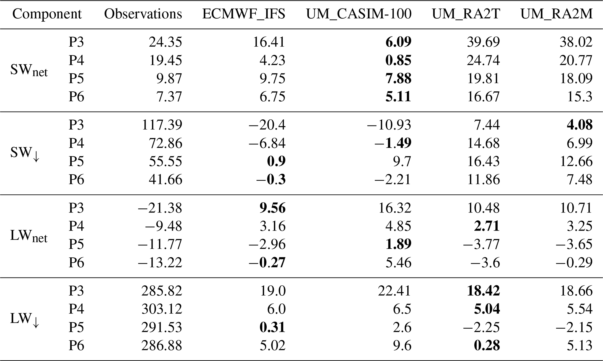
Each of these simulations highlight that small SW↓ biases do not necessarily produce similarly small SWnet biases, as both the modelled cloud properties and surface albedo need to be representative to remedy the SWnet discrepancies. In UM_RA2T and UM_RA2M, the surface albedo is poorly captured, as indicated by the consistently high SWnet biases; however, ECMWF_IFS and UM_CASIM-100 perform better in terms of surface albedo, with UM_CASIM-100 performing the best with the smallest SWnet biases across the four sub-periods considered. Further discussion of the surface albedo comparison is included in the Supplement.
All the simulations exhibit their greatest LWnet biases during period 3 (Table 3); less cloud cover was observed during this period in relation to other periods during the drift (Vüllers et al., 2021). LWnet biases do not exceed +5.5 W m−2 over periods 4–6; however, biases are greater (up to +16.3 W m−2 during period 3; Table 3) due to the models' inability to reproduce cloud-free conditions.
Combining these radiative components, we find that Rnet is overestimated by all the simulations during the melt (with UM_CASIM-100 and ECMWF_IFS performing better than UM_RA2M and UM_RA2T; Fig. 2h), largely driven by too much surface SWnet modelled when cloud is present in reality, thus indicating that the model surface albedo is too low and thus does not reflect enough SW↓. On the other hand, there are also non-negligible occurrences of too much modelled cloud when the conditions should be cloud-free, driving strong LWnet biases at these times. While agreement with observations largely improves during the freeze period, these discrepancies still exist in the SWnet data. While the SWnet biases may be strongly influenced by errors in the surface albedo and thus beyond the scope of this study, the role of cloud structure in SW↓ biases and the LWnet emission episodes missed by each simulation are driven by the description of cloud: in the following sections, we investigate the cloud macrophysical and microphysical structure to explain these radiative differences.
3.2 Cloud properties
To evaluate model performance, we use two metrics for cloud occurrence: the model-diagnosed cloud fraction, CV, and the cloud occurrence inferred from cloud water contents, the TWC cloud mask. Figure 3 shows TWC and cloud fraction, CV, calculated from observations using Cloudnet and output by models. TWC comparisons indicate that each simulation captures the observed cloud aloft, except for UM_CASIM-100 between 4 and 10 September. Below 3 km, observed TWC is generally lower in magnitude than the model simulations.
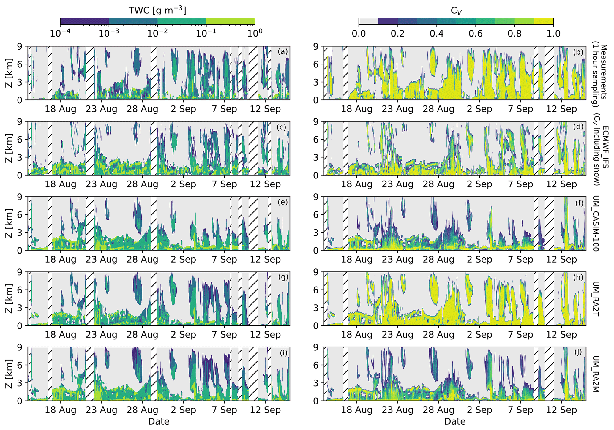
Figure 3Total water content (left, TWC) and cloud fraction (right, CV). Panels (a–b) are calculated from observations using Cloudnet and diagnosed by (c–d) ECMWF_IFS, (e–f) UM_CASIM-100, (g–h) UM_RA2T, and (i–j) UM_RA2M. Missing measurement data are indicated by hatched areas; times where data are missing from the observations are removed from the model data to provide a fair comparison. Missing data periods differ between the TWC and CV products due to the different instrumentation requirements within Cloudnet for each.
In contrast, all the simulations except UM_RA2T fail to reproduce the observed CV aloft. Low-altitude (below 2 km) cloud cover appears to be captured comparatively better across all the simulations. Cloud height simulated by ECMWF_IFS is in reasonable agreement with the observations; however, there are notable periods where the persistence of clouds aloft is not reproduced. For example, the altitude and timing of the onset of the (likely precipitating) high clouds on 3–4 September are initially captured, but the clouds are not sustained. Cloud layers aloft appear more tenuous also in UM_RA2M and UM_CASIM-100 than in the observations: there are few cases of cloud fractions >0.5 at altitudes above 3 km.
Figure 4a shows mean profiles of CV over the drift period. Only periods where we have measurement data are included in these profiles for fair comparison. Note that cloud fraction below 0.15 km is not evaluated against observations here due to the low-altitude measurement limit of the cloud radar. Supporting qualitative interpretation of Fig. 3, model–observation agreement of CV is best at low altitudes (below 1 km); however, all the simulations produce too much very-low (between 0.15 and 0.5 km) cloud. Modelled near-surface CV (between 0.15 and 0.5 km) is up to 16 % too high (UM_RA2T). However, we can speculate that the frequent fog episodes reported during the ice drift (Vüllers et al., 2021) may be somewhat captured by the models, as indicated by mean values of CV below 0.15 km of 82 %, 72 %, 53 %, and 39 %, respectively, for UM_RA2T, UM_RA2M, UM_CASIM-100, and ECMWF_IFS. All the simulations except UM_RA2T perform poorly aloft: ECMWF_IFS, UM_RA2M, and UM_CASIM-100 strongly underestimate CV between 1 and 8 km, with UM_CASIM-100 and UM_RA2M reproducing less than 20 % of the observed CV at 4.5 km. Only the UM_RA2T CV profile agrees well at altitude, with particularly good agreement between 0.5 and 2 km – in fact, CV between 2 and 5.5 km agrees best with observations out of the four simulations considered.

Figure 4Comparison between (a) mean CV observed (black, calculated using Cloudnet) and modelled (UM_RA2M in dark blue, ECMWF_IFS in yellow, UM_CASIM-100 in green, UM_RA2T in light blue) over the AO2018 drift period. (b) TWC cloud mask comparison, where masks are calculated using only in-cloud data as described in Sect. 2.4. (c–d) Same comparison for liquid and ice cloud water contents, respectively, using in-cloud data only. LWC data from the observations are calculated using Cloudnet by assuming an adiabatic profile (see Appendix A). Lines indicate the mean profiles of each dataset, and shaded areas depict ± 1 standard deviation from the mean. Uncertainties associated with the retrieval process are not shown.
Figure 3 highlights that the observations, UM_RA2T, and (to an extent) ECMWF_IFS have a CV field scaling largely as either 0 or 1, whereas UM_RA2M and UM_CASIM-100 are more likely to have a fractional cloud cover aloft, thus producing a poor comparison with our observations (Fig. 4a). Despite this, qualitative model–observation comparisons of TWC indicate that the models are performing well. Further discussion of these differences is included in the Supplement. In summary, the Cloudnet calculation of CV from observations is not directly equivalent to our model cloud fractions, and such comparisons, in isolation, should be approached with caution in the Arctic. To bypass this issue, we also use a cloud mask built from TWC data to aid interpretation of our results. The observed TWC cloud mask (Fig. 4b) differs from the mean CV profile, with a subtle bimodal structure peaking at approximately 0.5 and 4.5 km (with a minimum around 2 km).
All the simulations overestimate cloud occurrence below 2.5 km (Fig. 4b), in contrast to the underestimation between 1 and 2.5 km shown in the CV data (Fig. 4a). Mean observed cloud occurrence only reaches 75 % between 0.15 km (lowest radar range gate) and 0.5 km, while UM_RA2M and UM_CASIM-100 have more than 98 % cloud occurrence at 0.2 km. UM_RA2T performs slightly better, peaking to only 92 % at 0.2 km; however, the improvement is not as significant between UM_RA2T and UM_RA2M/UM_CASIM-100, as is suggested by the mean CV profiles (Fig. 4a). ECMWF_IFS peaks at a slightly higher altitude, overestimating cloud occurrence by 33 % at approximately 0.5 km (Fig. 4b).
Above 2 km, each model simulation underestimates the observed cloud occurrence, in line with the CV metric comparison. ECMWF_IFS, UM_RA2M, and UM_RA2T perform similarly; the greatest difference aloft occurs at 4.5 km, where there is a minor peak in the mean observed cloud occurrence (up to 41 %; Fig. 4b). ECMWF_IFS produces only 28 % cloud cover at this altitude. UM_CASIM-100 cloud occurrence monotonically decreases with altitude above 3.5 km, producing only 20 % cloud cover at 4.5 km, in agreement with the qualitative findings of Fig. 3. Therefore, with the exception of UM_CASIM-100, the TWC cloud mask indicates that modelled cloud occurrence aloft is, in fact, in reasonable agreement with observations, in contrast to the trends indicated by the CV data (Fig. 4a). These data suggest that the CV comparisons are misleading if used in isolation, likely due to the different methods for representing cloud fractions and associated sub-grid-scale variability in models (see Supplement). Cloud masks constructed from cloud water contents provide a more consistent metric between observations and models.
Averaged in-cloud water content profiles are shown in Fig. 4c–d. Adiabatic LWC calculated from observations with Cloudnet is shown in Fig. 4c. This adiabatic assumption was used in place of the HATPRO LWP due to the data quality issues introduced to the latter because of the frequent occurrence of fog at altitudes below the lowest radar range gate (0.15 km, discussed further in Appendix A). However, we must note that this assumption likely overestimates the observed LWC as these clouds are likely sub-adiabatic.
The adiabatic LWC peaks between 0.5 and 1 km then decreases steadily with altitude between 1 and 3 km. All the simulations overestimate in-cloud LWC between 1 and 3 km; however, below 1 km, each simulation (except UM_RA2T) performs reasonably well. At 0.5 km, UM_RA2T underestimates it by 47 %, while UM_CASIM-100 overestimates it by just 10 %, and UM_RA2M and ECMWF_IFS are in reasonable agreement with observations. UM_RA2T and UM_RA2M have bimodal distributions, with peaks below 0.5 and around 2 km, perhaps linked to their common use of the Wilson and Ballard (1999) microphysics scheme. The increase in LWC towards the surface in UM_RA2M is suggestive of fog, and UM_RA2M is the only simulation to display this vertical structure. The mean LWC calculated for ECMWF_IFS does not vary greatly between 0.5 and 2 km; however, there is more spread in the data at 2 km than at lower altitudes, indicating that this may be a more dominant liquid cloud layer occurring at some time periods. Only UM_CASIM-100 displays a similar shape to the observations, yet its LWC is often greater than the observed LWC at all altitudes above 1 km. Considering that we employ an adiabatic assumption for our observations, thereby giving an upper limit for the observed LWC, these model LWC biases are likely greater in reality than shown here.
All the simulations agree with the Cloudnet-calculated mean IWC above 4 km (Fig. 4d); in fact, UM_RA2M performs particularly well across the entire vertical profile. ECMWF_IFS and UM_CASIM-100 also agree well for most of the profile apart from slight overestimations below 1.5 km (though still within 1 standard deviation of the observed mean). UM_RA2T overestimates below 4 km, producing almost 7 times the observed IWC (0.019 g m−3 versus 0.003 g m−3) at 0.5 km. Shaded areas, depicting ± 1 standard deviation from the mean, also indicate that UM_RA2T is also more variable than the three other simulations and the measurements, consistent with previous studies showing that its ice phase is more active than UM_RA2M in polar mixed-phase clouds (Gilbert et al., 2020).
Column-integrated metrics and surface measurements provide an additional perspective for evaluating model performance with regards to clouds. Measured LWP and precipitation fluxes are shown alongside the corresponding model diagnostics in Fig. 5. Cloudnet-filtered LWP is included in Fig. 5a, b for comparison; these data are HATPRO measurements filtered by Cloudnet for bad points (e.g. strong precipitation events). ECMWF_IFS, UM_RA2M, and UM_CASIM-100 produce LWPs in reasonable agreement with measurements throughout the full drift period, with the PDFs of Fig. 5b indicating that these LWPs are overestimated slightly with respect to the measurements/Cloudnet data. UM_RA2M overestimates in some periods: for example, the LWP peak during the storm of 12 September is 230 g m−2 more than measured (Fig. 5a). In contrast, UM_RA2T underestimates the LWP overall, with few occurrences of >200 g m−3 (Fig. 5b). This underestimation of LWC (Fig. 4c) and LWP (Fig. 5a, b) by UM_RA2T aligns with its overestimation of IWC below 4 km; with too much ice in mixed-phase cloud, liquid is depleted too efficiently via the Wegener–Bergeron–Findeisen mechanism.
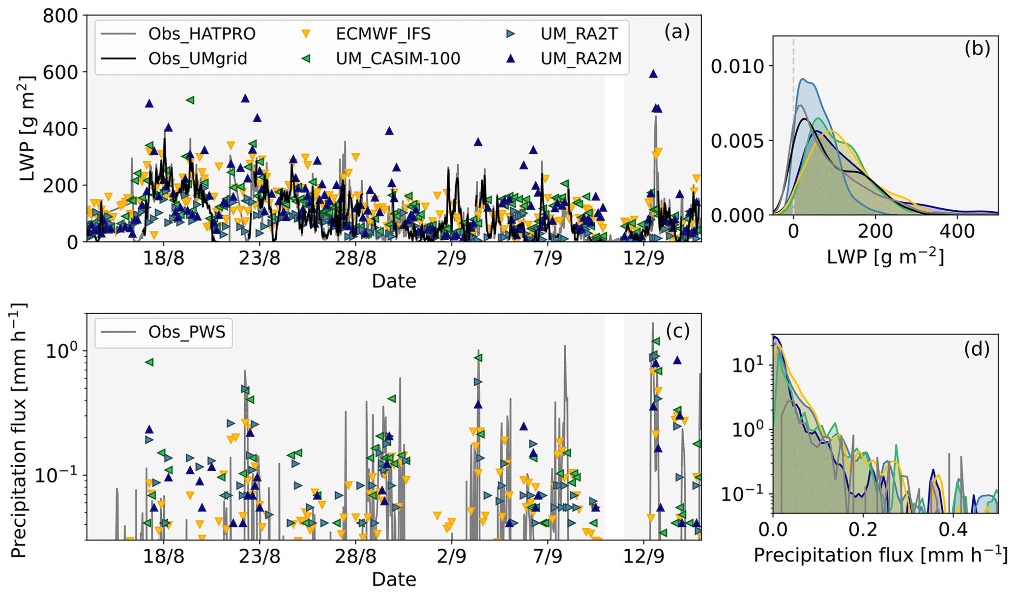
Figure 5Time series of (a–b) liquid water path (LWP) and (c–d) total precipitation flux at the surface over the full drift period. (a–b) HATPRO measurements (grey) are included for comparison with the model data (coloured markers). LWP data averaged onto the UM grid by Cloudnet are shown in black (Obs_UMgrid). (c–d) Weather sensor (PWS) measurements of total precipitation from the seventh deck (grey) are included for comparison with model rain and snow fields. (a, c) Model data shown every 3 h for clarity; (b, d) all model data included for comparison.
Each simulation broadly captures the notable precipitation events measured (Fig. 5c–d). UM_CASIM-100 and UM_RA2T reproduce the measured total precipitation flux well and capture the short episodes where more precipitation was observed on 22 August and 3 and 12 September. ECMWF_IFS and UM_RA2M also capture some precipitation events; however, the magnitude of these events is best reproduced by UM_CASIM-100. No simulation reproduces the precipitation intensity measured on 8 September. While the key precipitation events are largely captured by the models, with each model producing precipitation as predominantly snow rather than rain, the precipitation rates simulated are low and likely contribute to the lack of cloud-free periods as indicated by the LWnet comparisons shown previously (Fig. 2d, e, f).
These results therefore indicate that the modelled microphysical structure is positively biased in terms of cloud liquid with respect to observations (Figs. 4c, d–5). There is a consistent model–observation bias, with all the simulations producing too much cloud (Fig. 4a, b) below 2.5 km. In ECMWF_IFS, UM_RA2M, and UM_CASIM-100, this cloud contains too much liquid (as indicated by positive biases in LWC and LWP). Only UM_RA2T underestimates the cloud liquid properties due to its active ice phase. Figure 6 links the radiation, LWP, and CV biases of our four model simulations with respect to observations. CV biases are calculated as the model–observation bias between 0.15 and 3 km. Here, CV is used in place of the TWC cloud mask as the latter is calculated from in-cloud LWC and is therefore not strictly independent of LWP. Positive CV biases often coincide with positive LWP biases, negative SW↓ biases (Fig. 6a, d, g, j), and positive LW↓ biases (Fig. 6b, e, h, k), and vice versa, indicating that too much cloud cover and too much cloud liquid water are tied to the radiative biases shown. The correlation with LWP bias is weaker for Rnet than for SW↓ or LW↓, likely due to the additional influence of other factors (e.g. surface albedo) on the net radiative properties.
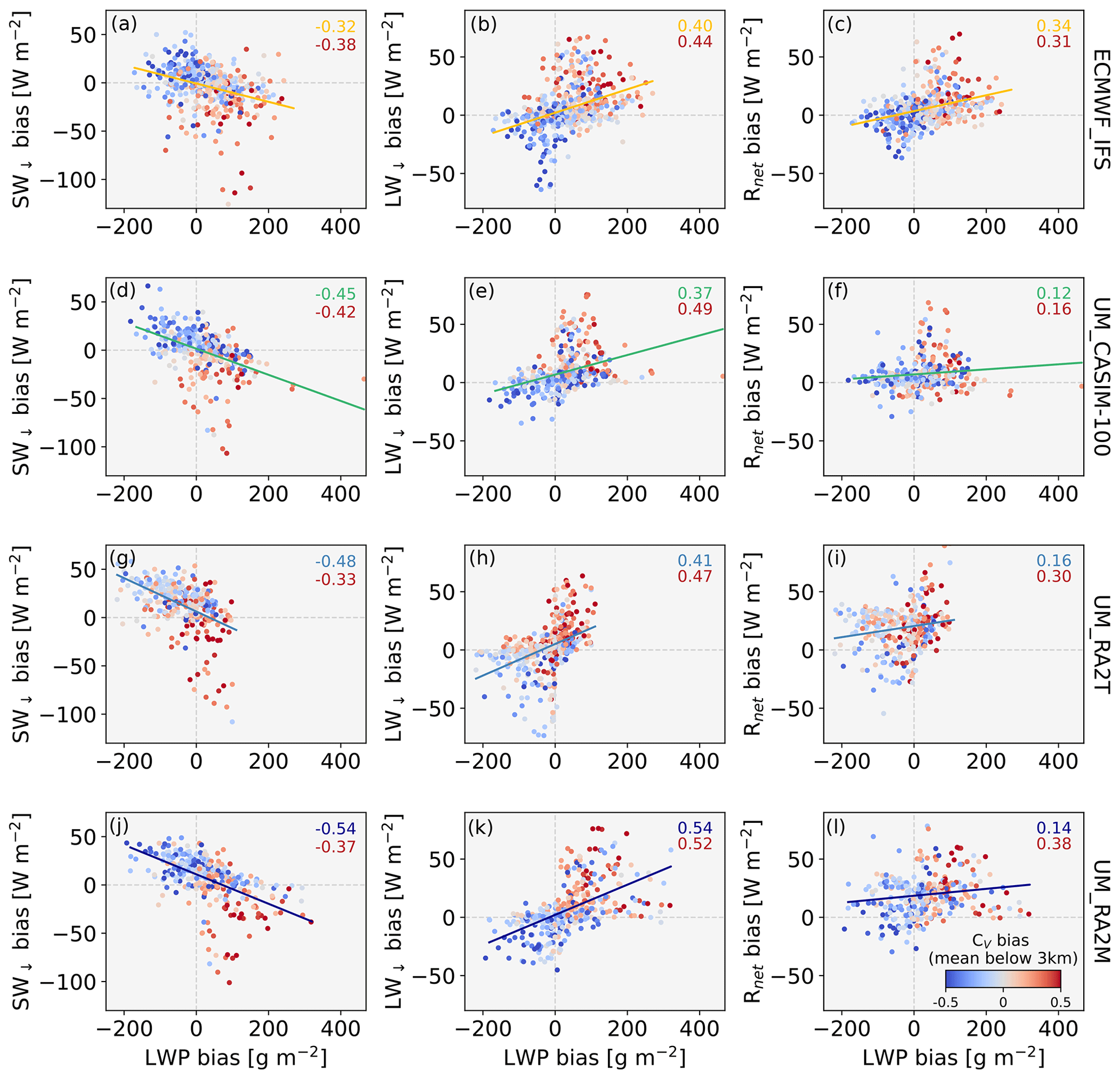
Figure 6Model biases in radiation terms (SW↓ (left), LW↓ (middle), and Rnet (right)), LWP, and CV. Model–observation biases are calculated hourly for the radiation and LWP terms using measurements from the ship-based radiometers and HATPRO microwave radiometer, respectively. Shading: model–observation difference between mean CV below 3 km, where model data below the height of the lowest radar range gate (156 m) are excluded from the comparison with observations. Correlation coefficients for the radiation–LWP (top) and radiation–CV regressions (bottom) are noted in the top right of each panel.
3.2.1 Influence of CCN concentration
Each simulation overestimates cloud occurrence below 2.5 km and struggles to maintain cloud-free conditions, problems previously identified for earlier versions of these models. Both Sotiropoulou et al. (2016) and Birch et al. (2012) commented on the need for variable, representative cloud nuclei concentrations in the IFS and the UM to enable cloud-free periods to be captured. A fixed accumulation-mode aerosol number and mass concentration profile was used in UM_CASIM-100; however, such consistency with altitude is unlikely to occur in reality. While the concentration chosen was based on previous measurements in the Arctic (Kupiszewski et al., 2013), aerosol number concentrations are typically very low and heterogeneous within the BL during the Arctic summer (Mauritsen et al., 2011; Tjernström et al., 2014), while long-range transport provides comparatively greater, more homogeneous concentrations aloft.
An additional simulation with the CASIM scheme was tested using a more representative CCN vertical profile guided by output from the UK Chemistry and Aerosol (UKCA; Morgenstern et al., 2009; O'Connor et al., 2014) global model. Details on the UKCA model configuration used to obtain these aerosol data are included in the Supplement. Using representative aerosol profiles as input to the CASIM scheme (with lower CCN concentrations within the lower troposphere and greater concentrations within the free troposphere, denoted UM_CASIM-AeroProf) affects the SW↓ as expected via the associated influence on Nd and qliq (Fig. 7). UM_CASIM-AeroProf has a mean accumulation-mode number concentration of 18.5 ± 11.4 cm−3 below 500 m which, with comparison to the 100 cm−3 specified for UM_CASIM-100, is more appropriate for the region. As a result, low-altitude (below 1 km) clouds have a significantly lower Nd than in UM_CASIM-100: UM_CASIM-AeroProf has a mean Nd of 20.9 ± 15.9 cm−3 below 500 m, compared with 101.0 ± 40.2 cm−3 in this altitude range for UM_CASIM-100. Such a low Nd is expected from periodic episodes of low CCN in the Arctic BL (Mauritsen et al., 2011); cloud residual concentrations of up to 10 cm−3 were measured aboard Oden during the AO2018 expedition (Baccarini et al., 2020).
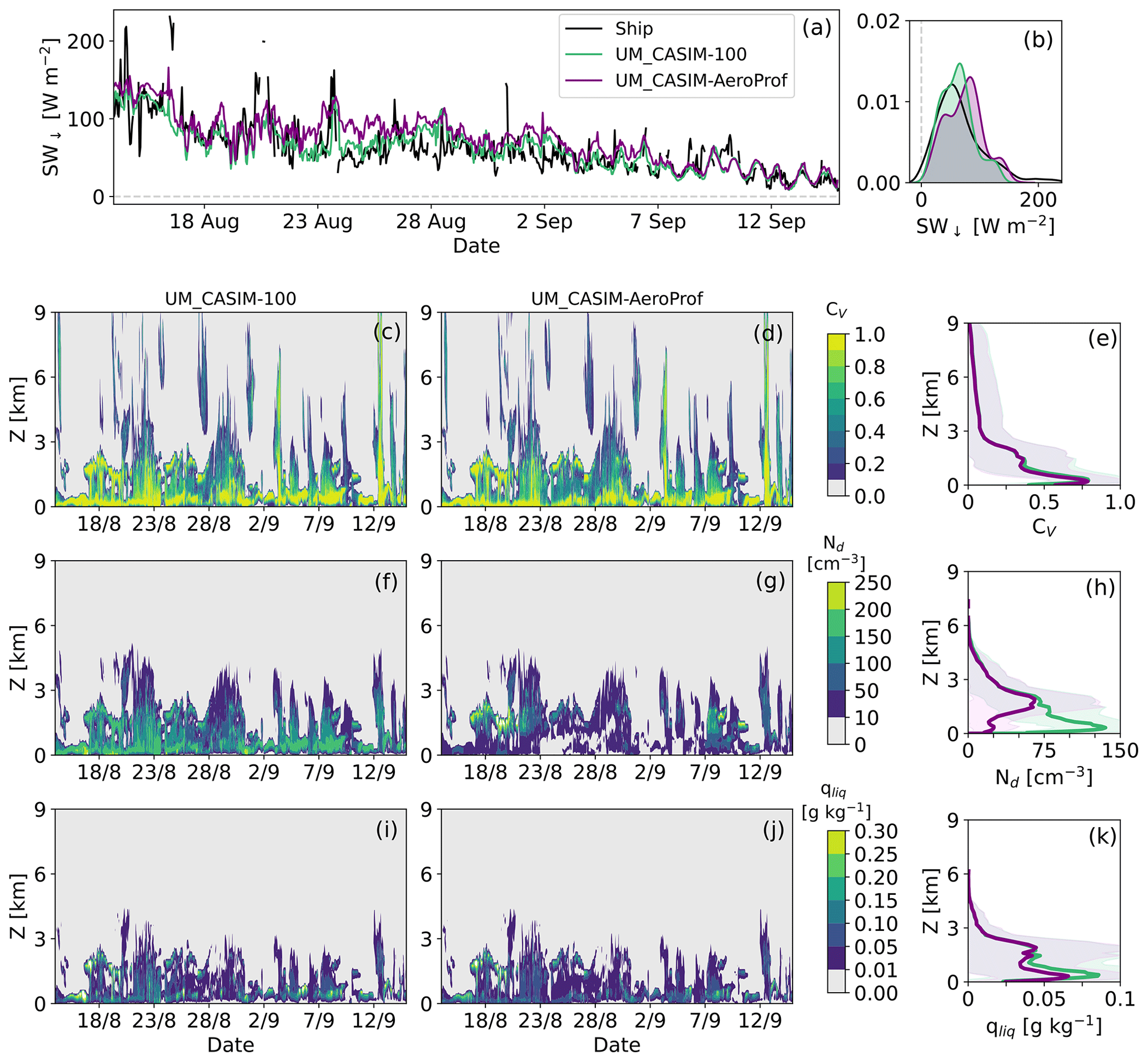
Figure 7Comparison of UM_CASIM-100 and UM_CASIM-AeroProf, demonstrating the influence of representative aerosol concentrations on the modelled cloud structure. (a–b) Downwelling shortwave radiation (SW↓) at the surface, with observations (black) shown for comparison; (c–e) CV; (f–h) cloud droplet number concentration (Nd); (i–k) liquid water mixing ratio (qliq). (c, f, i) UM_CASIM-100; (d, g, j) UM_CASIM-AeroProf; (e, h, k) mean profiles with ± 1 standard deviation shown in shading. Radiative differences are only notable between 22 and 27 August. Slight differences in qliq and cloud fraction can also be identified during this period; for example, UM_CASIM-100 produces a larger cloud fraction below 2 km on 23 August.
However, despite the differences in Nd between these two CASIM simulations, qliq does not differ much as the simulated clouds are not heavily precipitating (and thus cloud lifetime is largely unaffected). This similarity is also displayed in the diagnosed cloud fractions, related to the comparatively unaffected qliq. Despite the consistency in cloud fractions and qliq, the cloud albedo is subtly lowered (as fewer CCN are available) in UM_CASIM-AeroProf, as shown by the SW↓ comparisons in Fig. 7a–b.
3.3 Thermodynamic structure
Differences between modelled and observed cloud properties are likely related to the thermodynamic structure of the atmosphere and how well this is modelled. Figure 8 shows temperature (T) and water-vapour-specific humidity (q) from radiosondes and anomalies of each simulation with respect to these measurements. Specific humidity is considered here as a relative humidity comparison would require a calculation involving temperature: Tjernström et al. (2021) note that the errors in temperature and humidity compensate to produce a <±3 % error in relative humidity (for work with the IFS operational analyses comparing also with measurements from this campaign). This error was found to be positive below 1 km and negative around 3–5 km, and the magnitudes of these errors are within the measurement accuracy.

Figure 8T (left) and q (right) measured by the radiosondes over the AO2018 drift period. (a–b) Radiosonde data re-gridded to the UM vertical grid for model comparisons. (c–d) Biases of IFS data, re-gridded to the UM vertical grid, with respect to observations. (e–j) UM_CASIM-100, UM_RA2T, and UM_RA2M biases with no vertical re-gridding. The common vertical grid (from the UM) provides 50 vertical levels below 10 km, with 21 of these below 2 km. The black line in all the panels depicts the altitude of the main inversion base as identified using the radiosonde measurements, and meteorological time periods with common characteristics are indicated with grey-dashed lines (see Vüllers et al., 2021, for details).
Each simulation is typically too cold with respect to observations at altitudes just above the main inversion (left column; Fig. 8): this anomaly is a consistent feature throughout the drift period and across models; however, it is most prominent at the beginning of the drift. These trends indicate that the altitude of the modelled temperature inversion capping the BL is too high, likely driven by too much BL mixing and the associated too-deep cloud layers modelled in each simulation (Fig. 4b). Below the observed inversion, the simulations are typically warmer than measured; for example, on 18 August all UM simulations have a strong bias (>3 K) below the observed main inversion, with ECMWF_IFS exhibiting a similar but smaller bias. Above approximately 3 km the T biases are typically smaller in magnitude and variable in sign. All UM simulations display similar differences with respect to the radiosonde measurements; for example, each UM simulation exhibits a strong T bias up to 4.4 K at 6.5 km during 9 September.
q biases are typically small throughout much of the atmospheric column (right column; Fig. 8), with some instances of larger biases. These stronger biases are not confined to the lowest 3 km as with the temperature data. Radiosonde humidity data up to 22 August are variable aloft, and this variability affects the biases calculated over this period. However, a strong moisture bias of >0.90 g kg−1 is evident between 2 and 4 km over 20–22 August in all UM simulations. Similarly, the dry bias (of up to 1.86 g kg−1) across the UM simulations from 2 to 4 September is notable and is also present, to a lesser extent, in ECMWF_IFS (up to 0.82 g kg−1).
When these data are simplified into median profiles (Fig. 9), the characteristic biases exhibited by the models become clearer. Figure 9a, c show that the T biases are small above 4 km, with all UM simulations exhibiting a slight warm bias and ECMWF_IFS exhibiting a slight cold bias. Similarly, moisture biases are negligible above 4 km in all the simulations (Fig. 9b, d). However, below 4 km strong biases emerge.

Figure 9Median profiles of modelled (a, c) T and (b, d) q biases with respect to the radiosonde measurements over the sea ice melt (a, b) and freeze (c, d) periods (using 28 August as a threshold). Model data are coloured as previously (ECMWF_IFS: yellow; UM_CASIM-100: green; UM_RA2T: light blue; UM_RA2M: dark blue), and the ± 1 standard deviation is shown to illustrate variability. Median anomalies from the UM global model (UM_GLM; grey) are also included for reference; variability is not shown for these data.
From the surface up to 0.5 km, there is a decreasing positive T bias in all the simulations. However, the positive surface T bias is reduced during the freeze period for UM_RA2M and UM_RA2T (from +0.28/+0.31 to +0.20/+0.14 K, respectively), while it intensifies from +0.52 K (+0.46 K) to +0.90 K (+0.56 K) for ECMWF_IFS (UM_CASIM-100) (Fig. 9c).
During the melt period, all the simulations underestimate the temperature between 1 and 3 km, yet there is a clear bimodal structure evident in each profile, with secondary negative peaks at lower altitudes (Fig. 9a). ECMWF_IFS remains too cold across a deeper layer than the UM simulations, between 0.4 and 3 km. Both the IFS and the UM exhibit strong (up to −1.54 K) biases at 1.75 km. The negative T bias layers at lower altitudes differ in height between the models, with ECMWF_IFS reaching −0.94 K at 0.85 km, while the UM simulations exhibit negligible positive biases at this height. The secondary peak in the UM simulations is in fact lower in altitude, at 0.4–0.5 km. T biases are smaller than during the melt period, reaching up to −1.06 K (ECMWF_IFS) between 0.65 and 1 km, and the negative bias peak at 2 km seen previously is no longer present (Fig. 9c).
Similarly, each simulation exhibits a positive q bias towards the surface. These biases change little between the melt and freeze periods (Fig. 9b, d); ECMWF_IFS produces the greatest bias in both periods (+0.31 g m−3 during both the melt and freeze), while UM_RA2T produces the lowest bias (+0.24 and +0.10 g m−3 during the melt and freeze, respectively). ECMWF_IFS is too dry, as well as too cold, between 0.5 and 4 km, while the UM simulations are typically too moist (though variable; Fig. 9b).
There is less variability in the q biases during the freeze period. The UM simulations in particular exhibit only small q biases above 0.5 km (Fig. 9d). ECMWF_IFS performs well above 2 km; however, similarly to trends identified during the melt, it is again too dry between 0.5 and 2 km.
Figure 10 similarly shows the median T and q biases modelled by UM_CASIM-100 and UM_CASIM-AeroProf over the whole AO2018 drift period. Even though the clouds are likely more representative of the high Arctic environment in UM_CASIM-AeroProf than UM_CASIM-100, the thermodynamic biases are largely unchanged from the approximated aerosol input of UM_CASIM-100. A minor reduction in qliq between approximately 500 m and 1.5 km in UM_CASIM-AeroProf is reflected in the thermodynamic biases exhibited by these two simulations – UM_CASIM-100 has a stronger negative temperature bias at 500 m than UM_CASIM-AeroProf and a warmer BL towards the surface, likely caused by the warming effect from an overestimated cloud LWC and amount of cloud cover. We speculate that these biases would perhaps differ more so if the modelled clouds were precipitating strongly in either simulation, thus affecting qliq and cloud lifetime.

Figure 10Temperature (a) and moisture (b) biases exhibited by the UM_CASIM-100 (green) and UM_CASIM-AeroProf (purple) simulations with respect to radiosonde measurements made over the entire drift period; ± 1 standard deviation is shown in shading to illustrate variability.
However, considering each of the UM LAM configurations shown here, there is little variability in their thermodynamic biases despite the differences in their representation of aerosol inputs, cloud microphysics, and large-scale cloud schemes. Interestingly, these biases are shared by the UM global model (UM_GLM, shown in grey; Fig. 9) used to generate lateral boundary conditions for each LAM. UM_GLM exhibits similar biases to its high-resolution LAM counterparts, suggesting that these thermodynamic biases are sourced from the driving model itself.
3.3.1 Influence of the UM driving model
To investigate how the large-scale forcing is influencing the UM biases, an additional test was performed over a sub-set of the drift (31 August to 5 September) using ERA-Interim to initialise the UM global model (labelled UM_RA2M-ERAI-GLM; Fig. 11). This test was designed to evaluate whether the initial conditions of the global driving model, and therefore the associated data assimilation (DA) systems used to derive the operational analyses used for its initialisation, are responsible for the LAM thermodynamic biases we have found in this study. For this test, we used the UM_RA2M configuration for the LAM, and all global model physics options remained the same as in previous simulations (as described in Table 1); the only difference was in the initial conditions of the global model. As with the other UM LAM simulations, lateral boundary conditions are generated hourly from the global model.
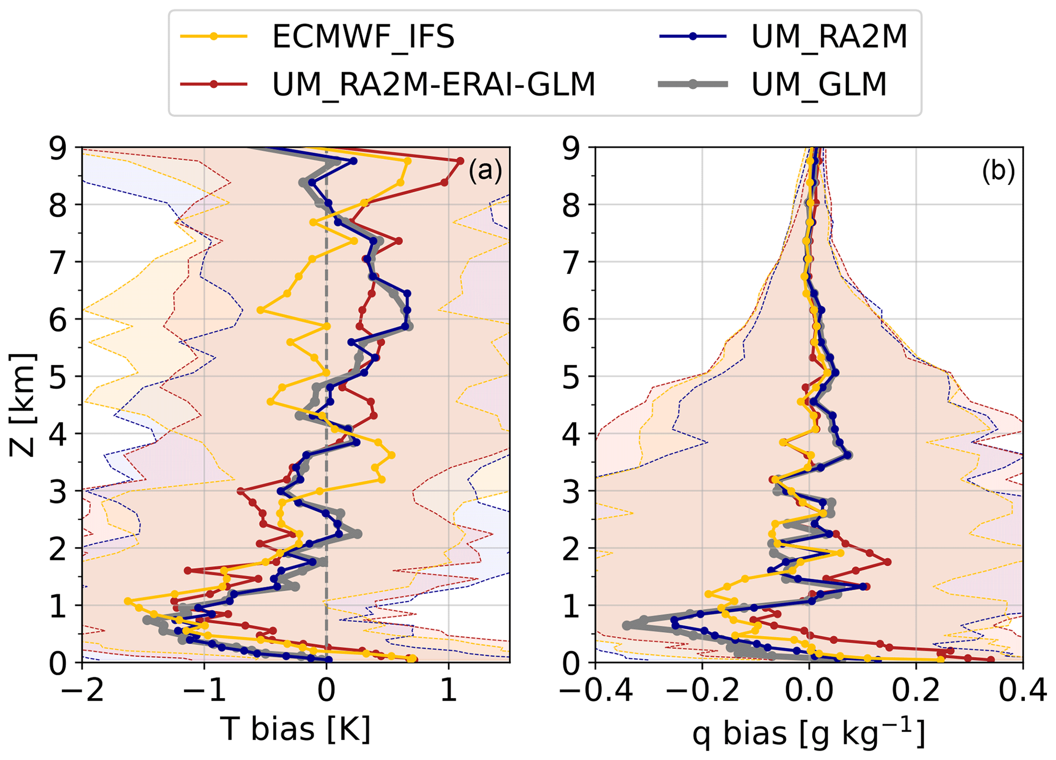
Figure 11Median T (a) and q (b) biases from a sub-set of the drift (31 August to 5 September) for ECMWF_IFS (yellow), UM_RA2M-ERAI-GLM (red), UM_RA2M (dark blue), and UM_GLM (grey). UM_RA2M-ERAI-GLM biases follow ECMWF_IFS biases up to approximately 1 km, above which they largely behave more like the other UM cases; ± 1 standard deviation is shown in shading to illustrate variability.
We find that UM_RA2M-ERAI-GLM exhibits T biases following ECMWF_IFS between the surface and 3 km, inheriting the ECMWF_IFS near-surface temperature bias discussed previously (Fig. 11a). Over this short time period, the UM simulations do not have this bias. Above 3 km, UM_RA2M-ERAI-GLM follows UM_RA2M and UM_GLM, exhibiting a slight warm bias (0.45 K at 5.5 km) in contrast to the cold bias of ECMWF_IFS (−0.65 K at the same altitude). UM_RA2M-ERAI-GLM q biases track the ECMWF_IFS biases below 1 km and between 2.5 and 9 km, with clearer alignment with UM_GLM and UM_RA2M between 1 and 1.5 km. In particular, there is a shift towards a stronger (positive) moisture bias towards the surface when the driving model is initialised with ERA-Interim.
These results confirm that the UM LAM biases within the lower atmosphere shown in Figs. 8 and 9 are driven by biases in the large-scale forcing from the global model, which is likely a combined result of the model physics and the DA used to produce the operational analyses. Given that the Arctic lacks good in situ observational data coverage, DA systems still rely heavily on their model components when creating the analysis products used for model initialisation. The comparatively comprehensive spatial coverage from satellites does not compensate for good in situ observations from radiosoundings and does little to correct a biased model DA input (Naakka et al., 2019). Therefore, improved in situ data coverage may improve these DA system biases and thus global model initial conditions. In the meantime, a different LAM configuration with a larger nested domain with lateral boundaries further from the science region of interest may break the relationship between global model and LAM biases shown here.
3.4 Links between cloud properties and thermodynamic biases
To better understand how the model thermodynamic biases relate to cloud properties in each simulation, we split our drift period further into four sub-sections – periods 3 to 6, as illustrated in Figs. 2 and 8 – to study periods of consistent meteorology. Mean equivalent potential temperature (Θe) and q profiles measured by radiosondes during these periods are shown in Fig. 12. Of the four periods considered, period 3 had cloud-free conditions most often, and the clouds which were present most typically occurred in a single layer. Periods 5 and 6 were similar; both were cloudy and influenced synoptically by three different low-pressure systems over their duration (Vüllers et al., 2021).

Figure 12Mean profiles of (a) equivalent potential temperature (θe) and (b) q measured by radiosondes launched during periods 3–6 of the expedition, with ± 1 standard deviation shown in shading.
Cloud properties and thermodynamic biases during periods 3 and 6 are shown in Fig. 13 (with similar analyses for periods 4 and 5 included as Fig. S7). As mentioned previously, mean observed cloud occurrence was lower for period 3 than in any other period during the drift. All the simulations overestimate the TWC cloud mask below 2 km, with each UM case producing a bimodal mean profile peaking below 0.5 and at 1.8 km (Fig. 13a). Such bimodality is less clear with ECMWF_IFS: it exhibits a lower layer with the cloud top at 1 km and a more prominent secondary layer at 1.6 km, although the separation of these layers is not as distinct as in the UM cases. The secondary layer at 1.6 km has a greater LWC than the lower layer, with a peak of 0.14 g m−3 (Fig. 13b). The bimodal cloud structure is also liquid-dominated in the UM simulations, where both peaks reach around 0.1 g m−3 (and even exceed this magnitude in the 1.8 km layer), across all three configurations.
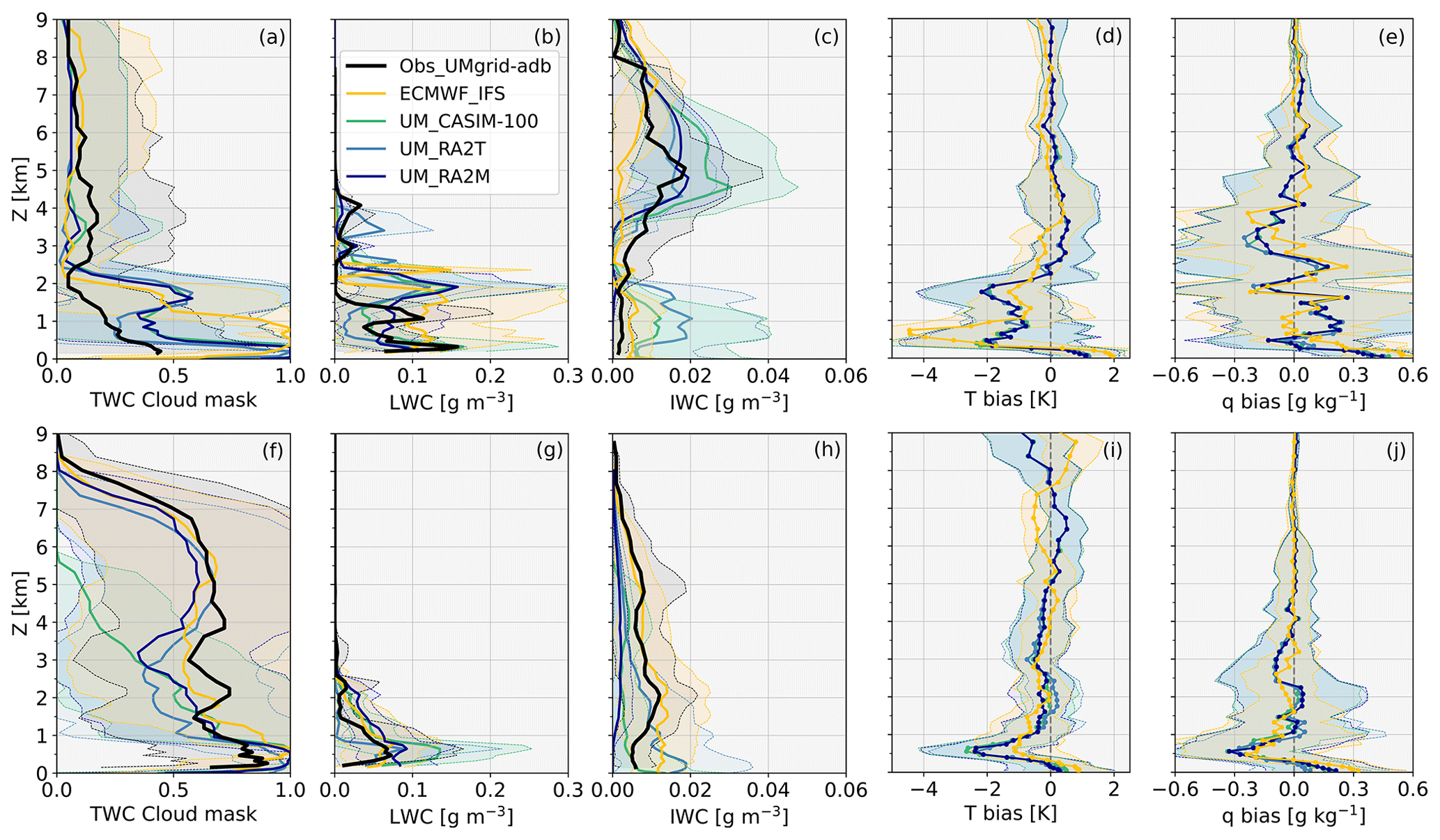
Figure 13Comparison of mean cloud mask, LWC, and IWC profiles with median biases in T and q with respect to radiosondes for period 3 (a–e, top row) and period 6 (f–j, bottom row). Again, observed LWC was calculated assuming adiabatic conditions using Cloudnet; ± 1 standard deviation is shown in shading to illustrate variability.
Considering the corresponding median T biases (Fig. 13d), there are clear correlations between negative biases and modelled cloud height, suggesting that cloud-top longwave cooling is a contributing source of these biases. The lower-layer (0.75 km) bias in ECMWF_IFS is particularly striking, reaching −4.45 K, and corresponds to the top of a large fraction of liquid-dominated cloud (Fig. 13a, b). The mean LWC modelled at this altitude is over 3 times greater than was observed, with cloud frequency overestimated by 73 %. q biases (Fig. 13e) are negligible for ECMWF_IFS between 0.75 and 1 km yet positive below and above this altitude range. The coinciding overestimation of cloud at these heights indicates that the IFS has simulated too much condensation, driven by the availability of too much moisture. Similarly, all the UM simulations exhibit a moist bias between 0.5 and 1.6 km between the modelled cloud layers and exhibit small dry biases where too much cloud is modelled (e.g. 0.5 km). These results indicate that both models have an excess of water vapour, particularly below 3 km, where negligible/dry biases with comparison to observations are in fact an artefact of too much condensation and the resulting cloud cover. This excessive cloud cover, on the other hand, has a negative effect on the temperature bias profile, resulting in strong cold biases.
The models are in good agreement with the observed LWC during period 6, with the exception of UM_CASIM-100, which produces double the observed LWC at 0.7 km (Fig. 13g). In particular, ECMWF_IFS performs well below 2.5 km in terms of LWC, IWC, and cloud occurrence, with the largest difference in the latter occurring at approximately 0.7 km (100 % in ECMWF_IFS in comparison to the 79 % observed). Consequently, the T biases are smaller during period 6 than period 3 for ECMWF_IFS. However, these T biases are still present (Fig. 13i), peaking at −0.96 K at 0.65 km, likely caused by this minor overestimation in cloud cover, albeit with representative microphysics.
The magnitude of the T biases for the UM simulations is similar between both periods, likely caused by this model producing up to 100 % cloud cover at low altitude. All the UM simulations exhibit stronger T and q biases below 1 km than ECMWF_IFS during period 6 (Fig. 13i–j). Strong negative T biases accompany the overestimation of cloud cover in each UM case, and the improved model–observation agreement of LWC by UM_RA2M and UM_RA2T does little to alleviate these biases with comparison to the overestimated LWC of UM_CASIM-100. Simply, there is too much low-altitude (below 1 km) cloud causing too much cloud-top radiative cooling in the model, no matter which representation of cloud microphysics or large-scale cloud is used.
However, while the q biases were negligible when ECMWF_IFS exhibited particularly strong T biases during period 3, q biases for the UM become notably negative for the similarly strong cold bias during period 6; this is the largest dry bias simulated over the four periods considered (with periods 4 and 5 included in the Supplement). The surface q bias for the UM simulations is smaller during period 6 than during period 3, and the tropospheric q bias is positive less often, suggesting that the positive moisture bias hypothesised previously (leading to too much condensation and cloud cover) is not ubiquitous in the model. In fact, results shown in Fig. 13 and Fig. S7 for periods 4 and 5 suggest that either the increased synoptic activity or freezing sea ice conditions (or both) of periods 5 and 6 act to reduce this moist bias in the UM.
In summary, both models exhibit strong negative T biases at altitudes coinciding with too much liquid-dominated cloud (e.g. Fig. 13a, b, d), likely caused by the consequent enhancement of cloud-top radiative cooling and subsequent feedback on low-altitude cloudiness. q biases improve where cloud is modelled during the melt period (Fig. 13a, e), suggesting that the q field was perhaps too moist below 3 km to begin with, leading to too much condensation and excessive cloud cover. However, this hypothesis does not appear to be valid during the freeze or at altitude, as indicated by the negative q biases above 2.5 km which occur where more cloud was observed than modelled, e.g. 2.5 to 4 km during period 3 for all the simulations (Fig. 13a, e) or 2.5 to 3.5 km for the UM simulations during period 6 (Fig. 13f, j). In these instances, our models produce too little cloud as they are too dry to facilitate cloud formation. With underestimated cloud formation, the models are also slightly too warm (approximately 0.3 K) due to the missing radiative cooling occurring at these altitudes in reality.
While the model T biases align well with their overestimation of cloud cover, our analysis thus far does not account for the height of the capping inversion. Therefore, incorrect placement of cloud in the models or a too-deep or too-shallow modelled BL could be contributing to these biases and thus could affect the interpretation of our results.
Figure 14 shows the strongest temperature inversion base identified from each model simulation and the radiosonde measurements. In each dataset, the strongest inversion below 3 km was identified (following Vüllers et al., 2021); if a weaker inversion was modelled at a lower altitude which was closer to the inversion base identified from the radiosonde, the model inversion height was adjusted accordingly. In keeping with previous analysis, radiosonde and IFS data were interpolated to the UM vertical grid for fair comparison; this procedure smooths some high-altitude detail in the radiosonde profiles, such that the strength of some higher-altitude inversions is reduced, causing weaker low-altitude inversions to be identified as the primary inversion instead.

Figure 14Model temperature inversion base as a function of the identified inversion base from radiosonde (RS) measurements. org. inv: strongest inversion below 3 km, identified following Vüllers et al. (2021). adj. inv: where models exhibit a secondary weaker inversion at lower altitude, in better agreement with identified radiosonde inversions, these identified inversions are adjusted accordingly. unadj.inv: unadjusted primary inversions, not used for further analysis and shown for reference only. Correlation coefficients for the combined adj. inv plus org. inv data are shown in red at the top of each panel.
These results indicate that the strongest (unadjusted) inversion in each simulation is often too high (grey points, Fig. 14), and weaker inversions at lower altitude are typically in better agreement with identified inversions from radiosondes. Low inversion bases (below approximately 0.5 km) are consistently overestimated in each simulation, particularly during the melt period (not shown), supporting our previous deduction that the model inversions were often too high. The detection algorithm does fail to capture some inversions, predominantly during the freeze period, and instead underestimates the modelled inversion base during this time window with comparison to measurements (lower right-hand points in each panel).
Modelled and observed temperature profiles were scaled using these identified inversions to remove the differences in inversion height from our interpretation of the model biases (Fig. 15). When averaged over the full drift, the models are largely biased warm below the inversion and cold above (up to 3 km; Fig. 15a), with the exception of UM_CASIM-100, which also exhibits a subtle cold bias just below the inversion. This warm-below/cold-above signal is more consistent between the models during the melt period (Fig. 15b). Above the inversion, ECMWF_IFS exhibits a stronger cold bias than the UM simulations. The shape of the scaled profile is rather consistent between the melt and freeze with ECMWF_IFS; the model is consistently too warm below the inversion and too cold above, with comparison to radiosonde measurements. However, the UM simulations, particularly UM_RA2M, are partially biased cold below the inversion during the freeze. As previously mentioned, biases during the freeze period must be interpreted with caution as the inversion detection algorithm performed less well during this time window, with several modelled inversions missed. However, these scaled T bias profiles support our previous hypothesis that cloud longwave cooling is producing colder thermodynamic conditions in the models than were observed, irrespective of the differences between modelled and observed inversion heights. Similarly, the warm surface bias indicated previously can be interpreted as spanning most of the lower troposphere below the main inversion base rather than solely near the surface.

Figure 15Scaled median model–observation T bias profiles for the full drift (a), melt (b), and freeze (c) periods. Profiles are scaled such that −1 is the surface, 0 is the main inversion base, and 1 is 3 km.
4.1 Surface radiative balance
4.1.1 Shortwave
The small SW↓ biases exhibited by the standard UM configurations concurrent with a more significant SWnet bias indicate that the modelled surface albedo is too low. While the observed albedo may be biased high due to its calculation from a spatially small sample of sea ice (directly surrounding the ship), the UM surface albedo parameterisation has previously been shown to be too low in the high Arctic (Birch et al., 2009, 2012). The temperature and albedo limits used in the standard Regional Atmosphere parameterisation have been increased since Birch et al. (2009, 2012); however, Fig. 2 demonstrates that the snow-on-sea-ice parameterisation limits tested here with ECMWF_IFS and UM_CASIM-100 produce a better comparison with our high Arctic measurements.
4.1.2 Longwave
The root of the longwave error in each simulation is likely the >90 % liquid-dominated low-cloud occurrence, which is not representative of the observations (Fig. 4b). This problem has been previously identified in the high Arctic with both models used in this study (Birch et al., 2012; Sotiropoulou et al., 2016), and recent model improvements/microphysical changes have not sufficiently improved model performance in this regard. The positive longwave biases are consistent with the too-warm surface T biases in all the simulations (Figs. 9, 10), which is also consistent with previous findings with both models (Birch et al., 2009; Sotiropoulou et al., 2016) and with the ERA-Interim reanalysis product (Jakobson et al., 2012; Wesslén et al., 2014). Figures 9 and 10 suggest that the UM simulations are perhaps better at capturing the near-surface T over the freeze, while ECMWF_IFS consistently has a warm surface bias regardless of season. The overestimation of cloud cover and LWC, which drives too much radiative cooling at the cloud top, will contribute an excess LW↓ flux which would act to warm the lower BL and thus contribute this warm bias. Tjernström et al. (2021) suggest that the surface is warmed by the atmosphere in the IFS, not the opposite, as indicated by the enhanced downward sensible heat flux in combination with diminished SW↓ with comparison to observations.
Given these results, we suggest that excessive cloudiness is likely a contributing factor to the warm surface bias in all the simulations. In particular, it is noteworthy that UM_CASIM-100 performs the most poorly of the UM simulations. This result is disappointing given the improvement of UM_CASIM-100 over the standard Regional Atmosphere configurations in both SW↓ and SWnet. Including CASIM aerosol processing through wet scavenging – thus enabling cloud dissipation (e.g. Stevens et al., 2017) – may rectify this issue or the representation of prognostic ice-nucleating particles (INPs) in place of a simple diagnostic relationship between temperature and cloud ice number concentrations (e.g. Varma et al., 2021). These pathways will be explored in future work; however, it is highly likely that other meteorological factors (e.g. mean sea level pressure anomalies and the subsequent influence on cloud dynamics) and incorrect model processes (e.g. turbulent flux biases) are contributing to this warm surface bias across all our simulations, in addition to cloudiness (Tjernström et al., 2021).
4.2 Lower troposphere
4.2.1 Temperature
Temperature biases are strongest within the lowest 3 km of our model domains (Figs. 9, 13); this is also the altitude range over which the models overestimate cloud occurrence. With too much cloud, cloud-top radiative cooling likely lowers the temperature too efficiently; this, coupled with incorrect cloud positioning (e.g. period 3; Fig. 13), gives a cold bias above the observed main capping inversion. Where the liquid (and ice) phase is modelled more effectively – e.g. ECMWF_IFS during period 6 (Fig. 13) – the associated median biases are smaller (<±1 K), supporting this conclusion. Turner et al. (2018) note that the presence of cloud aloft can significantly modulate the radiative cooling response of low-level Arctic clouds – in period 6, multi-layered clouds were prevalent, thereby potentially muting the radiative impact. In period 3, however, few clouds were observed, and those which were present often occurred in single layers (Vüllers et al., 2021); during this period, we found the greatest thermodynamic biases in our models with respect to our observations.
The dipole in T errors shown in Figs. 8 and 9, with a positive bias towards the surface below a negative bias between 0.5 and 3 km, suggests that heat and moisture are not being sufficiently transported upwards from the surface or downwards from cooling at the cloud top. This T bias is present in all the simulations during both the melt and freeze periods and could result from the models failing to reproduce the structure of more than one strong observed inversion, instead exhibiting comparatively smooth T profiles. As shown by Fig. 14, the heights of low-altitude T inversions are often overestimated by the models, particularly during the melt period (not shown): this too-deep surface mixed layer likely results in incorrect cloud placement, leading to thermodynamic model–observation biases on a 1 : 1 comparison. Our scaled thermodynamic analysis (Figs. 14, 15) indicates that, while the models are often incorrectly placing the temperature inversion (consistent with previous findings; Birch et al., 2012), the relationship between too much cloud and strong negative T biases suggested by Fig. 13 appears to be robust under these scaled height adjustments by the inversion base and that the simulations are still largely too warm below the inversion.
Both Sotiropoulou et al. (2016) and Tjernström et al. (2021) found a similar vertical structure of the temperature biases with the IFS model, with positive biases within the lower 0.5 km of the atmosphere and a consistent cold bias present around 1 km. Tjernström et al. (2021) found that this cold bias intensifies with time during 3 d forecasts, indicating that it is made worse by processes within the model. They hypothesised that the mid-level convection parameterisation triggering too efficiently within the IFS could be transporting water vapour out of the BL, resulting in too much condensation to form cloud. While our UM LAM simulations do not employ such a convection scheme, the global driving model does. Given the apparent close relationship between the biases exhibited by the LAM and the global model (Figs. 9, 11), we conducted a short 6 d test with the global mid-level convection scheme switched off; this test caused over an order of magnitude increase in the UM_GLM cold biases shown in Fig. 11 (not shown). More investigation into vertical transport and mixing of scalars (temperature, moisture, and clouds) is needed; however, such an investigation is beyond the scope of this paper.
4.2.2 Moisture
During the melt period, our results indicate that the UM is particularly moist throughout much of the troposphere (Fig. 9b), suggesting that the melting ice is enabling a too-great moisture source from the surface to the atmosphere. However, this tropospheric bias appears to be rectified during the freeze, while the surface bias remains (Fig. 9d); therefore, the hypothesised melting ice source is likely not the only contributor to this moisture bias. Latent heat fluxes measured during the expedition indicate no significant change between the melt and freeze periods (not shown); therefore, the hypothesised increased moisture flux during the melt is unlikely.
Given the close relationship between our UM LAM and global model biases (Figs. 9, 11), increased poleward moisture transport introduced at the lateral boundary conditions from the mid-latitudes could partly explain these biases. This phenomenon has been previously identified as a consequence of climate change and may promote increased cloudiness in the polar regions (e.g. Held and Soden, 2006; Vavrus et al., 2009; Allen et al., 2012; Bender et al., 2012). The moist surface bias is also present over both the melt and freeze in ECMWF_IFS; however, ECMWF_IFS is routinely too dry between 0.5 and 4 km, in contrast to the UM. Instead, the IFS traps too much moisture in the lowest 0.5 km, suggesting that the upward transport of moisture may be insufficient, the cloud sink above 0.5 km is too great, or there are consistent biases introduced via assimilation of data other than the radiosonde data (e.g. satellite).
The moist bias exhibited by ECMWF_IFS towards the surface has previously been highlighted by Sotiropoulou et al. (2016), who suggested that this problem may explain why this model struggles to reproduce humidity inversions above the BL. There are instances where negative T biases coincide with negative q biases at altitudes just above the main temperature inversion (for example, on 27 August; Fig. 9). Moisture inversions have often been observed during the Arctic summertime (Sedlar et al., 2012; Nygård et al., 2014). ECMWF_IFS fails to reproduce such inversions observed during AO2018. This dry bias above the observed capping inversion around 27 August is not as strong in the UM simulations, but the UM does successfully reproduce a small humidity inversion.
4.3 Cloud macrophysics and microphysics
The UM simulations have >98 % cloud occurrence around 0.2 km over all four periods. Reduced SW↓ biases with respect to the standard Regional Atmosphere configurations indicate that UM_CASIM-100 does improve agreement with our high Arctic observations (Table 3), though there are still clear deficiencies in model capability.
The ice phase differs more between the models than the liquid phase, likely due to its strong relationship with temperature: UM_RA2M and UM_RA2T use the Fletcher (1962) parameterisation for primary ice formation, while ECMWF_IFS uses Meyers et al. (1992) and UM_CASIM-100 uses Cooper (1986). Each of these parameterisations is inherently temperature-dependent, with Meyers et al. (1992) producing the largest ice number concentration and Fletcher (1962) producing the smallest. Given that each simulation does not reproduce the observed temperature profile well below 3 km, the onset of ice nucleation (occurring below a threshold of −10 ∘C in the UM, for example) will be affected. If ice production is triggered prematurely, cloud liquid properties should be dampened via the Wegener–Bergeron–Findeisen mechanism; evidence of this can be seen in UM_RA2T during period 3, where an overestimation of ice below 2 km corresponds to a smaller mean LWC than the other simulations (Fig. 13b–c).
When considering the drift as a whole, IWC is overestimated by all the simulations (except UM_RA2M) below 1.5 km, where our T and q biases are at their greatest. To test whether the method of parameterising primary ice itself has any effect on these biases, we used the Fletcher (1962), Cooper (1986), and Meyers et al. (1992) parameterisations over a short test period within the CASIM framework; however, we found little difference in the tropospheric ice with the different parameterisation methods (Fig. S8). Given the spread in IWC results shown here, further investigation into the best methods to represent primary ice production in such global and NWP models should be considered in future, with specific focus on employing prognostic ice-nucleating particles or a diagnostic temperature-dependent function based on Arctic measurements (Li et al., 2022) to facilitate ice formation.
Below 3 km, the mean modelled LWC often exceeds the observed value (Figs. 4, 13). This overestimation of cloud liquid is also evident from the LWP data, with each simulation exhibiting a greater LWP than was measured (Fig. 5) when averaged over each period (not shown). The exception to this is UM_RA2T; this is the only simulation which often underestimates LWP, due to its increased cloud ice mass within the lower troposphere in comparison to the other simulations (Fig. 4d). The mean measured LWP during period 3 is 122.8 g m−2, yet UM_RA2T only produces 70.4 g m−2. In contrast, UM_RA2T reproduces the mean measured LWP well during period 6 (48.5 g m−2 measured versus 43.2 g m−2 modelled), with agreement improving with time throughout the drift. This efficient ice-producing simulation suggests that the ice phase influences cloud properties as time progresses more so in reality, while the other UM cases, with less-dominant ice microphysics, retain too much liquid in comparison to the measurements. To an extent, ECMWF_IFS also behaves in this way, retaining too much cloud liquid; however, it performs much better than UM_RA2M and UM_CASIM-100 in reproducing the mean LWC and IWC during period 6 (Fig. 13g, h).
These simulations suggest that the model development community has effectively reduced the ice-phase efficiency too much in central Arctic mixed-phase clouds. The surface longwave balance is positively biased, and these excessive low-level clouds are a contributing factor: by enabling too much liquid to form, these clouds efficiently absorb and re-emit upwelling longwave radiation back towards the surface. Our results show that we have made great improvements in the shortwave, driven by the improvements we have made to our cloud physics representation in these models (in addition to a better estimation of the surface albedo). However, the too-consistent cloud cover coupled with too much cloud liquid is hampering our model capability, and further developments (such as the inclusion of representative CCN and INP inputs in double-moment cloud schemes to facilitate cloud dissipation) will likely go some way to tackling this issue.
Met Office UM and ECMWF IFS model performance was evaluated using observations made in the high Arctic during the Arctic Ocean 2018 expedition, with particular focus on modelled clouds and the surface radiative balance. Four key simulations were considered: a global configuration with the IFS and three nested configurations with the UM (each using different combinations of large-scale cloud and microphysics schemes but driven by the same global model set-up). These four simulations were compared with observations by using Cloudnet to build model-comparable cloud fractions and water contents and thus to identify consistent model weaknesses between the configurations chosen.
Modelled BLs are often too deep (Fig. 9, 14), particularly during the melt period, and thermodynamic biases, cloud occurrence, and cloud microphysics are consequently in poor agreement with observations below 3 km. Excessive low-cloud occurrence is prevalent in both models (Fig. 3), and no simulation adequately reproduced cloud-free periods and the associated increases in longwave net emission (Fig. 2). Strong negative temperature biases (Figs. 8, 9, 13) coincide with too-frequent liquid-dominated cloud layers (Fig. 13a, b, f, g), likely associated with overproductive cloud-top radiative cooling and subsequent feedbacks on low-level cloudiness in the models. Cloud liquid and ice water contents, especially below 1 km, were within an order of magnitude of the observations (Fig. 4), but clouds occurred too frequently, contained too much liquid between 1 and 3 km, and were often at too high an altitude (Fig. 13a–c).
Radiative interactions are in better agreement with observations, and all the models capture the observed distribution of SWnet and LWnet better during the sea ice freeze period in comparison to the melt period (Fig. 9). Improved radiative interactions and thermodynamic biases during the freeze can be linked with improved agreement of cloud occurrence and microphysics (Figs. 13, S7). The surface albedo in each model configuration is underestimated with respect to observational estimates (see Supplement), but this is unsurprising given that the models are representing an average albedo over a km grid box, while our observed estimates are from the area immediately surrounding the ship. Updating the surface albedo parameterisation limits used within the UM Regional Atmosphere configurations (UM_RA2M/UM_RA2T) to those used in the Global Atmosphere GA6.0/6.1 configuration (UM_CASIM-100) greatly improves our surface albedo comparison with observational estimates (see Supplement) and thus contributes to the good comparison of UM_CASIM-100 with measured shortwave radiation data.
We propose that four factors are important to failings in our model simulations.
-
The choice and use of large-scale cloud schemes at high resolution
Both the UM and IFS poorly capture Cloudnet-calculated cloud fractions from observations over August–September 2018 in the central Arctic, particularly at altitudes between 2 and 8 km (Fig. 4a). Building a comparable mask based on TWC shows that the cloud modelled aloft is actually in good agreement with observations (Fig. 4b) while highlighting that the overprediction of cloud occurrence below 3 km is in fact much worse than suggested by the CV comparison. As such, we suggest that cloud fractions should not be used in isolation as a model comparison metric over the Arctic, as models represent this parameter differently at the present time (as detailed in the Supplement), and we would advocate for the use of cloud water contents to derive comparable cloud occurrence metrics between observations and models.
-
The cloud microphysics scheme chosen to represent resolved clouds
UM_CASIM-100 performs best in terms of SWnet (Fig. 2, Table 3), but it struggles to capture cloud-free episodes, thus producing a LWnet PDF which is too narrow in comparison to our measurements. ECMWF_IFS shares the too-narrow LWnet PDF of UM_CASIM-100; however, it often produces a IWC in reasonable agreement with observations, and its mean LWC profile does agree particularly well with the observations at times (e.g. period 6; Fig. 13g). Of the UM simulations considered, UM_CASIM-100 is in best agreement with both ECMWF_IFS and observations in terms of net radiation, SWnet, and SW↓. This improved radiative agreement can be linked to its better cloud microphysical agreement with our Cloudnet-derived cloud liquid water content over the standard Regional Atmosphere configurations (Figs. 4, 5, 13); however, UM_CASIM-100 produces even poorer cloud fractions aloft than either UM_RA2M or UM_RA2T.
-
Representative CCN concentrations, and thus droplet number concentrations, as a function of altitude
Representative CCN concentrations in UM_CASIM-AeroProf somewhat improve the overestimation of qliq within low-level clouds in UM_CASIM-100. However, the qliq decrease is not sufficient to trigger an increase in liquid precipitation, which would thus decrease cloud lifetime, and so the modelled CV is essentially unchanged (Fig. 7). Crucially, thermodynamic biases with respect to observations are not improved through this enhanced complexity (Fig. 10), highlighting that these biases may not be fixed by a more comprehensive representation of cloud physics. Further work is required, with the inclusion of wet scavenging of aerosols and prognostic INPs, to rule out whether such processes could improve the model biases over and above the inclusion of representative aerosol concentrations alone.
-
The global model analyses used to produce boundary conditions for high-resolution nests
The thermodynamic biases identified in our models differ only a little between the UM simulations despite differences in their cloud configurations. Comparisons with the global model show that the biases within the LAM are largely inherited from the global model and its initial conditions (Figs. 9, 11); therefore, for LAM configurations such as that tested here, we will not obtain the true benefit of more sophisticated cloud microphysics schemes in NWP simulations until we address the large-scale biases in their driving models/DA system.
While representative CCN concentrations are indeed important for properly reproducing Arctic cloud structure and its consequential impact on the net surface radiation, our findings indicate that such representative cloud nuclei inputs still have only a small impact on thermodynamic biases in the lower troposphere. For our given LAM configuration, we speculate that these biases will always be inherited from the driving model/DA and will continually bias cloud formation processes and BL depth; however, using an increased domain size, with the science area of interest as far from the lateral boundaries as possible, may help to reduce the influence of the driving model/DA. The issue of inherited thermodynamic biases is concerning as both the UM global model and IFS are both used within the community to drive NWP configurations of the same model (UM) or others (IFS). For example, the IFS configuration tested here is similar to that used by ERA5; therefore, these biases could influence future high Arctic NWP simulations if these reanalyses are used for initialisation.
Our recommendations are thus twofold. To improve our Arctic cloud modelling capability, we must continue to improve the cloud physics description, striving for an optimum complexity, such as the introduction of representative CCN concentrations and double-moment cloud liquid illustrated here in addition to the inclusion of prognostic INP and associated aerosol processing mechanisms. However, we must concurrently address the overabundant occurrence of a too-well-mixed and too-cloudy lower troposphere and tackle the resultant thermodynamic biases in our global driving models and their respective DA systems.
LWP measurements from the HATPRO microwave radiometer were used in this study; this instrument provides measurements of microwave brightness temperatures, from which LWP is derived for the full atmospheric column above the instrument (here located approximately 13 m above the surface). This includes measurement of liquid clouds at altitudes below the radar's first range gate at 156 m. Fog periods occurred frequently throughout the expedition (Vüllers et al., 2021); therefore, we had several instances where liquid fog was measured with HATPRO with small quantities of liquid, or none, detected in the clouds above (from lidar/radar).
Cloudnet calculates an offset to be deducted from the LWP time series dependent upon its categorisations of cloud to ensure that liquid is partitioned throughout the cloud column only if liquid clouds were present. This offset is non-uniform, calculated as a given fraction of the LWP signal on a daily basis, and is deducted from the LWP data to ensure liquid partitioning is conducted correctly within the Cloudnet algorithm. Given the frequency of fog occurrence, this offset was often overestimated and too much liquid data were removed, thus negatively impacting the LWP and LWC comparisons with our model simulations.
To rectify this problem, we removed the LWP offset calculation from the Cloudnet procedure, enabling all ingested data to be used by Cloudnet. We then compared these adapted Cloudnet LWC data to a LWC calculated under an adiabatic assumption to test whether the latter could be used as an approximation of the true LWC if there was not as much fog present during the expedition. Figure A1 shows this comparison using all data from the drift period and indicates that, by keeping all fog liquid data in the time series, Cloudnet artificially partitions these data to liquid cloud layers identified by the lidar, leading to too much liquid in clouds within the lowest 1 km of the atmosphere (with comparison to the adiabatic profile). These data also indicate that we can safely use the adiabatic LWC as this artificial liquid enhancement is confined to the lowest 1 km and does not significantly affect the comparison for higher altitudes. Following these comparisons, we chose to include the adiabatic LWC in our comparisons with model simulations to exclude the artificial enhancement of cloud liquid at low altitudes in our measurement data. However, it must be noted that it is unlikely that these clouds are truly adiabatic, and therefore we are potentially overestimating the observed cloud liquid water content in this study.
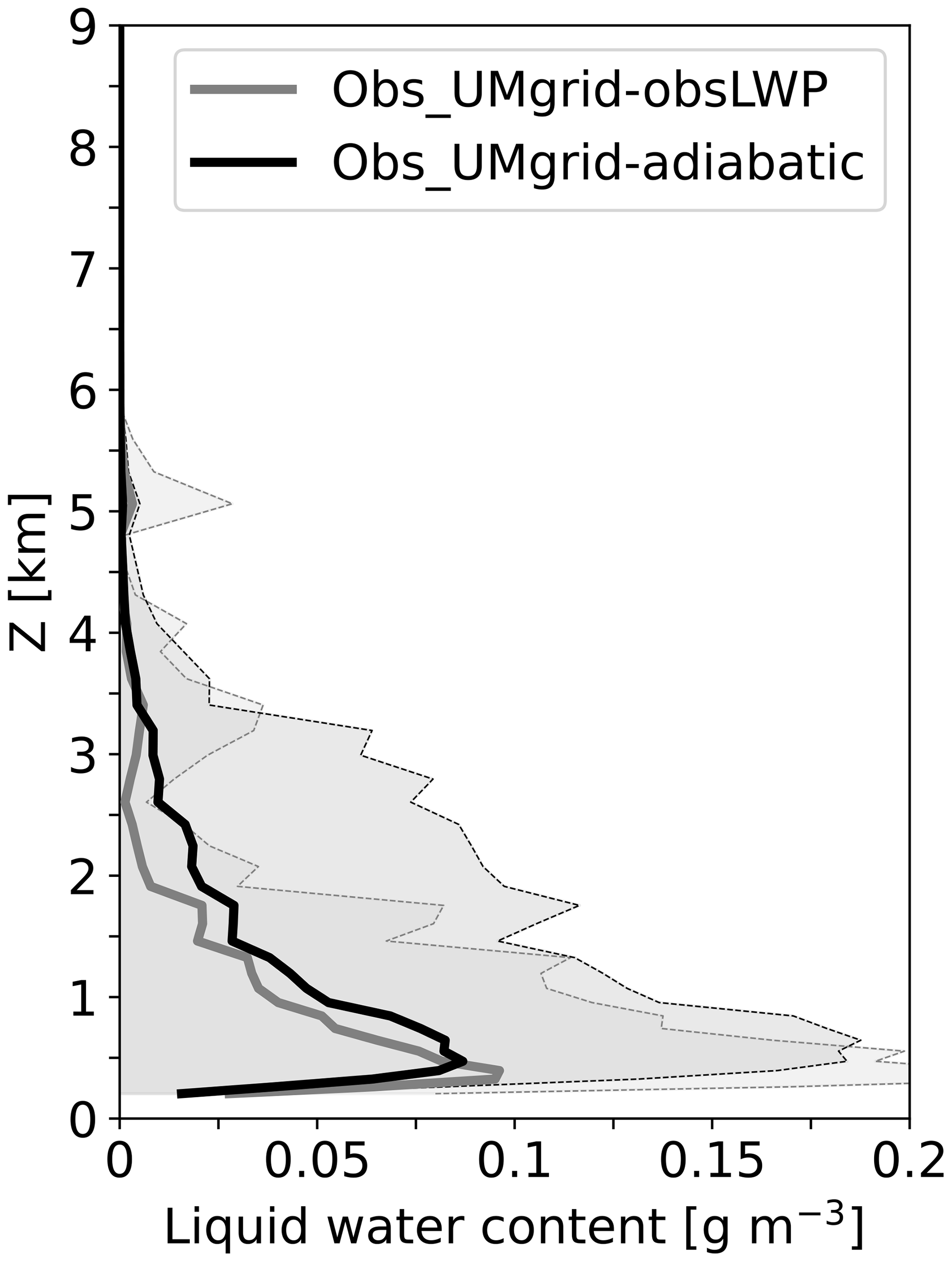
Figure A1Comparison of mean LWC profiles calculated using an adiabatic assumption (black, ± 1 standard deviation shown in dark-grey shading) and from HATPRO LWP measurements (grey, ± 1 standard deviation shown in light grey) without the Cloudnet offsetting procedure.
UK contributions, as well as selected other data, are available within the MOCCHA (Microbiology-Ocean-Cloud Coupling in the High Arctic) data collection in the Centre for Environmental Data Analysis (CEDA) archives (http://catalogue.ceda.ac.uk/uuid/7f35130cb8c947bf9013594aec6b3043, Brooks et al., 2020). Cloudnet data associated with the ECMWF_IFS simulation are stored at https://doi.org/10.5285/4c0e990d61454c22be9030777c7fbe89 (McCusker and Vuellers, 2023a), in addition to the compiled raw model data and Cloudnet data for UM_RA2M (https://doi.org/10.5285/31a23a7fbb2c40828e8af2fd479b683e, McCusker and Vuellers, 2023b), UM_RA2T (https://doi.org/10.5285/180f1c51a22f4fc48c947d33f6c0815e, McCusker and Vuellers, 2023c), and UM_CASIM-100 (https://doi.org/10.5285/ebc32b4b3e3d4e1788bbdd66b6abb5de, McCusker and Vuellers, 2023d). Other cruise data are available from the Bolin Centre for Climate Research MOCCHA/AO2018 holdings (http://bolin.su.se/data, last access: 4 January 2021), including the ship navigation data (https://catalogue.ceda.ac.uk/uuid/9405b2f8056947609da4bcc0bc88c5e8, Brooks and Vüllers, 2020), Cloudnet data (https://doi.org/10.17043/ao2018-cloudnet-3; Vüllers et al., 2020), radiosonde data (https://doi.org/10.17043/ao2018-radiosonde-2; Prytherch et al., 2019), present weather sensor data (https://doi.org/10.17043/ao2018-present-weather; Prytherch, 2019), weather station data (https://doi.org/10.17043/ao2018-misu-weather-2; Prytherch, 2020), surface meteorological data from the on-ice installations (https://catalogue.ceda.ac.uk/uuid/bac887be794d4c4587f302f764c12ec4, Vüllers and Brooks, 2021), and micrometeorological data (https://doi.org/10.17043/ao2018-micromet-oden-3; Prytherch and Tjernström, 2020).
The supplement related to this article is available online at: https://doi.org/10.5194/acp-23-4819-2023-supplement.
GYM led the model data analysis, aided by PF, RP, JJD, and RF. JV led the measurement and Cloudnet data analysis, with contributions from PA, IMB, MT, and EO'C. IMB, PA, MT, and JP performed the measurements during AO2018. IMB, MT, JJD, PF, RN, GYM, and JV all contributed to the study design. All the authors contributed to the discussion of the results and the writing of the manuscript.
The contact author has declared that none of the authors has any competing interests.
Publisher’s note: Copernicus Publications remains neutral with regard to jurisdictional claims in published maps and institutional affiliations.
This work was supported by the UK Natural Environment Research Council (NERC; grant no. NE/R009686/1) and the Knut and Alice Wallenberg Foundation (grant no. 2016-0024). Jonathan J. Day was supported by European Union project INTERACT 3 (GA 871120). The Swedish Polar Research Secretariat (SPRS) provided access to the icebreaker Oden and logistical support. We are grateful to the chief scientists Caroline Leck and Patricia Matrai for planning and coordination of AO2018, to the SPRS logistical staff, and to the icebreaker Oden's captain Mattias Peterson and his crew.
The Atmospheric Measurements and Observations Facility (AMOF) of the UK National Centre for Atmospheric Science (NCAS) provided the cloud radar, HALO lidar, RPG HATPRO radiometer, Campbell ceilometer, Kipp & Zonen radiometers, and Vaisala radiosounding station. The soundings were supported by Environment and Climate Change Canada in collaboration with the Year of Polar Prediction, Polar Prediction Project.
We made use of the Monsoon2 system, a collaborative facility supplied under the Joint Weather and Climate Research Programme, a strategic partnership between the Met Office and the Natural Environment Research Council. This work also used JASMIN, the UK collaborative data analysis facility, and was achieved in part with help from the Centre for Environmental Modelling and Computation (CEMAC), University of Leeds.
This research has been supported by the Natural Environment Research Council (grant no. NE/R009686/1), the Knut and Alice Wallenberg Foundation (grant no. 2016-0024), and the European Union project INTERACT 3 (grant no. 871120).
This paper was edited by Martina Krämer and reviewed by two anonymous referees.
Abdul-Razzak, H. and Ghan, S. J.: A Parameterization of Aerosol Activation, Part II: Multiple Aerosol Types, J. Geophys. Res., 105, 6837–6844, https://doi.org/10.1029/1999JD901161, 2000.
Achtert, P., O'Connor, E. J., Brooks, I. M., Sotiropoulou, G., Shupe, M. D., Pospichal, B., Brooks, B. J., and Tjernström, M.: Properties of Arctic liquid and mixed-phase clouds from shipborne Cloudnet observations during ACSE 2014, Atmos. Chem. Phys., 20, 14983–15002, https://doi.org/10.5194/acp-20-14983-2020, 2020.
Allen, R. J., Sherwood, S. C., Norris, J. R., and Zender, C. S.: Recent Northern Hemisphere tropical expansion primarily driven by black carbon and tropospheric ozone, Nature, 485, 350–354, https://doi.org/10.1038/nature11097, 2012.
AMAP: Arctic Climate Change Update 2021: Key Trends and Impacts. Summary for Policy-makers, Arctic Monitoring and Assessment Programme (AMAP), Tromsø, Norway, 16 pp., https://www.amap.no/documents/doc/arctic-climate-change-update-2021-key-trends-and-impacts.-summary-for-policy-makers/3508 (last access: 19 March 2023), 2021.
Baccarini, A., Karlsson, L., Dommen, J., Duplessis, P., Vüllers, J., Brooks, I. M., Saiz-Lopez, A., Salter, M., Tjernström, M., Baltensperger, U., Zieger, P., and Schmale, J.: Frequent new particle formation over the high Arctic pack ice by enhanced iodine emissions, Nat. Commun., 11, 4924, https://doi.org/10.1038/s41467-020-18551-0, 2020.
Bender, F.A.-M., Ramanathan, V., and Tselioudis, G.: Changes in extratropical storm track cloudiness 1983–2008: Observational support for a poleward shift, Clim. Dynam., 38, 2037–2053, https://doi.org/10.1007/s00382-011-1065-6, 2012.
Birch, C. E., Brooks, I. M., Tjernström, M., Milton, S. F., Earnshaw, P., Söderberg, S., and Persson, P. O. G.: The performance of a global and mesoscale model over the central Arctic Ocean during late summer, J. Geophys. Res., 114, D13104, https://doi.org/10.1029/2008JD010790, 2009.
Birch, C. E., Brooks, I. M., Tjernström, M., Shupe, M. D., Mauritsen, T., Sedlar, J., Lock, A. P., Earnshaw, P., Persson, P. O. G., Milton, S. F., and Leck, C.: Modelling atmospheric structure, cloud and their response to CCN in the central Arctic: ASCOS case studies, Atmos. Chem. Phys., 12, 3419–3435, https://doi.org/10.5194/acp-12-3419-2012, 2012.
Boeke, R. C. and Taylor, P. C.: Evaluation of the Arctic surface radiation budget in CMIP5 models, J. Geophys. Res.-Atmos., 121, 8525–8548, https://doi.org/10.1002/2016JD025099, 2016.
Boucher, O., Randall, D., Artaxo, P., Bretherton, C., Feingold, G., Forster, P., Kerminen, V. M., Kondo, Y., Liao, H., Lohmann, U., Rasch, P., Satheesh, S. K., Sherwood, S., Stevens, B., and Zhang, X. Y.: Clouds and Aerosols, in: Climate Change 2013 – The Physical Science Basis: Working Group I Contribution to the Fifth Assessment Report of the Intergovernmental Panel on Climate Change, edited by: Stocker, T. F., Qin, D., Plattner, G. K., Tignor, M., Allen, S. K., Boschung, J., Nauels, A., Xia, Y., Bex, V., and Midgley, P. M., Cambridge University Press, Cambridge, United Kingdom and New York, NY, USA, 571–658, https://doi.org/10.1017/CBO9781107415324.016, 2014.
Bourassa, M. A., Gille, S. T., Bitz, C., Carlson, D., Cerovecki, I., Clayson, C. A., Cronin, M. F., Drennan, W. M., Fairall, C. W., Hoffman, R. N., Magnusdottir, G., Pinker, R. T., Renfrew, I. A., Serreze, M., Speer, K., Talley, L. D., and Wick, G. A.: High-Latitude Ocean and Sea Ice Surface Fluxes: Challenges for Climate Research, B. Am. Meteorol. Soc., 94, 403–423, https://doi.org/10.1175/BAMS-D-11-00244.1, 2013.
Brooks, I. and Vüllers, J.: Microbiology-Ocean-Cloud Coupling in the High Arctic (MOCCHA): SPRS Icebreaker Oden ship navigation data, Centre for Environmental Data Analysis [data set], https://catalogue.ceda.ac.uk/uuid/9405b2f8056947609da4bcc0bc88c5e8 (last access: 4 January 2021), 2020.
Brooks, I. M., Tjernström, M., and Vüllers, J.: Microbiology-Ocean-Cloud Coupling in the High Arctic (MOCCHA), NERC EDS Centre for Environmental Data Analysis [data set], http://catalogue.ceda.ac.uk/uuid/7f35130cb8c947bf9013594aec6b3043 (last access: 10 August 2022), 2020.
Buizza, R., Bidlot, J.-R., Janousek, M., Keeley, S., Mogensen, K., and Richardson, D.: New IFS cycle brings sea-ice coupling and higher ocean resolution, ECMWF Newsletter No. 150, 14–17, https://www.ecmwf.int/en/newsletter/150/meteorology/new-ifs-cycle-brings-sea-ice-coupling-and-higher-ocean-resolution (last access: 19 March 2023), 2017.
Bush, M., Allen, T., Bain, C., Boutle, I., Edwards, J., Finnenkoetter, A., Franklin, C., Hanley, K., Lean, H., Lock, A., Manners, J., Mittermaier, M., Morcrette, C., North, R., Petch, J., Short, C., Vosper, S., Walters, D., Webster, S., Weeks, M., Wilkinson, J., Wood, N., and Zerroukat, M.: The first Met Office Unified Model–JULES Regional Atmosphere and Land configuration, RAL1, Geosci. Model Dev., 13, 1999–2029, https://doi.org/10.5194/gmd-13-1999-2020, 2020.
Cohen, J., Screen, J., Furtado, J., Barlow, M., Whittleston, D., Coumou, D., Francis, J., Dethloff, K., Entekhabi, D., Overland, J., and Jones, J.: Recent Arctic amplification and extreme mid-latitude weather, Nat. Geosci., 7, 627–637, https://doi.org/10.1038/ngeo2234, 2014.
Cooper, W. A.: Ice Initiation in Natural Clouds, Meteor. Mon., 21, 29–32, https://doi.org/10.1175/0065-9401-21.43.29, 1986.
de Boer, G., Morrison, H., Shupe, M. D., and Hildner, R.: Evidence of liquid dependent ice nucleation in high-latitude stratiform clouds from surface remote sensors, Geophys. Res. Lett., 38, L01803, https://doi.org/10.1029/2010GL046016, 2011.
Dee, D. P., Uppala, S. M., Simmons, A. J., Berrisford, P., Poli, P., Kobayashi, S., Andrae, U., Balmaseda, M. A., Balsamo, G., Bauer, P., Bechtold, P., Beljaars, A. C. M., van de Berg, L., Bidlot, J., Bormann, N., Delsol, C., Dragani, R., Fuentes, M., Geer, A. J., Haimberger, L., Healy, S. B., Hersbach, H., Hólm, E. V., Isaksen, L., Kållberg, P., Köhler, M., Matricardi, M., McNally, A. P., Monge-Sanz, B. M., Morcrette, J.-J., Park, B.-K., Peubey, C., de Rosnay, P., Tavolato, C., Thépaut, J.-N., and Vitart, F.: The ERA-Interim reanalysis: configuration and performance of the data assimilation system, Q. J. Roy. Meteor. Soc., 137, 553–597, https://doi.org/10.1002/qj.828, 2011.
Ebert, E. E. and Curry, J. A.: An intermediate one-dimensional thermodynamic sea ice model for investigating ice-atmosphere interactions, J. Geophys. Res., 98, 10085–10109, https://doi.org/10.1029/93JC00656, 1993.
Field, P. R., Heymsfield, A. J., and Bansemer, A.: Snow Size Distribution Parameterization for Midlatitude and Tropical Ice Clouds, J. Atmos. Sci., 64, 4346–4365, https://doi.org/10.1175/2007JAS2344.1, 2007.
Fletcher, N. H.: The Physics of Rain Clouds, Cambridge Univ Press, Cambridge, UK, ISBN 0521154790, 1962.
Forbes, R. M. and Ahlgrimm, M.: On the Representation of High-Latitude Boundary Layer Mixed-Phase Cloud in the ECMWF Global Model, Mon. Weather Rev., 142, 3425–3445, https://doi.org/10.1175/MWR-D-13-00325.1, 2014.
Furtado, K., Field, P. R., Boutle, I. A., Morcrette, C. J., and Wilkinson, J. M.: A Physically Based Subgrid Parameterization for the Production and Maintenance of Mixed-Phase Clouds in a General Circulation Model, J. Atmos. Sci., 73, 279–291, https://doi.org/10.1175/JAS-D-15-0021.1, 2016.
Gilbert, E., Orr, A., King, J. C., Renfrew, I. A., Lachlan-Cope, T., Field, P. F., and Boutle, I. A.: Summertime cloud phase strongly influences surface melting on the Larsen C ice shelf, Antarctica, Q. J. Roy. Meteor. Soc., 146, 1575–1589, https://doi.org/10.1002/qj.3753, 2020.
Grosvenor, D. P., Field, P. R., Hill, A. A., and Shipway, B. J.: The relative importance of macrophysical and cloud albedo changes for aerosol-induced radiative effects in closed-cell stratocumulus: insight from the modelling of a case study, Atmos. Chem. Phys., 17, 5155–5183, https://doi.org/10.5194/acp-17-5155-2017, 2017.
Held, I. M. and Soden, B. J.: Robust Responses of the Hydrological Cycle to Global Warming, J. Climate, 19, 21, 5686–5699, https://doi.org/10.1175/JCLI3990.1, 2006.
Hersbach, H., Bell, B., Berrisford, P., Hirahara, S., Horányi, A., Muñoz-Sabater, J., Nicolas, J., Peubey, C., Radu, R., Schepers, D., Simmons, A., Soci, C., Abdalla, S., Abellan, X., Balsamo, G., Bechtold, P., Biavati, G., Bidlot, J., Bonavita, M., De Chiara, G., Dahlgren, P., Dee, D., Diamantakis, M., Dragani, R., Flemming, J., Forbes, R., Fuentes, M., Geer, A., Haimberger, L., Healy, S., Hogan, R. J., Hólm, E., Janisková, M., Keeley, S., Laloyaux, P., Lopez, P., Lupu, C., Radnoti, G., de Rosnay, P., Rozum, I., Vamborg, F., Villaume, S., and Thépaut, J.-N.: The ERA5 Global Reanalysis, Q. J. Roy. Meteor. Soc., 146, 1999–2049, https://doi.org/10.1002/qj.3803, 2020.
Hill, A. A., Shipway, B. J., and Boutle, I. A.: How sensitive are aerosol-precipitation interactions to the warm rain representation?, J. Adv. Model. Earth Sy., 7, 987–1004, https://doi.org/10.1002/2014MS000422, 2015.
Hines, K. M. and Bromwich, D. H.: Simulation of Late Summer Arctic Clouds during ASCOS with Polar WRF, Mon. Weather Rev., 145, 521–541, https://doi.org/10.1175/MWR-D-16-0079.1, 2017.
Hodson, D. L. R., Keeley, S. P. E., West, A., Ridley, J., Hawkins, E., and Hewitt, H. T.: Identifying uncertainties in Arctic climate change projections, Clim. Dynam., 40, 2849–2865, https://doi.org/10.1007/s00382-012-1512-z, 2013.
Illingworth, A. J., Hogan, R. J., O'Connor, E. J., Bouniol, D., Brooks, M. E., Delanoé, J., Donovan, D. P., Eastment, J. D., Gaussiat, N., Goddard, J. W. F., Haeffelin, M., Baltink, H. K., Krasnov, O. A., Pelon, J., Piriou, J.-M., Protat, A., Russchenberg, H. W. J., Seifert, A., Tompkins, A. M., van Zadelhoff, G.-J., Vinit, F., Willén, U., Wilson, D. R., and Wrench, C. L.: Cloudnet, B. Am. Meteorol. Soc., 88, 883–898, https://doi.org/10.1175/BAMS-88-6-883, 2007.
Jakobson, E., Vihma, T., Palo, T., Jakobson, L., Keernik, H., and Jaagus, J.: Validation of atmospheric reanalyses over the central Arctic Ocean, Geophys. Res. Lett., 39, L10802, https://doi.org/10.1029/2012GL051591, 2012.
Jung, T., Gordon, N. D., Bauer, P., Bromwich, D. H., Chevallier, M., Day, J. J., Dawson, J., Doblas-Reyes, F., Fairall, C., Goessling, H. F., Holland, M., Inoue, J., Iversen, T., Klebe, S., Lemke, P., Losch, M., Makshtas, A., Mills, B., Nurmi, P., Perovich, D., Reid, P., Renfrew, I. A., Smith, G., Svensson, G., Tolstykh, M., and Yang, Q.: Advancing Polar Prediction Capabilities on Daily to Seasonal Time Scales, B. Am. Meteorol. Soc., 97, 1631–1647, https://doi.org/10.1175/BAMS-D-14-00246.1, 2016.
Karlsson, J. and Svensson, G.: The simulation of Arctic clouds and their influence on the winter surface temperature in present-day climate in the CMIP3 multi-model dataset, Clim. Dynam., 36, 623–635, https://doi.org/10.1007/s00382-010-0758-6, 2011.
Keeley, S. and Mogensen, K.: Dynamic sea ice in the IFS, ECMWF Newsletter No. 156, 23–29, https://www.ecmwf.int/en/newsletter/156/meteorology/dynamic-sea-ice-ifs (last access: 19 March 2023), 2018.
Kupiszewski, P., Leck, C., Tjernström, M., Sjogren, S., Sedlar, J., Graus, M., Müller, M., Brooks, B., Swietlicki, E., Norris, S., and Hansel, A.: Vertical profiling of aerosol particles and trace gases over the central Arctic Ocean during summer, Atmos. Chem. Phys., 13, 12405–12431, https://doi.org/10.5194/acp-13-12405-2013, 2013.
Li, G., Wieder, J., Pasquier, J. T., Henneberger, J., and Kanji, Z. A.: Predicting atmospheric background number concentration of ice-nucleating particles in the Arctic, Atmos. Chem. Phys., 22, 14441–14454, https://doi.org/10.5194/acp-22-14441-2022, 2022.
Lock, A. P., Brown, A. R., Bush, M. R., Martin, G. M., and Smith, R. N. B.: A New Boundary Layer Mixing Scheme. Part I: Scheme Description and Single-Column Model Tests, Mon. Weather Rev., 128, 3187–3199, https://doi.org/10.1175/1520-0493(2000)128<3187:ANBLMS>2.0.CO;2, 2000.
Mann, G. W., Carslaw, K. S., Spracklen, D. V., Ridley, D. A., Manktelow, P. T., Chipperfield, M. P., Pickering, S. J., and Johnson, C. E.: Description and evaluation of GLOMAP-mode: a modal global aerosol microphysics model for the UKCA composition-climate model, Geosci. Model Dev., 3, 519–551, https://doi.org/10.5194/gmd-3-519-2010, 2010.
Martin, G. M., Johnson, D. W., and Spice, A.: The Measurement and Parameterization of Effective Radius of Droplets in Warm Stratocumulus Clouds, J. Atmos. Sci., 51, 1823–1842, https://doi.org/10.1175/1520-0469(1994)051<1823:TMAPOE>2.0.CO;2, 1994.
Mauritsen, T., Sedlar, J., Tjernström, M., Leck, C., Martin, M., Shupe, M., Sjogren, S., Sierau, B., Persson, P. O. G., Brooks, I. M., and Swietlicki, E.: An Arctic CCN-limited cloud-aerosol regime, Atmos. Chem. Phys., 11, 165–173, https://doi.org/10.5194/acp-11-165-2011, 2011.
McCusker, G. and Vuellers, J.: Microbiology-Ocean-Cloud Coupling in the High Arctic (MOCCHA): ECMWF Integrated Forecasting System Cloudnet outputs, NERC EDS Centre for Environmental Data Analysis [data set], https://doi.org/10.5285/4c0e990d61454c22be9030777c7fbe89, 2023a.
McCusker, G. and Vuellers, J.: Microbiology-Ocean-Cloud Coupling in the High Arctic (MOCCHA): Met Office Unified Model data and associated Cloudnet outputs (UM_RA2M_Cloudnet), NERC EDS Centre for Environmental Data Analysis [data set], https://doi.org/10.5285/31a23a7fbb2c40828e8af2fd479b683e, 2023b.
McCusker, G. and Vuellers, J.: Microbiology-Ocean-Cloud Coupling in the High Arctic (MOCCHA): Met Office Unified Model data and associated Cloudnet outputs (UM_RA2T_Cloudnet), NERC EDS Centre for Environmental Data Analysis [data set], https://doi.org/10.5285/180f1c51a22f4fc48c947d33f6c0815e, 2023c.
McCusker, G. and Vuellers, J.: Microbiology-Ocean-Cloud Coupling in the High Arctic (MOCCHA): Met Office Unified Model data and associated Cloudnet outputs (UM_CASIM-100_Cloudnet), NERC EDS Centre for Environmental Data Analysis [data set], https://doi.org/10.5285/ebc32b4b3e3d4e1788bbdd66b6abb5de, 2023d.
Meyers, M. P., Demott, P. J., and Cotton, W. R.: New Primary Ice-Nucleation Parameterizations in an Explicit Cloud Model, J. Appl. Meteorol., 31, 708–721, https://doi.org/10.1175/1520-0450(1992)031<0708:NPINPI>2.0.CO;2, 1992.
Miltenberger, A. K., Field, P. R., Hill, A. A., Rosenberg, P., Shipway, B. J., Wilkinson, J. M., Scovell, R., and Blyth, A. M.: Aerosol–cloud interactions in mixed-phase convective clouds – Part 1: Aerosol perturbations, Atmos. Chem. Phys., 18, 3119–3145, https://doi.org/10.5194/acp-18-3119-2018, 2018.
Morgenstern, O., Braesicke, P., O'Connor, F. M., Bushell, A. C., Johnson, C. E., Osprey, S. M., and Pyle, J. A.: Evaluation of the new UKCA climate-composition model – Part 1: The stratosphere, Geosci. Model Dev., 2, 43–57, https://doi.org/10.5194/gmd-2-43-2009, 2009.
Naakka, T., Nygård, T., Tjernström, M., Vihma, T., Pirazzini, R., and Brooks, I. M.: The impact of radiosounding observations on numerical weather prediction analyses in the Arctic, Geophys. Res. Lett., 46, 8527–8535, https://doi.org/10.1029/2019GL083332, 2019.
Nygård, T., Valkonen, T., and Vihma, T.: Characteristics of Arctic low-tropospheric humidity inversions based on radio soundings, Atmos. Chem. Phys., 14, 1959–1971, https://doi.org/10.5194/acp-14-1959-2014, 2014.
O'Connor, F. M., Johnson, C. E., Morgenstern, O., Abraham, N. L., Braesicke, P., Dalvi, M., Folberth, G. A., Sanderson, M. G., Telford, P. J., Voulgarakis, A., Young, P. J., Zeng, G., Collins, W. J., and Pyle, J. A.: Evaluation of the new UKCA climate-composition model – Part 2: The Troposphere, Geosci. Model Dev., 7, 41–91, https://doi.org/10.5194/gmd-7-41-2014, 2014.
Prytherch, J.: Present weather sensor visibility and precipitation data from the Arctic Ocean 2018 expedition, Dataset version 1.0, Bolin Centre for Climate Research, Stockholm University [data set], https://doi.org/10.17043/ao2018-present-weather, 2019.
Prytherch, J.: Weather data from MISU weather station during the Arctic Ocean 2018 expedition, Dataset version 2.0, Bolin Centre Database [data set], https://doi.org/10.17043/ao2018-misu-weather-2, 2020.
Prytherch, J. and Tjernström, M.: Micrometeorological data from icebreaker Oden's foremast during the Arctic Ocean 2018 expedition, Dataset version 3.0, Bolin Centre Database [data set], https://doi.org/10.17043/ao2018-micromet-oden-3, 2020.
Prytherch, J., Tjernström, M., Vuellers, J., Achtert, P., Brooks, I., Porter, G., and Adams, M.: Radiosonde data from the Arctic Ocean 2018 expedition, Dataset version 2.0, Bolin Centre Database [data set], https://doi.org/10.17043/ao2018-radiosonde-2, 2019.
Sedlar, J., Shupe, M. D., and Tjernström, M.: On the Relationship between Thermodynamic Structure and Cloud Top, and Its Climate Significance in the Arctic, J. Climate, 25, 2374–2393, https://doi.org/10.1175/JCLI-D-11-00186.1, 2012.
Serreze, M. C. and Barry, R. G.: Processes and impacts of Arctic amplification: A research synthesis, Global Planet. Change, 77, 85–96, https://doi.org/10.1016/j.gloplacha.2011.03.004, 2011.
Smith, R. N. B.: A scheme for predicting layer clouds and their water content in a general circulation model, Q. J. Roy. Meteor. Soc., 116, 435–460, https://doi.org/10.1002/qj.49711649210, 1990.
Sotiropoulou, G., Sedlar, J., Forbes, R., and Tjernström, M.: Summer Arctic clouds in the ECMWF forecast model: an evaluation of cloud parametrization schemes, Q. J. Roy. Meteor. Soc., 142, 387–400, https://doi.org/10.1002/qj.2658, 2016.
Tiedtke, M.: Representation of Clouds in Large-Scale Models, Mon. Weather Rev., 121, 3040–3061, https://doi.org/10.1175/1520-0493(1993)121<3040:ROCILS>2.0.CO;2, 1993.
Tjernström, M., Leck, C., Birch, C. E., Bottenheim, J. W., Brooks, B. J., Brooks, I. M., Bäcklin, L., Chang, R. Y.-W., de Leeuw, G., Di Liberto, L., de la Rosa, S., Granath, E., Graus, M., Hansel, A., Heintzenberg, J., Held, A., Hind, A., Johnston, P., Knulst, J., Martin, M., Matrai, P. A., Mauritsen, T., Müller, M., Norris, S. J., Orellana, M. V., Orsini, D. A., Paatero, J., Persson, P. O. G., Gao, Q., Rauschenberg, C., Ristovski, Z., Sedlar, J., Shupe, M. D., Sierau, B., Sirevaag, A., Sjogren, S., Stetzer, O., Swietlicki, E., Szczodrak, M., Vaattovaara, P., Wahlberg, N., Westberg, M., and Wheeler, C. R.: The Arctic Summer Cloud Ocean Study (ASCOS): overview and experimental design, Atmos. Chem. Phys., 14, 2823–2869, https://doi.org/10.5194/acp-14-2823-2014, 2014.
Tjernström, M., Svensson, G., Magnusson, L., Brooks, I. M., Prytherch, J., Vüllers, J., and Young, G.: Central Arctic weather forecasting: Confronting the ECMWF IFS with 65 observations from the Arctic Ocean 2018 expedition, Q. J. Roy. Meteor. Soc., 147, 1278–1299, https://doi.org/10.1002/qj.3971, 2021.
Turner, D. D., Shupe, M. D., and Zwink, A. B.: Characteristic Atmospheric Radiative Heating Rate Profiles in Arctic Clouds as Observed at Barrow, Alaska, J. Appl. Meteorol. Clim., 57, 953–968, https://doi.org/10.1175/JAMC-D-17-0252.1, 2018.
Vignesh, P. P., Jiang, J. H., Kishore, P., Su, H., Smay, T., Brighton, N., and Velicogna, I.: Assessment of CMIP6 cloud fraction and comparison with satellite observations, Earth and Space Science, 7, e2019EA000975, https://doi.org/10.1029/2019EA000975, 2020.
Vüllers, J., Achtert, P., Brooks, I. M., Tjernström, M., Prytherch, J., Burzik, A., and Neely III, R.: Meteorological and cloud conditions during the Arctic Ocean 2018 expedition, Atmos. Chem. Phys., 21, 289–314, https://doi.org/10.5194/acp-21-289-2021, 2021.
Walters, D., Boutle, I., Brooks, M., Melvin, T., Stratton, R., Vosper, S., Wells, H., Williams, K., Wood, N., Allen, T., Bushell, A., Copsey, D., Earnshaw, P., Edwards, J., Gross, M., Hardiman, S., Harris, C., Heming, J., Klingaman, N., Levine, R., Manners, J., Martin, G., Milton, S., Mittermaier, M., Morcrette, C., Riddick, T., Roberts, M., Sanchez, C., Selwood, P., Stirling, A., Smith, C., Suri, D., Tennant, W., Vidale, P. L., Wilkinson, J., Willett, M., Woolnough, S., and Xavier, P.: The Met Office Unified Model Global Atmosphere 6.0/6.1 and JULES Global Land 6.0/6.1 configurations, Geosci. Model Dev., 10, 1487–1520, https://doi.org/10.5194/gmd-10-1487-2017, 2017.
Wesslén, C., Tjernström, M., Bromwich, D. H., de Boer, G., Ekman, A. M. L., Bai, L.-S., and Wang, S.-H.: The Arctic summer atmosphere: an evaluation of reanalyses using ASCOS data, Atmos. Chem. Phys., 14, 2605–2624, https://doi.org/10.5194/acp-14-2605-2014, 2014.
Wilson, D. R. and Ballard, S. P.: A microphysically based precipitation scheme for the UK meteorological office unified model, Q. J. Roy. Meteor. Soc., 125, 1607–1636, https://doi.org/10.1002/qj.49712555707, 1999.
Wilson, D. R., Bushell, A. C., Kerr-Munslow, A. M., Price, J. D., and Morcrette, C. J.: PC2: A prognostic cloud fraction and condensation scheme. I: Scheme description, Q. J. Roy. Meteor. Soc., 134, 2093–2107, https://doi.org/10.1002/qj.333, 2008.
Varma, V., Morgenstern, O., Furtado, K., Field, P., and Williams, J.: Introducing Ice Nucleating Particles functionality into the Unified Model and its impact on the Southern Ocean short-wave radiation biases, Atmos. Chem. Phys. Discuss. [preprint], https://doi.org/10.5194/acp-2021-438, 2021.
Vavrus, S., Waliser, D., Schweiger, A., and Francis, J.: Simulations of 20th and 21st century Arctic cloud amount in the global climate models assessed in the IPCC AR4, Clim. Dynam., 33, 1099–1115, 2009.
Vüllers, J. and Brooks, I. M.: Microbiology-Ocean-Cloud Coupling in the High Arctic (MOCCHA): Meteorological data from the measurement station on the ice floe, Centre for Environmental Data Analysis [data set], https://catalogue.ceda.ac.uk/uuid/bac887be794d4c4587f302f764c12ec4 (last access: 10 August 2022), 2021.
Vüllers, J., Achtert, P., Brooks, I., Neely III, R., and Brooks, B.: Cloudnet remote sensing retrievals of cloud properties during the Arctic Ocean 2018 expedition, Dataset version 3.0, Bolin Centre Database [data set], https://doi.org/10.17043/ao2018-cloudnet-3, 2020.
Young, G., Connolly, P. J., Jones, H. M., and Choularton, T. W.: Microphysical sensitivity of coupled springtime Arctic stratocumulus to modelled primary ice over the ice pack, marginal ice, and ocean, Atmos. Chem. Phys., 17, 4209–4227, https://doi.org/10.5194/acp-17-4209-2017, 2017.