Total ozone trends at three northern high-latitude stations

After the decrease of ozone-depleting substances (ODSs) as a consequence of the Montreal Protocol, it is still challenging to detect a recovery in the total column amount of ozone (total ozone) at northern high latitudes. To assess regional total ozone changes in the “ozone-recovery” period (2000–2020) at northern high latitudes, this study investigates trends from ground-based total ozone measurements at three stations in Norway (Oslo, Andøya, and Ny-Ålesund). For this purpose, we combine measurements from Brewer spectrophotometers, ground-based UV filter radiometers (GUVs), and a SAOZ (Système d'Analyse par Observation Zénithale) instrument. The Brewer measurements have been extended to work under cloudy conditions using the global irradiance (GI) technique, which is also presented in this study. We derive trends from the combined ground-based time series with the multiple linear regression model from the Long-term Ozone Trends and Uncertainties in the Stratosphere (LOTUS) project. We evaluate various predictors in the regression model and found that tropopause pressure and lower-stratospheric temperature contribute most to ozone variability at the three stations. We report significantly positive annual trends at Andøya (0.9±0.7 % per decade) and Ny-Ålesund (1.5±0.1 % per decade) and no significant annual trend at Oslo (0.1±0.5 % per decade) but significantly positive trends in autumn at all stations. Finally we found positive but insignificant trends of around 3 % per decade in March at all three stations, which may be an indication of Arctic springtime ozone recovery. Our results contribute to a better understanding of regional total ozone trends at northern high latitudes, which is essential to assess how Arctic ozone responds to changes in ODSs and to climate change.

1 Introduction

As a consequence of the Montreal Protocol's success in reducing ozone-depleting substances (ODSs) in the stratosphere, the total column amount of ozone (total ozone) is expected to recover globally. A special focus lies on high latitudes, because they experienced the strongest stratospheric ozone depletion. Various studies showed that total ozone has started to recover in recent years in Antarctic spring (Solomon et al., 2016; Kuttippurath and Nair, 2017; Pazmiño et al., 2018; Weber et al., 2022). In the Arctic however, a recovery is more difficult to detect. Arctic recovery may be counteracted by climate change, because cooling and moistening of the stratosphere favours the formation of polar stratospheric clouds (PSCs), which may increase seasonal ozone depletion (von der Gathen et al., 2021). Furthermore, the strong interannual and dynamical variability at northern high latitudes makes the trend detection challenging (e.g. Langematz et al., 2018). Given these challenges, several studies investigated Arctic spring total ozone and found no significant trends (Knibbe et al., 2014; Solomon et al., 2016; Weber et al., 2018, 2022).

Most of these trend studies concentrate on the whole Arctic area and do not account for regional variability. However, Coldewey-Egbers etal. (2022) recently reported distinct regional patterns in total ozone trends based on merged satellite data, especially at northern middle to high latitudes (40 to 70^∘ N). It is therefore crucial not only to investigate trends of zonal means but also to analyse regional trends at northern high latitudes. Whereas satellites give a global picture of ozone trends, they have the disadvantage of degradation and limited lifetimes. Ground-based instruments on the other hand provide long-term and continuous measurements and are thus ideal to investigate regional ozone trends. Only few studies have investigated regional total ozone recovery at northern high latitudes from ground-based measurements. Global total ozone trends from ground-based and satellite data including polar regions have been extensively investigated by Weber et al. (2018, 2022), but regional trend differences were not addressed. Trends at four Arctic stations derived from ozonesonde measurements were presented by Bahramvash Shams et al. (2019), but the analysis period was short (2005 to 2017) and ozonesonde launches are generally sparse. Svendby et al. (2021) presented ground-based trends at three Norwegian stations derived with a simple linear regression, but more advanced trend analyses for Norwegian stations have only been performed for the “ozone-depletion” period (Svendby and Dahlback, 2004; Hansen and Svenøe, 2005).

The aim of our study is to investigate regional total ozone trends from ground-based measurements at three northern high-latitude stations in Norway (Oslo, Andøya, and Ny-Ålesund). For this purpose, we combine measurements from Brewer spectrophotometers, ground-based UV filter radiometers (GUVs), and a SAOZ (Système d'Analyse par Observation Zénithale) instrument (Sect. 2). In cloudy conditions or for low solar zenith angles (SZAs), we use Brewer measurements with the global irradiance (GI) method (Sect. 2.1.2), which is described in detail in Appendix A. Next, we compare our combined data with satellite overpasses and ERA5 reanalyses (Sect. 3). We then derive total ozone trends by using the multiple linear regression model provided by the Long-term Ozone Trends and Uncertainties in the Stratosphere (LOTUS) project (Sect. 4). The LOTUS regression was initially developed for global ozone profile trends at low and mid-latitudes (SPARC/IO3C/GAW, 2019). We apply it for the first time on ground-based total ozone data at high latitudes. We therefore investigate the use of various regression predictors in the LOTUS model and define a state-of-the-art set of predictors that explains the natural ozone variability at the three stations.

Finally, the remaining and unexplained ozone changes are investigated, and we present annual and monthly total ozone trends for the three stations (Sect. 5).

2 Total ozone data

In the present study we use total ozone data from three Brewer spectrophotometers, a SAOZ instrument, and three ground-based ultraviolet radiometers (GUVs). Measurements are performed at the Sverdrup station at Ny-Ålesund, Svalbard (78.92^∘ N, 11.88^∘ E; 15 m a.s.l.), at the Arctic Lidar Observatory for Middle Atmosphere Research (ALOMAR) on Andøya (69.28^∘ N, 16.01^∘ E; 360 m a.s.l.), and at Oslo (Blindern and Kjeller) (Fig. 1). Measurements at Oslo were performed in Blindern (59.95^∘ N, 10.72^∘ E; 96 m a.s.l.) at the University of Oslo until July 2019; afterwards the instruments were moved to the Norwegian Institute for Air Research (NILU) in Kjeller (59.98^∘ N, 11.05^∘ E; 139 m a.s.l.), which is located around 18 km east of Blindern. We have co-located Brewer and GUV measurements at all stations and additional SAOZ measurements at Ny-Ålesund. All instruments provide data in the full study period (2000 to 2020), except the Brewer at Ny-Ålesund that has been operating since 2013. We use not all techniques in all months, due to limited measurement days in the winter months caused by the low sun or polar night, as indicated in Table 1. Ozone at all three stations is influenced by the polar vortex in winter and spring, with varying degrees depending on the year. Measurement availability depends on season and technique as described below.

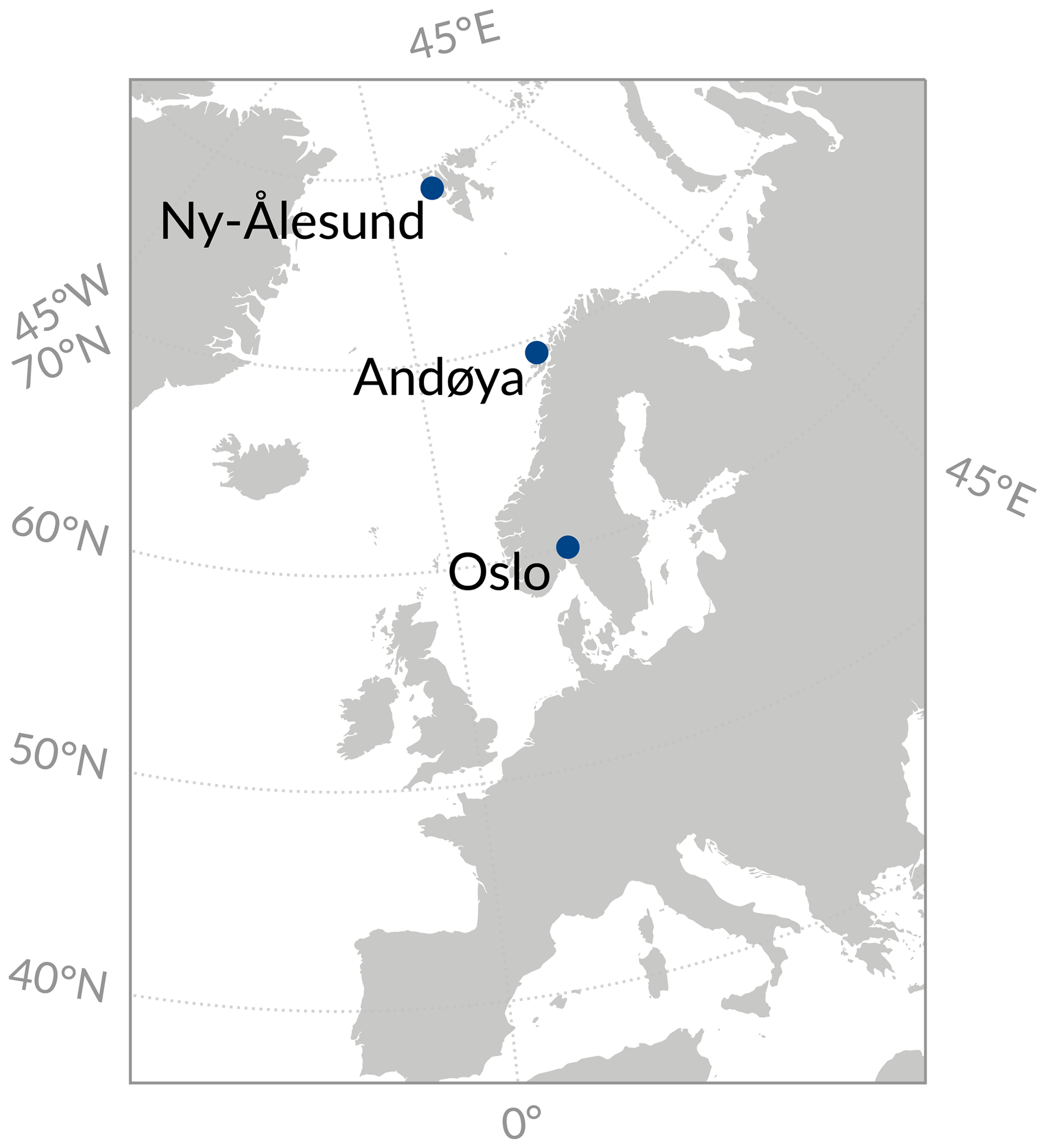
Figure 1 Map of Europe showing the three measurement stations used in this study.

Table 1 Data availability of all instruments used for the combined total ozone time series at the three stations.

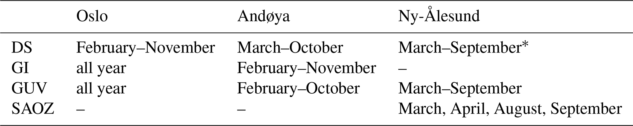
^* After 2013.

2.1 Brewer spectrophotometers

We use ozone data from three Brewer spectrophotometers that measure UV radiation between 305 and 320 nm. The Brewer located at Oslo is a single-monochromator Brewer MKV (serial number B42), whereas a double-monochromator Brewer MKIII (B104) is located at Andøya. Both instruments are operated by NILU and have been calibrated every summer by the International Ozone Service (IOS, Canada) against a reference instrument. No calibrations were performed in 2020 and 2021 due to travel restrictions related to the COVID-19 pandemic. The Brewer at Ny-Ålesund is operated by the National Research Council, Institute of Polar Sciences (CNR-ISP), Italy. It was calibrated by IOS in 2015 and 2018. The Brewer calibration dates are given at https://www.io3.ca/Calibrations (last access: 21 March 2023). We investigated all calibration reports and performed some changes in the calibration files. The updates were small (mainly small calibration date corrections) and affected only a few single days. Measurements during the whole calibration period were excluded.

2.1.1 Direct sun method

For the default direct sun (DS) measurements, the Brewer instrument measures direct sunlight in the UV, as described for example in Savastiouk and McElroy (2005). Total ozone is then derived from the intensities by considering ozone absorption coefficients and Rayleigh scattering coefficients (e.g. Fioletov et al., 2011), using the O3Brewer software (version 6.6 available at http://www.o3soft.eu/o3brewer.html, last access: February 2021). All DS measurements are regularly calibrated with daily standard lamp (SL) measurements. For the SL correction, the intensities of an internal halogen lamp (SL) are measured at the same five wavelengths as for the ozone measurements. The SL produces a stable and continuous light spectrum. Any variations visible in the SL measurements would also affect the ozone measurements and are therefore corrected in the routine DS calculation. The precision of DS measurements is 0.15 % (Scarnato et al., 2010), but the accuracy relies on regular calibrations (Svendby et al., 2021).

2.1.2 Global irradiance method

The Brewer DS method is limited to clear-sky conditions and SZAs below 72^∘. Therefore, we use the global irradiance (GI) method to retrieve ozone from Brewer measurements in cloudy conditions and/or for larger SZA at Oslo and Andøya. In contrast to the DS method, the GI method relies on measurements of diffuse and direct irradiance, including multiple scattering due to clouds and surface reflection. A detailed description of the method and comparison and validation of the GI data is given in Appendix A. The same method has recently been used to derive total ozone from ground-based UV (GUV) radiometers by Svendby et al. (2021).

2.2 GUV

The ground-based UV (GUV) filter radiometers in Oslo (type GUV-511), Andøya, and Ny-Ålesund (both type GUV-541) measure direct and diffuse solar irradiance at five channels in the UV range from 305 to 380 nm. The measurements are used to derive the UV index, total ozone, biological doses, and cloud transmittance (Svendby et al., 2021). GUV ozone retrievals depend on accurate calibrations, and Svendby et al. (2021) showed that the standard deviations between Brewer and GUV in Oslo and at Andøya are within 2.5 % for the period 1995 to 2019. Detailed information about the GUV instruments and the measurement technique can be found in Bernhard (2005) and Svendby et al. (2021). Our GUV data corrections for seasonality and clouds are performed as described by Svendby et al. (2021).

2.3 SAOZ

The SAOZ instrument at Ny-Ålesund measures solar radiation in the UV–visible range of the solar spectrum (300–650 nm). Its measurement principle and basic instrument setup is described in Pommereau and Goutail (1988). Total ozone is retrieved from the measured slant columns at sunrise and sunset, when the SZA is between 86 and 91^∘ (Goutail et al., 2005). In order to convert measured slant columns to vertical columns, ozone air mass factor (AMF) lookup tables are used, calculated using the TOMS V8 ozone profiles (Hendrick et al., 2011). SAOZ ozone measurements present a precision of 4.7 % and an accuracy of 5.9 %. No measurements are available in summer when the SZA is high, and we use SAOZ data only in spring and autumn (see Table 1).

2.4 Combined ground-based total ozone data

To obtain ground-based total ozone time series with as few missing measurement days as possible, we combine total ozone measurements from the four different measurement techniques to a combined time series (GBcomb). Brewer DS and SAOZ have been used in multiple studies (e.g. Hendrick et al., 2011; Goutail et al., 2005; Scarnato et al., 2010) and are therefore used as a baseline in GBcomb. Measurement gaps are then filled with GI and GUV data. GUV data have been validated against Brewer DS and SAOZ data by Svendby et al. (2021), who found no significant biases between the datasets. GI data are evaluated in Appendix A. The Brewer DS measurements build the baseline in Oslo (53 % of the measurement days) and Andøya (44 %). Missing measurement days are first filled with GI data (around 40 % at both stations), then with GUV (5 % in Oslo and 15 % in Andøya) (Fig. 2a, b). In Ny-Ålesund (Fig. 2c), we use SAOZ data as the baseline (around 35 % of the measurements), and days without SAOZ measurements (mainly during summer) are filled with Brewer data (20 % starting in July 2013) and with GUV data (45 % after 2013). In Oslo we have data throughout the year, whereas we have measurements from February or March to October in Andøya. The combined time series at Ny-Ålesund is available from February or March to September or October, depending on the year. For each instrument, we compute daily means of total ozone measurements by considering measurements ±2 h around local noon. Only for SAOZ, daily means of sunset and sunrise measurements are used. Local noon is approximated by the longitude of the station and is 11:15 UTC at Kjeller, 10:55 UTC at Andøya, and 11:12 UTC at Ny-Ålesund. Outliers are excluded when the daily standard deviation exceeds 10 times the mean standard deviation or if the daily mean exceeds 4 times the score z, where $z=({\mathrm{O}}_{\mathrm{3}}-{\stackrel{\mathrm{‾}}{\mathrm{O}}}_{\mathrm{3}}){\text{SD}}^{-\mathrm{1}}$, with the overall mean ozone ${\stackrel{\mathrm{‾}}{\mathrm{O}}}_{\mathrm{3}}$ and the overall standard deviation (SD).

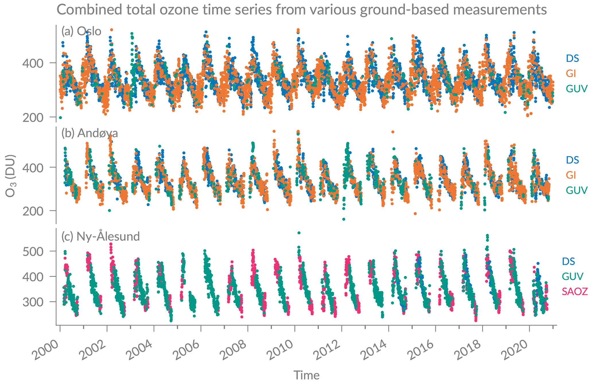
Figure 2 Daily means of total ozone from four different measurement techniques: Brewer direct sun (DS), Brewer global irradiance (GI), ground-based UV (GUV), and SAOZ, measured at (a) Oslo, (b) Andøya, and (c) Ny-Ålesund. DS data are the main dataset in Oslo (a) and Andøya (b), days without DS measurements are filled with GI data, remaining missing data are then filled with GUV measurements. In Ny-Ålesund (c), SAOZ is the main dataset, and DS and GUV are used to fill days with missing SAOZ data.

2.5 Satellites

We use daily means of satellite overpass data from the Ozone Monitoring Instrument (OMI) on the Aura satellite (OMDOAO3 product) launched in 2004 and from two Global Ozone Monitoring Experiment-2 (GOME-2) instruments on the satellites Metop-A (GOME-2A, launched in 2006) and Metop-B (GOME-2B, launched in 2012). In addition we use daily overpass data from the Solar Backscatter Ultraviolet (SBUV) Merged Ozone Dataset (MOD) (SBUV MOD version 2 release 1), which combines total ozone measurements from several SBUV instruments (Frith et al., 2014) processed with a single retrieval algorithm (version 8.7).

2.6 ERA5

We use 2-hourly data on single levels of ERA5, the atmospheric reanalysis from the European Centre for Medium Range Weather Forecasts (ECMWF) (Hersbach et al., 2018, https://doi.org/10.24381/cds.adbb2d47). Various total ozone satellite products are assimilated in ERA5, as described by Hersbach et al. (2020). We use ERA5 data at 10:00 and 12:00 UTC for the grid point closest to each station.

3 Time series comparison

The comparison between the combined ground-based time series (GBcomb), ERA5 reanalysis data, and satellite overpasses is shown in Fig. 3. The GBcomb monthly means are shown in the first row of Fig. 3, complemented by ERA5 data to fill the seasonal measurement gaps (Fig. 3a–c). The seasonal cycle and the interannual variability is clearly visible, as well as the measurement season of the ground-based observations with missing GBcomb data in winter months at Andøya and Ny-Ålesund. The standard deviation of GBcomb data increases with latitude of the station. The second row in Fig. 3 shows the deviation from the climatology (2000–2020), the so-called anomalies. These deseasonalized monthly means show that total ozone varies naturally within around 10 % at Oslo (Fig. 3d) and 20 % at Andøya (Fig. 3e) and Ny-Ålesund (Fig. 3f). The datasets generally agree on the natural variability and the anomalies, with larger anomalies in some years. For example, the ozone-poor year 2020 in the Arctic is clearly visible at Ny-Ålesund (Fig. 3f). Also, the strong negative anomaly in 2011 can be seen in all datasets at all stations. However, we observe that ERA5 reports more total ozone than the other datasets at all stations starting in 2014, which coincides with a change in assimilated satellite data in ERA5, as indicated by Hersbach et al. (2020) (new assimilation of METOP-B GOME-2 and change in assimilated SBUV-2 data). Furthermore, ERA5 and SBUV seem to drift from 2000 to 2005 compared to the ground-based data at all stations. Afterwards, this drift is not visible any more, suggesting that the drift may be corrected with the beginning assimilation of Aura observations in ERA5 (Hersbach et al., 2020).

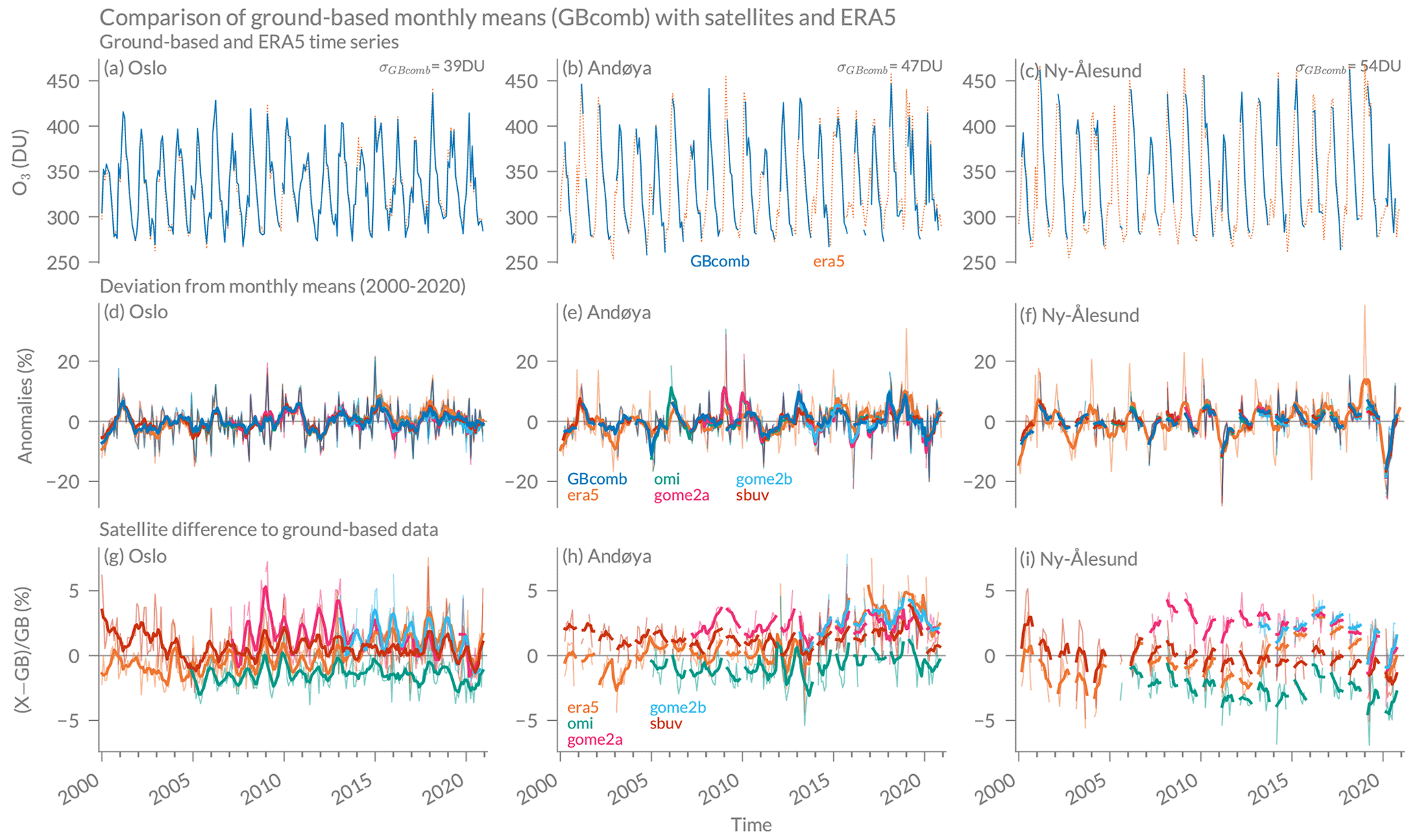
Figure 3 Comparison of the combined ground-based data (GBcomb) with satellite overpasses and ERA5 data at the three stations Oslo, Andøya, and Ny-Ålesund. The first row (a–c) shows monthly means of the ground-based data together with ERA5 monthly means. The standard deviation of GBcomb data (σ_GBcomb) is also given. The second row (d–f) shows relative anomalies for each dataset, which are defined as the deviation of each month from the monthly mean climatology (2000–2020) of the respective dataset. The third row (g–i) shows monthly differences between GBcomb and coincident daily means of the other datasets. The thick lines in panels (d)–(i) show data smoothed with a moving window of 6 months (with a minimum window size of 3 months).

Finally, we compare differences between GBcomb, satellites, and ERA5. For this, we compare daily ground-based measurements with coincident satellite overpasses and ERA5 data and show the monthly means of these differences for each station (Fig. 3g–i). On average, we observe absolute differences of 1 % to 3 % at all stations. This agrees with satellite uncertainties of around 2 % as reported by Bodeker and Kremser (2021). We observe larger deviations for single months, but differences are never larger than 9 %. In Andøya we observe a drift compared to some satellites from 2014 to 2016, which may be related to the issues with the Brewer standard lamp during this period (Sect. A4). However, we found no drift when comparing Brewer with GUV data, which makes the attribution of the origin of the drift difficult. Furthermore, we observe a similar drift when comparing ERA5 with GUV data, suggesting that ERA5 is drifting in this period of new assimilated satellite products (as mentioned above). The drift at Andøya occurs mainly compared to GOME2 and ERA5 and is less visible compared to OMI and SBUV. In Ny-Ålesund, we observe a drift in opposite direction starting in 2016. Further analyses would be required to investigate these differences. Interestingly, most satellites overestimate ozone at Ny-Ålesund in 2016 and underestimate ozone in 2020 compared to the ground-based data; both were years with extreme cold stratospheric conditions. However, GBcomb might slightly overestimate ozone in 2020 due to high Brewer DS values after 2019. The Brewer instrument at Ny-Ålesund was last calibrated by IOS in 2018 and a new calibration and inspection of the instrument will hopefully reveal potential problems.

4 Multiple linear regression

We use a multiple linear regression model that was developed within the activity Long-term Ozone Trends and Uncertainties in the Stratosphere (LOTUS). The so-called LOTUS regression has been tested with several ozone datasets and is described in detail in SPARC/IO3C/GAW (2019). We use the model version 0.8.0 (USask ARG and LOTUS Group, 2017) and extended it by adding additional predictors (see Sect. 4.1). The following regression function is used:

$$\begin{array}{}\text{(1)}& \begin{array}{rl}\widehat{y}\left(t\right)& =a+b\cdot t\\ & +\sum _{n=\mathrm{1}}^{\mathrm{4}}\left(c_n\cdot \sin \left({\displaystyle \frac{\mathrm{2}\mathit{\pi }}{l_n}}\cdot t\right)+d_n\cdot \cos \left({\displaystyle \frac{\mathrm{2}\mathit{\pi }}{l_n}}\cdot t\right)\right)\\ & +\sum _{n=\mathrm{1}}^m\left({\mathit{\beta }}_n{X}_n\right),\end{array}\end{array}$$

with the estimated ozone time series $\widehat{y}\left(t\right)$, the time vector of monthly means t, a constant intercept a, and a linear term b. The seasonal cycle is considered by adding annual oscillations and some overtones (l_n= 12, 6, 4, and 3 months), with fitted coefficients c_n and d_n. In addition, we include m explanatory variables X_n and their fitted coefficients β_n to explain natural variability of ozone. At Ny-Ålesund, only two seasonal components are used (l_n= 12, 6 months) due to the incomplete seasonal cycle because of missing measurements in winter. The regression coefficients are determined by minimizing a cost function, whereas uncertainties of the time series are considered in a full error covariance matrix. The model is iteratively corrected for autocorrelation according to the method by Cochrane and Orcutt (1949) (Damadeo et al., 2014; Appendix B; SPARC/IO3C/GAW, 2019).

The regression is applied to monthly means from the combined daily ozone data (GBcomb). We exclude months with fewer than 25 measurement days to avoid values that are not representative of the whole month. This implies that at Andøya monthly means are excluded for February in several years and from November to January in all years and at Ny-Ålesund from October to February. Monthly ozone uncertainties are considered in the error covariance matrix, using the standard error (SE) of each monthly mean ($\text{SE}={\mathit{\sigma }}_m{n}^{-\frac{\mathrm{1}}{\mathrm{2}}}$, with σ_m the standard deviation of the daily measurements for a particular month and n the number of measurement days for that month). We start our trend analyses in the year 2000, when a general turnaround in ODSs is assumed in polar regions (SPARC/IO3C/GAW, 2019; Weber et al., 2018; Newman et al., 2007; WMO, 2018).

4.1 Regression predictors

The aim of the regression is to assign as much ozone variability as possible to known natural variability by including various predictors. By including the predictors in the regression without detrending them, any trend that is due to long-term changes in one of the predictors is removed from the ozone time series. The remaining, unexplained trend can then be attributed to changes in ODSs (Weber et al., 2022). The LOTUS regression was initially designed to derive stratospheric trend profiles for a broad set of global satellite data (SPARC/IO3C/GAW, 2019). Predictors were selected to obtain a regression that performs best in this setting. The default predictors in the LOTUS regression are the El Niño–Southern Oscillation (ENSO) (e.g. Oman et al., 2013), the Quasi-Biennial Oscillation (QBO) (e.g. Baldwin et al., 2001), solar flux at 10.7 cm wavelength (e.g. Lee, 2003), and aerosol optical depth (AOD) (e.g. Solomon et al., 1998). However, additional predictors may be required when using the regression for local stations, as suggested by Van Malderen et al. (2021) and SPARC/IO3C/GAW (2019). A few recent studies used the LOTUS regression to derive local trend profiles at specific stations (Godin-Beekmann et al., 2022; Bernet et al., 2021; Van Malderen et al., 2021), but they did not investigate the use of additional local predictors. Furthermore, all studies using the LOTUS regression concentrate on latitudes between 60^∘ S and 60^∘ N and on stratospheric ozone profiles. For total ozone trends at higher latitudes, as investigated in our study, other dynamical and chemical predictors can influence ozone variability. A detailed overview about potential predictors that influence total ozone is given for example by Mäder et al. (2007). Various studies investigated how such predictors can be used in multiple linear regressions to derive trends at high latitudes (e.g. Knibbe et al., 2014; Kuttippurath et al., 2015; De Laat et al., 2015; Weber et al., 2022; Pazmiño et al., 2018). We investigate the use of the most relevant predictors in addition to the LOTUS default predictors. For some of them we use local data at the specific stations, and those with a strong seasonal cycle are deseasonalized, as indicated in Table 2. Our study concentrates on stratospheric ozone. The contribution of tropospheric ozone to total ozone is assumed to be small in the study time period and locations (see Sharma et al., 2013; Gaudel et al., 2018), and tropospheric ozone variability is therefore neglected in our trend analysis.

Hersbach et al. (2019,  https://doi.org/10.24381/cds.6860a573 )(Kalnay et al., 1996)(Kalnay et al., 1996)

Table 2 Predictors investigated for use in the multiple linear regression. Predictors that have been used in the final regression are marked in bold.

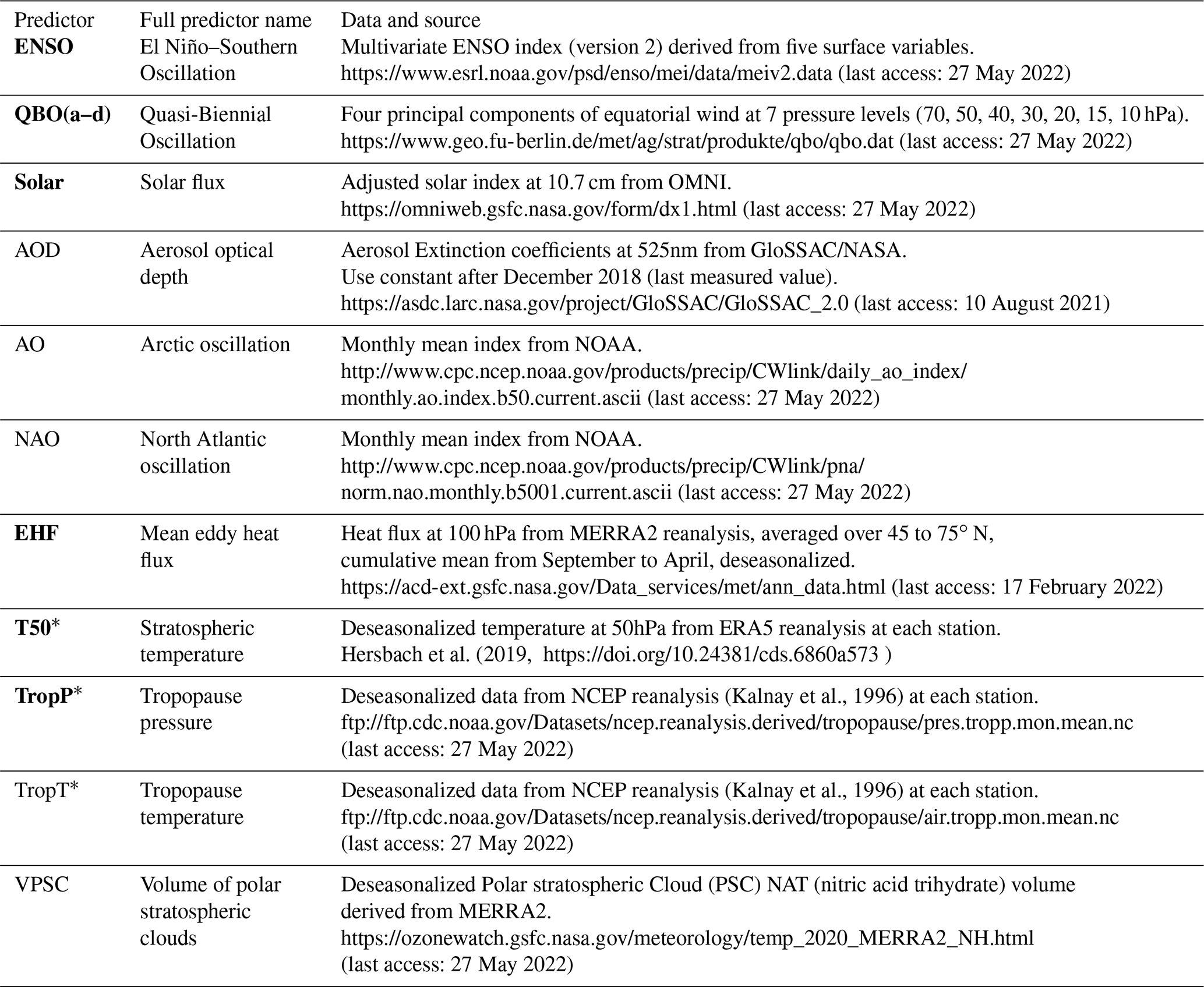
^* Local station-specific data were used for those predictors.

For total ozone, tropopause properties are especially important, as the position of the tropopause has a strong influence on the column amount of ozone (e.g. Wohltmann et al., 2005; Varotsos et al., 2004). An increase in tropospheric height has been recently reported (Thompson et al., 2021; Meng et al., 2021), which may influence ozone trends and should thus be considered in the regression. We therefore investigate the use of station-specific tropopause pressure (TropP) and tropopause temperature (TropT) as predictors. Further, chemical ozone destruction at high latitudes is strongly linked to stratospheric temperature and the occurrence of polar stratospheric clouds (PSCs). We thus inspect the use of a stratospheric temperature predictor at 50 hPa (T50) and an estimator of the PSC volume (VPSC). We also examine the use of some northern teleconnection patterns, namely the Arctic oscillation (AO) and the North Atlantic oscillation (NAO). Such dynamical patterns can have an important effect on total ozone (e.g. Orsolini and Doblas-Reyes, 2003; Appenzeller et al., 2000; Brönnimann et al., 2000). The Brewer–Dobson circulation (BDC) plays an important role in explaining natural ozone variability, especially at high latitudes (e.g. Plumb, 2002). Its strength can be characterized by the upward propagation of planetary waves, represented by the meridional eddy heat flux (EHF) (e.g. Gabriel and Schmitz, 2003). We therefore include the mean EHF at 100 hPa pressure level averaged over 45 to 75^∘ N as a measure of the strength of the BDC. The BDC transports ozone-rich air from the tropics towards the winter pole, and the EHF is strongest in winter. However, the transport-related variability affects not only ozone in winter and spring, but it can also influence the amount of ozone until the following autumn (Fioletov and Shepherd, 2003). We therefore compute a cumulative mean from September to April, as suggested by Weber et al. (2018). Starting in September, each monthly EHF value is computed by averaging from September until the current month. The cumulated cold season mean (September to April) is then also used in the warm season, from May to August.

Finally, we made some adjustments to the default use of QBO terms in the LOTUS regression. The QBO predictor is based on equatorial wind measurements at seven pressure levels. These equatorial oscillations affect ozone beyond the tropics up to polar regions (Wang et al., 2022). However, amplitude, phase, and frequency of the QBO signal may change at higher latitudes (Damadeo et al., 2014). The phase changes and amplitude changes can be considered by using principal components of the seven pressure levels rather than using the direct QBO time series (Damadeo et al., 2014; SPARC/IO3C/GAW, 2019). We use the four leading principal components (QBOa–d) as suggested by Damadeo et al. (2014). Only two components were used in the LOTUS regression so far, but Anstey et al. (2021) showed that additional components are necessary to capture the recent QBO disruption in Northern Hemisphere winter 2019/2020. Furthermore, we added two seasonal components to the QBO predictors. This is important because a seasonal dependence of QBO is observed at higher latitudes (Tung and Yang, 1994; Damadeo et al., 2014), which is generally not captured by regression models (Ball et al., 2019). Also, Godin-Beekmann et al. (2022) showed that the regression fit improves when seasonal components of predictors are included in the LOTUS regression.

4.2 Final choice of predictors

A multiple linear regression is based on the assumption that the predictors are independent. For our final selection of predictors, we therefore investigate the predictors' correlations. The Pearson correlation coefficient r for all the predictors that we investigated at Oslo are shown in Fig. 4. The significance of each coefficient has been tested with a p value of 0.05, using a multiple test to reduce the possibility that a correlation is significant by chance (adjusted p value). Some predictors can immediately be excluded because of their high correlation to another predictor. For example, tropopause pressure (TropP) and tropopause temperature (TropT) should not be used both because they are significantly correlated (r=0.91). We decide to use TropP and not TropT because the tropopause altitude has a large influence on total ozone (e.g. Steinbrecht et al., 1998; Varotsos et al., 2004). Furthermore, the circulation patterns NAO and AO are significantly correlated (r=0.62) and should not be used both in the regression. TropP and T50 are also significantly correlated (r=0.51), but their simultaneous use is further discussed below. Finally, there is a significant correlation between AOD and the solar flux ($r=-\mathrm{0.51}$). This might be a spurious correlation in the selected time period, where AOD was generally low because no major volcanic eruption occurred. Indeed, no correlation between solar flux and AOD is observed for a longer time period from 1979 to 2020 (not shown). The ozone effect from AOD is mainly relevant for important volcanic eruptions (e.g. Solomon et al., 1998), and we therefore decide not to use AOD in our regression.

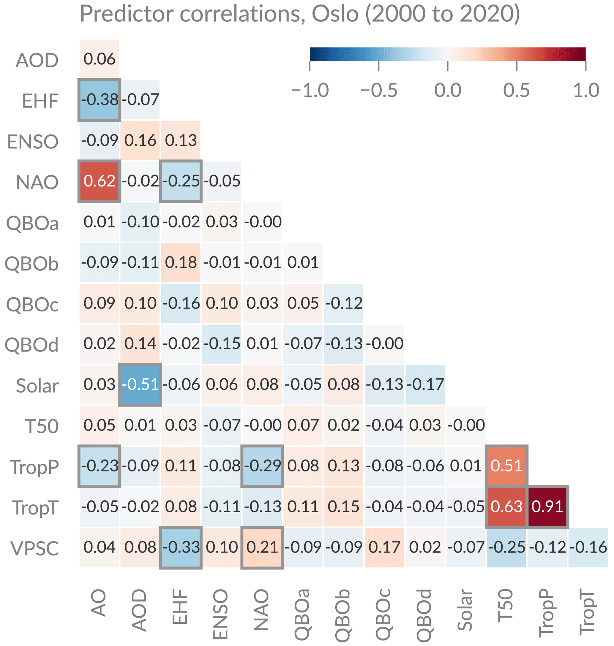
Figure 4 Pearson correlation coefficients of various predictors that are commonly used to account for natural ozone variability. The predictors that are location-specific are shown for Oslo (TropP, TropT, and T50); the other predictors are station-independent. Significant correlations are marked by a grey border. The significance has been tested with a p value of 0.05 using a multiple test to reduce the possibility that a correlation is significant by chance (adjusted p value).

Besides the independence and the physical meaningfulness of the predictors, it is important to study the improvement of the regression fit when a specific predictor is included. Based on these aspects, we decided on a final set of predictors used in the regression fit. First, we decided to use T50, even though it is correlated to TropP, because including T50 substantially improves the adjusted coefficient of determination ($R_{\mathrm{adj}}^{\mathrm{2}}$) of the annual model fit (e.g. from 0.91 to 0.96 at Oslo) and for most months. To be sure that the correlation between both does not affect the interpretation of our results, we also inspected the fit for a possible multicollinearity by investigating the variance inflation factor (VIF). We used a VIF threshold of 5, which means that no collinearity problem is assumed when testing the regression with each predictor as dependent variable as long as VIF <5 (e.g. Schuenemeyer and Drew, 2010). We observed multicollinearity only for monthly trends at Oslo in March (VIF_TropP=5.2) and September (VIF_T50=5.5) and at Ny-Ålesund in September (VIF_TropP=5.0), but not for annual trends.

Second, we decided not to include the dynamical predictors NAO and AO, because they are weakly but significantly correlated with TropP and EHF (Fig. 4). These large-scale predictors should be well represented in the local predictors (TropP), as also suggested by Mäder et al. (2007). Also, there is no important improvement in the model performance when NAO and AO predictors are included. Finally, we do not include VPSC because of the weak but significant correlation to EHF (Fig. 4) and no general improvement in $R_{\mathrm{adj}}^{\mathrm{2}}$, even though we observe that the fit at Ny-Ålesund is improved (smaller residuals) in some extreme years when VPSC is included (not shown). The temperature-dependent chemical activity is already covered by using T50, which in addition represents circulation changes in the stratosphere. The chosen predictors that are finally used in the regression are marked in bold in Table 2.

Figure 5 shows the contribution of the selected predictors to the regression fit at Oslo using the full time series, further referred to as annual trend fit. The model is well representing the data with a $R_{\mathrm{adj}}^{\mathrm{2}}$ of 0.96, which indicates that the regression fit can explain 96 % of the ozone variation at Oslo. The residuals generally lie within 5 % and a spectral analysis of the residuals (not shown) suggests that the dominant patterns that influence ozone variation are captured by the regression. The lower panels in Fig. 5 show that most of the ozone variation can be explained by T50 and TropP (predictors with largest contribution), followed by two of the QBO terms (QBOb and QBOc). The solar flux, ENSO, and EHF have only small contributions to ozone variability at Oslo. However, all predictors have a significant contribution to the regression fit except the EHF and three of the QBO components (see annual trend in Fig. 6). At Andøya and Ny-Ålesund, the EHF contribution to the annual fit is significant, but some of the default predictor coefficients (Solar, ENSO, and QBO) become insignificant (see Figs. B1 and B2). This confirms results by Bahramvash Shams et al. (2019) based on ozonesonde measurements in the Arctic and by Vigouroux et al. (2015) based on FTIR measurements.

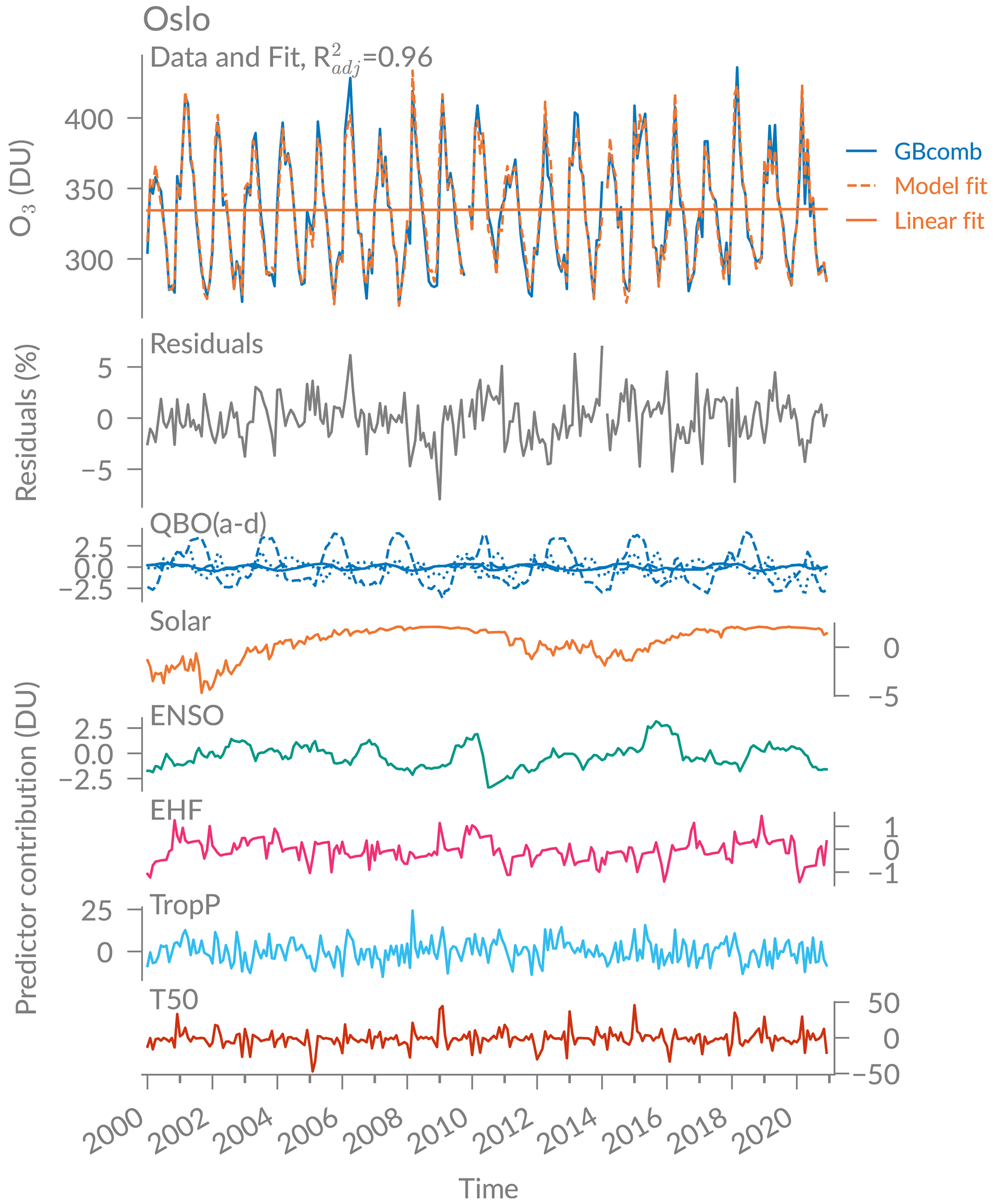
Figure 5 Regression fit, residuals, and predictor contribution (β_n⋅X_n, with coefficient β_n and predictor X_n) at Oslo.

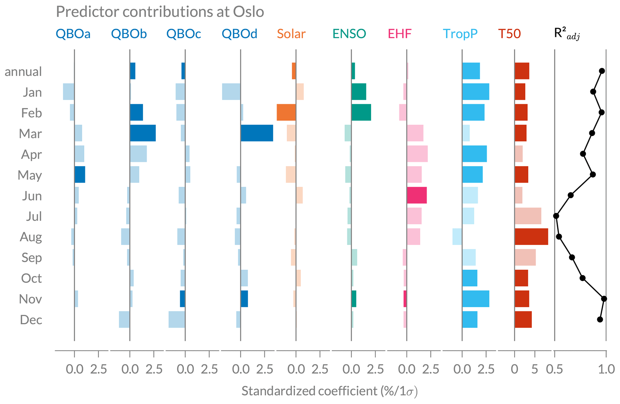
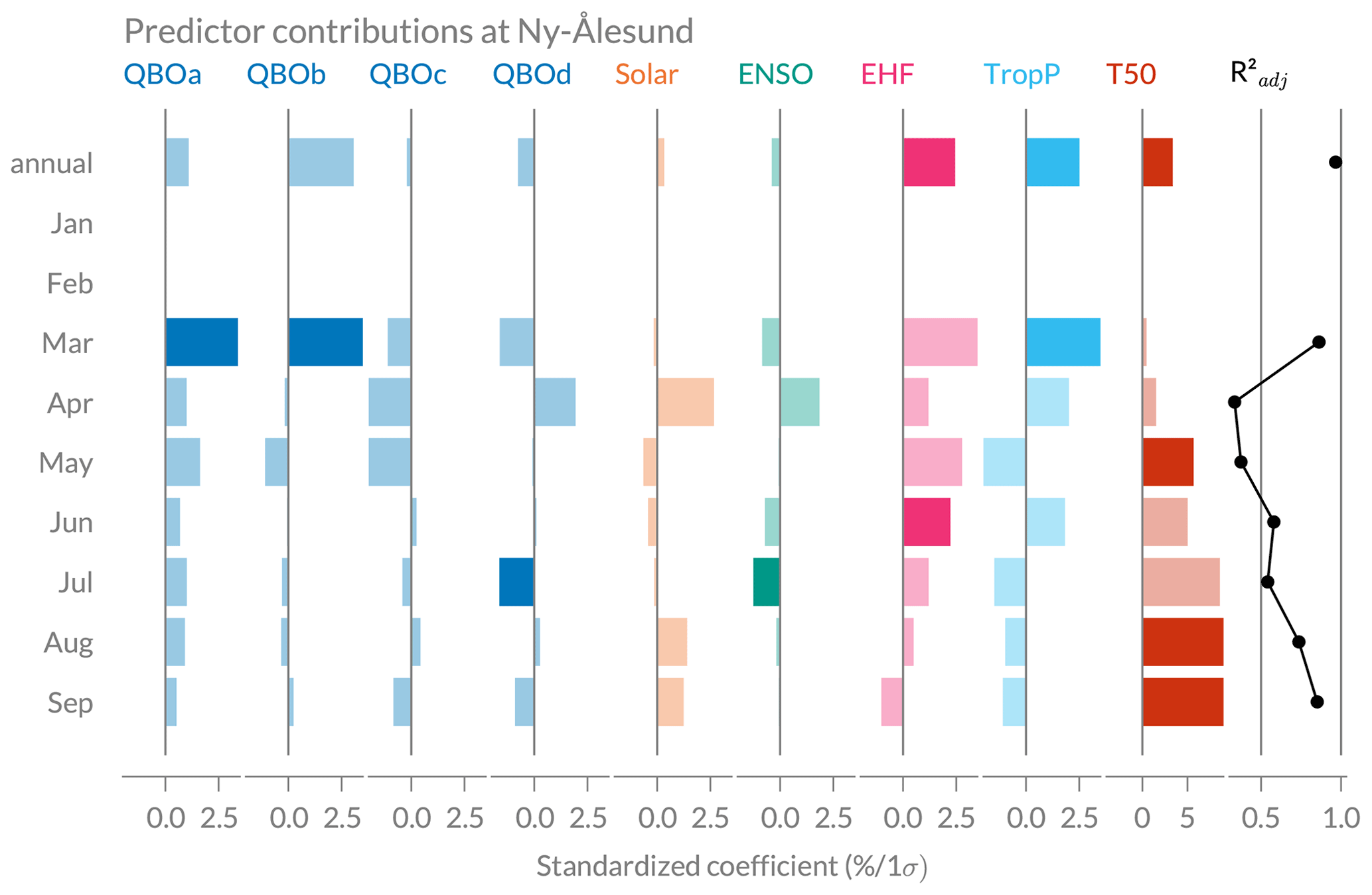
Figure 6 Predictor contribution to the regression fit at Oslo for the annual regression fit and individual monthly fits. The standardized coefficients describe the percentage change in ozone for a 1σ change in the predictor. Pale colour bars indicate that the predictor's contribution to ozone is not significant (p value of the coefficient <0.05). The last panel on the right shows the adjusted coefficient of determination ($R_{\mathrm{adj}}^{\mathrm{2}}$) for the annual and all monthly fits. Note that the range of the x axis is different for T50 than for the other predictors.

The predictor coefficients, their significance, and the model’s performance for individual monthly fits at Oslo are shown in Fig. 6. The coefficients have been standardized to make a direct comparison possible. The standardized coefficients β_std describe the percentage change in ozone for a 1σ change in the predictor, according to Brunner et al. (2006):

$$\begin{array}{}\text{(2)}& {\mathit{\beta }}_{\mathrm{std}}=\mathit{\beta }{\displaystyle \frac{{\mathit{\sigma }}_X}{\stackrel{\mathrm{‾}}{y}}}\cdot \mathrm{100},\end{array}$$

with the predictor coefficient β, the standard deviation σ_X of predictor X, and the mean ozone value $\stackrel{\mathrm{‾}}{y}$. Generally, the largest contribution to total ozone is provided by the T50 predictor, followed by TropP (Fig. 6). Whereas most predictors contribute significantly to the annual regression fit and to most monthly fits in winter, the regression coefficients are mostly insignificant in the summer months (pale shading in Fig. 6). This poor explanation of ozone variability in summer by the predictors is reflected in lower values of $R_{\mathrm{adj}}^{\mathrm{2}}$ from June to September ($R_{\mathrm{adj}}^{\mathrm{2}}$ between 0.5 and 0.7), with particular low values in July and August (0.51 and 0.54). In most other months, however, the ozone variation at Oslo is well captured by the model, with $R_{\mathrm{adj}}^{\mathrm{2}}$ ranging from 0.77 (October) to 0.98 (November). Total ozone in summer is generally driven by photochemistry and less by the transport-related predictors, which may explain the poorer model performance in summer. Furthermore, the interannual variability is generally low in summer and may be dominated by natural variability or noise, as suggested by Brunner et al. (2006).

In Ny-Ålesund and Andøya, we observe high $R_{\mathrm{adj}}^{\mathrm{2}}$ in March and September and smaller values in the other months, especially in April (both stations) and May (only at Ny-Ålesund) (see Figs. B1 and B2). However, the $R_{\mathrm{adj}}^{\mathrm{2}}$ at those stations is generally lower than in Oslo, especially at Ny-Ålesund. This can be explained by the high interannual variability at Andøya and Ny-Ålesund (compare Fig. 3) that makes it more difficult to explain the ozone variability with the predictors used.

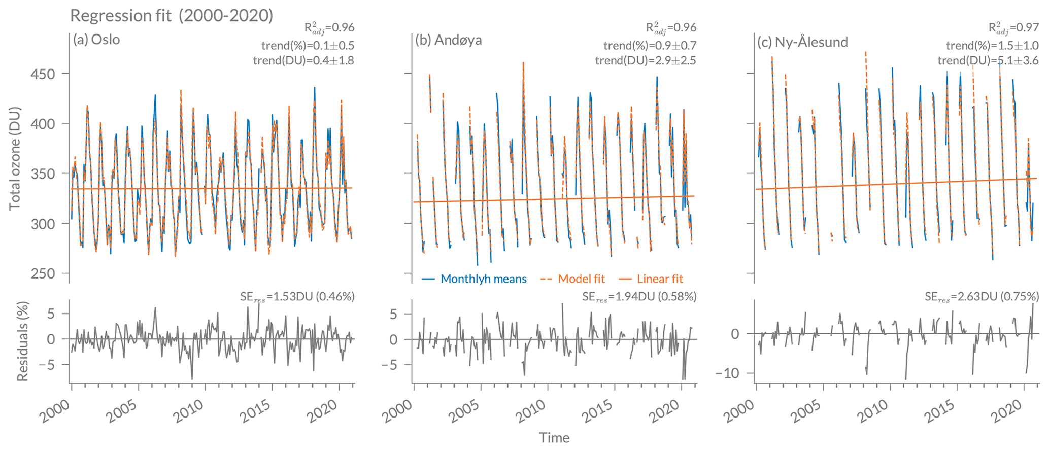
Figure 7 Regression fit of total ozone for (a) Oslo, (b) Andøya, and (c) Ny-Ålesund. The resulting linear trend is given in percent per decade and DU per decade with 2-standard-deviation (σ) uncertainties. The lower panels show the residuals of the regression fit in percent $\left(\right(\text{Data}-\text{Model})/\text{Data})$ and the standard error of the residuals (SE_res) in DU and percent (compared to the mean ozone value at each station).

5 Trend results

5.1 Annual trends

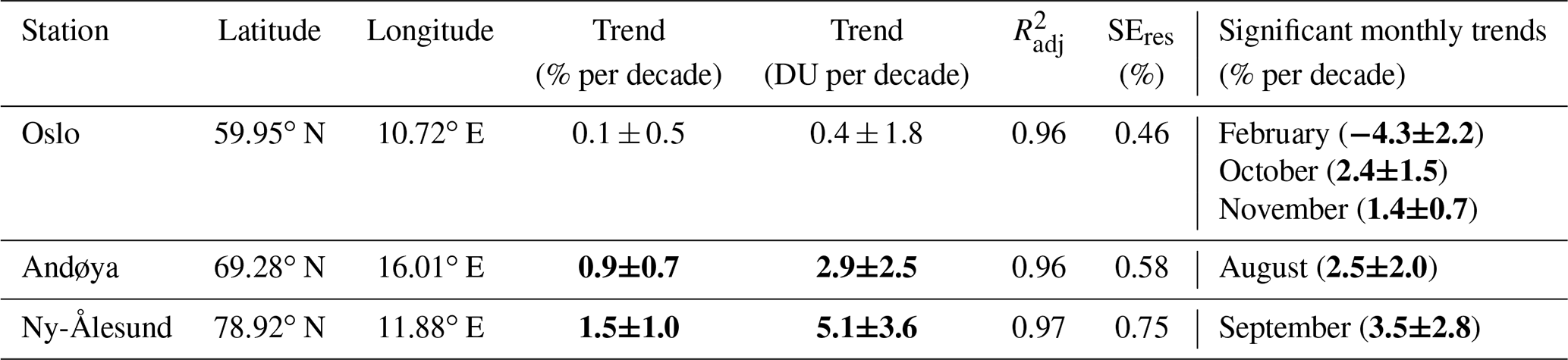
Annual trend fits (using the full time series) and their residuals for the three stations are shown in Fig. 7 and represented in Table 3. At all stations, we observe that the model represents the data well, with $R_{\mathrm{adj}}^{\mathrm{2}}$ values of 0.96 (Oslo and Andøya) and 0.97 (Ny-Ålesund). The residuals lie within 5 %, with some outliers of up to 10 % in Andøya and Ny-Ålesund, where the model captures less well the ozone variability (e.g. in 2008 or 2020). The standard errors of the residuals (SE_res) of 1.53 DU (Oslo) to 2.63 DU (Ny-Ålesund) indicate that the predicted values differ from the true ozone values by less than 1 % on average. We observe significant positive total ozone trends at Andøya and Ny-Ålesund of 0.9±0.7 % per decade and 1.5±1.0 % per decade, respectively, and a trend of almost zero (0.1±0.5 % per decade) at Oslo (see Fig. 7 and Table 3). Trends are expressed as percentage of the mean ozone value at each station, and a trend is declared to be significantly different from zero at a 95 % confidence interval as soon as its absolute value exceeds twice its uncertainty (e.g. Tiao et al., 1990).

Table 3 Trend values for annual regression fits of total ozone (2000 to 2020) with $R_{\mathrm{adj}}^{\mathrm{2}}$ and the standard errors of the residuals (SE_res). Trends that are significantly different from zero at 95 % confidence interval are marked in bold. The second column shows monthly trends that are significantly different from zero.

Positive trends of similar magnitudes have also been found for Scandinavia or the North Atlantic in previous satellite-based studies. For example, Sofieva et al. (2021) found positive trends over Scandinavia of 1 % per decade to 5 % per decade depending on altitude based on merged satellite ozone profile data from 2003 to 2018 (their Fig. 10), and Coldewey-Egbers etal. (2022) reported significantly positive total ozone trends of 1.2 % per decade in the North Atlantic sector based on merged total ozone data from 1997 to 2020 (their Table 3 and Fig. 3). Furthermore, Svendby et al. (2021) analysed total ozone trends with a simple linear regression from 1999 to 2019, using ground-based GUV measurements at the same three stations as in our study. They found similar trend magnitudes but slightly larger uncertainties (1.5±1.8 % per decade at Oslo, 0.5±2.6 % per decade at Andøya, 1.2±2.4 % per decade at Ny-Ålesund). In contrast to our results at Andøya and Ny-Ålesund, their annual trends were not significant, which suggests that the use of multiple predictors in our study can successfully reduce trend uncertainties at the two northernmost stations.

5.2 Monthly trends

Monthly trends were computed for all stations by applying the regression to the time series of each month, usually including 21 data points for each month (2000 to 2020). We do not include February trends at Andøya because the time series is short (only 15 years) due to sparse February measurements in some years. The monthly trends are illustrated in Fig. 8, and significant trends are given in Table 3.

Figure 8 Monthly ozone trends in percent per decade for the three stations, with 2σ uncertainty shadings. Filled dots represent trends that are significantly different from zero at the 95 % confidence interval. Fits with low $R_{\mathrm{adj}}^{\mathrm{2}}<\mathrm{0.5}$ are marked with crosses.

Trends in late spring and summer months (May to July) are not significantly different from zero at 95 % confidence interval at all stations and almost zero at Oslo. However, in late summer and autumn (August to November), we observe significant positive ozone trends at Oslo (October: 2.4±1.5 % and November: 1.4±0.7 % per decade), Andøya (August: 2.5±2.0 %), and Ny-Ålesund (September: 3.5±2.8 % per decade). Our significant autumn trends confirm results by Svendby et al. (2021), who found significant trends at Oslo of 3.23±2.01 % in fall from 1999 to 2019 using a simple linear regression. In contrast to our results, Morgenstern et al. (2021) found significant negative trends in September and October at 80^∘ N, using satellite zonal means. These contrasting results suggest that it is important to investigate regional trends and not only zonal means.

In winter (December to February), we only derive trends in Oslo due to the missing data (polar night) at the other stations. Winter Oslo trends are positive but insignificant in December and January and significantly negative in February ($-\mathrm{4.3}\pm \mathrm{2.2}$ % per decade). The negative February trend in Oslo persists even if we exclude the extreme year 2020 from the regression. This negative trend may be specific for the selected time period: in the first 5 years (2000–2005) we have rather stable February monthly means; afterwards we observe more interannual variability and several years with specially low ozone, which results in a negative trend. Furthermore, we observe a significant negative contribution of the solar predictor to February ozone at Oslo as visible in Fig. 6. Longer time series and additional stations would need to be investigated to analyse this effect further. Interestingly, the Oslo February fit is remarkably good compared to other months, with a $R_{\mathrm{adj}}^{\mathrm{2}}$ of 0.96 (see Fig. 6), indicating that the predictors used can well capture the high year-to-year variability in February.

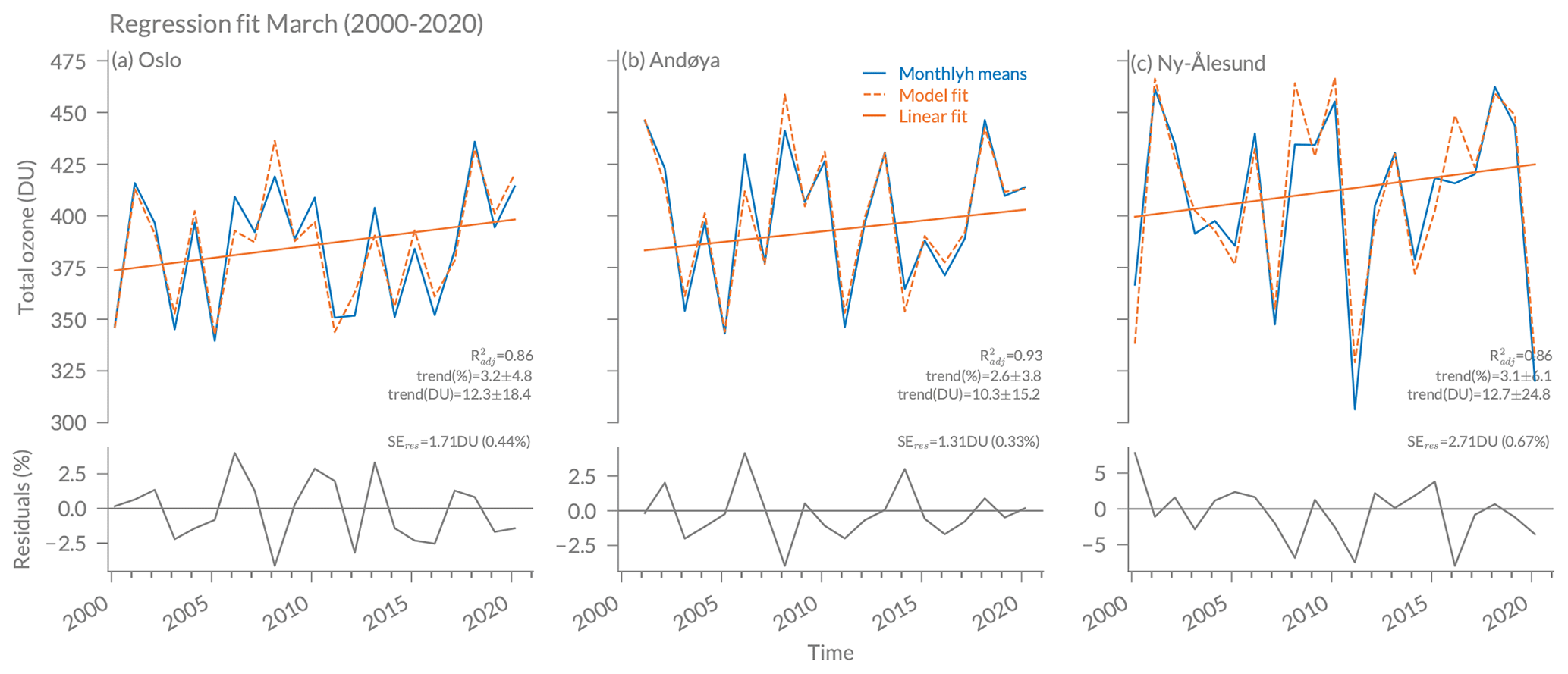
Ozone trends in spring months are of special interest in polar regions, because those regions experienced strongest ozone depletion in the pre-2000 phase (e.g. Solomon, 1999). At the two northernmost stations (Ny-Ålesund and Andøya), our analyses report positive but insignificant ozone trends in March and April. The trend uncertainties are high, related to the large interannual variability. In April, the model fit is not as good as in most other months, with $R_{\mathrm{adj}}^{\mathrm{2}}$ of 0.33 (Ny-Ålesund) and 0.49 (Andøya), indicating that April ozone variability is less well explained by the predictors used in our regression. In March, however, $R_{\mathrm{adj}}^{\mathrm{2}}$ values are at least 0.86 at all three stations. The March time series and the corresponding regression fits are shown in Fig. 9. Even though the March trends are not significantly different from zero (at 95 % confidence) due to large trend uncertainties, it is remarkable that all three station data agree on similar positive ozone trends of around 3 % per decade and that the regression model can reproduce the ozone variability so well. Positive but insignificant March trends in the Arctic (60 to 90^∘ N) have also been reported by Weber et al. (2018) based on zonal satellite and ground-based data; they found trends of 1.2±3.7 % per decade (with 2σ uncertainties) from 2000 to 2016 and slightly larger trends when extending to 2020 (2.0±3.9 %; Weber et al., 2022). Our March trends at the three stations are slightly larger than those zonal mean trends. These results confirm previous studies reporting zonally asymmetric trends with larger trends over the Atlantic and Scandinavian sector compared to other longitudes at northern high latitudes (Zhang et al., 2019; Sofieva et al., 2021; Coldewey-Egbers etal., 2022).

Figure 9 Same as Fig. 7 but for the month of March.

6 Conclusions

This study investigates ground-based total ozone trends at the northern high-latitude stations Oslo, Andøya, and Ny-Ålesund. We presented combined total ozone time series at the three stations with measurements from four measurement techniques (Brewer DS, Brewer GI, SAOZ, and GUV). The combination of various techniques makes it possible to overcome measurement gaps due to instrumental limitations. The combined time series were compared with satellite overpass data and ERA5 reanalysis. All datasets agree on average within 1 % to 3 % with the ground-based time series.

To derive total ozone trends from 2000 to 2020, we used the LOTUS regression model for the first time for ground-based total ozone data at high latitudes. Additional regression predictors have been examined, and a set of predictors have been identified that should be considered when deriving total ozone trends at northern high latitudes. We examined various predictors that are commonly used to account for natural ozone variability by checking their correlations and contributions to the regression fit. We found that tropopause pressure and lower-stratospheric temperature are dominant predictors that contribute significantly to ozone in most months. Our results further show that the trend model with the selected predictors represents well the total ozone variability at the selected stations, with high coefficients of determination ($R_{\mathrm{adj}}^{\mathrm{2}}>\mathrm{0.95}$). We found significant trends of 0.9 % per decade at Andøya and 1.5 % per decade at Ny-Ålesund, but no significant trends at Oslo when looking at the full time series (annual trends). Our monthly regression analyses indicate significant positive trends in autumn at Oslo (October and November) and late summer at the northernmost stations Andøya and Ny-Ålesund (August or September). Finally, we observe positive trends of around 3 % per decade in Arctic spring (March), but the trends are not significantly different from zero. Nevertheless, these springtime trends and the significant autumn trends might be an indication for Arctic ozone recovery due to changes in ODSs.

In conclusion, our study emphasizes the need to concentrate on regional ozone trends rather than zonal means when investigating Arctic ozone recovery. Long-term ground-based measurements of total ozone can contribute to this aim by verifying satellite-derived trends on a regional scale. Our results contribute to a better understanding of regional total ozone trends at northern high latitudes, which is essential to assess how Arctic ozone responds to changes in ODSs and to climate change.

Appendix A: Global irradiance (GI) method

A1 GI retrieval

The most accurate estimates of total ozone amount in the atmosphere with the Brewer spectrophotometer use direct sun (DS) measurements. The DS procedure is based on simultaneous measurements of direct solar radiation I_i at four UV wavelengths ($i=\mathrm{2},\mathrm{3},\mathrm{4},\mathrm{5}$) with different ozone absorption coefficients. The wavelengths used are 310.1, 313.5, 316.8, and 320.1 nm, all with a 0.6 nm bandwidth (full width at half maximum, FWHM) (SCI-TEC Instruments, 1999). Combining the radiation at the four wavelengths we obtain the following:

$$\begin{array}{}\text{(A1)}& N(x,{\mathit{\theta }}_{\mathrm{s}})={\displaystyle \frac{I_{\mathrm{4}}(x,{\mathit{\theta }}_{\mathrm{s}})}{I_{\mathrm{2}}(x,{\mathit{\theta }}_{\mathrm{s}})}}\cdot {\left({\displaystyle \frac{I_{\mathrm{4}}(x,{\mathit{\theta }}_{\mathrm{s}})}{I_{\mathrm{3}}(x,{\mathit{\theta }}_{\mathrm{s}})}}\right)}^{-\mathrm{0.5}}\cdot {\left({\displaystyle \frac{I_{\mathrm{5}}(x,{\mathit{\theta }}_{\mathrm{s}})}{I_{\mathrm{4}}(x,{\mathit{\theta }}_{\mathrm{s}})}}\right)}^{-\mathrm{1.7}},\end{array}$$

where x is the ozone amount and θ_s is the solar zenith angle (SZA). The values −0.5 and −1.7 are weights that minimize effects of SO₂ absorption on N(x,θ_s). Radiances of direct sunlight passing through the atmosphere are attenuated according to Beer's law. As the ozone absorption coefficients and molecular scattering cross-sections for the different wavelengths used are known, the total ozone amount x can be found by taking the logarithm of N and considering the known absorption coefficients, the air mass factor, and the background intensity (see e.g. Savastiouk and McElroy, 2005, WMO, 2008, chap. 16, Fioletov et al., 2011).

When clouds obscure the sun, the radiances I do not obey Beer's law because diffuse (scattered) radiation becomes important. Therefore, the simple logarithm procedure fails. In the GI (global irradiance) method, the radiances I in Eq. (A1) are replaced by irradiances E, i.e. the sum of the direct and diffuse radiation falling on a flat horizontal surface. The global irradiances are measured through the UV dome of the Brewer instead of the flat quartz window used for DS measurements. The modified radiation for GI, N_GI(x,θ_s), is

$$\begin{array}{}\text{(A2)}& \begin{array}{rl}{N}_{\mathrm{GI}}(x,{\mathit{\theta }}_{\mathrm{s}})& ={\displaystyle \frac{E_{\mathrm{4}}(x,{\mathit{\theta }}_{\mathrm{s}})}{E_{\mathrm{2}}(x,{\mathit{\theta }}_{\mathrm{s}})}}\cdot {\left({\displaystyle \frac{E_{\mathrm{4}}(x,{\mathit{\theta }}_{\mathrm{s}})}{E_{\mathrm{3}}(x,{\mathit{\theta }}_{\mathrm{s}})}}\right)}^{-\mathrm{0.5}}\\ & \cdot {\left({\displaystyle \frac{E_{\mathrm{5}}(x,{\mathit{\theta }}_{\mathrm{s}})}{E_{\mathrm{4}}(x,{\mathit{\theta }}_{\mathrm{s}})}}\right)}^{-\mathrm{1.7}}.\end{array}\end{array}$$

The N_GI(x,θ_s) is simulated with a multiple scattering pseudo-spherical radiative transfer model (Stamnes et al., 1988; Dahlback and Stamnes, 1991) for various x and θ_s to obtain a lookup table. Light scattering on air molecules depends strongly on wavelength (Rayleigh scattering). In clouds, the wavelength dependency is considerably smaller due to the much larger sizes of cloud particles compared to air molecules (Mie scattering). Since the N_GI values are based on irradiance ratios, the sensitivity to clouds is expected to be small, at least for thin clouds. Thus the lookup table is calculated for clear sky and a surface albedo of 5 % pertinent for snow- and ice-free surfaces. The sensitivity of ozone profiles to the irradiances (and hence the N_GI values) increases with θ_s. Therefore, a profile climatology for low, middle, or high latitudes (McPeters et al., 1998) can be chosen to compute the N_GI value lookup tables. The ozone amount x is then determined by finding the N_GI value in the lookup table that agrees with the observed N_GI.

A2 GI calibration

The radiation detector in the Brewer is a photomultiplier tube (PMT). The irradiance for a particular wavelength is proportional to its count rate C_i ($i=\mathrm{2},\mathrm{3},\mathrm{4},\mathrm{5}$). The N_GI value can be written as

$$\begin{array}{}\text{(A3)}& \begin{array}{rl}{N}_{\mathrm{GI}}(x,{\mathit{\theta }}_{\mathrm{s}})& =r\cdot {\displaystyle \frac{C_{\mathrm{4}}(x,{\mathit{\theta }}_{\mathrm{s}})}{C_{\mathrm{2}}(x,{\mathit{\theta }}_{\mathrm{s}})}}\cdot {\left({\displaystyle \frac{C_{\mathrm{4}}(x,{\mathit{\theta }}_{\mathrm{s}})}{C_{\mathrm{3}}(x,{\mathit{\theta }}_{\mathrm{s}})}}\right)}^{-\mathrm{0.5}}\\ & \cdot {\left({\displaystyle \frac{C_{\mathrm{5}}(x,{\mathit{\theta }}_{\mathrm{s}})}{C_{\mathrm{4}}(x,{\mathit{\theta }}_{\mathrm{s}})}}\right)}^{-\mathrm{1.7}},\end{array}\end{array}$$

where r is a calibration factor that is determined by utilizing a reliable ozone DS measurement with the Brewer. By choosing a day with clear sky, preferably around noon, the r value is determined such that Eq. (A3) agrees with the N_GI value in the lookup table for the observed DS ozone value and SZA θ_s. We performed a GI calibration as soon as we observed severe changes in the Brewer standard lamp (SL). In Andøya, we calibrated GI in June 2001, August 2014, August 2016, August 2018, and August 2019, for Oslo we used new calibration files in August 2005 and twice in summer 2019 (see Fig. A2).

The Oslo Brewer is equipped with a single monochromator. It is well known that stray light in the single Brewer optics causes errors in measured ozone at large θ_s and particularly for large ozone amounts. Therefore, for low sun (${\mathit{\theta }}_{\mathrm{s}}>\mathrm{72}{}^{\circ }$) we replace the four-wavelength ratios in Eqs. (A2) and (A3) by a single ratio of 316.8 to 313.5 nm. The motivation for this is that we avoid 310.1 nm radiation, which is the wavelength that is mostly affected by stray light in Eq. (A2).

In order to filter out cases where thick clouds are difficult to correct, we define a cloud transmission factor CLT:

$$\begin{array}{}\text{(A4)}& \text{CLT}=\text{cr}\cdot {\displaystyle \frac{C_{\mathrm{5},\mathrm{meas}}(x,{\mathit{\theta }}_{\mathrm{s}})}{E_{\mathrm{5},\mathrm{clearsky}}(x,{\mathit{\theta }}_{\mathrm{s}})}}.\end{array}$$

C_5,meas is the measured irradiance (count rate), and E_5,clearsky is the clear-sky irradiance calculated with the radiative transfer model for a snow- and ice-free surface. The factor cr is a calibration factor that is determined by using measurements on a day with cloud-free and snow-free conditions with CLT=1 (100 %).

A3 GI processing

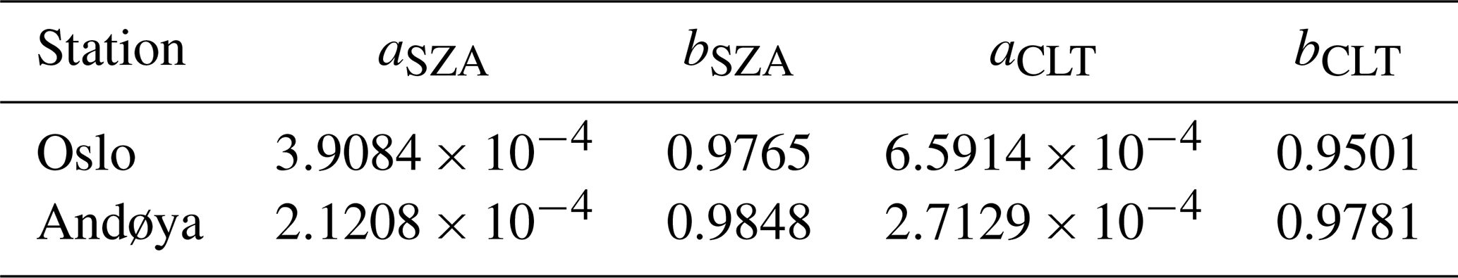
The GI method described above will normally work well without further corrections. However, to optimize the measurements, we have taken instrumental drift (SL changes) into account, as described in Sect. 2.1.1 for DS measurements. Further, we performed minor cloud and SZA corrections, based on the comparison to DS measurements. Similar corrections have been used by Svendby et al. (2021) on measurements from ground-based UV (GUV) radiometers. The SZA correction is mainly relevant for the winter season when the combination of a changed atmospheric profile and low sun can introduce errors to the ozone value retrieved from the lookup table. To obtain corrected GI values (GI_corr), we derive a correction function f(i) from the linear relationship between the DS $/$ GI ratio and the solar angle (i=SZA) as well as DS $/$ GI and the cloud transmittance (i=CLT):

$$\begin{array}{}\text{(A5)}& {\text{GI}}_{\mathrm{corr}}\left(t\right)=\text{GI}\left(t\right)\cdot f\left(i\right),\end{array}$$

with

$$\begin{array}{}\text{(A6)}& f\left(i\right)={\displaystyle \frac{\text{DS}\left(i\right)}{\text{GI}\left(i\right)}}=a_i\cdot i+b_i.\end{array}$$

The correction coefficients are derived by comparing GI to DS measurements from 1995 to 2020 in Oslo and from 2000 to 2020 in Andøya, as shown in Fig. A1. The derived coefficients are given in Table A1. The CLT correction is only applied for cloudy situations (CLT<90 %). Finally, we excluded GI data for situations with low cloud transmittance (CLT<20 %) and situations with ${\mathit{\theta }}_{\mathrm{s}}>\mathrm{84}{}^{\circ }$.

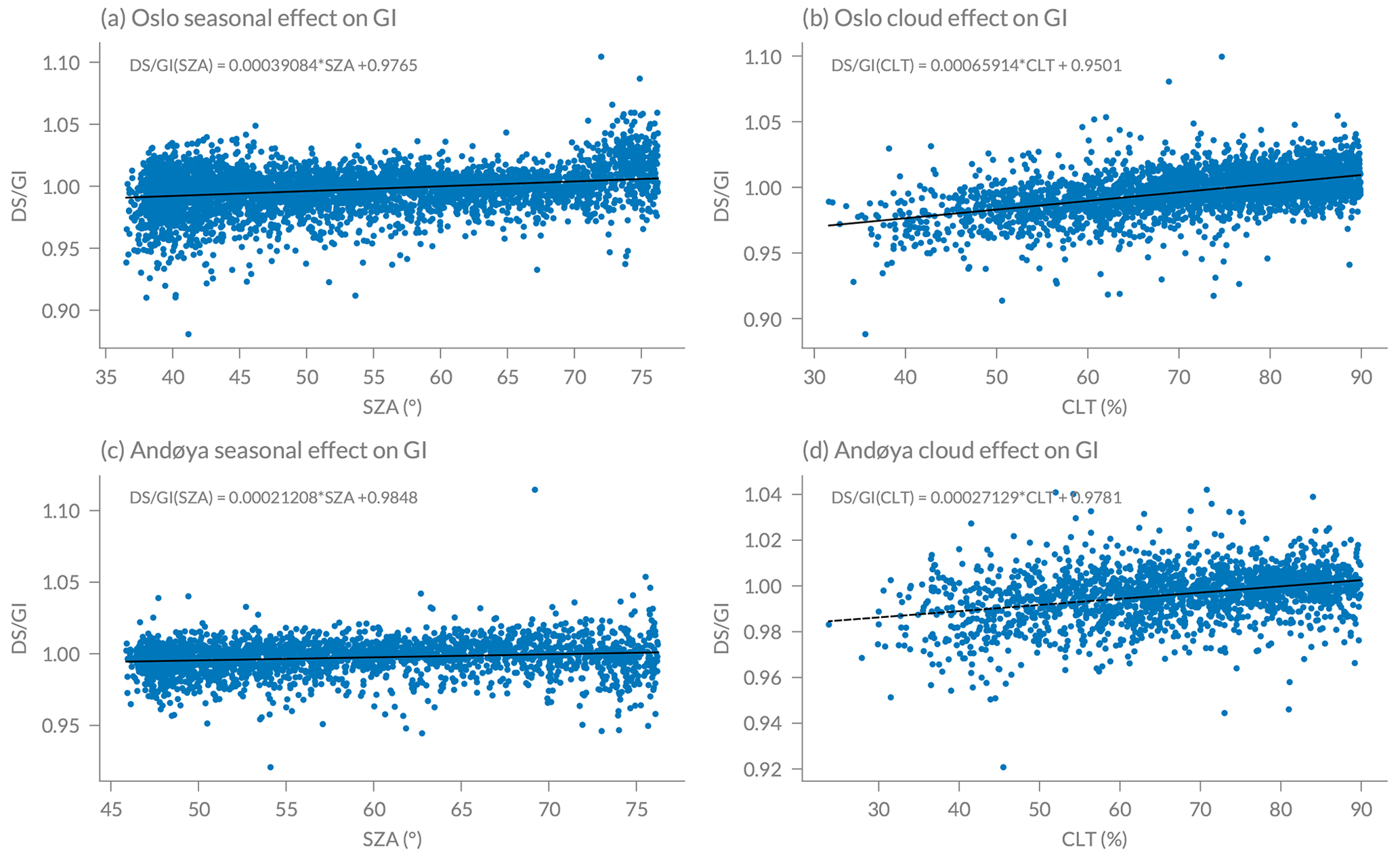
Figure A1 Linear relationships between the DS $/$ GI ratio and (a, c) the solar angle (SZA) as well as (b, d) the cloud transmittance (CLT) for Oslo (1995 to 2020) and Andøya (2000 to 2020).

Table A1 Linear fit between DS $/$ GI ratio and solar zenith angle (SZA) and cloud transmittance (CLT) used for the GI correction in Eq. (A6).

A4 GI validation

Figure A2 shows the comparison of GI daily means with coincident DS data at Oslo and Andøya. On average, we observe an absolute difference between GI and DS of around 1 % at both stations, indicating a good agreement. We observe a slightly higher difference before 2005 at Oslo and after 2015 at Andøya. These episodes coincide with rapid changes in the SL values.

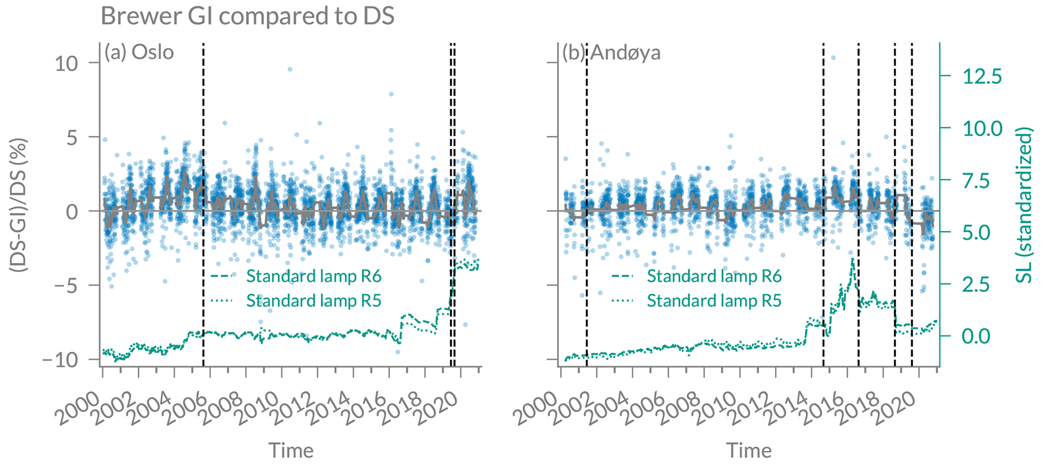
Figure A2 Brewer global irradiance (GI) data compared to DS data at (a) Oslo and (b) Andøya. Data smoothed with a moving mean window of 30 d is shown by the thick grey lines. The right axis shows standard lamp (SL) ratios R5 and R6, standardized to zero mean and standard deviation of 1, smoothed with a moving mean window of 30 d. Vertical dashed lines show dates that were used for GI calibration.

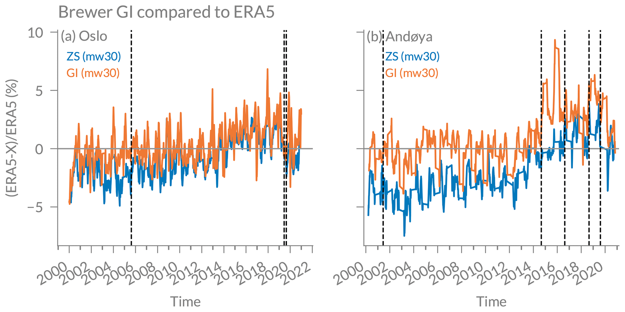
Figure A3 Brewer global irradiance (GI) data and Brewer zenith sky (ZS) data, both compared to ERA5 data at (a) Oslo and (b) Andøya. The time series have been smoothed with a moving mean window of 30 d. Vertical dashed lines show dates that were used for GI calibration.

To validate the GI measurements with independent data, we compared GI daily means also with coincident reanalysis data (ERA5) at both stations (Fig. A3). In addition, we show Brewer data from the zenith sky (ZS) method that is commonly used to retrieve ozone in cloudy conditions (e.g. Fioletov et al., 2011). We observe a good agreement with ERA5 data, with an average absolute difference between ERA5 and GI of 2.3±2.5 % at Andøya and 2.2±2.1 % at Oslo. We further observe that GI measurements agree slightly better with ERA5 than ZS measurements, especially at Andøya (3.3 % difference between ZS and ERA5). Figure A2 also shows the SL measurements for the two SL ratios R5 and R6 and shows large changes in the standard lamp in Andøya between 2015 and 2018. Such irregularities can partly be handled thanks to the regular calibrations and the SL correction in the GI retrieval (see Appendix A2), but we observe larger differences to ERA5 in this period (Fig. A3). However, similar anomalies are observed when comparing ERA5 to GUV data at Andøya, suggesting that ERA5 is also showing a drift from 2015 onwards.

Our results show that the GI method can provide ozone data of higher quality than the commonly used ZS method. The advantage of GI is that it can also be used at high SZA, and the measurement season at high latitudes can therefore be extended in winter months when the sun is low. Furthermore, the GI method is based on physical measurements, whereas the ZS method is normally based on purely statistically derived relationships.

Appendix B: Regression predictors at additional stations

Similar as Fig. 5 for Oslo, the following figures show the monthly contributions of predictors used in the regression model for Andøya (Fig. B1) and Ny-Ålesund (Fig. B2).

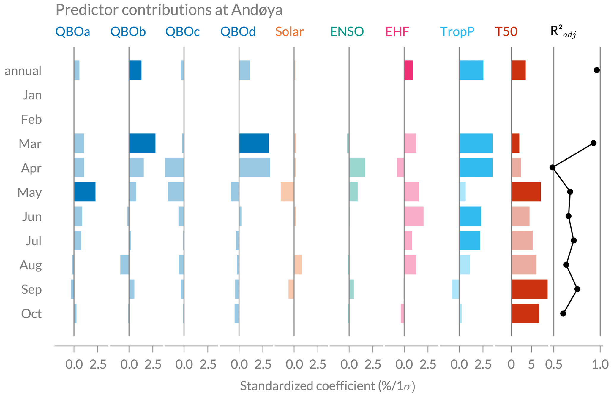
Figure B1 Predictor contribution to the regression fit at Andøya for the annual regression fit and individual monthly fits. The last panel on the right shows the adjusted coefficient of determination ($R_{\mathrm{adj}}^{\mathrm{2}}$) for the annual and all monthly fits. Note that the range of the x axis is different for T50 than for the other predictors.

Figure B2 Same as Fig. B1 but for Ny-Ålesund.