Why is ozone in South Korea and the Seoul metropolitan area so high and increasing?

Surface ozone pollution in South Korea has increased over the past 2 decades, despite efforts to decrease emissions, and is pervasively in exceedance of the maximum daily 8 h average (MDA8) standard of 60 ppb. Here, we investigate the 2015–2019 trends in surface ozone and NO₂ concentrations over South Korea and the Seoul metropolitan area (SMA), focusing on the 90th percentile MDA8 ozone as an air quality metric. We use a random forest algorithm to remove the effect of meteorological variability on the 2015–2019 trends and find an ozone increase of up to 1.5 ppb a⁻¹ in April–May, while NO₂ decreases by 22 %. Global 3-D atmospheric chemistry model simulations including recent chemical updates can successfully simulate surface ozone over South Korea and China as well as the very high free-tropospheric ozone observed above 2 km altitude (mean 75 ppb in May–June) and can reproduce the observed 2015–2019 emission-driven ozone trend over the SMA including its seasonality. Further investigation of the model trend for May, when meteorology-corrected ozone and its increase are the highest, reveals that a decrease in South Korea NO_x emissions is the main driver for the SMA ozone increase. Although this result implies that decreasing volatile organic compound (VOC) emissions is necessary to decrease ozone, we find that ozone would still remain above 80 ppb even if all anthropogenic emissions in South Korea were shut off. China contributes only 8 ppb to this elevated South Korea background, and ship emissions contribute only a few parts per billion. Zeroing out all anthropogenic emissions in East Asia in the model indicates a remarkably high external background of 56 ppb, consistent with the high concentrations observed in the free troposphere, implying that the air quality standard in South Korea is not practically achievable unless this background external to East Asia can be decreased.

1 Introduction

Surface ozone is a severe air quality problem in South Korea and has become steadily worse over the past 2 decades (Gaudel et al., 2018; Yeo and Kim, 2021; Kim et al., 2021). Ozone often exceeds 90 ppb in the Seoul metropolitan area (SMA), where 50 % of South Korea's population is located (Miyazaki et al., 2019). In 2015, Phase 2 of the Seoul Metropolitan Air Quality Control Master Plan established a national standard of 60 ppb for the maximum daily 8 h average (MDA8) ozone concentration (MOE, 2016). However, no monitoring sites have been compliant with this standard in recent years, and ozone has continued to increase (NIER, 2020). Improved understanding of the causes of elevated ozone in South Korea is crucial for developing effective emission control strategies.

Ozone is produced in the troposphere by photochemical oxidation of volatile organic compounds (VOCs) in the presence of nitrogen oxides (NO_x ≡ NO + NO₂). Both VOCs and NO_x have large anthropogenic sources from combustion, and VOCs also have fugitive industrial and residential, as well as biogenic, sources. Effectively reducing ozone concentrations requires knowledge of whether ozone production is NO_x or VOC limited. In the NO_x-limited regime, decreasing NO_x emissions decreases ozone, while decreasing VOC emissions has little effect. In the VOC-limited regime, when NO_x concentrations are very high, decreasing NO_x emissions drives an increase in ozone, while decreasing VOC emissions decreases ozone (Sillman et al., 1990). The Clean Air Policy Support System (CAPSS) bottom-up emission inventory in South Korea reports emission declines of 26 % for NO_x and 25 % for VOCs in Seoul over the 2000–2019 period (https://www.air.go.kr/eng/capss/emission/sido.do?menuId=100, last access: 1 December 2022). Using satellite and surface observations of NO₂, Seo et al. (2021) found that NO_x emissions declined in Seoul by 30 % during the 2015–2019 period, and Bae et al. (2021) found an 18 % decrease for the 2015–2018 period. On the other hand, Bauwens et al. (2022) found an increase in satellite-observed HCHO columns over South Korea by 1 % a⁻¹–2 % a⁻¹ for the 2005–2019 period, which does not support a decrease in VOC emissions.

Ozone concentrations over South Korea depend not only on domestic emissions but also on the background from external sources. The KORUS-AQ (Korea–United States Air Quality) aircraft campaign in May–June 2016 found free-tropospheric concentrations above 2 km altitude frequently exceeding 80 ppb (Miyazaki et al., 2019; Sullivan et al., 2019; Gaubert et al., 2020; Crawford et al., 2021), which would affect surface ozone through subsidence. An obvious source of background ozone is China, where ozone is very high and increasing (Li et al., 2019, 2021) and would be transported to South Korea by westerly winds (Cuesta et al., 2018). But other background sources could also contribute. Lam and Cheung (2022) found that strong transport from the stratosphere can enhance springtime surface ozone by up to 8 ppb in East Asia. Li et al. (2016) estimated from a global model that long-range transport from outside East Asia could contribute 50 %–80 % to annual surface ozone in the Korean Peninsula. Wang et al. (2022) found an increase in free-tropospheric ozone over East Asia of 3.8 to 6.7 ppb per decade over the 1995–2017 period.

The high and increasing ozone over South Korea could thus reflect a combination of decreasing NO_x emissions and/or increasing VOC emissions under VOC-limited conditions for ozone production (Jung et al., 2018), as well as high and increasing background ozone. Here we aim to better understand the factors controlling ozone and its increase in the SMA and more broadly over South Korea during the 2015–2019 period. We focus our analysis on the 90th percentile MDA8 ozone as a robust metric for polluted conditions (Fiore et al., 1998; Sun et al., 2017; Wells et al., 2021). We use a random forest (RF) method (Grange et al., 2018) to correct for the role of meteorology in driving the 2015–2019 ozone trend in the SMA and show that meteorology-corrected ozone is highest in May–June and increases the fastest in April–May, while showing no significant trend in July–August. We find that a 3-D chemical transport model driven by meteorological input from the Goddard Earth Observing System (GEOS-Chem) can successfully capture the magnitude and trends of ozone concentrations, including their seasonality. We use the model to quantify the importance of domestic and different background contributions in driving elevated ozone and its increase over South Korea.

2 AirKorea data and trends, 2015–2019

We use ozone and NO₂ concentrations measured hourly by the AirKorea national air quality network of the South Korea Ministry of Environment (http://www.airkorea.or.kr/web, last access: 3 October 2022). There are 255 sites in South Korea covering the 2015–2019 period including 79 sites in the SMA defined here as the rectilinear domain (37.2–37.8^∘ N, 126.7–127.3^∘ E). Figure 1 shows the maximum monthly 90th percentile MDA8 ozone at the ensemble of AirKorea sites for each year from 2015 to 2019. Ozone rises steadily over that period except for a dip in 2018, reaching 96 ppb in 2019 averaged across all AirKorea sites. High values are spread throughout South Korea, and no site meets the 60 ppb air quality standard. Also shown is the monthly time series of ozone for the SMA. Ozone levels are similar to the rest of South Korea, though they do not show the 2018 dip. The seasonal maximum is in May–August depending on the year.

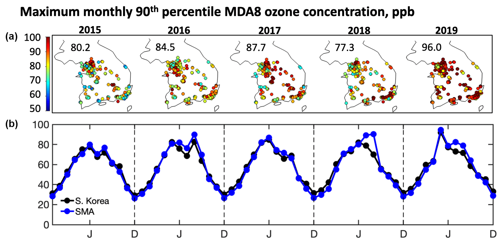
Figure 1 The 90th percentile maximum daily 8 h average (MDA8) ozone concentrations in South Korea for 2015–2019. Panel (a) shows the maximum monthly 90th percentile ozone at individual AirKorea sites. The mean of this statistic across the ensemble of sites is shown inset. Panel (b) shows 90th percentile MDA8 ozone averaged for individual months over sites within the Seoul metropolitan area (SMA; 37.2–37.8^∘ N, 126.7–127.3^∘ E), as well as for all AirKorea sites. Tick marks are for June, and dashed lines are for December. Only sites with over 90 % of observational coverage for the 2015–2019 period are included in this analysis.

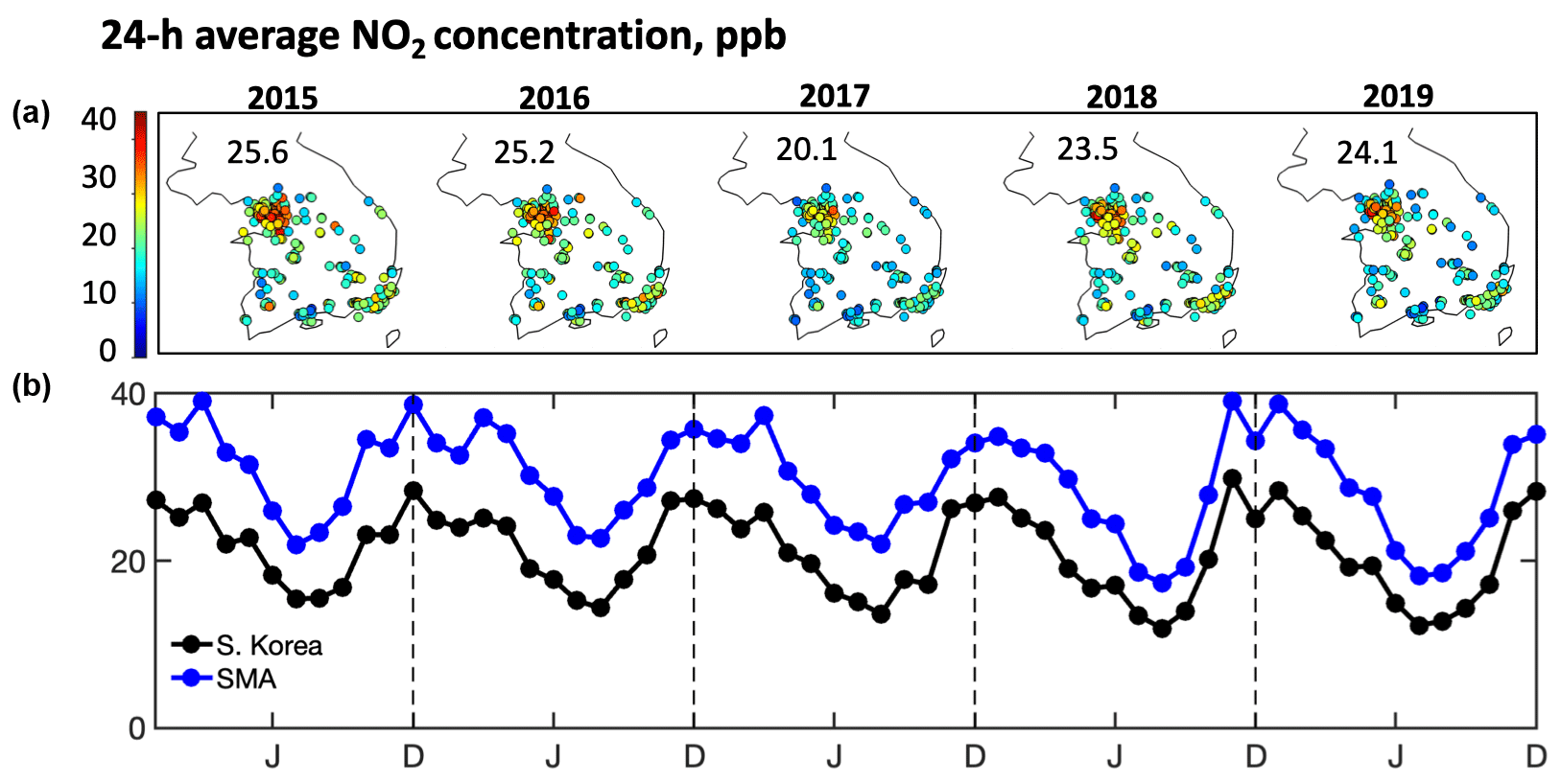
Figure 2 Same as Fig. 1 but for 24 h average annual mean NO₂ concentrations.

Figure 2 shows the annual mean 24 h average NO₂ concentration at the ensemble of AirKorea sites. Concentrations of NO₂ in the SMA are generally 10 ppb higher than averaged across South Korea. NO₂ concentrations peak in winter and are minimum in summer, as observed elsewhere in East Asia, and are mostly driven by longer NO_x lifetime and reduced vertical mixing in winter (Lamsal et al., 2010; Shah et al., 2020; Lin et al., 2019; Kim et al., 2020). There is a decreasing trend over the 2015–2019 period as previously reported by Seo et al. (2021), with this being the case more so in summer than in winter.

3 Meteorological correction of 2015–2019 trends in the SMA

The 2015–2019 trends in ozone and NO₂ concentrations from Figs. 1 and 2 could reflect not only emission trends but also meteorological variability. Here we use a random forest (RF) non-parametric statistical model (Breiman, 2001; Tong et al., 2003) to isolate and remove the effect of meteorological variability for the 79 AirKorea sites in the SMA (Fig. 3). RF is a supervised ensemble machine learning method, where many individual uncorrelated decision trees are fit to the training data to predict an output value, with the average value taken as the best estimate (Breiman, 2001). The RF model was constructed using R “normalweatherr” packages (https://github.com/skgrange/normalweatherr, last access: 17 August 2022; Grange et al., 2018). Hourly meteorological data are from two sites operated by the Korea Meteorological Administration (KMA) within the SMA (https://data.kma.go.kr/data/grnd, last access: 21 June 2022). The RF model is trained to predict the hourly ozone and NO₂ concentrations averaged across the 79 AirKorea sites using the meteorological data averaged for the two KMA sites as well as the time of the day, the day of the year and a long-term linear trend (Unix timestamp). Explanatory variables for the RF algorithm are listed in Table 1. Training of the RF model was conducted on 70 % of the input data, and the other 30 % was withheld as testing data. The number of variables used to grow a tree was set to 3, the minimum node size was 5 and the number of trees within a forest was set to 300. Once trained, the RF model is then used to predict ozone and NO₂ concentrations based on randomly sampled meteorological data, and predictions are aggregated as described below.

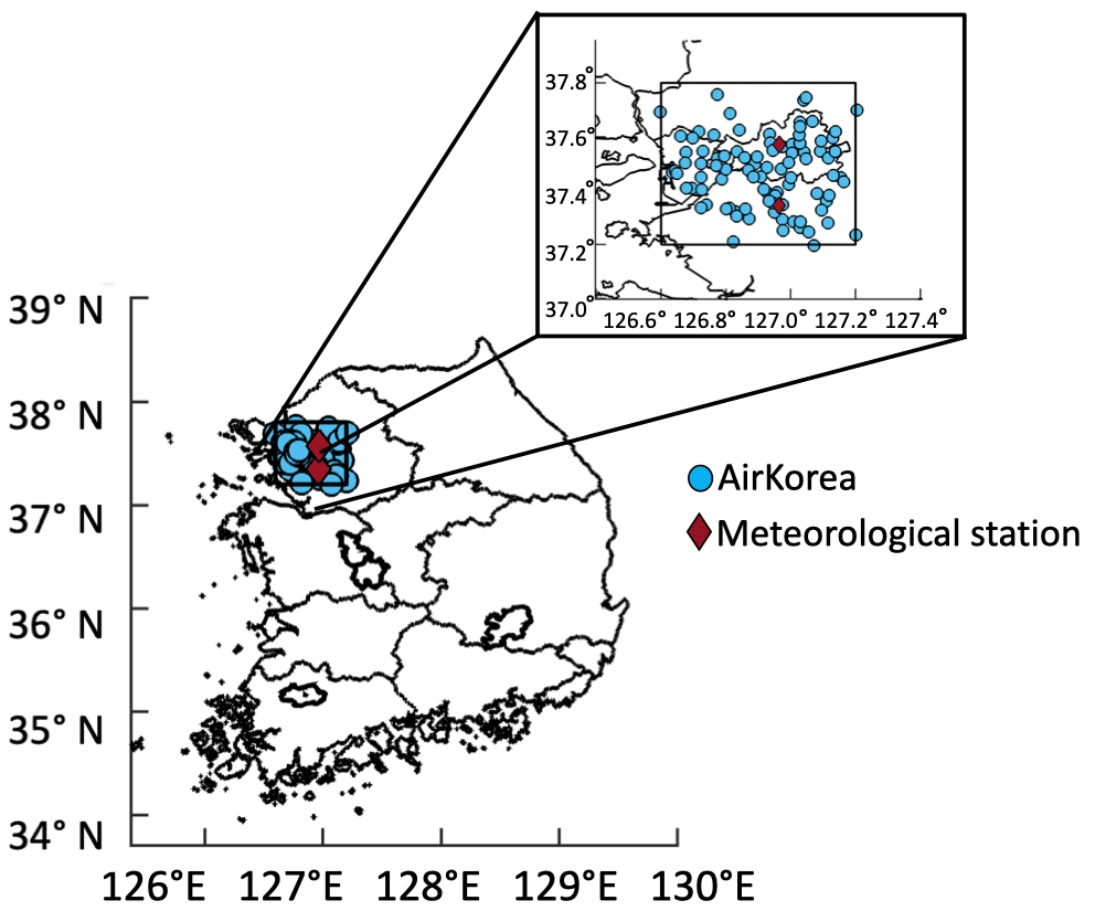
Figure 3 AirKorea monitoring sites in the Seoul metropolitan area (SMA) with hourly ozone and NO₂ concentration data for 2015–2019. Red diamonds show the two meteorological sites in the SMA operated by the Korea Meteorological Administration (https://data.kma.go.kr/data/grnd).

Figure 4 compares observed and predicted hourly concentrations of ozone and NO₂ for the data withheld from training. The RF model shows a strong predictive ability (R=0.93 for ozone, 0.90 for NO₂) with negligible mean bias (0.23 ppb for ozone, 0.01 ppb for NO₂) and a root mean square error (RMSE) of 5.9 ppb for ozone and 6.2 ppb for NO₂. The model has difficulty in capturing the tails of the distribution, which is a well-recognized problem in RF algorithms (Zhang and Lu, 2012; Pendergrass et al., 2022).

Table 1 Random forest predictor variables for hourly ozone and NO₂ concentrations^a.

^a Hourly explanatory variables in the random forest (RF) model fitted to hourly ozone and NO₂ concentrations averaged across 79 AirKorea sites in the Seoul metropolitan area (SMA) for 2015–2019. ^b Meteorological data are from the two SMA stations for synoptic meteorological observation (https://data.kma.go.kr/data/grnd) located at Gwanaksan (37.345^∘ N, 126.975^∘ E) and in Seoul (37.585^∘ N, 126.980^∘ E). Data are averaged across the two stations for input to the RF model. ^c Day of the year, used as a seasonal term. ^d Used as a linear-trend term.

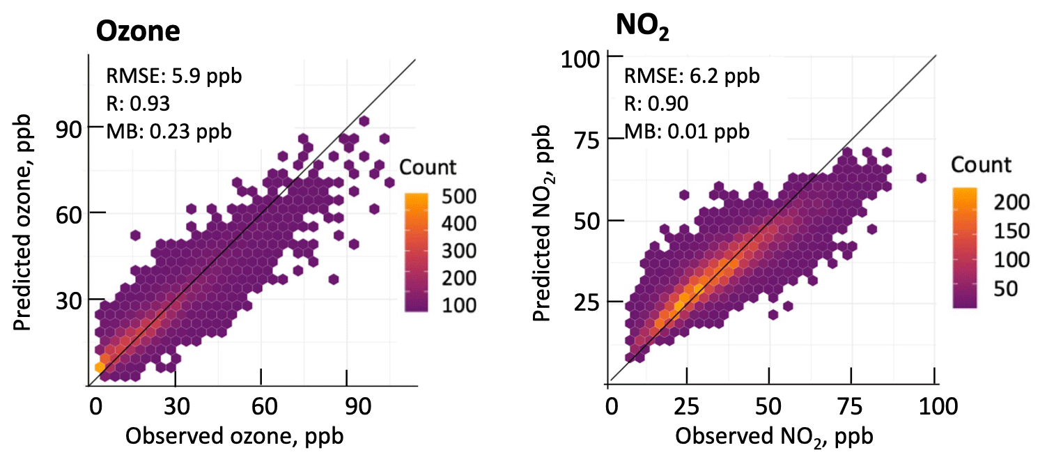
Figure 4 Performance of the random forest (RF) model in fitting 2015–2019 hourly ozone and NO₂ concentrations in the Seoul metropolitan area (SMA). The RF model is trained on hourly concentrations averaged across 79 AirKorea monitoring sites in the SMA (Fig. 3). The figure compares predicted and observed values for the 30 % of data withheld from training. Comparison statistics are shown inset including the root mean square error (RMSE), correlation coefficient (R) and mean bias (MB). Also shown are the 1 : 1 lines. Count refers to the number of data points within a given (ozone, NO₂) data bin (individual symbol).

The top predictors in the RF fit for ozone are the temperature, day of the year, relative humidity, hour of the day and wind speed, in that order, consistent with previous studies for urban areas (Sillman and Samson, 1995; Jacob and Winner, 2009; Li et al., 2020). The top predictors for NO₂ are the wind speed, day of the year, temperature, hour of the day and surface pressure, again consistent with previous studies (Liu et al., 2020; Richmond-Bryant et al., 2018).

We use the RF model to remove the effect of meteorological variability in driving the 2015–2019 ozone and NO₂ trends by following the technique outlined in Vu et al. (2019). Meteorological variables for a specific hour and date in the input dataset are replaced by randomly selecting weather data over the entire study period (2015–2019) at that hour of the day but for a different day of the year within a 4-week period (2 weeks before to 2 weeks after the selected date). This process is repeated 1000 times, and the resulting 1000 RF predictions of ozone and NO₂ for that hour and date are then averaged to produce meteorology-corrected concentrations from which we recalculate MDA8 ozone and 24 h averaged NO₂ to infer 2015–2019 emission-driven trends.

4 Emission-driven trends in ozone and NO₂ concentrations in the SMA, 2015–2019

Figure 5 shows the observed and meteorology-corrected trends of monthly 90th percentile MDA8 ozone concentrations in the SMA from 2015 to 2019. The observations show peak increase in May but a highly variable trend from month to month driven in part by interannual meteorological variability. The meteorology-corrected data show a much smoother behavior with a broad springtime (March–May) maximum in the increasing ozone trend and a decreasing trend in August. Meteorology-corrected ozone is highest in May–June for all years. The 2015–2019 trend in meteorology-corrected 90th percentile ozone is 0.7, 1.4 and 0.4 ppb a⁻¹ for winter, spring and fall. The overall trend for summer is not statistically significant, but the trend for June alone is 0.9 ppb a⁻¹. This seasonality of ozone trends in the SMA from 2015 to 2019 is consistent with the 2000–2014 results of Jung et al. (2018), who reported a maximum springtime ozone increase in South Korea and an advancement of the ozone season by 2.1 d a⁻¹. Similar seasonality in the ozone trend has been reported for the North China Plain (Li et al., 2021), showing a 2-fold increase in May ozone exceedances above the 75 ppb standard from 2014 to 2019. Ozone production is most likely to be NO_x limited in summer when solar radiation and biogenic emissions are highest and VOC limited in spring and fall (Jacob et al., 1995); thus the seasonality of the trend is consistent with VOC-limited conditions.

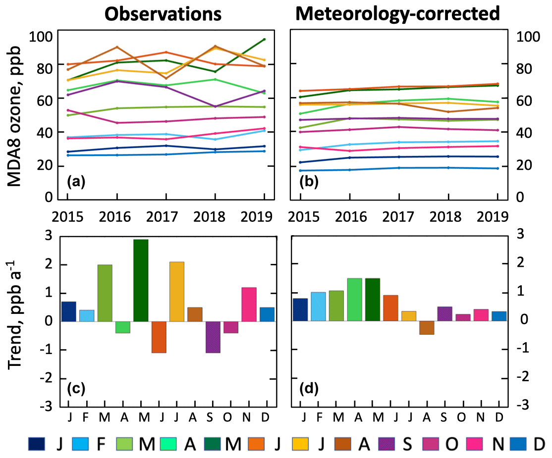
Figure 5 The 2015–2019 trends in monthly 90th percentile MDA8 ozone averaged across the 79 AirKorea sites in the Seoul metropolitan area (SMA). Panels (a) and (c) show the observed trends for individual months, and panels (b) and (d) show meteorology-corrected trends. Panels (c) and (d) show the 2015–2019 slopes for individual months obtained by ordinary least-squares regressions of the data in panels (a) and (b).

Figure 6 Same as Fig. 5 but for 24 h average NO₂ concentrations. Trends are shown in percent per annum relative to the 2015–2019 mean.

Figure 6 is the same as Fig. 5 but for 24 h average NO₂ concentrations. The observations show a >2 % a⁻¹ decrease in all months except November–February. The meteorology-corrected data show a consistent 5.6 % a⁻¹ decrease in March–October, or 22 % over the 4 years, and a consistent but weaker 1.5 % a⁻¹ decrease in November–February. This is consistent with findings from Bae et al. (2021), who reported a 4.4 % a⁻¹ decline in annual mean NO₂ in the SMA for 2015–2018 using surface and satellite observations. Declining NO₂ in the SMA can be attributed to policies to decrease vehicular NO_x emissions (Kim and Lee, 2018). The weaker decline in winter is consistent with findings from Seo et al. (2021), who found that surface NO₂ concentrations in the SMA in 2015–2019 declined by 5.3 % a⁻¹ during the time of the morning commute for the ozone season but only by 2.6 % a⁻¹ for the non-ozone season. The weaker response of NO₂ to reduced NO_x emissions in winter could be due to ozone titration by emitted NO, which would take place most systematically at night but also extend to daytime if the ozone supply is weak. We find that in November–February the decline in NO₂ during midday (11:00–15:00 LT) is 2.4 % a⁻¹, greater than twice that at night (23:00–03:00 LT), consistent with ozone titration. For the GEOS-Chem simulations in the following sections we will assume a 22 % decrease in NO_x emissions from 2015 to 2019.

5 GEOS-Chem simulation

We use the GEOS-Chem chemical transport model version 13.3.4 (http://geos-chem.org, last access: 27 October 2022) to interpret the observed ozone and its 2015–2019 trend in the SMA and more broadly in South Korea, including influences from China and the global background. GEOS-Chem has been applied previously in South Korea to investigate ozone production efficiency (Oak et al., 2019), the factors determining ozone seasonality (Lee and Park, 2022) and the photochemical environment for ozone production (Yang et al., 2023). Park et al. (2021) previously found that GEOS-Chem version 12.7.2 underestimated free-tropospheric ozone over South Korea by 20–30 ppb. Addition of detailed aromatic chemistry in version 13.3.4 (Bates et al., 2021) was subsequently found to increase net ozone production over South Korea by 37 % (Oak et al., 2019). Here we also add particulate nitrate photolysis and suppression of sea salt aerosol debromination to the model following Shah et al. (2023), and as we will see this largely corrects the remaining model ozone bias over East Asia.

We use a nested-grid version of GEOS-Chem driven by MERRA-2-assimilated (Modern-Era Retrospective analysis for Research and Applications) meteorological data with a horizontal resolution of 0.5^∘ × 0.625^∘ over East Asia (25–50^∘ N, 105–140^∘ E; domain of Fig. 7). Chemical boundary conditions at the edges of the nested domain are updated every 3 h from a global simulation with 4^∘ × 5^∘ resolution. We conduct a full-year simulation for 2016 with 6 months of initialization. Global anthropogenic emissions are from the Community Emissions Data System (CEDS) global inventory (Hoesly et al., 2018) and are superseded with regional emission inventories for South Korea (KORUSv5, http://aisl.konkuk.ac.kr, last access: 13 May 2022) and China (Multi-resolution Emission Inventory model for Climate and air pollution research, MEIC; Zheng et al., 2018). Natural emissions include NO_x from lightning (Murray et al., 2012) and soil (Hudman et al., 2012), MEGANv2 biogenic volatile organic compounds (VOCs) (Guenther et al., 2012), dust (Meng et al., 2021), and sea salt (Jaeglé et al., 2011). Open-fire emissions are from the Global Fire Emissions Database version 4 (GFED4; van der Werf et al., 2017).

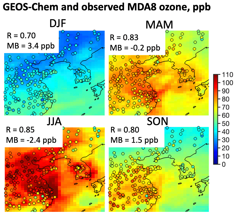
Figure 7 Monthly 90th percentile MDA8 ozone over South Korea and China for different seasons in 2016. GEOS-Chem model results for each season (background contours) are compared to AirKorea and MEE network observations (symbols); 50 % of network sites have been culled randomly for visualization purposes. The GEOS-Chem correlation coefficient (R) and mean bias (MB) relative to observations are shown inset. DJF: December–January–February, MAM: March–April–May, JJA: June–July–August, SON: September–October–November.

Ships are a relatively large source of NO_x in East Asia. The standard GEOS-Chem model includes pre-processing of ship emissions with the PARAmeterization of emitted NO_x (PARANOX) algorithm (Vinken et al., 2011) to account for the non-linear chemistry occurring during the dispersion of ship exhaust plumes. PARANOX is a plume-in-grid formulation where ship emissions are aged chemically for 5 h before being released into the model grid. This greatly reduces the ozone yield from ship NO_x emissions, which would otherwise be diluted by the model in a relatively clean environment where the ozone production efficiency is very high. PARANOX was intended for global model simulations with a grid resolution of hundreds of kilometers (Holmes et al., 2014), and its application to higher-resolution simulations is questionable, particularly over East Asia, where the maritime environment is highly polluted (Cuesta et al., 2018; Peterson et al., 2019; Jung et al., 2022). Here we disable PARANOX for the nested simulation and find that this increases ozone over the Yellow Sea in May by 1 ppb on average.

We evaluate our GEOS-Chem simulation for 2016 with MDA8 ozone observations from the AirKorea network in South Korea and the Ministry of Ecology and Environment (MEE) monitoring network in China (http://data.epmap.org/page/index, last access: 9 July 2022). Observations of seasonal mean 90th percentile MDA8 ozone overlaid on our GEOS-Chem simulation are shown in Fig. 7. There is good agreement between GEOS-Chem and observations in all seasons, with a spatial correlation coefficient R>0.7 and a mean bias <4 ppb.

We evaluated GEOS-Chem's ability to reproduce the seasonal cycle of ozone in the three megacity clusters of the Seoul metropolitan area (SMA), Beijing–Tianjin–Hebei (BTH) and the Yangtze River Delta (YRD). Figure 8 shows the monthly 90th percentile MDA8 ozone for 2016 averaged over all network sites in each cluster. The simulated seasonal cycle is consistent with observations (R>0.95 and mean bias <6.0 ppb).

Figure 8 Seasonal variation in monthly 90th percentile MDA8 ozone in three megacity clusters in 2016. The clusters are the Seoul metropolitan area (SMA; 37.2–37.8^∘ N, 126.7–127.3^∘ E), the Yangtze River Delta (YRD; 30–33^∘ N, 118–122^∘ E) and Beijing–Tianjin–Hebei (BTH; 37–41^∘ N, 114–118^∘ E). GEOS-Chem results are compared to observations, and the corresponding root mean square error (RMSE) and mean bias (MB) are shown inset. The 90th percentiles are computed from the time series of spatial mean concentrations for each cluster, with GEOS-Chem sampled at the network sites.

May is of particular interest in the SMA because this is when ozone and its increasing trend are highest in the meteorology-corrected data (Fig. 5). Previous model comparisons to extensive vertical profiles taken during the KORUS-AQ aircraft campaign over South Korea in May–June 2016 showed large underestimates, with GEOS-Chem version 12.7.2 being too low by 20–30 ppb (Park et al., 2021). The model updates described above largely correct this underestimate (Yang et al., 2023). Figure 9 compares our simulated GEOS-Chem ozone profile to the mean of 15 ozonesonde observations over Olympic Park in Seoul taken during the KORUS-AQ campaign on DC-8 flight observation days (15 profiles in total). Our simulation has a low bias of only 5.4 ppb in the free troposphere.

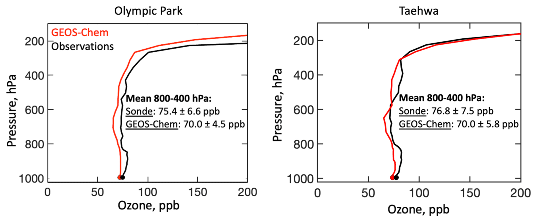
Figure 9 Mean vertical ozone profile over Olympic Park (37.522^∘ N, 127.124^∘ E) and Taehwa Research Forest (37.312^∘ N, 127.310^∘ E) in Seoul during KORUS-AQ (May–June 2016). Observations from Olympic Park and Taehwa are from 15 and 42 ozonesondes, respectively. Ozonesondes were launched between 13:00 and 14:00 local time on KORUS-AQ flight days. GEOS-Chem model results are sampled at the observation times. The circles show the surface ozone concentrations from GEOS-Chem and the AirKorea site in the closest proximity.

To investigate and diagnose the ability of GEOS-Chem to reproduce the observed 2015–2019 ozone trend in the SMA, we performed simulations with 2016 meteorology (January–December 2016) and perturbed emissions in China and South Korea for 2015 and 2019 to simulate the 2015–2019 trend. The sensitivity simulations used 6 months of initialization. China emissions in 2015 are from MEIC (Zheng et al., 2018), but MEIC does not extend beyond 2017. Following Li et al. (2021), we scaled 2017 MEIC emissions to 2019 based on observed MEE network trends. Overall, emissions in China declined from 2015 to 2019 by 16 % for NO_x, 50 % for SO₂, 23 % for CO and 32 % for primary PM_2.5, with flat VOC emissions (Li et al., 2021). Anthropogenic emissions for South Korea in 2015 are taken from the KORUSv5 inventory (http://aisl.konkuk.ac.kr). For 2019 we decrease NO_x emissions in South Korea by 22 % (Sect. 4) and apply no other changes to South Korea emissions, including VOCs for which emission trends are not clear, as mentioned in the Introduction. We also do not apply trends to ship emissions.

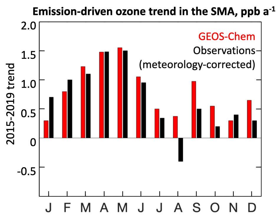
Figure 10 Emission-driven trends in 90th percentile MDA8 ozone from 2015 to 2019 in the Seoul metropolitan area (SMA) for individual months. The observed meteorology-corrected trend is as shown in Fig. 5. The modeled trend is obtained by subtraction of results from simulations with 2015 and 2019 emissions, both using the same 2016 meteorology.

Figure 10 shows the emission-driven trends of 90th percentile MDA8 ozone from 2015 to 2019 in the SMA for both meteorology-corrected observations (data from Fig. 5) and GEOS-Chem in individual months. The model trend is obtained by the subtraction of results from simulations with 2015 and 2019 emissions, both using the same 2016 meteorology. GEOS-Chem reproduces the general magnitude and seasonality of the observed trend. It reproduces in particular the April–May maximum in the trend.

6 Attribution of ozone and its 2015–2019 trend over South Korea

We exploit the success of GEOS-Chem in simulating ozone over East Asia and its trend over the SMA to investigate the causes. We focus on May, where both ozone concentrations and the increasing trend in the meteorology-corrected data for the SMA are the highest. In addition to the baseline simulation described in Sect. 5, we also conduct sensitivity simulations for both emission years to isolate the effects of anthropogenic emissions from South Korea, China, ships and East Asia as a whole by zeroing the corresponding emissions including NO_x, VOCs, CO and PM_2.5. The same global boundary conditions described above are used for each of these cases, with 6 months of initialization.

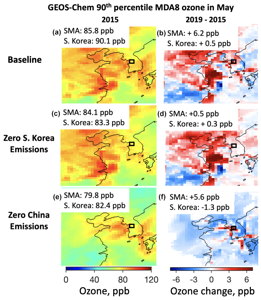
Figure 11 Emission-driven ozone changes over East Asia from 2015 to 2019 in GEOS-Chem. Results show the 90th percentile MDA8 ozone for May simulated by GEOS-Chem using 2015 emissions, as well as the difference using 2019 emissions, both for the same meteorological year. Panels (a) and (b) show the baseline simulation described and evaluated with observations in Sect. 5. Panels (c)–(f) show sensitivity simulations with zero anthropogenic emissions in South Korea and China, respectively. Spatially averaged values for the Seoul metropolitan area (SMA) and South Korea are given inset.

Figure 11 shows the distribution of simulated 90th percentile MDA8 ozone for May using 2015 emissions, the difference when using 2019 emissions, and the contributions from South Korea and China as determined from the sensitivity simulations with the corresponding emissions shut off. The 2015 values in the baseline simulation average 85.8 ppb in the SMA and 90.1 ppb for all of South Korea, and the 2019–2015 difference averages +6.2 ppb for the SMA, while southern parts of the country show decreases. Zeroing out South Korea emissions has remarkably little effect on SMA concentrations, which remain at 84.1 ppb for 2015, though the 2015–2019 trend is now near zero. Zeroing out China emissions decreases SMA ozone concentrations to 79.8 ppb, but the 2015–2019 increase remains at 5.6 ppb. We conclude that the 2015–2019 ozone increase in the SMA can be attributed to the decrease in domestic NO_x emissions under VOC-limited conditions. When emissions from China are zeroed out, we find a 6 ppb ozone decrease in the SMA and an 8 ppb decrease in South Korea as a whole compared to the baseline simulation. The 2015–2019 ozone trend over the SMA is affected by less than 1 ppb, confirming that this trend is mainly driven by domestic emission changes.

A notable result is that ozone levels over South Korea remain very high at about 80 ppb even when emissions from either South Korea or China are totally shut off. Lee and Park (2022) previously found with GEOS-Chem that surface ozone over South Korea in April hardly changes when domestic emissions are shut off, and here we find that zeroing China emissions also has only a modest effect over South Korea. This resilience is indicative of a major contribution to ozone pollution from the northern midlatitude background external to East Asia.

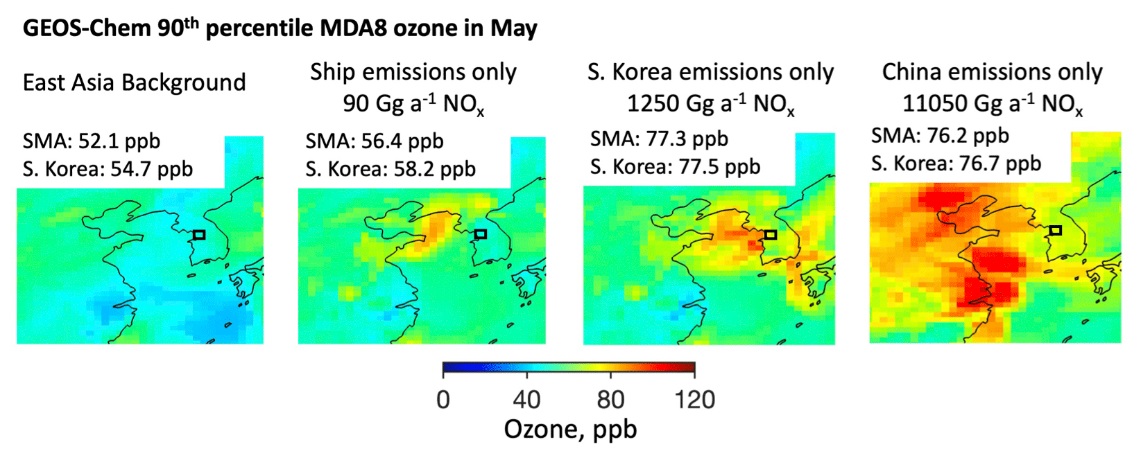
Figure 12 East Asia background ozone and individual enhancements due to anthropogenic emissions from ships in the Yellow Sea (north of 30.5^∘ N), South Korea and China. Results show the monthly mean 90th percentile MDA8 ozone for May simulated by GEOS-Chem for meteorological year 2016.

Figure 12 further explores the role of this East Asia background in a simulation with anthropogenic emissions shut off throughout the nested model domain. The 90th percentile MDA8 ozone drops to 55 ppb in South Korea, meeting the 60 ppb standard but still extremely high and indicating that even low anthropogenic emissions would cause ozone to rise above the standard. This high East Asia background affects northern China even more. Lam and Cheung (2022) previously found with GEOS-Chem that the mean MDA8 background ozone over China in April is 53 ppb, and we find here that the 90th percentile over northern China reaches 70 ppb. This East Asia background ozone is much higher than the corresponding North America background of 20–40 ppb previously reported in studies of US ozone pollution (Fiore et al., 2003; Zhang et al., 2011; Emery et al., 2012; Jaffe et al., 2018). Such a high East Asia background is reflected in the observation of 75 ppb ozone in the free troposphere (Fig. 9), while comparable ozonesonde observations over the western US in spring show mean values of 60 ppb (Zhang et al., 2011). Satellite observations of free-tropospheric ozone also show particularly high values over East Asia (Hu et al., 2017; Gaudel et al., 2018). High free-tropospheric ozone over East Asia in spring could reflect regional downwelling from the stratosphere associated with cyclogenesis (Hwang et al., 2007). It could also reflect the observed rise in free-tropospheric ozone at northern midlatitudes and particularly over East Asia in recent decades (Gaudel et al., 2018; Lee et al., 2021; Wang et al., 2022), which could possibly be due to increasing emissions in India and the Middle East (Anwar et al., 2021; Ding et al., 2022; Anenberg et al., 2022). We find from analysis of sonde observations at Pohang, South Korea; Hong Kong SAR, China; and Tateno, Japan (https://woudc.org/data/dataset_info.php?id=ozonesonde, last access: 5 August 2022), no significant trend in free-tropospheric ozone over South Korea during 2015–2019, meaning that the background is not responsible for the observed increase in surface ozone over that period. Domestic emissions are likely responsible, as discussed above.

Additional panels in Fig. 12 show the enhancement of ozone above the East Asia background due to emissions from the Yellow Sea (ships), South Korea and China. Emissions from ships in the Yellow Sea enhance 90th percentile MDA8 ozone over South Korea by only a few parts per billion, although they can drive ozone concentrations over the ocean in excess of 90 ppb. Despite ship traffic in the Yellow Sea being intense, the NO_x emissions are still low relative to continental emissions. Emissions from South Korea alone push ozone to almost 80 ppb over South Korea, with even larger increases over the surrounding oceans reflecting VOC-limited conditions over land. In this way, emissions in South Korea push ozone in the Shandong Peninsula in China to over 80 ppb. Emissions in China have an effect on ozone over South Korea comparable to domestic emissions.

7 Conclusions

We examined the factors controlling the high and increasing surface ozone concentrations over South Korea and particularly in the Seoul metropolitan area (SMA). Ozone in South Korea has risen steadily over the past 2 decades and is everywhere far in excess of the 60 ppb air quality standard set by the government of South Korea in 2015. Improved understanding of the causes of elevated ozone in South Korea is critical for developing effective emission control strategies.

We find a continuation of the multidecadal increase in surface ozone in South Korea. Analysis of 2015–2019 data from the AirKorea network of air quality monitoring sites shows elevated ozone throughout South Korea, with 90th percentile ozone averaged across all sites exceeding 75 ppb every year and increasing over the period. NO₂ concentrations also measured at AirKorea sites are typically >10 ppb higher in the SMA than elsewhere, with maximum concentrations in winter and a decrease over the 2015–2019 period.

We used a random forest (RF) non-parametric statistical model to isolate and remove the effect of meteorological variability on 2015–2019 ozone and NO₂ trends in the SMA. Meteorology-corrected ozone is highest in May–June for all years and increases at the fastest rate of 1.5 ppb a⁻¹ in April–May. Meteorology-corrected NO₂ is highest during November–March and lowest in July–August. During the ozone season of March–October, NO₂ shows a consistent decline of 5.6 % a⁻¹ over the 2015–2019 period, whereas in winter the decline is lower at 1.3 % a⁻¹. The March–October trend in NO₂ concentrations suggests that NO_x emissions declined by 22 % from 2015 to 2019.

We used the GEOS-Chem chemical transport model to interpret the elevated ozone and its 2015–2019 trend in SMA and more broadly in South Korea, including influences from China and the global background. We improved on previous versions of the model, which substantially underestimated tropospheric ozone over South Korea, through the addition of detailed aromatic chemistry in version 13.3.4 (Bates et al., 2021), the removal of sea salt aerosol debromination and the addition of particulate nitrate photolysis (Shah et al., 2023). The resulting model can reproduce the seasonality and spatial distribution of surface ozone in South Korea and China without significant bias. It reproduces the high free-tropospheric ozone concentrations observed over Seoul during the KORUS-AQ campaign in May–June 2016 (75 ± 7 ppb) with a bias that is only 5 ppb too low. Implementing in the model the 2015–2019 emission decreases in South Korea and China reproduces the observed seasonality and magnitude of the meteorology-corrected ozone trend over the SMA.

We used GEOS-Chem sensitivity simulations for emission years 2015 and 2019 to better understand the factors contributing to elevated ozone in the SMA and South Korea, focusing on May, when meteorology-corrected ozone and its increase are the highest. We find that the 2015–2019 ozone increase in the SMA can be explained by the 22 % decrease in surface NO₂ concentrations, which act as a proxy for declining NO_x emissions, reflecting the VOC-limited conditions for ozone production. We also find that emissions in China and South Korea contribute equally to elevated ozone over South Korea, while ships only contribute a small amount. VOC emission reductions would be expected to decrease ozone in South Korea, but we find that concentrations remain over 80 ppb even if all anthropogenic emissions from South Korea or from China are zeroed out. The East Asia background, defined by zeroing out all anthropogenic emissions over East Asia, is very high at 55 ppb, implying that the 60 ppb air quality standard in South Korea is not achievable without addressing the origin of this elevated background.