the Creative Commons Attribution 4.0 License.
the Creative Commons Attribution 4.0 License.
 | 24 Mar 2023
Technical note: Unsupervised classification of ozone profiles in UKESM1
Daniel C. Jones
Yan Wu
James Keeble
Alexander T. Archibald
The vertical distribution of ozone in the atmosphere, which features complex spatial and temporal variability set by a balance of production, loss, and advection, is relevant for both surface air pollution and climate via its role in radiative forcing. At present, the way in which regions of coherent ozone structure are defined relies on somewhat arbitrarily drawn boundaries. Here we consider a more general, data-driven method for defining coherent regimes of ozone structure. We apply an unsupervised classification technique called Gaussian mixture modeling (GMM), which represents the underlying distribution of ozone profiles as a linear combination of multi-dimensional Gaussian functions. In doing so, GMM identifies coherent groups or subpopulations of the ozone profile distribution. As a proof-of-concept study, we apply GMM to ozone profiles from three subsets of the UKESM1 coupled climate model runs carried out for CMIP6: specifically, the seasonal mean of a historical subset (2009–2014) and two subsets from two different future climate projections (i.e., SSP1-2.6 and SSP5-8.5). Despite not being given any spatiotemporal information, GMM identifies several spatially coherent regions of ozone structure. Using a combination of statistical guidance and post hoc judgment, we select a six-class representation of global ozone, consisting of two tropical classes and four mid-to-high-latitude classes. The tropical classes feature a relatively high-altitude tropopause, while the higher-latitude classes feature a lower-altitude tropopause and low values of tropospheric ozone, as expected based on broad patterns observed in the atmosphere. Both of the future projections feature lower ozone concentrations at 850 hPa than the historical benchmark, with signatures of ozone hole recovery. We find that the area occupied by the tropical classes is expanded in both future projections, which are most prominent during austral summer. Our results suggest that GMM may be a useful method for identifying coherent ozone regimes, particularly in the context of model analysis.
- Article
(5314 KB) - Full-text XML
- BibTeX
- EndNote


Earth's atmospheric ozone distribution is a topic of interest because of its effect on climate and its role in protecting surface-dwelling organisms from harmful ultraviolet radiation (Newman and Todara, 2003; Monks et al., 2015). The distribution of ozone varies both vertically and horizontally. Nearly 90 % of ozone is found in the stratosphere, the layer of the atmosphere between 10–50 km, while 10 % is found in the troposphere, the atmospheric layer extending from the surface to 10 km. Stratospheric ozone protects surface-dwelling life by reducing the number of high-energy photons reaching the surface, which would otherwise lead to high occurrences of skin cancer, cataracts, and impaired immune systems (Newman and Todara, 2003; Monks et al., 2009). In contrast, near-surface tropospheric ozone poses a threat to human health as it is a pollutant (Monks et al., 2015).
The spatial variation in ozone is driven by complex atmospheric processes. Unlike many of the important trace gas species studied in the atmosphere, ozone is not directly emitted from natural or anthropogenic sources. Instead, atmospheric ozone concentrations are controlled by chemical, radiative, and dynamical processes that operate on a range of timescales. Adding further complication is the fact that these processes vary significantly with altitude. In the stratosphere, gas-phase photochemical reactions involving oxygen produce ozone (Chapman, 1930), while it is destroyed through reactions involving chlorine, nitrogen, hydrogen, and bromine radical species (Bates and Nicolet, 1950; Crutzen, 1970; Johnston, 1971; Molina and Rowland, 1974; Cicerone et al., 1974). In contrast, tropospheric ozone is produced through photochemical oxidation of ozone precursors such as carbon monoxide (CO), methane (CH4), and non-methane volatile organic compounds (NMVOCs) in the presence of nitrogen oxides (NO and NO2). Similarly, transport processes differ between the stratosphere and troposphere. Because of these different processes, understanding patterns in the vertical distribution of ozone remains a challenge (Monks et al., 2015). These ozone precursors can be transported far downwind of their source locations (Chameides et al., 1992; Monks et al., 2009).
Not only are there significant differences in the processes controlling local ozone mixing ratios at different altitudes, but these processes also respond differently to changes in atmospheric composition and global climate. Past changes in anthropogenic emissions, biomass burning, and lightning have all contributed to increased emissions of ozone precursors and increased tropospheric ozone (Griffiths et al., 2021; Jaffe and Wigder, 2012; Monks et al., 2015; Laban et al., 2018). In contrast, emissions of halogenated ozone-depleting substances (ODSs) at the end of the 20th century led to significant decreases in stratospheric ozone concentrations and the formation of the ozone hole (Keeble et al., 2021). Future projections of ozone concentrations are dependent on assumptions made about greenhouse gas, ozone precursor, and halogenated ODS emissions, and these changes may work against each other. For example, stratospheric ozone mixing ratios are expected to increase in the coming decades as ODS levels decline. However, an acceleration of the Brewer–Dobson circulation (BDC) associated with increasing greenhouse gas concentrations may lead to reductions in lower tropical stratospheric ozone mixing ratios (Eyring et al., 2013; Meul et al., 2016; Keeble et al., 2017), while increasing the transport of ozone into the midlatitude troposphere. Because of these complex interactions, understanding future changes in the vertical distribution of ozone requires simulations performed by complex models (Banerjee et al., 2016; Meul et al., 2018).
Because of this complexity, chemistry–climate and Earth system models are often used to explore changes in atmospheric ozone. A key component in this evaluation is the comparison of ozone derived from different models and/or from different scenarios in the same model (Griffiths et al., 2021; Keeble et al., 2021). Often this is done at the global scale, but if regional comparisons are made, this is often done by averaging ozone profiles over set latitude ranges. However, owing to the complex, spatially heterogeneous processes controlling the distribution of ozone described above, this is a poor method for identifying regions with similar profiles. As climate and ozone mixing ratios change in the future, the boundaries between ozone profiles with similar characteristics might be expected to move. This feature would not be captured by averaging profiles over fixed latitude ranges. In this work, in order to address this limitation in latitude-based averaging methods, we describe the vertical ozone structure with an unsupervised classification method that groups profiles into classes based on their similarity.
Clustering techniques have already been used in ozone concentration studies for understanding long-term variability. Boleti et al. (2020) have applied a multidimensional clustering technique to understand the long-term trend of ozone. Diab et al. (2004) used a six-cluster analysis which resulted in distinct clusters of “background” and “polluted” with below- and above-ozone mixing ratios from over 100 ozonesonde profiles launched from a subtropical Southern Hemisphere Additional Ozonesondes (SHADOZ) (Thompson et al., 2003) site, Irene, South Africa. Jensen et al. (2012) performed a cluster analysis named self-organizing maps (SOMs) (Kohonen, 2012) on over 900 tropical ozonesonde profiles. Their findings with four-cluster results were similar to Diab et al. (2004). Both studies showed that the seasonal influences of biomass burning and convection dominate ozone variability. Stauffer et al. (2016) documented the influence of meteorological conditions on the shape of the ozone profile from the troposphere to the lower stratosphere by applying the SOM clustering technique to ozonesonde data from specific Northern Hemisphere midlatitude geographical regions. Later they expanded the study for global ozonesonde sites to show the variation in ozone profile clusters for various regions and how they vary based on meteorology and chemistry depending on latitude (Stauffer et al., 2018).
In our study, we adopt a Gaussian mixture modeling (GMM) approach, an automated, robust, and standardized unsupervised classification technique that has previously been applied to ocean structure and dynamics (Bishop, 2006; Maze et al., 2017; Jones et al., 2019; Sonnewald et al., 2019; Rosso et al., 2020). GMM does not use any latitude or longitude information to identify similar profiles and cluster them together, which makes it more general than a latitude-based averaging method. In Sect. 2, we describe the method adopted in the study and the dataset used in the study. In Sect. 3, we present the results of the GMM-based clustering analysis. Finally, we end with a brief discussion in Sect. 4 and conclusions in Sect. 5.
Our approach is based on GMM, which is a type of unsupervised classification method. We want to model the vertical ozone structure, i.e., to understand how we can identify different ozone profile types in a dataset. To do so, we analyze the diversity of vertical ozone profiles by way of identification of recurrent patterns throughout the collection of profiles using unsupervised learning.
2.1 UKESM1 experiment selection
The UK Earth System Model 1 (UKESM1, https://ukesm.ac.uk/, last access: 22 November 2022) is a coupled climate model with a well-resolved stratosphere, tropospheric–stratospheric chemistry, ocean–atmosphere carbon and aerosol coupling, and terrestrial biogeochemistry (Sellar et al., 2019). The model has a horizontal resolution of 1.25∘ latitude by 1.875∘ longitude, with 85 vertical levels on a terrain-following hybrid height coordinate and a model top at 85 km (∼0.004 hPa). UKESM1's complex physical–biogeochemical coupling and its realistic representation of historical ozone structure and trends make it a suitable choice for our study (Keeble et al., 2021). Using the Pangeo platform, we selected annual mean ozone profile data from three different UKESM1 experiments (Abernathey et al., 2021). We chose seasonal means to include seasonal variations in ozone structure. Changes in ozone precursor emissions have an effect on future tropospheric ozone concentrations; reductions in precursor emissions drive ozone decreases in shared socioeconomic pathways (SSPs) (Griffiths et al., 2021). To explore the effect of emissions on the class properties, we used ozone data from three different experiments:
-
Historical. This experiment uses seasonal means covering the years 2009–2014.
-
SSP1-2.6. This experiment uses seasonal means covering the years 2095–2100 (strong emission reductions).
-
SSP5-8.5. This experiment uses seasonal means covering the years 2095–2100 (no emission reductions).
Here each simulation year contains 110 591 seasonal mean profiles.
In order to create a training dataset for the GMM algorithm, we combined data from all three of the above experiments. Essentially, we trained the GMM in such a way that it “sees” structures from all three experiments and is thereby better able to represent the full range of possible structures; i.e., the training process is not biased towards one particular experiment. Using the trained GMM, we labeled the full dataset of ozone profiles from all three experiments. We then used the fully labeled dataset to look for differences in structure among the historical, SSP1-2.6, and SSP5-8.5 experiments.
At present, standard implementations of GMM cannot handle missing values. So in this context, one has to select a subset of the ozone profiles that feature values on every selected standard pressure level. We discarded any profiles with NaN (undefined) values. As such, we only worked with profiles with values over the entire pressure range from 1 to 850 hPa. This means that much of our analysis takes place over the ocean and only partially covers land-based areas; i.e., out of necessity, we omit grid cells with surface pressures lower than 850 hPa due to topography.
2.2 Gaussian mixture modeling
GMM, a machine learning method, uses a probabilistic approach for describing and classifying data by representing the underlying data distribution using a linear combination of multi-dimensional Gaussian functions (McLachlan and Basford, 1988). By using a sufficient number of Gaussians, any continuous density field can be approximated to arbitrary accuracy. This allows us to identify and model the typical vertical structure represented in the collection of profiles.
Although GMM has been used in several oceanographic studies to date (Maze et al., 2017; Jones et al., 2019; Sonnewald et al., 2019, 2020; Houghton and Wilson, 2020; Rosso et al., 2020; Desbruyères et al., 2021; Boehme and Rosso, 2021), to our knowledge, our application is novel in the field of atmospheric chemistry. One unique aspect of this approach is that we do not use any geographical information about the profiles to identify groups of similar profiles. Specifically, we withhold latitude, longitude, and time information from the unsupervised classification algorithm; it only sees the values of the ozone concentration on each standard pressure level. The motivation behind withholding the geographical information is that we want the algorithm to cluster the profiles without spatial information, and the class structure can still explain most of the information when plotted spatially.
The core foundation of a GMM, as described in Bishop (2006), is that any probability density function (PDF) can be described as closely as desired with a model of weighted sums of Gaussian PDFs:
which is called a mixture of Gaussians. Each Gaussian density , a multidimensional normal probability density function (PDF), is called a component of the mixture and has its own mean μk and covariance Σk. Here x is a single profile taken from the complete array X.
We use an expectation–maximization algorithm (Appendix B) to find the maximum likelihood solution for the model, which is effectively “training” the GMM to represent the underlying structure of the ozone data as represented in abstract principal component space (Sect. 2.3).
2.3 Dimension reduction
The abstract “feature space” in which we perform the clustering is relatively multi-dimensional; ozone is defined on 19 standard pressure levels in our dataset. Because GMM becomes less efficient for multi-dimensional problems, we apply a dimension reduction scheme to reduce the computational expense of the training step. A large number of dimensions in the problem fundamentally translates into a large number of parameters to be determined in the Gaussian covariance matrices. Here we used principal component analysis (PCA), a dimension reduction method that is often used to reduce the dimension of large datasets by transforming a large set of variables into a smaller set that still retains an acceptable percentage of the variability.
As a first prepossessing step, we standardize the ozone values on each pressure level. Since the ozone values on each pressure level are standardized independently, “small” variations in ozone on levels with low variability can have roughly the same effect as “large” variations in ozone on levels with high variability. This ensures that the structure seen by GMM is not just dominated by the pressure levels on which the variability is high. This prepossessing step also helps to speed up the algorithm (Jaadi, 2019).
In the last step of PCA, we express each ozone profile as a linear combination of eigenfunctions using the following equation for x(z):
where z is the pressure level, d is the total number of principal components (PCs) (index j), and P(z,j) is the transformation matrix between pressure space and PC space. and with d≤D. The first row of P contains profiles maximizing the structural variance throughout the collection of profiles. Thus, if we choose d≤D, we can reduce the number of dimensions of the dataset x while preserving most of its structure. This creates a new space where the N profiles are defined not with D vertical level values (the x array) but with d values (y array). The transition between one space to the other is done through the matrix P containing the definition of the new dimensions in the original ones (d vertical profiles of D levels, the eigenvectors of the covariance matrix xTx) (Fig. A1).
We find that with 10 PCs, this transformation captures 99 % of the variance in the vertical structure, which appropriately reduces the number of dimensions we need to describe the profile structure from UKESM1, i.e., from 19 pressure levels to 10 PCs. A reduction to an even smaller number of PCs is possible at the expense of losing more of the variability in the original dataset.
2.4 Selection of the number of classes
We used a random sampling technique to select a subset to perform a Bayesian information criterion (BIC) method to find the appropriate K for classes. We refer the readers to Appendix C for details of the BIC. The reason for random sampling is to test the sensitivity of our results to the sample selection process. Under random sampling, each observation of the dataset subset has an equal opportunity to be chosen as a part of the sampling process. Note that this sampling is not related to unbiased spatial sampling.
In our application, for each potential value of K, we chose 20 different sets of 1000 random samples from the full dataset of 442 364 profiles. This sampling approach allowed us to estimate the mean and standard deviation (SD) of BIC at each K. We used the same random seed each time, so there is no variability associated with the random initial guesses for the cluster centers. The mean BIC curve appears to flatten after K=6, indicating a point of diminishing returns for increasing K (Fig. 1). The overfitting penalty term starts to dominate for K>12, indicating an upper bound for the number of classes.
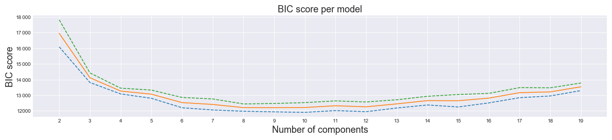
Figure 1BIC score versus the specified number of classes K for UKESM1 data. The solid line is the mean BIC value, and the dashed lines represent 1 standard deviation on either side of the mean.
3.1 Classification of ozone profiles from different experiments
In this section, we analyze the general vertical structure of ozone data from the UKESM simulations that represent a chosen historical period (2009–2014) and two future projection datasets, as mentioned in Sect. 2.1. Our results are not especially sensitive to the choice of any particular dataset from the three experiments since we train the GMM using all the profiles from each period from a variety of atmospheric ozone states. The classes are sorted by mean latitude for ease of interpretation.
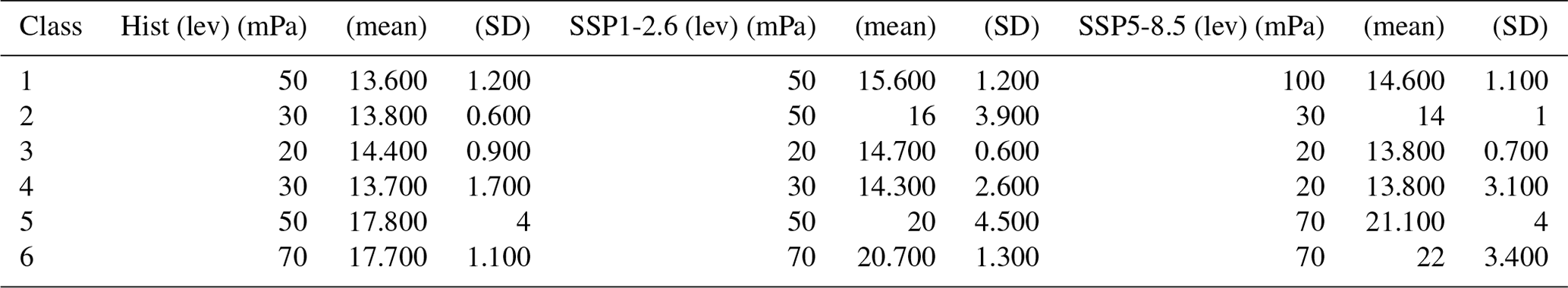
Proceeding from south to north: classes 1 and 2 are high-latitude Southern Ocean classes with similar mean profiles but different variability structures as measured by the standard deviation curves (Fig. 2). They both feature relatively low-altitude and gentle tropopauses, as indicated by the slope of the ozone curves. Class 1 has the lowest ozone value at 850 hPa (Table 1); it has a significant amount of variability in the middle stratosphere, which is associated with the ozone hole (Wargan et al., 2020), which has the largest effect on class 1, based on its intensification with respect to the season at high southern latitudes. The mean posterior probability, which in the context of a given statistical model is a measure of the algorithm's confidence in its assignment, is somewhat lower for class 2 than for class 1, indicating that there is some ambiguity associated with the assignments into class 2, which may be somewhat of a boundary or transition class between the high southern latitudes and the tropics. Note that high posterior probabilities do not necessarily indicate that the particular GMM is the best fit to the data, only that the selected GMM is confident in its assignment as measured by the uncertainty. Class 2 is also highly variable throughout the upper troposphere and tropopause but not as much as class 1. Notably, all of the high-latitude Southern Hemispheric classes feature relatively low lower-tropospheric ozone values with small variability – they are relatively “clean” in terms of surface ozone pollution (Table 1).
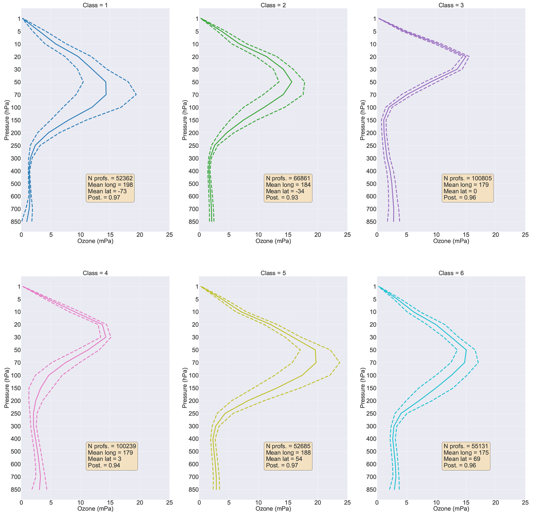
Figure 2Ozone concentration statistics of UK Earth System model data for the whole dataset, separated by class, as a function of pressure, sorted by latitude. Shown are the mean (solid lines) and the mean plus or minus 1 standard deviation (dashed line) for all profiles in the indicated class. Also shown are the number of profiles in each class and the class mean values for longitude, latitude, and posterior probability.
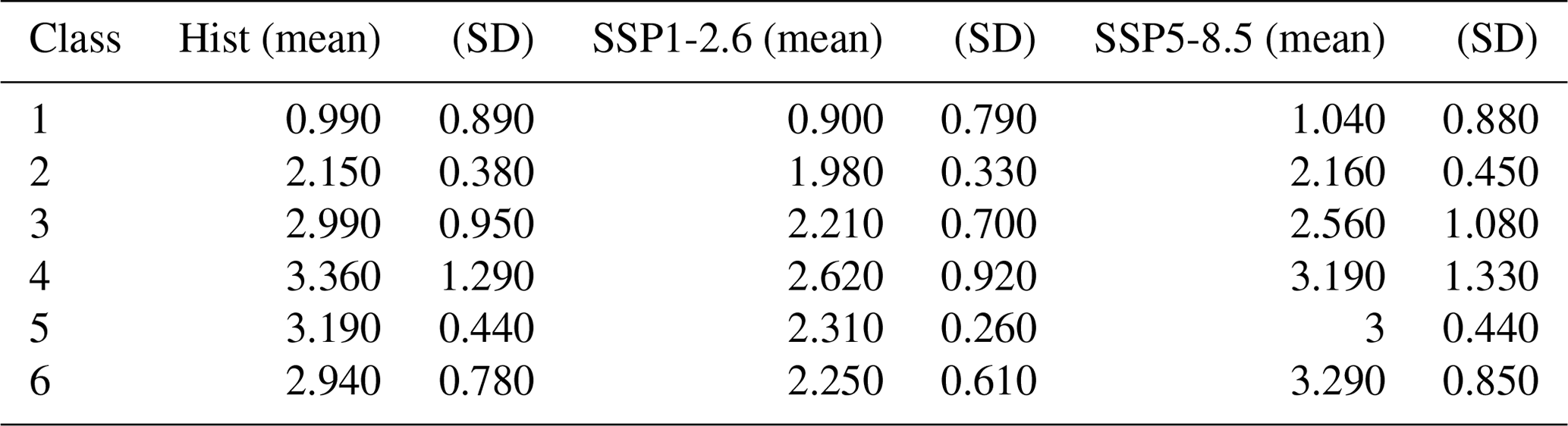
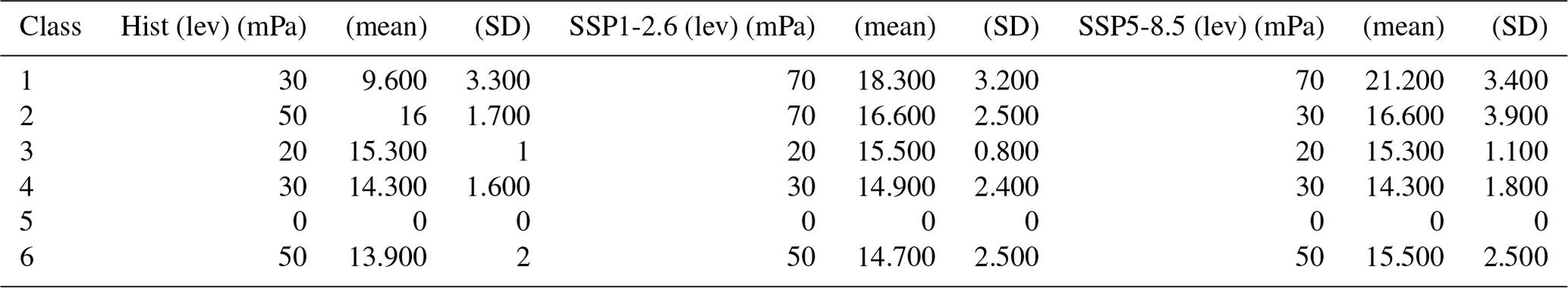
Table 1Ozone concentration statistics at 850 hPa for the historical, SSP126, and SSP585 experiments (shown in mPa) (from Fig. 2 but for each experiment).
Classes 3 and 4 are tropical classes, with higher lower-tropospheric ozone concentrations and a higher-altitude tropopause compared with the Southern Hemispheric classes (Fig. 2). Class 3 and class 4 share similar kinds of structures from the lower troposphere to the upper stratosphere. Class 4 features higher lower-tropospheric ozone and higher variability than class 3. Finally, classes 5 and 6 are Northern Hemispheric classes with high lower-tropospheric ozone concentrations and large variability from the tropopause to the stratosphere. The higher lower-tropospheric values result from greater surface pollutants in classes 4, 5, and 6, including the associated ozone precursor emissions, which tend to be concentrated in the Northern Hemisphere due to anthropogenic emissions (Monks et al., 2009, 2015).
Progressing from south to north, we see that the altitude of the maximum ozone concentration generally increases in height from the high-latitude Southern Hemisphere to the tropics and then decreases in height from the tropics to the high-latitude Northern Hemisphere (Fig. 2). This structure is consistent with observations and is enforced by the meridional Brewer–Dobson circulation (Butchart, 2014), which is associated with upwelling in the tropics and downwelling in the extratropics, somewhat favoring the Southern Hemisphere (Butchart, 2014; Li and Thompson, 2013; Newman and Todara, 2003; Weber et al., 2011). The imprint of this circulation pattern is a low-altitude tropopause at the poles and a higher-altitude tropopause at the Equator.
3.1.1 Classification of ozone profiles from historical experiment
The vertical ozone structure change pattern is complex following seasonal variation. To examine how the spatial pattern of the classes changes with seasons, global mean ozone concentrations are plotted according to seasonal categorization. The label map indicates the geographic distribution of the classes during 2009–2014 (Fig. 3). Notably, although the GMM algorithm was not given any latitude or longitude information, it was nevertheless able to identify spatially coherent groups. The tropical classes are largely organized into roughly zonal bands in each season, with some exceptions (e.g., June–August), where the Southern Hemispheric and tropical classes shift to the northernmost position (Fig. 3c).
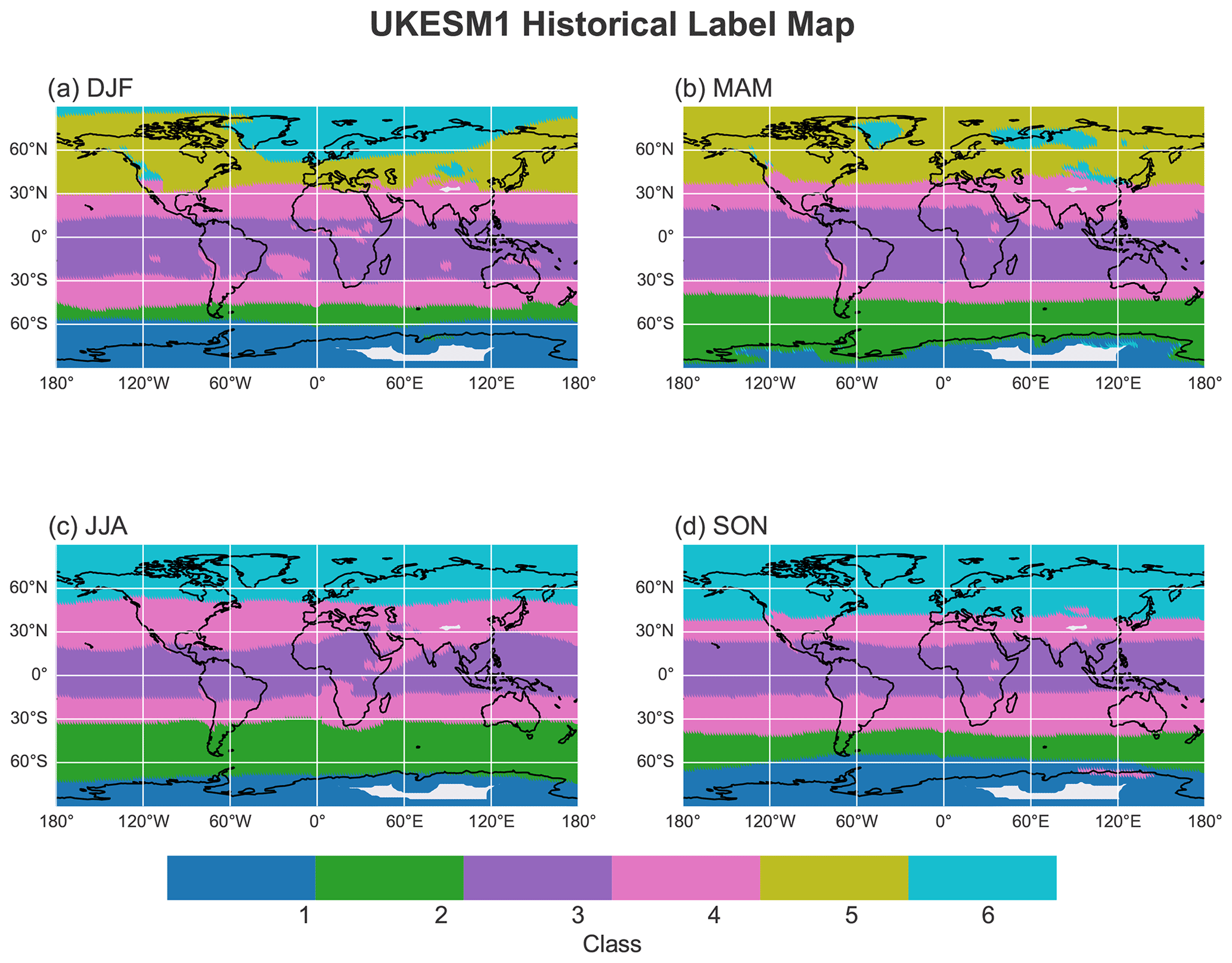
Figure 3Map of profiles color coded with the class they have been attributed to for model historical data (seasonal mean profiles covering 2009–2014 at each model grid cell) at 850 hPa.
Figure 2 shows that, from the tropopause to the stratosphere, the high-latitude and polar classes feature a relatively large standard deviation, especially in the lower and middle stratosphere, suggesting that these classes consist of a wide variety of profiles. These high-latitude classes are more sensitive to seasonal change than tropical classes. For example, from Fig. 3, class 1 (with the largest standard deviation at stratosphere) extends up to 40∘ S during December–February (DJF), recedes southward during March–May (MAM), and starts migrating northward again during June–August (JJA). It reaches its northernmost position again in September–November (SON). The stratospheric ozone (14.33 ± 5.07 mPa) suggests that, depending on the strength Antarctic ozone hole, this value varies with the season, and during SON the region covered by class 1 contains the lowest amount of stratospheric ozone (Table D4). On the other hand, class 2 starts shifting northward during MAM and reaches its northernmost position during JJA. Since the southern polar vortex is much stronger, it prevents the mixing of classes 1 and 2 during the southern fall and winter seasons. The tropical classes are less variable, except for DJF and JJA. The tropical classes shift to the southernmost position during the former and expand up to around 50∘ N during the latter. Class 3 expands most northward during MAM. The widening trends based on seasonality imply that the tropical broadening in the Southern Hemisphere is mainly due to the Antarctic ozone hole, which causes the largest radiative cooling effect in the lower stratosphere during DJF (Palmeiro et al., 2014). Increasing black carbon and tropospheric ozone are considered major forcings for Northern Hemisphere tropical class widening on a longer timescale during JJA (Allen et al., 2012). However, these two forcings together have the largest warming effect in the Northern Hemisphere extratropics (Hu et al., 2018). Studies showed that the shallow branch (located in the lowermost stratosphere with upwelling in the tropics and downwelling in the subtropics) of tropical upwelling is much stronger toward the summer hemisphere during DJF than JJA (Palmeiro et al., 2014). The deep branch with upwelling in the upper stratosphere in the tropics and downwelling in the middle and high latitudes also show a similar seasonal cycle with downwelling extended to the polar latitudes in the stratosphere (Seviour et al., 2012; Palmeiro et al., 2014). The differentiation between the two branches is based on different forcing, planetary-scale wave forcing acts on the shallow branch, and in the deep branch the upwelling is associated with greenhouse gas increases (Palmeiro et al., 2014). However, the investigation of seasonal change in tropical upwelling in shallow and deep branches is beyond the scope of this study.
The northern high-latitude classes are characterized by frequent variability. Spatially, Class 5 is a dominant northern subpolar and polar class during DJF and MAM. For the remainder of the year, class 5, with a very high amount of stratospheric ozone concentration (Fig. 2), is absent, and class 6 dominates the entire region (Fig. 3c and d). This tendency suggests to us that Arctic high-altitude ozone is stronger during Northern Hemispheric winter and spring and weaker for the rest of the year (Appendix D).
The high lower-tropospheric ozone concentration in classes 4 and 5 (Table 1) highlights anthropogenic emissions over those regions and the bulk of biomass burning and wildfire, which occurs primarily near the Arctic Circle, in Africa, and in some parts of North America (Laban et al., 2018; Jaffe and Wigder, 2012). In the last few decades, wildfires and biomass burning have gained much attention as they have been recognized as the second-largest source of ozone precursor emissions (Monks et al., 2015). Boreal forest fires are a known source of high surface ozone over North America (Jaffe and Wigder, 2012). Biomass burning in Africa produces a significant amount of ozone precursor. Arctic boreal fire and biomass burning are sources of high ozone precursors over the northern extratropical and temperate zone (Laban et al., 2018; Monks et al., 2015; Jaffe and Wigder, 2012).
Classes at the northern high latitudes (i.e., class 5) have more stratospheric ozone than those at southern high latitudes (i.e., classes 1 and 2), and this class peaks during DJF and MAM (Tables D1 and D2). This indicates that in our study the Northern Hemisphere ozone hole is not especially predominant during these months in the seasonal mean. However, Dunn et al. (2022) showed that there are some particular years when the polar ozone hole can happen in Northern Hemisphere spring. Larger amplitudes of upward-propagating planetary waves like Rossby waves can propagate from troposphere to stratosphere with eastward wind, where these waves can perturb stratospheric circulation and reduce the speed of polar night jet (Lee, 2021; Oehrlein et al., 2020; Waugh et al., 2017). In the Northern Hemisphere, the continent and mountain range layouts accelerate this wave activity more than in the Southern Hemisphere (Lee, 2021; Waugh et al., 2017). Consequently, the Arctic stratospheric vortex is much weaker and more variable than its Antarctic counterpart, which features larger meanders in the meridional extent. It is for this reason that, unlike the Antarctic, a large ozone hole does not form in the Arctic stratosphere each winter. As the Arctic temperature is higher than the Antarctic, a strong Antarctic vortex allows for the formation of polar stratospheric clouds that catalyze ozone depletion (Waugh et al., 2017; Lee, 2021; Newman and Todara, 2003). This allows redistribution of stratospheric ozone and pulls ozone from the tropics in the Northern Hemisphere (Lee, 2021; Newman and Todara, 2003). The strong polar vortex at the South Pole prevents the region from having high stratospheric ozone (Newman and Todara, 2003), especially during the Antarctic spring season.
3.2 Classification of ozone profiles in the future climate projections SSP1-2.6 and SSP5-8.5
We examine the distribution and structure of ozone in two chosen future climate projections, namely SSP1-2.6 and SSP5-8.5. SSP1-2.6 is a scenario with strong emission reductions, and SSP5-8.5 is a scenario with increased emissions. We chose these two experiments as end-members representing two drastically different future projections. In the SSP1-2.6 case, with reduced emissions of ozone precursors, the total lower-tropospheric ozone concentration gets smaller (Table 1). In the SSP5-8.5 case, with increased emissions of ozone precursors, the total lower-tropospheric ozone concentration is slightly increased or approximately steady (Table 1).
Classes 1 and 6, in particular, which are affected by the ozone hole because of their geographical location, display a variation in stratospheric ozone (Appendix D) between 2009–2014 and 2095–2100 in both cases in each season, but SON dominates the increase in stratospheric ozone for the Southern Hemisphere (Table D4), which is a signature of the closing of the ozone hole (Keeble et al., 2021). The maximum concentration is located around 30 hPa in the historical case, which is above the region of maximum ozone depletion. The recovery of the ozone hole also shifts the level of maximum ozone concentration to lower altitudes (higher pressures, i.e., from 30 to 70 hPa) for the Southern Hemisphere in future projections of the austral spring season (Table D4). In the following subsections, we investigate differences in the spatial structure of the two future emissions experiments.
3.2.1 Geographical distribution of ozone profiles in SSP1-2.6
Here we examine the spatial pattern of ozone profiles in SSP1-2.6 in each season over the period 2095–2100. As with the historical experiment, class 1 has the lowest 850 hPa ozone (Table 1), which is consistent with the reduction in surface ozone precursors in this experiment. The maximum value of stratospheric ozone increases under this scenario, which is a signature of the recovery of the ozone hole (Keeble et al., 2021).
Moving northwards, class 2 appears to have a similar structure to its historical counterpart, with higher stratospheric ozone and considerable variability in the upper troposphere to the middle atmosphere (Fig. 2). It is a midlatitude Southern Hemispheric class occupying roughly the same total surface area as it did in the historical experiment (Figs. 3 and 4). Unlike the historical case, the area occupied by class 3 has decreased during DJF, and in other seasons this class also shifts northward and southward as in the historical case (Fig. 4). This suggests strong emissions play a vital role for class 3. Notably, the relative position of class 2 sits next to class 6 during DJF and SON, indicating that these two classes may be difficult to unambiguously differentiate over these seasons because of their similar structure. The geographic distributions of classes 5 and 6 are similar to their historical counterpart, except with reduced lower-tropospheric ozone concentrations consistent with continued ozone precursor emissions reductions (Table 1) and increased stratospheric ozone during DJF and MAM (Tables D1 and D2). The tropospheric ozone decrease is more significant in the Northern Hemisphere than in other scenarios, helping to mitigate climate change and air quality impacts (Table 1) (Keeble et al., 2021).
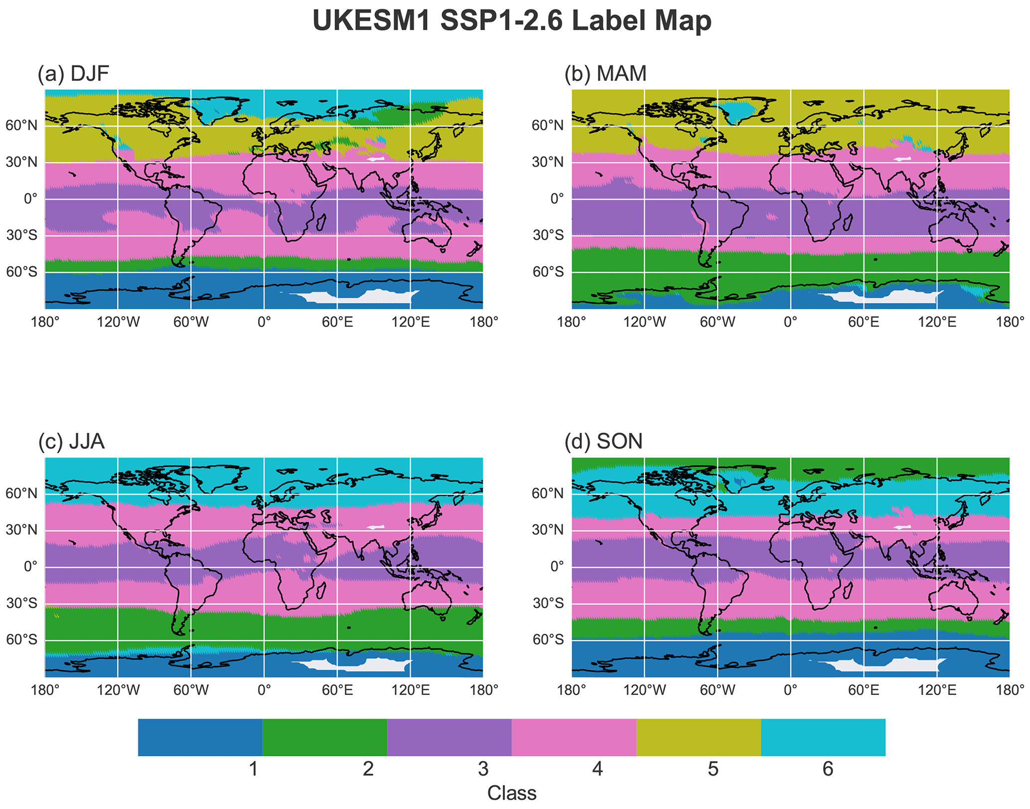
Figure 4The same as Fig. 3 but for the SSP 1.2-6 label map covering the years 2095–2100.
3.2.2 Geographical distribution of ozone profiles in SSP5-8.5
Here, we examine the structure of atmospheric ozone in the 2095–2100 period of the SSP5-8.5 experiment. In this experiment, ozone mixing ratios are generally higher throughout much of the troposphere and upper stratosphere. In the troposphere, the drivers of this increase are complex. Under the assumptions of the SSP5-8.5 scenario, global mean emissions of nitrogen oxides (NOx) and carbon monoxide (CO) are lower in 2095 than in the present day, while global mean emissions of methane (CH4) are higher (Gidden et al., 2019). However, changes in ozone precursor emissions (including biogenic volatile organic compound (BVOC) emissions caused by increasing tropospheric temperature) alone do not drive tropospheric ozone changes. The availability of tropospheric water vapor and stratosphere-to-troposphere transport of ozone together drive increases in tropospheric ozone concentrations (Griffiths et al., 2021; Turnock et al., 2020; Zanis et al., 2022). In the stratosphere, this increase is simpler to understand. Upper-stratospheric ozone increases under all SSPs as ozone-depleting substances decrease but increases more in scenarios that assume larger increases in greenhouse gas emissions due to the resulting CO2-induced cooling of the stratosphere and the impacts this has on gas-phase chemistry (Haigh and Pyle, 1982; Jonsson et al., 2004).
Proceeding from south to north, we see that classes 1 and 2 are similar to their historical counterparts during DJF and MAM, covering a similar proportion of area, albeit with increased stratospheric ozone at the pressure level with maximum concentration during JJA and SON that decreases during both DJF and MAM unlike SSP 1-2.6 and the historical case (Appendix D). Future ozone depletion decrease will lead to ozone concentration increases throughout the atmosphere, and the high-latitude upper stratosphere of both hemispheres will have the largest changes (Griffiths et al., 2021). However, an increasing amount of greenhouse gas emission will yield a more complex pattern of ozone changes, which will lead to a possible strengthening of the Brewer–Dobson circulation and an increase in net stratospheric influx and high tropospheric ozone in the Southern Hemisphere class as the result of circulation changes (Young et al., 2013; Monks et al., 2015; Butchart, 2014; Griffiths et al., 2021; Lu et al., 2019).
The tropical classes (i.e., 3 and 4) are similar to those seen in the historical case, except for JJA. During JJA, class 3 is more sparse in the Southern Hemisphere. Interestingly class 5 starts showing up in the southern polar region during JJA (Fig. 5). This experiment is associated with an enhanced amount of ozone mixing ratio, which causes the polar vortex to weaken. As a result, during Southern Hemisphere winter, a huge amount of stratospheric ozone sits next to class 1. Finally, class 6 remains a large-scale Northern Hemispheric polar class during JJA and SON, although class 6 has increased lower-tropospheric ozone concentrations relative to SSP1-2.6, in part due to continued precursor emissions. In response to tropospheric warming driven by greenhouse gas in SSP5-8.5, the subtropical tropospheric jets intensify, while the contribution of gravity waves increases in the middle stratosphere (Palmeiro et al., 2014). As a result, stratospheric ozone increases in high-latitude classes (Table D).
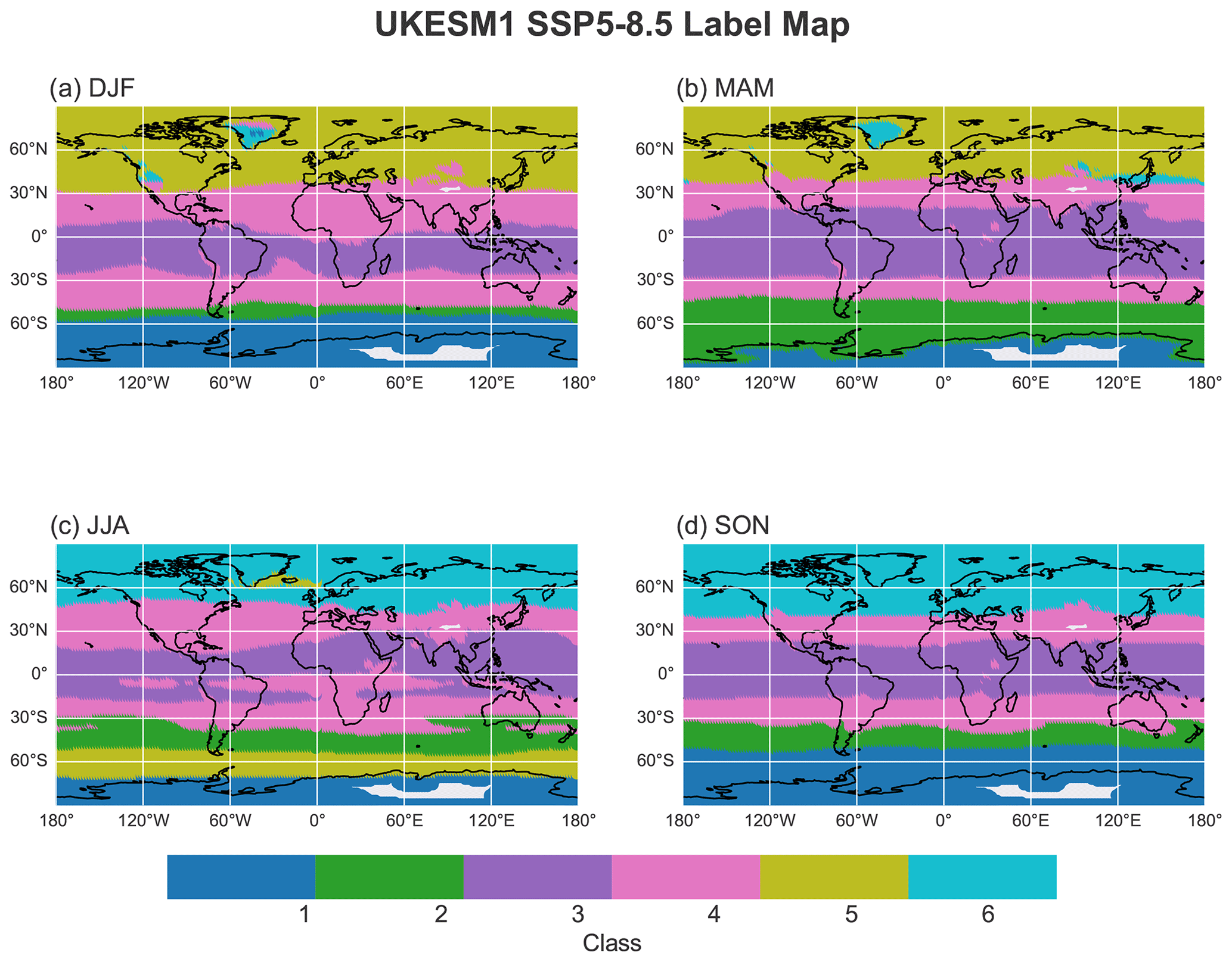
Figure 5The same as Fig. 3 but for the SSP5.8-5 label map covering the years 2095–2100.
The oceans are major sinks of tropospheric ozone at the surface, and there are few direct sources of ozone precursors present over the ocean (Archibald et al., 2020a, b). Advection of emission-driven ozone production over the land or an increase in ozone transport from the stratosphere is responsible for ozone increase for the profiles that are covering the ocean (e.g., class 3, which covers the majority of the oceanic region in the tropics) (Archibald et al., 2020a, b).
The distribution of ozone in the atmosphere is relevant for both climate and human health. Recently, researchers have employed a number of approaches for identifying different “profile types” in both observational and numerical model data, going beyond a basic latitudinal-averaging framework for comparison. These methods complement each other and add to existing expertise-driven classification approaches. Here we aimed to add to the atmospheric analysis toolbox using unsupervised classification, which is a type of machine learning that identifies patterns and structures in unlabeled datasets. We based our profile classification scheme on Gaussian mixture modeling (GMM), which attempts to represent the ozone profiles as represented in an abstract principal component space using a linear combination of Gaussian functions. We applied GMM to a collection of seasonal mean ozone profiles taken from a set of UKESM1 simulations. Specifically, we used GMM to classify profiles from a historical experiment and two future climate experiments, namely SSP1-2.6 and SSP5-8.5. We used GMM as a “hypothesis generation tool”, generating ideas for further exploration and analysis (Kaiser et al., 2022). Note that the detailed exploration of this hypothesis is beyond the scope of this technical note; further analysis of the ideas presented here would be a welcome addition to the literature. The spatial extent and seasonal variability within the classes reflect the integrated effect of a number of different processes and timescales, so they should be interpreted within that context. Nevertheless, GMM was indeed able to identify spatially coherent profile types and track their variability over time, highlighting the ability of GMM to identify and follow structures.
Even though the GMM algorithm was not supplied with the latitudes or longitudes of the profiles, the classes nevertheless vary structurally with latitude, as expected. For example, we find two tropical classes (classes 3 and 4) with elevated tropopause heights and two polar classes (classes 1 and 6) with lower tropopause heights, broadly consistent with the imprint of the Brewer–Dobson circulation.
The spatial distributions of the classes generally vary with the season. In the historical UKESM1 experiment, we see that the tropical classes (classes 3 and 4) shift in mean latitude towards the summer pole, i.e., southwards in DJF and northwards in JJA. The subpolar and polar classes in the Northern Hemisphere (classes 5 and 6) vary drastically, with class 5 disappearing entirely in summer and autumn. This may reflect larger variability in the profile structure seen in autumn and winter. In the Southern Hemisphere, the southernmost class (class 1) usually covers Antarctica, except in the autumn and winter (MAM, JJA) when class 2 covers a larger area. We see similar patterns in SSP1-2.6 and SSP5-8.5, with the notable exception of the appearance of class 5, ostensibly a Northern Hemispheric class, in the wintertime Southern Hemisphere of SSP5-8.5. This result highlights that the classes are not inextricably tied to a particular latitude band: they may appear wherever similar structures exist. The appearance of class 5 here suggests a shift in ozone distribution large enough that it disrupts the classification scheme, highlighting an area for further study.
Our results for SSP1-2.6 are broadly consistent with the tropical broadening hypothesis in that the spatial extent of the tropical classes (classes 3 and 4) increases between the historical case and SSP1-2.6 across all seasons. We also saw increases under SSP5-8.5, with the possible exception of SON. In the projections of future climate considered here, both hemispheric high latitudes show large variations in stratospheric ozone. These changes in the ozone concentration for high-latitude classes (i.e., classes 1 and 6) in future projections show the potential changes due to changes in precursor emissions and changes in ozone advection. Southern Hemispheric tropospheric ozone levels are generally low for all three cases considered here. There are larger fluctuations in the lower troposphere at high latitudes of the Northern Hemisphere (class 6), which could be related to differences in precursor transport and chemistry from lower latitudes.
This study focuses on model analysis. When working with model data, we typically have access to fairly uniform spatial and temporal ozone coverage, at least in parts of the atmosphere with a full range of pressures from 850 to 1 hPa. This coverage allows us to train our mixture model in a way that is relatively unbiased with respect to location and time. The trained mixture model is thus able to identify coherent regimes with similar patterns of vertical variability in a way that is more general than drawing somewhat arbitrary latitude–longitude boxes. Because we can train the mixture model using data from a variety of times and experiments, it is possible to train a GMM that can, in principle, represent the full range of data structures found within a selected ensemble and track how those structures evolve over time. Although we did not attempt to do so here, it should be possible to use GMM for inter-model comparison, allowing for the structures and differences in structures to be derived directly from model data.
Although our study focused on model analysis, it is possible to apply GMM to observed ozone profiles as well. At present, ozone observations are biased towards a few specific locations where long-term monitoring has taken place. Training a GMM on this data would necessarily bias the classes towards particular locations and times, making direct comparisons between models and observations difficult. One possible solution would be to train a GMM on model data and then apply it to observations, although any systematic biases would have to be treated carefully during the data cleaning and prepossessing steps. In terms of working towards a more optimized ozone observing system, it may be useful to use GMM and similar classification methods to identify which regions feature coherent variability.
Table 2Relative area coverage by tropical classes (3+4) as combined regions during each season (shown as percentages).
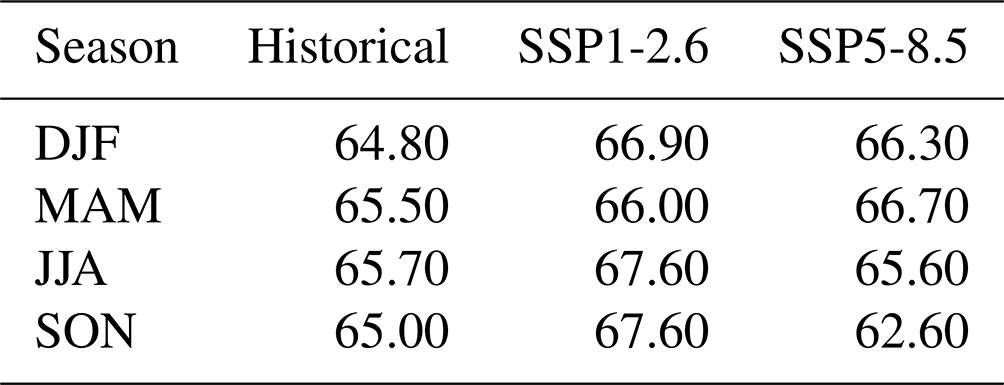
In this study, we applied Gaussian mixture modeling (GMM), an unsupervised classification method, to ozone profiles from the UKESM1 coupled climate model in order to robustly and objectively identify coherent sets of ozone profile types. Our motive was to investigate the ozone structure using a limited number of classes. We used principal component analysis (PCA) to reduce the computational complexity of the problem, increasing the computational efficiency at the expense of only 1 % of the variability in the dataset. We used a statistical approach (i.e., BIC) and post hoc expert judgment to inform our choice of the number of classes, settling on a six-class representation of the ozone profiles. This six-class system included two tropical classes and four mid-latitude to high-latitude classes. Although the GMM algorithm was not given any spatiotemporal information, we found that it was able to identify a set of spatially coherent regions of ozone structure. We trained the GMM using data from all three model cases in order to expose it to the full range of profile types in our classification problem. We compared lower troposphere and maximum ozone concentrations for three model cases and their spatial extents. Higher concentrations of stratospheric ozone in classes 1 and 6 in both of the future projection cases indicate a seasonal decrease in ozone depletion and possible ozone hole recovery, which results in a decrease in tropopause height based on seasons (Appendix D). The modeled lower-tropospheric ozone is higher in the Northern Hemisphere and relatively low in the Southern Hemisphere (Table 1). Notably, the spatial area occupied by the tropical classes increased in both future projections based on seasonality relative to the historical benchmark, consistent with the tropical broadening hypothesis, i.e., the expected expansion of tropical upwelling (Table 2). GMM can be applied to identify data-derived regions of coherent ozone structure and may therefore be useful for model–model comparisons or model–data comparisons.
The principal component analysis shown in Fig. A1 is adopted for dimensionality reduction in this work. The figure shows the eigenfunctions. These eigenfunctions came from the eigenvalues, and the corresponding eigenvectors of the covariance matrix are used to find the directions along which the variability is the largest.

Figure A1Principal components (PCs) showing the percent variance statistically explained by each PC (in parentheses).
For details of the GMM classification algorithm, we refer the readers to Bishop (2006). The classification algorithm is adopted from Bishop (2006) and Maze et al. (2017).
B1 Probability density function of profiles
The key ingredient of GMM is a multidimensional normal probability density function (PDF) with mean μ and covariance Σ:
In this study, is a profile of the collection, μk is a D-dimensional mean vector where , is a covariance matrix, and is the determinant.
In other words, the array X is the dataset we want to analyze; it is made up of N vertical profiles (as columns) of D pressure levels (as rows). The functional dependence of the Gaussian on the x is through the quadratic form, , which appears in the exponent in Eq. (B1). We consider a superposition of K Gaussian densities of the form, where the quantity Δ is called the “Mahalanobis distance” from μ to x, which reduces to the Euclidean distance when Σ is the identity matrix (Bishop, 2006).
The joint distribution will be p(z)p(x|z), and the marginal distribution of x is
Here, is the probability distribution for the observations . Thus, for every observed data point xn, there is a corresponding latent variable zn.
GMM represents the PDF as a weighted sum of K Gaussian classes as in Eq. (1). If we integrate Eq. (B1) with respect to x and note that both p(x) and Gaussian components are normalized, we obtain
We call the parameters λk mixing coefficients. The requirement p(x)≥0 together with implies λk≥0 for all k.
Combining these conditions, we can write . The latent variable z is a K-dimensional binary random variable, having a 1-of-K representation in which a particular element zk=1 and the rest are equal to 0. Therefore, and , and there are K possible states for the vector z according to which element is nonzero. The joint distribution is p(x,z) in terms of a marginal distribution p(z) and a conditional distribution p(x|z). The marginal distribution over z is specified in terms of the mixing coefficients λk, such that
Because z uses a 1-of-K representation, Eq. (1) can be written in the following form:
The conditional distribution of x given a particular value for z is a Gaussian
which can be written in the following form:
The joint distribution will be p(z)p(x|z), and the marginal distribution of x is
This equation is also called “mixture distribution”.
Here, p(x) stands for the observed PDF, and is the probability distribution for the observations . Thus, for every observed data point xn, there is a corresponding latent variable zn.
Gaussian mixture modeling boils down to an optimization problem that can be tackled by maximizing the likelihood of observed profiles. This optimization is referred to as a “model training”. It is solved with the expectation–maximization (EM) method. The conditional probability of z given x plays an important role in the EM algorithm. γ(zk) represents , whose value can be found using Bayes' theorem,
Therefore,
Here, λk is the prior probability of zk=1 and the quantity γ(zk) as the corresponding posterior probability once we have observed x. The posterior probability for each component in GMM from which the dataset was generated is called the “responsibility”. Responsibilities sum to 1. This helps us predict which Gaussian is responsible for which data point.
Since the latent variables are never observed, and the correct values are not known in advance, EM is useful to figure out what z represents without someone to specify it beforehand.
The EM method aims to iteratively improve the results based on some initial assumptions regarding the mean, standard deviation, and latent values. Every single iteration consists of the following two steps: the expectation (E) step and the maximization (M) step.
In the E step, it uses current values for the parameters to evaluate the posterior probabilities or responsibilities given by Eq. (B8). We then use these probabilities in the M step to re-estimate the means, covariances, and mixing coefficients.
EM for Gaussian mixtures
-
Initialize the parameters and evaluate the initial values for log-likelihood. Parameters are as follows: means μk, covariances Σk, and mixing coefficients λk.
-
In the E step, evaluate the responsibilities using the current parameter values:
-
In the M step, re-estimate the parameters using the current responsibilities:
-
,
-
,
-
,
where .
-
-
Evaluate the log likelihood using the following equation:
and check the result for convergence of either the parameters or the log-likelihood. If the convergence criterion is not satisfied, return to step 2.
The main free-input parameter to the model training procedure is the number of mixture components K. Determining the most appropriate number of components automatically is a difficult problem that often contains a degree of subjectivity, requiring domain expertise. Here we use a combination of statistical guidance and expert judgment to select the number of classes.
For statistical guidance, we use the Bayesian information criterion (BIC). The BIC is an empirical approach to model probability computed as follows:
where ℓ(K) is the log-likelihood of the trained model with K classes and n is the number of profiles used in the BIC test. The log-likelihood function is as follows:
The log-likelihood of the dataset, assuming independent observations, is as follows:
where it is explicit that the log-likelihood is a function of the set of parameters θ and that p(xi;θ) is the probability given in Eq. (C2) for the dataset instance xi using the parameter θ. Nf is the sum of the component weights to be estimated, Gaussian means, and covariance matrix elements in the D-dimensional data space (where our new dimension is d after PCA):
The BIC is empirical; the first term on the right-hand side in Eq. (C1) decreases as the likelihood of the statistical model increases, while the second term on the right-hand side is a penalty term that increases with K and thus discourages overfitting (Maze et al., 2017). The “ideal” value for K, in terms of this statistical metric, would be one that minimizes BIC, i.e., where the likelihood of the model has been maximized without overfitting. One may also find that the BIC curve “plateaus”, indicating that the model has reached maximum likelihood; i.e., further increases in the statistical complexity of the model no longer noticeably improve the likelihood. Empirical approaches like BIC are often used in statistics, especially when constraining the parameters is difficult or subjective. They can give us a rough estimate of what data collection might look like if we were able to survey the entire population (Maze et al., 2017).
Here, is the set of parameters that minimize the misfit between the PDF of the dataset that is going to be used for calculation and the PDF of the original dataset. To train a GMM, i.e., to maximize ℓ(θ) with regard to θ so that our BIC can be lowest, we need a dataset x and a given number of components K (Maze et al., 2017).
Here we provide detailed information about the maximum ozone concentration based on seasons.
Table D1Pressure level (lev) of the maximum value of class mean ozone concentration during DJF. The mean and standard deviation values of the class statistics are also shown (in mPa).


Data from UKESM1 are part of the CMIP6 data suite, which is freely available from a number of sources. For this study, we used the Pangeo platform (https://pangeo.io/, last access: 22 November 2022) for rapid data access and averaging. The DOIs used are as follows: https://doi.org/10.22033/ESGF/CMIP6.6113, Tang et al., 2019; https://doi.org/10.22033/ESGF/CMIP6.6333, Good et al., 2019a; https://doi.org/10.22033/ESGF/CMIP6.6405, Good et al., 2019b. We used a “preprocessing” script from Julian Busecke (https://github.com/jbusecke/cmip6_preprocessing, last access: 21 January 2023; DOI: https://doi.org/10.5281/zenodo.7519179, Busecke et al., 2023). All scripts used to process the data and produce the figures for this paper are available online via Zenodo (https://doi.org/10.5281/zenodo.7662179, Fahrin and Jones, 2023).
DCJ designed the initial project and developed much of the software. FF performed the analysis, worked with the software, and created the figures. JK and ATA provided expert guidance on analyzing the results and placing them in the wider context of atmospheric chemistry. FF and DCJ wrote the initial manuscript, JK edited the introduction, and all authors assisted with edits.
The contact author has declared that none of the authors has any competing interests.
Publisher's note: Copernicus Publications remains neutral with regard to jurisdictional claims in published maps and institutional affiliations.
This work originated as a master's project in the Department of Mathematical Sciences at Georgia Southern University. The authors wish to thank Guillaume Maze for suggesting the particular training dataset method used here. We acknowledge the use of the Pangeo platform in obtaining our data (https://pangeo.io/, last access: 22 November 2022). Daniel C. Jones acknowledges funding from a UKRI Future Leaders Fellowship (grant no. MR/T020822/1) and the North Atlantic Climate System Integrated Study (ACSIS) (grant no. NE/N018028/1). James Keeble and Alexander T. Archibald thank the Met Office CSSP-China programme for funding the POzSUM project. The authors thank two anonymous reviewers for their helpful comments on the manuscript.
This research has been supported by the Natural Environment Research Council, British Antarctic Survey (grant no. NE/N018028/1), and the UK Research and Innovation, Natural Environment Research Council (grant no. MR/T020822/1).
The article processing charges for this open-access publication were covered by the Iowa State University Library.
This paper was edited by Jianzhong Ma and reviewed by two anonymous referees.
Abernathey, R. P., Augspurger, T., Banihirwe, A., Blackmon-Luca, C. C., Crone, T. J., Gentemann, C. L., Hamman, J. J., Henderson, N., Lepore, C., McCaie, T. A., Robinson, N. H., and Signell, R. P.: Cloud-Native Repositories for Big Scientific Data, Comput. Sci. Eng., 23, 26–35, https://doi.org/10.1109/MCSE.2021.3059437, 2021. a
Allen, R. J., Sherwood, S. C., Norris, J. R., and Zender, C. S.: Recent Northern Hemisphere tropical expansion primarily driven by black carbon and tropospheric ozone, Nature, 485, 350–354, 2012. a
Archibald, A., Neu, J., Elshorbany, Y., Cooper, O., Young, P., Akiyoshi, H., Cox, R., Coyle, M., Derwent, R., Deushi, M., Finco, A., Frost, G. J., Galbally, I. E., Gerosa, G., Granier, C., Griffiths, P. T., Hossaini, R., Hu, L., Jöckel, P., Josse, B., Lin, M. Y., Mertens, M., Morgenstern, O., Naja, M., Naik, V., Oltmans, S., Plummer, D. A., Revell, L. E., Saiz-Lopez, A., Saxena, P., Shin, Y. M., Shahid, I., Shallcross, D., Tilmes, S., Trickl, T., Wallington, T. J., Wang, T., Worden, H. M., and Zeng, G.: Tropospheric Ozone Assessment ReportA critical review of changes in the tropospheric ozone burden and budget from 1850 to 2100, Elementa: Science of the Anthropocene, 8, 2325–1026, https://doi.org/10.1525/elementa.2020.034, 2020a. a, b
Archibald, A. T., Turnock, S. T., Griffiths, P. T., Cox, T., Derwent, R. G., Knote, C., and Shin, M.: On the changes in surface ozone over the twenty-first century: sensitivity to changes in surface temperature and chemical mechanisms, Philos. T. Roy. Soc. A, 378, 20190329, https://doi.org/10.1098/rsta.2019.0329, 2020b. a, b
Banerjee, A., Maycock, A. C., Archibald, A. T., Abraham, N. L., Telford, P., Braesicke, P., and Pyle, J. A.: Drivers of changes in stratospheric and tropospheric ozone between year 2000 and 2100, Atmos. Chem. Phys., 16, 2727–2746, https://doi.org/10.5194/acp-16-2727-2016, 2016. a
Bates, D. R. and Nicolet, M.: The photochemistry of atmospheric water vapor, J. Geophys. Res., 55, 301–327, 1950. a
Bishop, C. M.: Pattern recognition, Mach. Learn., 128, https://link.springer.com/book/9780387310732 (last access: 20 June 2022), 2006. a, b, c, d, e
Boehme, L. and Rosso, I.: Classifying Oceanographic Structures in the Amundsen Sea, Antarctica, Geophys. Res. Lett., 48, e2020GL089412, https://doi.org/10.1029/2020GL089412, 2021. a
Boleti, E., Hueglin, C., Grange, S. K., Prévôt, A. S. H., and Takahama, S.: Temporal and spatial analysis of ozone concentrations in Europe based on timescale decomposition and a multi-clustering approach, Atmos. Chem. Phys., 20, 9051–9066, https://doi.org/10.5194/acp-20-9051-2020, 2020. a
Busecke, J., Ritschel, M., Maroon, E., Nicholas, T., and readthedocs-assistant: jbusecke/xMIP: v0.7.1, Zenodo [data set], https://doi.org/10.5281/zenodo.7519179, 2023. a
Butchart, N.: The Brewer-Dobson circulation, Rev. Geophys., 52, 157–184, 2014. a, b, c
Chameides, W. L., Fehsenfeld, F., Rodgers, M. O., Cardelino, C., Martinez, J., Parrish, D., Lonneman, W., Lawson, D. R., Rasmussen, R. A., Zimmerman, P., Greenberg, J., Mlddleton, P., and Wang, T.: Ozone precursor relationships in the ambient atmosphere, J. Geophys. Res.-Atmos., 97, 6037–6055, 1992. a
Chapman, S.: XXXV. On ozone and atomic oxygen in the upper atmosphere, The London, Edinburgh, and Dublin Philosophical Magazine and Journal of Science, 10, 369–383, 1930. a
Cicerone, R. J., Stolarski, R. S., and Walters, S.: Stratospheric ozone destruction by man-made chlorofluoromethanes, Science, 185, 1165–1167, 1974. a
Crutzen, P. J.: The influence of nitrogen oxides on the atmospheric ozone content, Q. J. Roy. Meteor. Soc., 96, 320–325, 1970. a
Desbruyères, D., Chafik, L., and Maze, G.: A shift in the ocean circulation has warmed the subpolar North Atlantic Ocean since 2016, Communications Earth & Environment, 2, 48, https://doi.org/10.1038/s43247-021-00120-y, 2021. a
Diab, R., Thompson, A., Mari, K., Ramsay, L., and Coetzee, G.: Tropospheric ozone climatology over Irene, South Africa, from 1990 to 1994 and 1998 to 2002, J. Geophys. Res.-Atmos., 109, D20301, https://doi.org/10.1029/2004JD004793, 2004. a, b
Dunn, R. J., Aldred, F., Gobron, N., et al.: Global climate, B. Am. Meteorol. Soc., 103, S11–S142, 2022. a
Eyring, V., Arblaster, J. M., Cionni, I., Sedláček, J., Perlwitz, J., Young, P. J., Bekki, S., Bergmann, D., Cameron-Smith, P., Collins, W. J., Faluvegi, G., Gottschaldt, K.-D., Horowitz, L. W., Kinnison, D. E., Lamarque, J.-F., Marsh, D. R., Saint-Martin, D., Shindell, D. T., Sudo, K., Szopa, S., and Watanabe, S.: Long-term ozone changes and associated climate impacts in CMIP5 simulations, J. Geophys. Res.-Atmos., 118, 5029–5060, 2013. a
Fahrin, F. and Jones, D.: UKESM1_Ozone_clustering: UKESM1 Seasonal Ozone Profiles Clustering, Zenodo [code and data set], https://doi.org/10.5281/zenodo.7662179, 2023. a
Gidden, M. J., Riahi, K., Smith, S. J., Fujimori, S., Luderer, G., Kriegler, E., van Vuuren, D. P., van den Berg, M., Feng, L., Klein, D., Calvin, K., Doelman, J. C., Frank, S., Fricko, O., Harmsen, M., Hasegawa, T., Havlik, P., Hilaire, J., Hoesly, R., Horing, J., Popp, A., Stehfest, E., and Takahashi, K.: Global emissions pathways under different socioeconomic scenarios for use in CMIP6: a dataset of harmonized emissions trajectories through the end of the century, Geosci. Model Dev., 12, 1443–1475, https://doi.org/10.5194/gmd-12-1443-2019, 2019. a
Good, P., Sellar, A., Tang, Y., Rumbold, S., Ellis, R., Kelley, D., and Kuhlbrodt, T.: MOHC UKESM1.0-LL model output prepared for CMIP6 ScenarioMIP ssp126, Earth System Grid Federation [data set], https://doi.org/10.22033/ESGF/CMIP6.6333, 2019a. a
Good, P., Sellar, A., Tang, Y., Rumbold, S., Ellis, R., Kelley, D., and Kuhlbrodt, T.: MOHC UKESM1.0-LL model output prepared for CMIP6 ScenarioMIP ssp585, Earth System Grid Federation [data set], https://doi.org/10.22033/ESGF/CMIP6.6405, 2019b. a
Griffiths, P. T., Murray, L. T., Zeng, G., Shin, Y. M., Abraham, N. L., Archibald, A. T., Deushi, M., Emmons, L. K., Galbally, I. E., Hassler, B., Horowitz, L. W., Keeble, J., Liu, J., Moeini, O., Naik, V., O'Connor, F. M., Oshima, N., Tarasick, D., Tilmes, S., Turnock, S. T., Wild, O., Young, P. J., and Zanis, P.: Tropospheric ozone in CMIP6 simulations, Atmos. Chem. Phys., 21, 4187–4218, https://doi.org/10.5194/acp-21-4187-2021, 2021. a, b, c, d, e, f
Haigh, J. and Pyle, J.: Ozone perturbation experiments in a two-dimensional circulation model, Q. J. Roy. Meteor. Soc., 108, 551–574, 1982. a
Houghton, I. A. and Wilson, J. D.: El Niño Detection Via Unsupervised Clustering of Argo Temperature Profiles, J. Geophys. Res.-Oceans, 125, e2019JC015947, https://doi.org/10.1029/2019JC015947, 2020. a
Hu, Y., Huang, H., and Zhou, C.: Widening and weakening of the Hadley circulation under global warming, Sci. Bull., 63, 640–644, 2018. a
Jaadi, Z.: A step by step explanation of Principal Component Analysis, Towards Data Science, 1–9, https://builtin.com/data-science/step-step-explanation-principal-component-analysis (last access: 5 November 2021), 2019. a
Jaffe, D. A. and Wigder, N. L.: Ozone production from wildfires: A critical review, Atmos. Environ., 51, 1–10, 2012. a, b, c, d
Jensen, A. A., Thompson, A. M., and Schmidlin, F.: Classification of Ascension Island and Natal ozonesondes using self-organizing maps, J. Geophys. Res.-Atmos., 117, D04302, https://doi.org/10.1029/2011JD016573, 2012. a
Johnston, H.: Reduction of stratospheric ozone by nitrogen oxide catalysts from supersonic transport exhaust, Science, 173, 517–522, 1971. a
Jones, D. C., Holt, H. J., Meijers, A. J., and Shuckburgh, E.: Unsupervised clustering of Southern Ocean Argo float temperature profiles, J. Geophys. Res.-Oceans, 124, 390–402, 2019. a, b
Jonsson, A., De Grandpre, J., Fomichev, V., McConnell, J., and Beagley, S.: Doubled CO2-induced cooling in the middle atmosphere: Photochemical analysis of the ozone radiative feedback, J. Geophys. Res.-Atmos., 109, D24103, https://doi.org/10.1029/2004JD005093, 2004. a
Kaiser, B. E., Saenz, J. A., Sonnewald, M., and Livescu, D.: Automated identification of dominant physical processes, Eng. Appl. Artif. Intel., 116, 105496, https://doi.org/10.1016/j.engappai.2022.105496, 2022. a
Keeble, J., Bednarz, E. M., Banerjee, A., Abraham, N. L., Harris, N. R. P., Maycock, A. C., and Pyle, J. A.: Diagnosing the radiative and chemical contributions to future changes in tropical column ozone with the UM-UKCA chemistry–climate model, Atmos. Chem. Phys., 17, 13801–13818, https://doi.org/10.5194/acp-17-13801-2017, 2017. a
Keeble, J., Hassler, B., Banerjee, A., Checa-Garcia, R., Chiodo, G., Davis, S., Eyring, V., Griffiths, P. T., Morgenstern, O., Nowack, P., Zeng, G., Zhang, J., Bodeker, G., Burrows, S., Cameron-Smith, P., Cugnet, D., Danek, C., Deushi, M., Horowitz, L. W., Kubin, A., Li, L., Lohmann, G., Michou, M., Mills, M. J., Nabat, P., Olivié, D., Park, S., Seland, Ø., Stoll, J., Wieners, K.-H., and Wu, T.: Evaluating stratospheric ozone and water vapour changes in CMIP6 models from 1850 to 2100, Atmos. Chem. Phys., 21, 5015–5061, https://doi.org/10.5194/acp-21-5015-2021, 2021. a, b, c, d, e, f
Kohonen, T.: Self-organizing maps, vol. 30, Springer Science & Business Media, ISBN 978-3-540-67921-9, ISSN 0720-678X, 2012. a
Laban, T. L., van Zyl, P. G., Beukes, J. P., Vakkari, V., Jaars, K., Borduas-Dedekind, N., Josipovic, M., Thompson, A. M., Kulmala, M., and Laakso, L.: Seasonal influences on surface ozone variability in continental South Africa and implications for air quality, Atmos. Chem. Phys., 18, 15491–15514, https://doi.org/10.5194/acp-18-15491-2018, 2018. a, b, c
Lee, S. H.: The stratospheric polar vortex and sudden stratospheric warmings, Weather, 76, 12–13, 2021. a, b, c, d
Li, Y. and Thompson, D. W.: The signature of the stratospheric Brewer–Dobson circulation in tropospheric clouds, J. Geophys. Res.-Atmos., 118, 3486–3494, 2013. a
Lu, X., Zhang, L., Zhao, Y., Jacob, D. J., Hu, Y., Hu, L., Gao, M., Liu, X., Petropavlovskikh, I., McClure-Begley, A., and Querel, R.: Surface and tropospheric ozone trends in the Southern Hemisphere since 1990: possible linkages to poleward expansion of the Hadley circulation, Sci. Bull., 64, 400–409, 2019. a
Maze, G., Mercier, H., Fablet, R., Tandeo, P., Radcenco, M. L., Lenca, P., Feucher, C., and Le Goff, C.: Coherent heat patterns revealed by unsupervised classification of Argo temperature profiles in the North Atlantic Ocean, Prog. Oceanogr., 151, 275–292, 2017. a, b, c, d, e, f
McLachlan, G. J. and Basford, K. E.: Mixture models: Inference and applications to clustering, vol. 38, M. Dekker, New York, https://ui.adsabs.harvard.edu/abs/1988mmia.book.....M (last access: 5 November 2021), 1988. a
Meul, S., Dameris, M., Langematz, U., Abalichin, J., Kerschbaumer, A., Kubin, A., and Oberländer-Hayn, S.: Impact of rising greenhouse gas concentrations on future tropical ozone and UV exposure, Geophys. Res. Lett., 43, 2919–2927, 2016. a
Meul, S., Langematz, U., Kröger, P., Oberländer-Hayn, S., and Jöckel, P.: Future changes in the stratosphere-to-troposphere ozone mass flux and the contribution from climate change and ozone recovery, Atmos. Chem. Phys., 18, 7721–7738, https://doi.org/10.5194/acp-18-7721-2018, 2018. a
Molina, M. J. and Rowland, F. S.: Stratospheric sink for chlorofluoromethanes: chlorine atom-catalysed destruction of ozone, Nature, 249, 810–812, 1974. a
Monks, P. S., Granier, C., Fuzzi, S., et al.: Atmospheric composition change–global and regional air quality, Atmos. Environ., 43, 5268–5350, https://doi.org/10.1016/j.atmosenv.2009.08.021, 2009. a, b, c
Monks, P. S., Archibald, A. T., Colette, A., Cooper, O., Coyle, M., Derwent, R., Fowler, D., Granier, C., Law, K. S., Mills, G. E., Stevenson, D. S., Tarasova, O., Thouret, V., von Schneidemesser, E., Sommariva, R., Wild, O., and Williams, M. L.: Tropospheric ozone and its precursors from the urban to the global scale from air quality to short-lived climate forcer, Atmos. Chem. Phys., 15, 8889–8973, https://doi.org/10.5194/acp-15-8889-2015, 2015. a, b, c, d, e, f, g, h
Newman, P. and Todara, R.: Stratospheric Ozone, An Electronic Textbook, Studying Earths Environment From Space, NASA, 480, http://www.ccpo.odu.edu/SEES/ozone/oz_class.htm (last access: 2 February 2022), 2003. a, b, c, d, e, f
Oehrlein, J., Chiodo, G., and Polvani, L. M.: The effect of interactive ozone chemistry on weak and strong stratospheric polar vortex events, Atmos. Chem. Phys., 20, 10531–10544, https://doi.org/10.5194/acp-20-10531-2020, 2020. a
Palmeiro, F. M., Calvo, N., and Garcia, R. R.: Future changes in the Brewer–Dobson circulation under different greenhouse gas concentrations in WACCM4, J. Atmos. Sci., 71, 2962–2975, 2014. a, b, c, d, e
Rosso, I., Mazloff, M. R., Talley, L. D., Purkey, S. G., Freeman, N. M., and Maze, G.: Water Mass and Biogeochemical Variability in the Kerguelen Sector of the Southern Ocean: A Machine Learning Approach for a Mixing Hot Spot, J. Geophys. Res.-Oceans, 125, e2019JC015877, https://doi.org/10.1029/2019JC015877, 2020. a, b
Sellar, A. A., Jones, C. G., Mulcahy, J. P., Tang, Y., Yool, A., Wiltshire, A., O'Connor, F. M., Stringer, M., Hill, R., Palmieri, J., Woodward, S., de Mora, L., Kuhlbrodt, T., Rumbold, S. T., Kelley, D. I., Ellis, R., Johnson, C. E., Walton, J., Abraham, N. L., Andrews, M. B., Andrews, T., Archibald, A. T., Berthou, S., Burke, E., Blockley, E., Carslaw, K., Dalvi, M., Edwards, J., Folberth, G. A., Gedney, N., Griffiths, P. T., Harper, A. B., Hendry, M. A., Hewitt, A. J., Johnson, B., Jones, A., Jones, C. D., Keeble, J., Liddicoat, S., Morgenstern, O., Parker, R. J., Predoi, V., Robertson, E., Siahaan, A., Smith, R. S., Swaminathan, R., Woodhouse, M. T., Zeng, G., and Zerroukat, M.: UKESM1: Description and Evaluation of the U.K. Earth System Model, J. Adv. Model. Earth Sy., 11, 4513–4558, https://doi.org/10.1029/2019MS001739, 2019. a
Seviour, W. J., Butchart, N., and Hardiman, S. C.: The Brewer–Dobson circulation inferred from ERA-Interim, Q. J. Roy. Meteor. Soc., 138, 878–888, 2012. a
Sonnewald, M., Wunsch, C., and Heimbach, P.: Unsupervised learning reveals geography of global ocean dynamical regions, Earth and Space Science, 6, 784–794, 2019. a, b
Sonnewald, M., Dutkiewicz, S., Hill, C., and Forget, G.: Elucidating ecological complexity: Unsupervised learning determines global marine eco-provinces, Science Advances, 6, 1–12, https://doi.org/10.1126/sciadv.aay4740, 2020. a
Stauffer, R. M., Thompson, A. M., and Young, G. S.: Tropospheric ozonesonde profiles at long-term US monitoring sites: 1. A climatology based on self-organizing maps, J. Geophys. Res.-Atmos., 121, 1320–1339, 2016. a
Stauffer, R. M., Thompson, A. M., and Witte, J. C.: Characterizing global ozonesonde profile variability from surface to the UT/LS with a clustering technique and MERRA-2 reanalysis, J. Geophys. Res.-Atmos., 123, 6213–6229, 2018. a
Tang, Y., Rumbold, S., Ellis, R., Kelley, D., Mulcahy, J., Sellar, A., Walton, J., and Jones, C.: MOHC UKESM1.0-LL model output prepared for CMIP6 CMIP historical, Earth System Grid Federation [data set], https://doi.org/10.22033/ESGF/CMIP6.6113, 2019. a
Thompson, A. M., Witte, J. C., McPeters, R. D., Oltmans, S. J., Schmidlin, F. J., Logan, J. A., Fujiwara, M., Kirchhoff, V. W., Posny, F., Coetzee, G. J., Hoegger, B., Kawakami, S., Ogawa, T., Johnson, B. J., Vömel, H., and Labow, G.: Southern hemisphere additional Ozonesondes (SHADOZ) 1998–2000 tropical ozone climatology 1. Comparison with Total ozone mapping spectrometer (TOMS) and ground-based measurements, J. Geophys. Res.-Atmos., 108, 8238, https://doi.org/10.1029/2001JD000967, 2003. a
Turnock, S. T., Allen, R. J., Andrews, M., Bauer, S. E., Deushi, M., Emmons, L., Good, P., Horowitz, L., John, J. G., Michou, M., Nabat, P., Naik, V., Neubauer, D., O'Connor, F. M., Olivié, D., Oshima, N., Schulz, M., Sellar, A., Shim, S., Takemura, T., Tilmes, S., Tsigaridis, K., Wu, T., and Zhang, J.: Historical and future changes in air pollutants from CMIP6 models, Atmos. Chem. Phys., 20, 14547–14579, https://doi.org/10.5194/acp-20-14547-2020, 2020. a
Wargan, K., Weir, B., Manney, G. L., Cohn, S. E., and Livesey, N. J.: The anomalous 2019 Antarctic ozone hole in the GEOS Constituent Data Assimilation System with MLS observations, J. Geophys. Res.-Atmos., 125, e2020JD033335, https://doi.org/10.1029/2020JD033335, 2020. a
Waugh, D. W., Sobel, A. H., and Polvani, L. M.: What is the polar vortex and how does it influence weather?, B. Am. Meteorol. Soc., 98, 37–44, 2017. a, b, c
Weber, M., Dikty, S., Burrows, J. P., Garny, H., Dameris, M., Kubin, A., Abalichin, J., and Langematz, U.: The Brewer-Dobson circulation and total ozone from seasonal to decadal time scales, Atmos. Chem. Phys., 11, 11221–11235, https://doi.org/10.5194/acp-11-11221-2011, 2011. a
Young, P. J., Archibald, A. T., Bowman, K. W., Lamarque, J.-F., Naik, V., Stevenson, D. S., Tilmes, S., Voulgarakis, A., Wild, O., Bergmann, D., Cameron-Smith, P., Cionni, I., Collins, W. J., Dalsøren, S. B., Doherty, R. M., Eyring, V., Faluvegi, G., Horowitz, L. W., Josse, B., Lee, Y. H., MacKenzie, I. A., Nagashima, T., Plummer, D. A., Righi, M., Rumbold, S. T., Skeie, R. B., Shindell, D. T., Strode, S. A., Sudo, K., Szopa, S., and Zeng, G.: Pre-industrial to end 21st century projections of tropospheric ozone from the Atmospheric Chemistry and Climate Model Intercomparison Project (ACCMIP), Atmos. Chem. Phys., 13, 2063–2090, https://doi.org/10.5194/acp-13-2063-2013, 2013. a
Zanis, P., Akritidis, D., Turnock, S., Naik, V., Szopa, S., Georgoulias, A. K., Bauer, S. E., Deushi, M., Horowitz, L. W., Keeble, J., Le Sager, P., O'Connor, F. M., Oshima, N., Tsigaridis, K., and van Noije, T.: Climate change penalty and benefit on surface ozone: a global perspective based on CMIP6 earth system models, Environ. Res. Lett., 17, 024014, https://doi.org/10.1088/1748-9326/ac4a34, 2022. a
- Abstract
- Introduction
- Methods and data
- Classification of UKESM ozone profiles
- Discussion
- Conclusions
- Appendix A: Principal component analysis (PCA)
- Appendix B: GMM details
- Appendix C: Selecting the number of classes
- Appendix D: Maximum ozone concentration
- Code and data availability
- Author contributions
- Competing interests
- Disclaimer
- Acknowledgements
- Financial support
- Review statement
- References