Gravity-wave-induced cross-isentropic mixing: a DEEPWAVE case study

Orographic gravity waves (i.e., mountain waves) can potentially lead to cross-isentropic fluxes of trace gases via the generation of turbulence. During the DEEPWAVE (Deep Propagating Gravity Wave Experiment) campaign in July 2014, we performed tracer measurements of carbon monoxide (CO) and nitrous oxide (N₂O) above the Southern Alps during periods of gravity wave activity. The measurements were taken along two stacked levels at 7.9 km in the troposphere and 10.9 km in the stratosphere. A detailed analysis of the observed wind components shows that both flight legs were affected by vertically propagating gravity waves with momentum deposition and energy dissipation between the two legs. Corresponding tracer measurements indicate turbulent mixing in the region of gravity wave occurrence.

For the stratospheric data, we identified mixing leading to a change of the cross-isentropic tracer gradient of N₂O from the upstream to the downstream region of the Southern Alps. Based on the quasi-inert tracer N₂O, we identified two distinct layers in the stratosphere with different chemical composition on different isentropes as given by constant potential temperature Θ. The CO–N₂O relationship clearly indicates that irreversible mixing between these two layers occurred. Further, we found a significant change of the vertical profiles of N₂O with respect to Θ from the upstream to the downstream side above the Southern Alps just above the tropopause. A scale-dependent gradient analysis reveals that this cross-isentropic gradient change of N₂O is triggered in the region of gravity wave occurrence.

The power spectra of the in situ measured vertical wind, Θ, and N₂O indicate the occurrence of turbulence above the mountains associated with the gravity waves in the stratosphere. The estimated eddy dissipation rate (EDR) based on the measured three-dimensional wind indicates a weak intensity of turbulence in the stratosphere above the mountain ridge. The Θ–N₂O relation downwind of the Alps modified by the gravity wave activity provides clear evidence that trace gas fluxes, which were deduced from wavelet co-spectra of vertical wind and N₂O, are at least in part cross-isentropic.

Our findings thus indicate that orographic waves led to turbulent mixing on both flight legs in the troposphere and in the stratosphere. Despite only weak turbulence during the stratospheric leg, the cross-isentropic gradient and the related composition change on isentropic surfaces from upstream to downstream of the mountain unambiguously conserves the effect of turbulent mixing by gravity wave activity on the trace gas distribution prior to the measurements. This finally leads to irreversible trace gas fluxes across isentropes and thus has a persistent effect on the upper troposphere and lower stratosphere (UTLS) trace gas composition.

1 Introduction

Orographic gravity waves affect the large-scale stratospheric circulation and play an important role in determining the thermal and dynamical structure of the atmosphere (e.g., Smith et al., 2008; Fritts and Alexander, 2003; Kim et al., 2003; Alexander and Grimsdell, 2013; Rapp et al., 2021). Many observations of stratospheric gravity waves are based on satellite observations (e.g., Alexander et al., 2008; Geller et al., 2013; Ern et al., 2018). However, in the upper troposphere and lower stratosphere (UTLS), observations of gravity waves from aircraft and balloon soundings are essential for process studies beyond the resolution of satellites (e.g., Podglajen et al., 2016; Krisch et al., 2017; Wright and Banyard, 2020; Rapp et al., 2021). Gravity waves may locally lead to the generation of convective instabilities (Lane and Sharman, 2006) or dynamical instability induced by vertical shear of the horizontal wind (Panofsky et al., 1968; Kunkel et al., 2014; Söder et al., 2021). Both types of instability may lead to the occurrence of turbulence, particularly when wave breaking occurs, potentially leading to mixing of trace species (Pavelin et al., 2002; Whiteway et al., 2003).

The tropopause as a central feature of the UTLS acts as a dynamical barrier for transport of species and the formation of trace gas gradients at the tropopause (e.g., Gettelman et al., 2011; Woiwode et al., 2018; Hoor et al., 2002; Pan et al., 2004). To overcome this dynamical barrier, diabatic processes are required, which can be associated with radiation-driven processes or phase transitions of water. Wave breaking of planetary waves and stirring may cause a scale breakdown in the tracer structure with subsequent mixing of tracers by molecular diffusion (e.g., Balluch and Haynes, 1997).

In addition, turbulence produced by wave breaking and wind shear above the tropopause (Shapiro, 1980; Söder et al., 2021; Kaluza et al., 2021, 2022; Lilly et al., 1974) provides such another efficient diabatic process. It leads to cross-isentropic mixing and thus irreversible trace gas exchange at the tropopause. We will use the term cross-isentropic to emphasize the irreversible (entropy changing i.e., potential temperature changing and therefore diabatic) nature of this process. Further, the term cross-isentropic allows us to distinguish from quasi-isentropic mixing. The latter is driven by synoptic and planetary waves leading to stirring and mixing best approximated along isentropes.

Irreversible (entropy changing) processes lead to an irreversible redistribution of tracers which must therefore be cross-isentropic providing a tracer flux crossing isentropes. Turbulence at the tropopause can be generated by a number of processes, e.g., strong shear at the jet streams (e.g., Kaluza et al., 2021), convection (Wang, 2003; Mullendore et al., 2005; Homeyer et al., 2017) or frontal uplift leading to strong vertical convergence of the horizontal wind (Panofsky et al., 1968; Söder et al., 2021) and the generation of gravity waves (e.g., Whiteway et al., 2003; Wang, 2003).

The effect of orographic waves on tracer transport and mixing and the emerging tracer redistributions has been discussed frequently (Schilling et al., 1999; Heller et al., 2017; Moustaoui et al., 2010; Zhang et al., 2015; Podglajen et al., 2017; Grubišić et al., 2008; Woiwode et al., 2018). Observational studies mainly addressed the analysis of local kinematic fluxes using the covariance of the local vertical winds and the tracer fields (Shapiro, 1980; Schilling et al., 1999). Based on airborne observations in a tropopause fold, Shapiro (1980) identified ozone and particle fluxes in regions of turbulence and shear. They estimated vertical turbulent tracer fluxes by approximating the change of the mean tracer flux by the divergence of the vertical turbulent tracer flux. This approach has been used to derive mountain-wave-induced tracer fluxes using the flux divergence approach between two flight legs (with altitude differences of typically 1000 m) providing evidence for a vertical flux of carbon monoxide (Schilling et al., 1999) or water vapor (Heller et al., 2017).

Direct observations of gravity-wave-induced cross-isentropic tracer mixing are sparse, since this requires high-resolution measurements of passive tracers (i.e., tracers without chemical or microphysical sources or sinks) exactly in the region of turbulence associated with these waves. Kinematic fluxes based on the covariance of the local vertical wind and the passive tracers are not necessarily irreversible. Analysis of the relation between tracer mixing and orographic wave activity (Moustaoui et al., 2010; Mahalov et al., 2011) highlighted the importance of the local tropopause structure for the interpretation of fluxes. On the basis of in situ observations, Moustaoui et al. (2010) concluded that the layers within the UTLS including the tropopause may behave like material surfaces and that vertical displacements are largely reversible despite the occurrence of gravity waves. They further pointed out that the observed tracer characteristics are the result of a non-linear interaction between synoptic-scale waves modulated by shorter gravity waves, leading first to reversible transport and tracer mixing.

On the basis of observed passive tracers, this study provides evidence that the breaking of mountain waves can lead to tracer redistribution in the tropopause region by cross-isentropic mixing. We investigate how orographic gravity-wave-induced turbulence leads to a persistent effect on the UTLS composition downwind of the turbulent mixing region.

The paper is organized as follows: we will first describe the measurements and techniques; we will briefly introduce the DEEPWAVE (Deep Propagating Gravity Wave Experiment) project and the meteorological conditions during the flight. Section 3 will focus on the observations and the identification of mixing from tracer measurements of N₂O and CO. In Sect. 4, we will identify the effect of cross-isentropic mixing and use different methods to show that gravity-wave-induced turbulence and subsequent mixing has affected the observed tracer–Θ relationship with a persistent impact on the composition in the downstream side of the mountain ridge. The results will be analyzed for cross-isentropic transport followed by a discussion.

2 Data and methods

2.1 Campaign and instrumentation

The measurements were performed in the frame of the DEEPWAVE (Deep Propagating Gravity Wave Experiment) mission in summer 2014 over New Zealand (Fritts et al., 2016; Gisinger et al., 2017). The project combined a comprehensive set of ground-based measurements as well as airborne measurements by the NSF (National Science Foundation)/NCAR (National Center for Atmospheric Research) Gulfstream GV HIAPER (High-performance Instrumented Airborne Platform For Environmental Research) and German DLR (Deutsches Zentrum für Luft- und Raumfahrt) Dassault Falcon 20E aircraft. Airborne measurements were carried out from Christchurch during June and July 2014 that covered the UTLS and provided remote-sensing data up to 80 km. The majority of the measurements focused on the Southern Alps to study the evolution of mountain waves from their source to the breaking regions in the mesosphere. The two aircraft partly performed coordinated flights in the tropopause region to study the propagation and potential dissipation of gravity waves in this region. On 12 July, which is the day of the analysis in this paper, no HIAPER flight was performed.

2.2 Aircraft measurements

Tracer measurements of N₂O and CO were performed using the University MAinz Quantum Cascade Absorption Spectrometer (UMAQS, Müller et al., 2015) onboard the DLR Falcon. The instrument consists of a Herriott cell with a path length of 36 m. We detected N₂O and CO at wavenumbers of 2002.75 and 2003.16 cm⁻¹, respectively, by scanning with a frequency of 9 kHz across the absorption lines at a cell pressure of 50 hPa. The UMAQS is capable of simultaneously measuring the species N₂O and CO reported here as volume mixing ratios in parts per billion per volume (ppbv) with a temporal resolution of 10 Hz, ultimately limited by the flow speed and purging time of the cell. We apply in situ calibrations using secondary standards of compressed ambient air which are traced to primary standards of NOAA (National Oceanic and Atmospheric Administration) prior and after the campaign. The precision of the data (given here for the 1 Hz averaged data) is in the order of 0.05 ppbv (1 standard deviation σ) for N₂O and CO, respectively.

We further use measurements of the basic atmospheric state parameters at 10 Hz provided by the Falcon aircraft (Krautstrunk and Giez, 2012). The three-dimensional wind is deduced from a five-hole gust probe located in the nose boom providing true air speed and the ground speed from the inertial system (Mallaun et al., 2015). For the vertical wind component, an uncertainty of ± 0.3 m s⁻¹ is estimated. The true static air temperature is provided with a measurement uncertainty of ± 0.5 K.

2.3 Meteorological analysis data

To support our analysis and obtain information of the synoptic background, we used ECMWF (European Center for Medium-Range Weather Forecast) IFS (Integrated Forecasting System) operational analysis data. The data are available every 6 h and have been interpolated on a horizontal grid with a spacing of 0.125^∘ for our analysis. In total, the model has 137 vertical hybrid sigma-pressure levels from the surface up to 0.01 hPa. The vertical grid spacing is about 300 m in the tropopause region. For our analysis, the model data are linearly interpolated in time and space onto the location of the flight track.

2.4 Wavelet analyses

The wavelet analysis is a tool for the spectral analysis of time series data (Torrence and Compo, 1998). The advantage over Fourier analysis is the ability to show information in time and frequency space. Wavelet analysis has frequently been used for the analysis of gravity waves (e.g., Bramberger et al., 2017; Zhang et al., 2015; Woods and Smith, 2011, 2010). The wavelet basis function which we use in this study is the Morlet wavelet with non-dimensional frequency ω₀ = 6 as defined in Torrence and Compo (1998). To reveal periods with significant wavelet power, we determined the 95 % confidence level (which is equivalent to the 5 % significant level) in the respective analyses below as described in Torrence and Compo (1998). The wavelet cospectrum can be used to analyze spectral characteristics of turbulent fluxes (e.g., Mauder et al., 2007; Zhang et al., 2015). The wavelet cospectrum W^AB of 2 time series A and B with the wavelet transforms W^A and W^B is defined as the real part of the cross-wavelet transformation:

$$\begin{array}{}\text{(1)}& W_n^{AB}\left(s\right)=\mathrm{\Re }\left\{W_n^A\left(s\right)W_n^{B*}\left(s\right)\right\},\end{array}$$

where the asterisk denotes the complex conjugation, n a local time index and s the wavelet scale (Torrence and Compo, 1998; Liu et al., 2007).

Another tool which we use in this study is the wavelet coherence R². It represents the covariance between the 2 time series A and B and can be used to identify frequency and time intervals with strong and weak coherence between the variations of the two data sets. The wavelet coherence is defined as

$$\begin{array}{}\text{(2)}& R_n^{\mathrm{2}}\left(s\right)={\displaystyle \frac{{\left|S\left(s^{-\mathrm{1}}{W}_n^{AB}\left(s\right)\right)\right|}^{\mathrm{2}}}{S\left(s^{-\mathrm{1}}{\left|W_n^A\left(s\right)\right|}^{\mathrm{2}}\right)\cdot S\left(s^{-\mathrm{1}}{\left|W_n^B\left(s\right)\right|}^{\mathrm{2}}\right)}},\end{array}$$

where S is a smoothing operator in space and time (for further details, see e.g.,  Torrence and Compo, 1998; Grinsted et al., 2004; Jevrejeva et al., 2003).

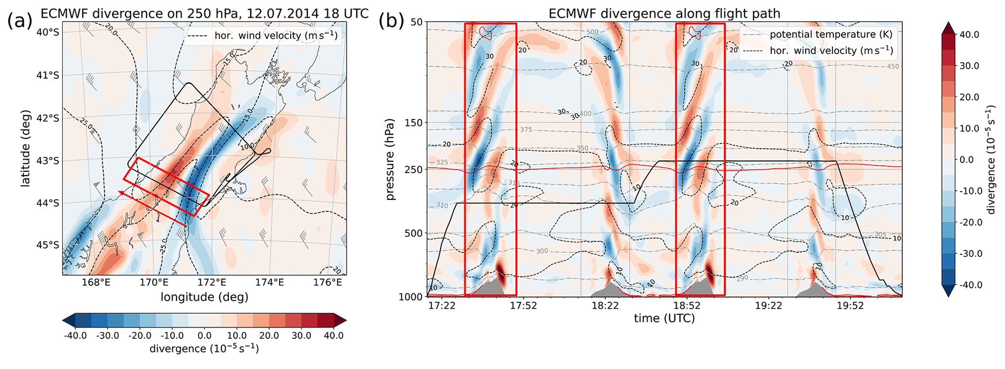
Figure 1 Divergence of the ECMWF horizontal wind during the time of flight (a) at 250 hPa and (b) as vertical cross section along the flight track indicating the signature of gravity waves over the Southern Alps. The solid red line denotes the −2 PVU isoline and the solid black line denotes the flight track. The dashed black lines denote contours of the horizontal wind velocity (10, 15, 20, 25 m s⁻¹ in (a) and 10, 20, 30 m s⁻¹ in (b)) and the dashed gray lines in (b) denote contours of potential temperature. Regions of interest are marked by red rectangles and the red arrow in (b) indicates the clockwise flight direction.

3 Observations and meteorological situation during FF09

3.1 Meteorological situation on 12 July 2014

In this study, we focus on research flight FF09 of the Falcon aircraft on the 12 July 2014 starting at 17:15 to 20:15 UTC (Fig. 1). The goal of this flight was to investigate the dynamical and chemical structure of the atmosphere in the vicinity of tropopause during a mountain wave event (Gisinger et al., 2017; Smith et al., 2016). As can be seen in Fig. 1, a rectangular pattern was flown clockwise to measure different wave responses in the northern and middle part of the Southern Island of New Zealand at two different pressure levels (330 and 260 hPa, Fig. 1), corresponding to approximately 7.9 and 10.9 km pressure altitude. The time between two vertically stacked legs at the same location was 75 min (Fig. 2).

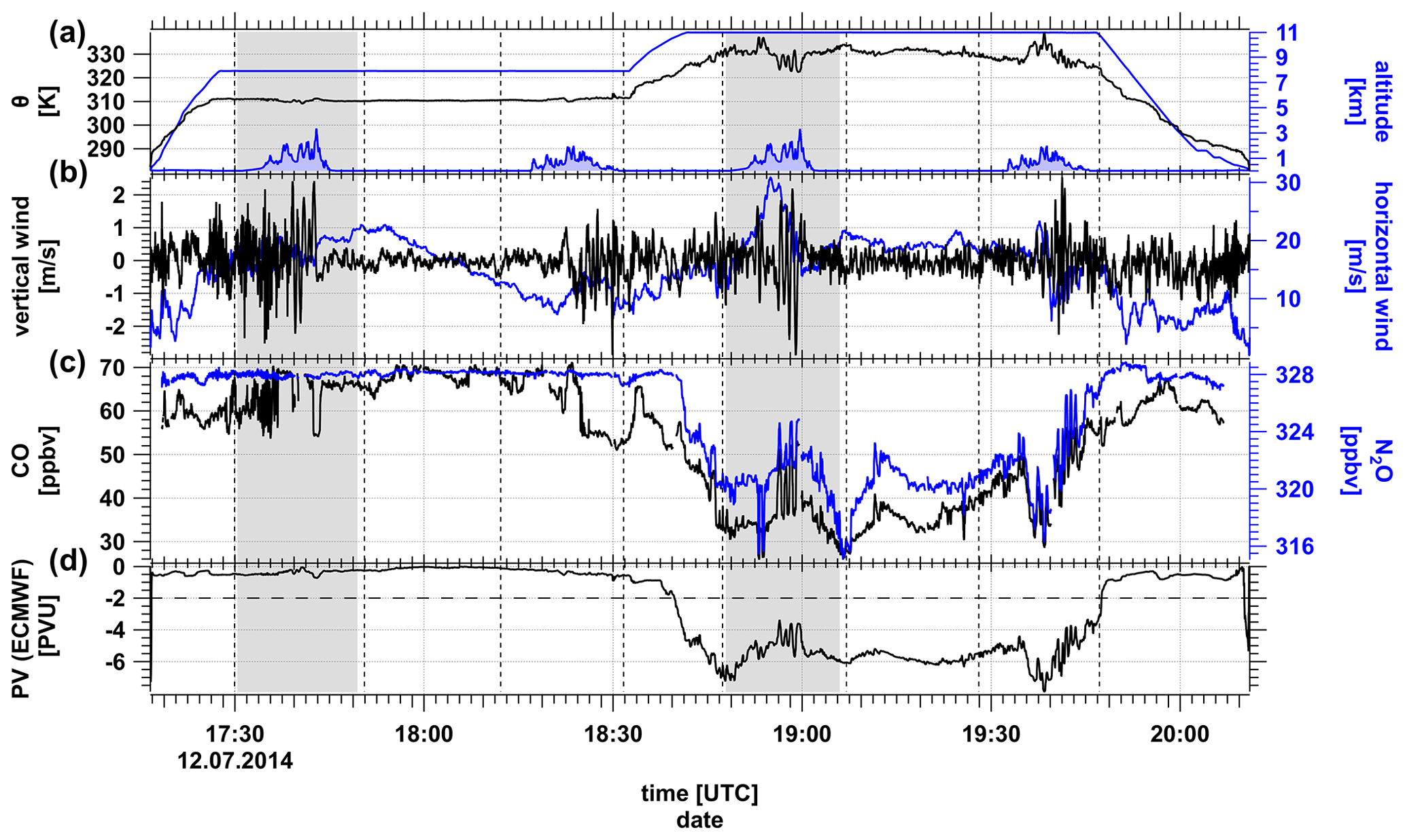
Figure 2 Time series of (a) potential temperature Θ from the measurements (black), altitude (blue) above surface elevation (filled blue), (b) vertical wind (black), horizontal wind (blue), (c) N₂O (blue) and CO (black) volume mixing ratios and (d) ECMWF potential vorticity (PV) interpolated along the flight track. Light gray boxes indicated the tropospheric and stratospheric flight section for the detailed mixing analysis. Vertical dashed lines mark turning points of the aircraft. Surface elevation was interpolated from SRTM15+ data (Tozer et al., 2019).

According to Gisinger et al. (2017), the synoptic situation can be characterized by a trough located west of New Zealand with a weak surface low located south of the islands causing northwesterly winds in the troposphere (TNW regime, Fig. 2e in Gisinger et al., 2017). In the upper level at 250 hPa at the eastern side of the approaching upper level trough, a weak gradient of the geopotential height led to a northwesterly flow with moderate horizontal winds of typically 20 m s⁻¹ along the southern flight legs (with 30 m s⁻¹ above the mountain ridge). The tropopause became relatively flat in the region and at the time of the measurements (Fig. 1b). These conditions led to the excitation of mountain waves and generated varying and moderate gravity wave responses over the South Island (Gisinger et al., 2017). Figure 1a shows the divergence of the ECMWF horizontal wind at 250 hPa at 18:00 UTC which roughly corresponds to the time of flight. The vertical cross section interpolated in time and space along the flight path shows a wave pattern above the mountain ridge indicating the excitation and propagation of orographic gravity waves, which propagate deep into the stratosphere (Fig. 1b).

It is evident from Fig. 1b that the upper flight leg at about 10.9 km is just above the dynamical tropopause. A close inspection of Fig. 1b reveals an almost constant altitude of the dynamical tropopause along the flight path without strong horizontal gradients or folds in the region of our measurements. The flat dynamical tropopause structure is mirrored by the ozone distribution from ERA5 data (not shown), which shows a rather homogeneous distribution at Θ = 330 K (approximately flight altitude) and notably also upwind of the region of our measurements.

As mentioned above, a rectangular flight pattern at two different altitudes (7.9 and 10.9 km) was chosen for the measurement of gravity waves. Here, we focus on the flight legs parallel to the wind and orthogonal to the mountains of research flight FF09.

3.2 Time series analysis of FF09

During flight FF09 on 12 July 2014, the flight legs were almost parallel to the horizontal wind and directed almost perpendicular to the Southern Alps. Pronounced fluctuations of the vertical wind occurred above the Southern Alps at each flight leg crossing the mountain ridge (Fig. 2).

The tropopause was crossed around 18:40 UTC, as indicated by the sharp decrease of the N₂O volume mixing ratio and the analyzed potential vorticity (PV) interpolated along the flight path. Particularly in the regions of strong variability of the vertical wind, Θ, N₂O and CO show enhanced variability and strong fluctuations during the stratospheric part of the flight.

The fluctuations of Θ reached an amplitude of ΔΘ = 9 K (Fig. 2). Corresponding oscillations of the vertical wind velocity reached 5 m s⁻¹ peak to peak with associated variability of N₂O in the order of 4 ppbv mirroring the oscillations of potential temperature during both flight sections parallel to the wind. These features occurred above the mountains where the meteorological analysis shows a slight altitude variability of the dynamical tropopause (−2 PVU, Fig. 1).

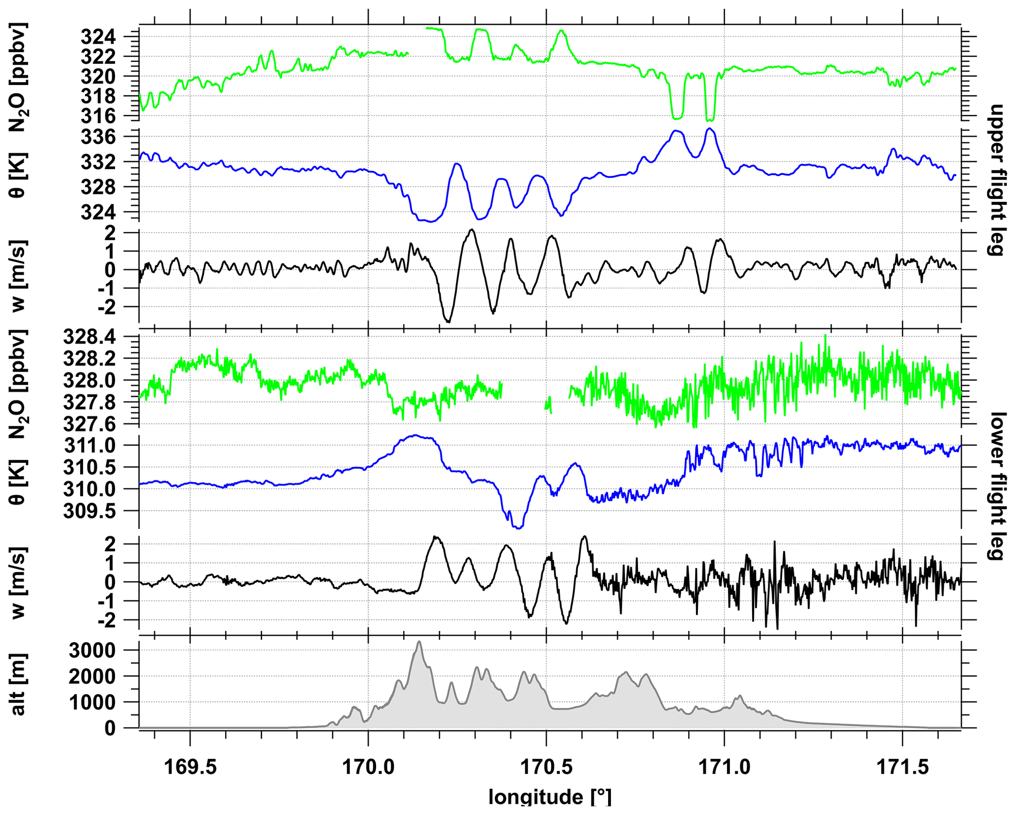
Figure 3 Cross section of the two southern stacked flight legs crossing the Southern Alps (shaded gray regions of Fig. 2) showing N₂O (green), Θ (blue) and vertical wind w (black) for the upper leg at 10.9 km (top three panels) and the lower leg at 7.9 km with surface elevation (bottom). Both legs are separated by 75 min in time. The upper leg lies in the lower stratosphere just above the tropopause, the lower leg lies in the upper troposphere.

3.3 Orographic waves during FF09

The flight sections of the two southern legs were strongly affected by orographic waves (Fig. 3). Both legs show strong fluctuations of the vertical wind component w and the potential temperature Θ with amplitudes of 2.5 m s⁻¹ and 4.5 K, respectively. The passive tracer nitrous oxide (N₂O) indicates corresponding fluctuations at the upper level in the stratosphere. At the lower level, N₂O shows a weak variability. Due to its virtually constant abundance in the troposphere, N₂O does not show corresponding oscillations to w and Θ between 170.1–170.7^∘ E. However, its variability does increase downwind of the mountains similar to w and Θ, indicating the occurrence of turbulence. At the upper level, such turbulence is not prominent, although the fluctuations of Θ, w and N₂O (Fig. 3) are indicative of at least a potential kinematic flux of N₂O, with only weakly pronounced small scale variability of w^′ (we defined the primed quantities according to Eq. 4).

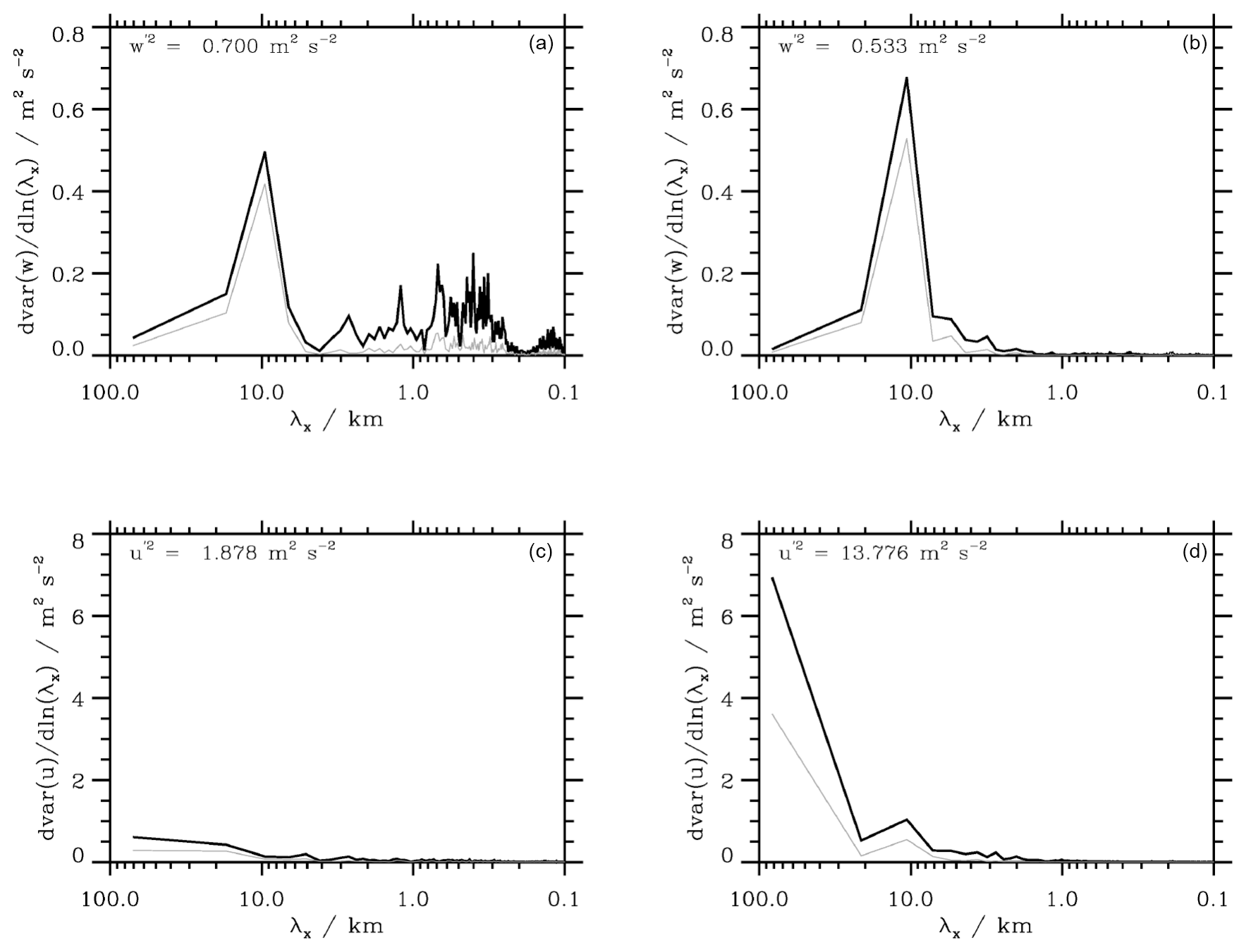
Figure 4 Binned energy spectra for the vertical wind component w (a, b) and the horizontal wind V_H (c, d) from the two southern flight legs of FF09, which crossed the mountains based on the 10 Hz data (corresponding to flight segments from 17:30–17:50 UTC and 18:47–19:07 UTC in Fig. 2). The left column shows the lower tropospheric flight track. Thick black lines are results without tapering window, thin black lines are spectra tapered with a Hanning window.

Before studying tracer transport and mixing, we analyzed the dynamical properties of the orographic waves. The binned energy spectra of the vertical wind and the horizontal wind speed V_H are shown in Fig. 4 for the southern flight legs crossing the mountains. Both legs show pronounced peaks in the w spectra at about 10 km horizontal wavelength. The vertical turbulent kinetic energy was larger in the lower leg ($\stackrel{\mathrm{‾}}{w^{\prime \mathrm{2}}}$ = 0.70 m² s⁻²) than in the upper leg ($\stackrel{\mathrm{‾}}{w^{\prime \mathrm{2}}}$ = 0.53 m² s⁻²), where the overline denotes the average over the whole 200 km flight leg. However, the energy of the lower leg seems to reside in scales smaller than about 1 km. Therefore, the spectral amplitude associated with the mountain waves at horizontal wavelengths of λ_x = 10 km is smaller at the lower leg, whereas at the upper leg, wave motions with λ_x≈ 10 km dominate. No vertical energy is found at larger scales in both legs.

The situation is different for the horizontal wind spectra where the energy is at longer horizontal scales. Only the upper leg shows a spectral peak at 10 km similar to the one in w. Thus, there are two distinct gravity wave modes: one with a long horizontal wavelength (also partly seen in V_H in Fig. 2 around 17:45 UTC) that is a response to the airflow over the whole mountain range and one with λ_x≈ 10 km. The long mode is totally absent in the lower leg and corresponds well to the rather uniform horizontal wind as shown in Fig. 2 (17:30–17:50 UTC). This long mode was probably not fully captured by the limited lengths of the legs as flown by the DLR Falcon. The other, shorter mode in the horizontal wind spectra is well-developed only in the lower leg. However, the increase of the spectral variance from the lower leg to the upper leg by a factor of 7 from 1.88 to 13.78 m² s⁻² must be mainly related to the long wave observed there according to Fig. 4.

Table 1 Wave momentum and wave energy fluxes for the two southern legs separated in upstream, downstream and across mountain side according to Fig. 6.

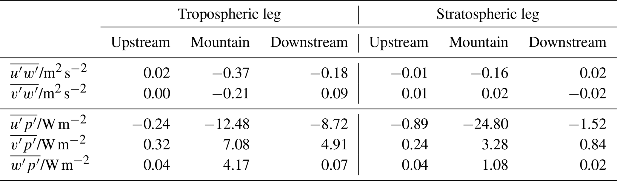
The downstream regions of the lower leg show increased variances of the vertical wind w^′ at short horizontal wavelengths. These enhanced variances might be related to the increase of small-scale energy as can be seen in the spectra shown in Fig. 4. The specific zonal momentum fluxes $\stackrel{\mathrm{‾}}{u^{\prime }{w}^{\prime }}$ (Table 1) are negative above the mountains and their magnitude is much larger than up- and downstream. This indicates a vertical upward transport of negative horizontal momentum that is characteristic of vertically propagating mountain waves.

An estimate of the vertical momentum flux divergence based on the values from the stacked flight legs,

$$\begin{array}{}\text{(3)}& -{\displaystyle \frac{\mathrm{1}}{\mathit{\rho }}}{\displaystyle \frac{\partial }{\partial z}}\stackrel{\mathrm{‾}}{\mathit{\rho }{u}^{\prime }{w}^{\prime }}\approx -{\displaystyle \frac{\partial }{\partial z}}\stackrel{\mathrm{‾}}{u^{\prime }{w}^{\prime }}={\displaystyle \frac{\partial u}{\partial t}},\end{array}$$

yields a deceleration of the zonal flow $\partial u/\partial t$ of about 6 $\mathrm{m}{\mathrm{s}}^{-\mathrm{1}}{\mathrm{d}}^{-\mathrm{1}}$. This indicates momentum deposition by dissipating mountain waves most likely occurring in the layer between the lower leg and the upper leg. The slowdown does not seem to affect the wave-induced increase of horizontal wind in the upper flight leg. Thus, the momentum dissipation must have occurred between the two flight segments separated vertically by 3000 m. This argument is supported by the small-scale signatures found in all wind components downstream of the coherent waves in the lower leg (see Figs. 2 and 3). They indicate turbulent modes associated with local instabilities above this level.

The meridional momentum fluxes $\stackrel{\mathrm{‾}}{v^{\prime }{w}^{\prime }}$ are much smaller than $\stackrel{\mathrm{‾}}{u^{\prime }{w}^{\prime }}$ (Table 1) and will not be considered here. The zonal wave energy fluxes $\stackrel{\mathrm{‾}}{u^{\prime }{p}^{\prime }}$ are negative in all segments of both legs (Table 1) and their magnitudes are largest directly over the mountains. Together with the positive vertical wave energy flux $\stackrel{\mathrm{‾}}{w^{\prime }{p}^{\prime }}$, this finding suggests vertically propagating mountain waves that travel against the mean flow, therefore, $\stackrel{\mathrm{‾}}{u^{\prime }{p}^{\prime }}$ < 0.

It is interesting to note that the vertical wave energy flux $\stackrel{\mathrm{‾}}{w^{\prime }{p}^{\prime }}$ decreases with height by a factor of 4, which means that the waves are attenuated as they propagate from the lower leg to the upper leg. This supports the idea that dissipation must have occurred in the layer between 7.9 and 10.9 km altitude. Vertical and horizontal wave energy fluxes are drastically reduced in the up- and downstream segments, indicating no significant vertical wave propagation there.

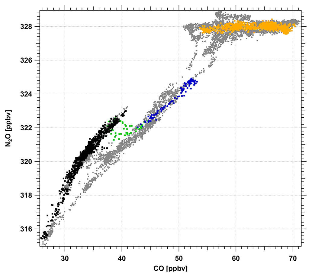
Figure 5 Scatterplot of N₂O versus CO for FF09 on 12 July 2014. The light gray points show the correlation of N₂O and CO for the whole flight. For the upper southwestern flight leg from 18:48 to 19:06 UTC in Fig. 2 (also compare Fig. 6), the data points are black, blue and green. Black colors indicate potential temperatures Θ > 328.1 K, blue for Θ < 326.3 K. The region between these two levels is marked in green. The lower leg lies entirely in the troposphere as indicated by the orange data points of N₂O = 328 ppbv.

3.4 Observation of mixing

We use tracer–tracer scatter plots of CO and N₂O to investigate if mixing occurred in the region of the enhanced wave activity. Since N₂O has no chemical sink in the atmosphere below 25 km and a lifetime of 110 years in the lower stratosphere, it is virtually homogeneously distributed in the troposphere, but exhibits a weak vertical gradient in the stratosphere (Müller et al., 2015). In contrast, CO has a chemical lifetime in the order of weeks to months in the tropopause region. Thus, it shows a sharper gradient at the tropopause. Particularly in the absence of mixing from the troposphere, CO would fall to volume mixing ratios of 10–15 ppbv given by the balance of CO production from methane oxidation and faster CO degradation by OH. Any higher value is inevitably linked to a contribution of tropospheric air. Therefore mixing, in the sense of irreversible tracer transfer, can be detected by comparing CO to any long-lived tracer with a stratospheric gradient. The approach has been extensively used to detect tropospheric influence in the stratosphere by using CO and ozone (O₃) (e.g., Hoor et al., 2002; Zahn and Brenninkmeijer, 2003; Pan et al., 2004). Here, we use N₂O instead of O₃ since it is purely controlled by atmospheric dynamics in the lower stratosphere due to the absence of local photochemical sources and sinks.

The scatter plot of CO versus N₂O for both southwesterly legs of FF09 is shown in Fig. 5. The orographic waves at the lower leg appear at almost constant N₂O volume mixing ratios of 328 ppbv. This is due to the fact that in the troposphere, no gradients of N₂O are present. Therefore, mixing does not change the N₂O volume mixing ratio as long as no stratospheric air is involved. Thus we cannot diagnose mixing for the lower leg on the basis of tracer–tracer correlations.

Figure 6 Time series of potential temperature Θ and N₂O for the flight leg around 18:48–19:00 UTC just above the tropopause over the mountain. Colors indicate two different layers of air masses (black, blue) and a mixed layer in between (green) corresponding to Fig. 5. Vertical lines mark the upstream (< 170^∘ E), above mountain (170–171^∘ E), and downstream side (> 171^∘ E).

However, for the stratospheric legs across the mountain ridge during FF09, the scatter plot clearly shows different chemical regimes in the stratosphere (i.e., for N₂O < 326 ppbv, Fig. 5) as indicated by the two different branches of the two tracers. These two branches indicate two distinct air masses within the lower stratosphere which differ in their chemical composition as evident by the different N₂O volume mixing ratios. A detailed analysis (see Fig. 6) shows that the two branches of the correlation can be assigned to two distinct potential temperature intervals which correspond to two layers of different chemical composition for Θ > 328.1 K and Θ < 326.3 K. Notably, the data points (marked in green) which fall between the two data clouds (N₂O < 324 ppbv) forming two compact branches (and thus isentropes as given above) connect both air masses. The intermediate points thus mark a layer between 326.3 K < Θ < 328.1 K, where the tracer–tracer diagram indicates mixing between the two branches (green squares in Fig. 5).

To put the stratospheric part (i.e., for N₂O < 327 ppbv) of the tracer–tracer data of the scatter plot in a geophysical and meteorological context, Fig. 6 shows the time series of potential temperature and N₂O color coded according to the regimes identified from the scatterplot (Fig. 5). The two branches of the correlation can be clearly assigned to different isentropes separating air masses with different chemical composition. Notably, those points which indicate mixing in the tracer-tracer scatterplot fall between the distinct layers. As evident from Fig. 6, the region where the chemical composition indicates mixing (green) corresponds to the occurrence of waves as indicated by strong fluctuations of the vertical wind and potential temperature. Therefore, we hypothesize that mountain-wave-induced mixing must have occurred in the stratosphere leading to the observed tracer variability as shown above. In the following section, we will therefore focus on the stratospheric flight section across the mountains from 18:48 to 19:06 UTC as indicated by the gray box in Fig. 2 if not noted differently.

4 Analysis of cross-isentropic mixing

Kinematic fluxes on the basis of the covariance of vertical wind and tracer variability $w^{\prime }{\mathit{\chi }}^{\prime }$ might provide information on the local vertical fluxes. For a correct estimate of an irreversible flux, one needs to calculate the flux divergence (Shapiro, 1980). However, this would require simultaneous measurements of the tracer of interest on two closely stacked vertical levels, which cannot be accomplished with one aircraft (as was the case here). A comparison of the local fluxes for the stacked levels is in principle possible. However, due to the large vertical spacing of 3 km, the potential influence from large-scale horizontal advection could strongly impact the flux divergence estimates between the two flight levels.

Adiabatic vertical displacements of air masses may simultaneously displace the location of isentropes and tracer isopleths, which therefore does not lead to irreversible tracer transport and mixing at a given location downwind of a mountain ridge (i.e., $\partial \mathit{\chi }/\partial \mathrm{\Theta }$ = const, Moustaoui et al., 2010). In contrast, cross-isentropic (= diabatic) fluxes must change cross-isentropic gradients of species (i.e., $\partial \mathit{\chi }/\partial \mathrm{\Theta }$) with respect to potential temperature. Therefore, a change of tracer gradient (i.e., $\partial {\mathrm{N}}_{\mathrm{2}}\mathrm{O}/\partial \mathrm{\Theta }$; similar to Balluch and Haynes, 1997) as a function of Θ downwind of the mountain is indicative of irreversible cross-isentropic tracer exchange which might have occurred above the mountain ridge. In a Lagrangian sense, the occurrence of turbulence and turbulent mixing acts as a source of tracer at a given isentrope, if the background tracer gradient changes with height in the inflow region (e.g., at the tropopause). We therefore investigated whether tracer gradients with respect to potential temperature Θ were changed due to the occurrence of gravity-wave-induced turbulence leading to cross-isentropic mixing by comparing local tracer profiles upstream and downstream of the mountains ($\partial \mathit{\chi }/\partial \mathrm{\Theta }{\mathrm{|}}_{\text{up}}\ne \partial \mathit{\chi }/\partial \mathrm{\Theta }{\mathrm{|}}_{\text{down}}$).

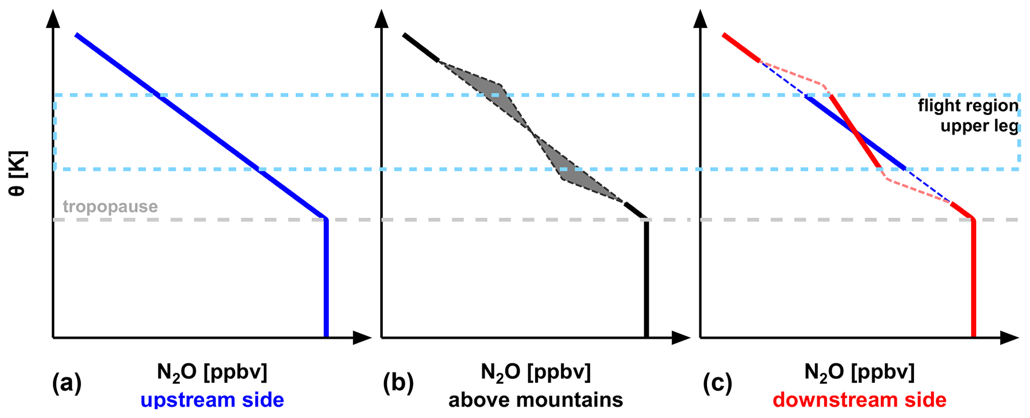
Figure 7 Schematic evolution of potential temperature Θ versus N₂O in the presence of cross-isentropic mixing at the tropopause (e.g., by orographic-wave-induced turbulence). The blue curve (a) shows the situation on the upstream side. The relation between N₂O and Θ (blue) is modified by mixing (b; dotted black and shaded gray) over the mountains leading to a modified profile on the downstream side (c; red) compared to the original upstream relation (blue). The dashed gray line shows the tropopause and the dashed light blue rectangle the flight region of the upper leg.

In particular, the gradient change of the conservative tracer N₂O at the tropopause is perfectly suited to test our hypothesis that gravity-wave-induced turbulence led to cross-isentropic mixing. Since N₂O in the lowermost stratosphere is not affected by local chemistry, it is purely under dynamical control. At the tropopause, N₂O exhibits a change of the vertical gradient with respect to Θ ($\partial {\mathrm{N}}_{\mathrm{2}}\mathrm{O}/\partial \mathrm{\Theta }$).

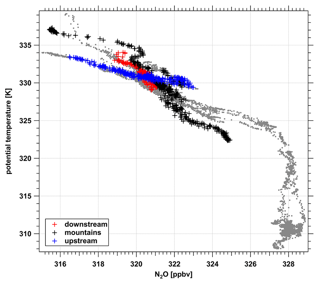
Figure 8 Profile of N₂O during FF09 (gray) as a function of potential temperature Θ. The upper leg of the southwestern part is shown with different colors, indicating different flight sections along the flight leg (blue: upstream, red: downstream, black: above the mountains, comp. Fig. 6).

The decrease of N₂O in the lowermost stratosphere with respect to Θ is schematically shown in Fig. 7. For the following analysis, we will use the following conventions: we will express the slope as ratio of the anomalies ${\mathrm{\Theta }}^{\prime }/{{\mathrm{N}}_{\mathrm{2}}\mathrm{O}}^{\prime }$ (according to Eq. 4) to be consistent with the profile view (as in Figs. 7 and 8). We will apply this convention with Θ in the numerator and N₂O in the denominator throughout the following analyses. We will further use the terminology below.

The term Θ–N₂O relation refers to general aspects of their relation, the term ${\mathrm{\Theta }}^{\prime }/{{\mathrm{N}}_{\mathrm{2}}\mathrm{O}}^{\prime }$ ratio (associated with a slope) will be used when referring to the specific measurements. A change of this ratio is directly linked to the change of the vertical gradient with respect to Θ ($\partial {\mathrm{N}}_{\mathrm{2}}\mathrm{O}/\partial \mathrm{\Theta }$).

A schematic of our hypothesized relation of Θ and N₂O is shown in Fig. 7 which shows the evolution of the N₂O profile for a flow over a mountain assuming an effect of gravity-wave-induced cross-isentropic mixing on the N₂O profile. The upstream side represents the unperturbed background N₂O profile. Above the mountain, orographic-wave-induced turbulence may occur which could potentially change the vertical gradient of N₂O with respect to Θ at the tropopause. This effect of irreversible mixing is schematically depicted by the gray shading in Fig. 7. Since $\partial {\mathrm{N}}_{\mathrm{2}}\mathrm{O}/\partial \mathrm{\Theta }$ changes at the tropopause, the upstream relation between Θ and N₂O can be modified by turbulent mixing which will change the relation of the N₂O profile with respect to Θ. As a result of the irreversible diabatic process, the downstream side shows the modified profile of N₂O compared to the upstream region (red versus blue slope).

Thus, in the case of gravity-wave-induced turbulent mixing during flight FF09, we expect a more rapid decrease of N₂O with increasing Θ in the inflow region upwind the mountains than at the downstream side of the mountain ridge as an effect of turbulent mixing. The vertical N₂O profile with respect to Θ is modified from upstream to downstream due to turbulent mixing.

Figure 8 shows the measured N₂O profile as a function of potential temperature Θ for the entire flight FF09. The colored data points denote different longitudes relative to the mountain ridge to separate the inflow, across mountain, and downstream part of the flight leg (see Fig. 6). As evident from Fig. 8, different relations between Θ and N₂O appear on the upstream side, downstream side and above the mountains. The different relations are consistent with our hypothesis that the relationship between Θ and N₂O (and consequently the vertical gradient $\partial {\mathrm{N}}_{\mathrm{2}}\mathrm{O}/\partial \mathrm{\Theta }$) will be changed in regions impacted by gravity-wave-induced mixing. Upstream of the mountains this Θ–N₂O relation shows a strong decrease of N₂O with increasing Θ and a compact relationship (i.e., a well-defined relationship exhibiting only weak scatter). On the downstream side, the N₂O decrease with respect to Θ is much weaker with intermediate values and larger variability above the mountains (see Fig. 8).

4.1 Scale analysis

In a next step, we performed a scale-dependent correlation analysis as described below to further analyze the impact of the orographic waves on the Θ–N₂O relation and to account for a potential effect of different scales of the waves on cross-isentropic mixing. For this, we applied a Reynolds decomposition and separated the data into a mean part $\stackrel{\mathrm{‾}}{\mathit{\chi }}$ and a perturbation part χ^′ (as well as $\stackrel{\mathrm{‾}}{\mathrm{\Theta }}$ and Θ^′):

$$\begin{array}{}\text{(4)}& \mathit{\chi }\left(t\right)=\stackrel{\mathrm{‾}}{\mathit{\chi }}+{\mathit{\chi }}^{\prime }\left(t\right)\iff {\mathit{\chi }}^{\prime }\left(t\right)=\mathit{\chi }\left(t\right)-\stackrel{\mathrm{‾}}{\mathit{\chi }}.\end{array}$$

The mean $\stackrel{\mathrm{‾}}{\mathit{\chi }}$ is calculated with a boxcar average which works as a low-pass filter and removes high-frequency variability. We analyzed the data for different averaging periods to account for varying perturbation wavelengths and at different scales using the following formula:

$$\begin{array}{}\text{(5)}& \stackrel{\mathrm{‾}}{\mathit{\chi }}={\displaystyle \frac{\mathrm{1}}{t_{\mathrm{2}}-t_{\mathrm{1}}}}\underset{t_{\mathrm{1}}}{\overset{t_{\mathrm{2}}}{\int }}\mathit{\chi }\left(t\right)\mathrm{d}t,\end{array}$$

where t₂−t₁ is the integration width.

Above the tropopause, Θ increases while N₂O decreases. Thus, we expect an anti-correlation for the perturbations of these two quantities, Θ^′ and N₂O^′, with a given slope (or ${\mathrm{\Theta }}^{\prime }/{{\mathrm{N}}_{\mathrm{2}}\mathrm{O}}^{\prime }$ ratio) in the inflow region upstream of the mountains. For linear non-dissipative waves, the ${\mathrm{\Theta }}^{\prime }/{{\mathrm{N}}_{\mathrm{2}}\mathrm{O}}^{\prime }$ ratio will therefore remain constant for different integration widths. In the presence of non-conservative dissipative processes, the linear relation between Θ^′ and ${{\mathrm{N}}_{\mathrm{2}}\mathrm{O}}^{\prime }$ and thus their ratio will change as explained above.

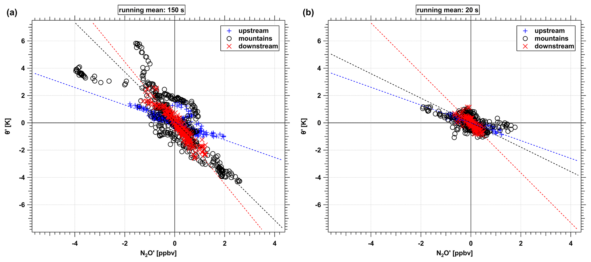
Figure 9 Relation between Θ^′ and ${{\mathrm{N}}_{\mathrm{2}}\mathrm{O}}^{\prime }$ for upstream (blue), downstream region (red) and above mountains (black). (a) Averaging period of 150 s (32.5 km). (b) Averaging period of 20 s (4.3 km). The dotted lines indicate the slopes of the different flight segments. Note the changing slope over the mountains.

As an example, the effect of different integration intervals on the distribution of data points is shown in Fig. 9 for two different interval lengths. The applied fit accounts for errors in x and y directions (Press et al., 1987). The figure shows the same subset of data using averaging periods of 150 s (Fig. 9a) and 20 s (Fig. 9b) corresponding to a horizontal scale of 33 and 4 km, respectively. For wavelengths shorter than these dimensions, the ratios at the downstream (red) and upstream (blue) side only slightly change. Both however clearly show an increased ratio at the downstream side (red) compared to the upstream (blue).

Above the mountains (black), the relation is perturbed, showing a high variability. The above-mountain ratio for the long waves (i.e., averaging periods, Fig. 9a) is closer to the downstream side compared to the shorter wavelengths (Fig. 9b).

Figure 10 Scale-dependent correlation anomaly analysis for different integration times showing the ${\mathrm{\Theta }}^{\prime }/{{\mathrm{N}}_{\mathrm{2}}\mathrm{O}}^{\prime }$ ratio for different averaging periods (i.e., wavelengths) for upstream (blue), downstream (red) and above mountains (black).

To account for different scales and thus increasing wavelengths, we subsequently increased the averaging period in steps of 1 s from 2–292 s (length of the shortest data segment unbroken by calibrations). The corresponding development of the ${\mathrm{\Theta }}^{\prime }/{{\mathrm{N}}_{\mathrm{2}}\mathrm{O}}^{\prime }$ ratios is shown in Fig. 10. The blue curve is deduced from the data in the upstream region. With a value of about −0.6 K ppbv⁻¹ the ratio is almost constant over all averaging periods. This indicates that no cross-isentropic mixing perturbs the upstream linear ${\mathrm{\Theta }}^{\prime }/{{\mathrm{N}}_{\mathrm{2}}\mathrm{O}}^{\prime }$ ratio at any wave period.

Indeed, in the long scale limit, a clear separation for the downstream and above-mountain ratio is evident. The black and red curves show a ${\mathrm{\Theta }}^{\prime }/{{\mathrm{N}}_{\mathrm{2}}\mathrm{O}}^{\prime }$ ratio change for different averaging periods. Above the mountains, the ${\mathrm{\Theta }}^{\prime }/{{\mathrm{N}}_{\mathrm{2}}\mathrm{O}}^{\prime }$ ratio starts to change at longer averaging periods (100 s, 21.6 km) compared to the downstream side. The changes at the downstream side start at shorter averaging periods (40 s, 8.7 km), indicating smaller scales or wavelengths relevant for the change of the ${\mathrm{\Theta }}^{\prime }/{{\mathrm{N}}_{\mathrm{2}}\mathrm{O}}^{\prime }$ ratio. Downstream and above-mountain ${\mathrm{\Theta }}^{\prime }/{{\mathrm{N}}_{\mathrm{2}}\mathrm{O}}^{\prime }$ ratios merge for longer periods to the new (modified) gradient with a ${\mathrm{\Theta }}^{\prime }/{{\mathrm{N}}_{\mathrm{2}}\mathrm{O}}^{\prime }$ ratio around 2 K ppbv⁻¹.

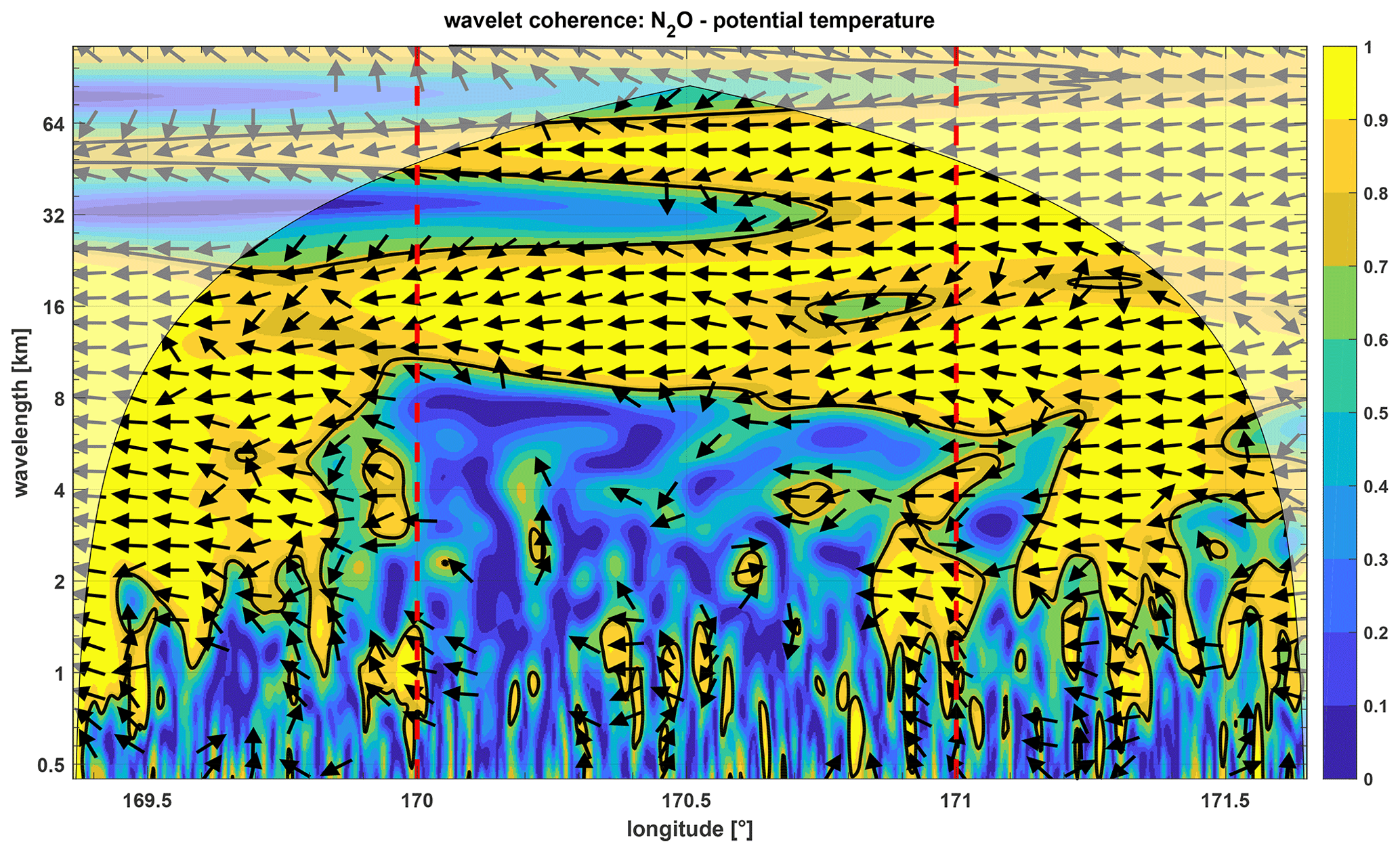
Figure 11 Wavelet coherence of N₂O and potential temperature (wavelength = period ⋅ flight speed (216 m s⁻¹), see Eq. 2). Arrows to the left indicate that N₂O and potential temperature are shifted by 180^∘. In regions with a coherence lower than 0.5, the phase indication is removed. The shaded region marks the cone of influence, where edge effects affect the analysis. The solid lines show the 95 % confidence level as given in Sect. 2.4. Yellow colors indicate a high coherence and blue colors indicate a low coherence. Vertical lines mark the upstream, above mountain, and downstream side.

Similar to Alexander and Pfister (1995), we used the upstream relation between Θ and N₂O to estimate the N₂O amplitude which one would expect if only adiabatic transport by the gravity waves over the mountain would occur. The observed peak-to-peak variability of Θ of 8 K (Fig. 6) would correspond to N₂O = 13 ppbv, while only 4 ppbv are observed consistent with an impact of diabatic mixing processes changing the upstream relation.

In summary, the ratio-changing behavior would be consistent with a modification of the initial upstream N₂O profile across the mountains, where the relation between Θ and N₂O is perturbed. When crossing the mountain ridge, gravity-wave-induced turbulence affects the Θ–N₂O relation with a persistent effect at the downstream side. The downstream impact is evident from the different ${\mathrm{\Theta }}^{\prime }/{{\mathrm{N}}_{\mathrm{2}}\mathrm{O}}^{\prime }$ ratio at larger wavelengths at the downwind side compared to the upstream ratio. Therefore, we conclude that during FF09, mountain waves modified the ${\mathrm{\Theta }}^{\prime }/{{\mathrm{N}}_{\mathrm{2}}\mathrm{O}}^{\prime }$ ratio by the generation of turbulence at small scales. They induced cross-isentropic turbulent mixing leading to changes at large scales downwind of the Alps as evident from the ${\mathrm{\Theta }}^{\prime }/{{\mathrm{N}}_{\mathrm{2}}\mathrm{O}}^{\prime }$ ratio and finally the vertical gradient $\partial {\mathrm{N}}_{\mathrm{2}}\mathrm{O}/\partial \mathrm{\Theta }$ (Fig. 6).

To identify the leading spatial and temporal scales for the cross-isentropic (i.e., irreversible) mixing of N₂O, we analyzed the wavelet coherence between the time series of N₂O and Θ in Fig. 11. Coherence is a measure of the intensity of the covariance of 2 time series. At the upstream side (< 170^∘ E), there is mostly high coherence according to the fact that Θ and N₂O co-vary across different timescales from 1.7–17.3 km (corresponding to 8–80 s). Further, the phase relation between the time series of N₂O and Θ (see Fig. 6) is almost constant at 180^∘ for scales < 20 km, which one would expect for opposing vertical gradients of N₂O and Θ in the stratosphere. Thus, both the wavelet coherence and the phase relation confirm the finding of the absence of mixing from the previous upwind slope analysis (Fig. 10, upstream side).

Above the mountains (from 170 to 171^∘ E), there is low coherence with values lower than 0.7 for timescales < 8,7 km (< 40 s) accompanied by a breakdown of the phase relation between N₂O and Θ, both indicating a decrease of the covariance. On the downstream side (from 171^∘ E), especially at small periods, higher coherence values and defined phase relations re-establish compared to the above-mountain regime, albeit more variable than at the upstream side. Consistent with Fig. 10, in upwind regimes with a high coherence, N₂O and the potential temperature Θ co-vary: the phase relation between them remains constant across scales and the calculated slope (Fig. 10) is unchanged too. Above the mountains, the phase relation breaks down due to cross-isentropic mixing, especially for wave periods smaller than 6.5 km (30 s). Downwind, a new ratio re-establishes as a result of mixing above the mountain ridge, but with a defined phase relation again and different ratios.

Figure 12 (a) Co-spectrum of the cross-wavelet transformation of N₂O and vertical wind. The shaded region marks the cone of influence in which edge effects play a role. The black contour lines indicate 5 % significance levels against red noise. Red colors denote a positive flux and blue colors indicate a negative flux. (b) Scale-averaged wavelet co-spectrum over all periods.

We therefore conclude that above the mountains, the low coherence and the breakdown of the phase relationship at short wavelength were an effect of the gravity waves which produced turbulence and led to cross-isentropic mixing. Therefore, the change in the ${\mathrm{\Theta }}^{\prime }/{{\mathrm{N}}_{\mathrm{2}}\mathrm{O}}^{\prime }$ ratio from the upwind to the downwind side is the result of gravity-wave-induced mixing. Since the mixing is cross-isentropic, this changed the ${\mathrm{\Theta }}^{\prime }/{{\mathrm{N}}_{\mathrm{2}}\mathrm{O}}^{\prime }$ ratio, which is evident at the downstream side, where a modified ratio establishes (compared to the upwind side).

4.2 Fluxes

To estimate quantitative tracer fluxes, we use the co-spectrum of the cross-wavelet transformation between the vertical wind w and N₂O (see Sect. 2.4). Unlike other methods, the wavelet analysis has the advantage to resolve wave-induced processes in space and time.

The wavelet co-spectrum is calculated from the real part of the cross-wavelet transformation and gives the spectral contributions of vertical fluxes (Mauder et al., 2007). Figure 12 shows the co-spectrum of the cross-wavelet transformation of N₂O and vertical wind w for the higher flight level during FF09. There are two regions with enhanced fluxes within the 5 % significance level (solid black line), which are both located above the mountains (compare Fig. 2). The first region is between 170.0 and 170.6^∘ E, the second between 170.8 and 171.0^∘ E. The first region shows mainly positive trace gas fluxes with values up to 0.50 ppbv m s⁻¹ at wavelengths ranging from 8–16 km, corresponding to the vertical wind energy maximum around λ_x = 10 km Fig. 4. The second region exhibits upward and downward fluxes at slightly shorter scales from about 3–16 km. Here, the strongest fluxes have values from about −0.22 to +0.56 ppbv m s⁻¹. The fluxes in both regions are co-located to enhanced wave occurrence above the mountains, as seen in Figs. 6 and 2.

Since ozone was measured with a temporal resolution of 10 s, we did not directly determine ozone fluxes in the present case. To give an estimate of the associated ozone flux, we can use the N₂O–O₃ correlation slope, which is about −20 ppbv (O₃)$/$ppbv (N₂O) for the Southern Hemisphere in July (Hegglin and Shepherd, 2007). This results in a negative flux of O₃ of 10 ppbv m s⁻¹ for the positive N₂O-fluxes.

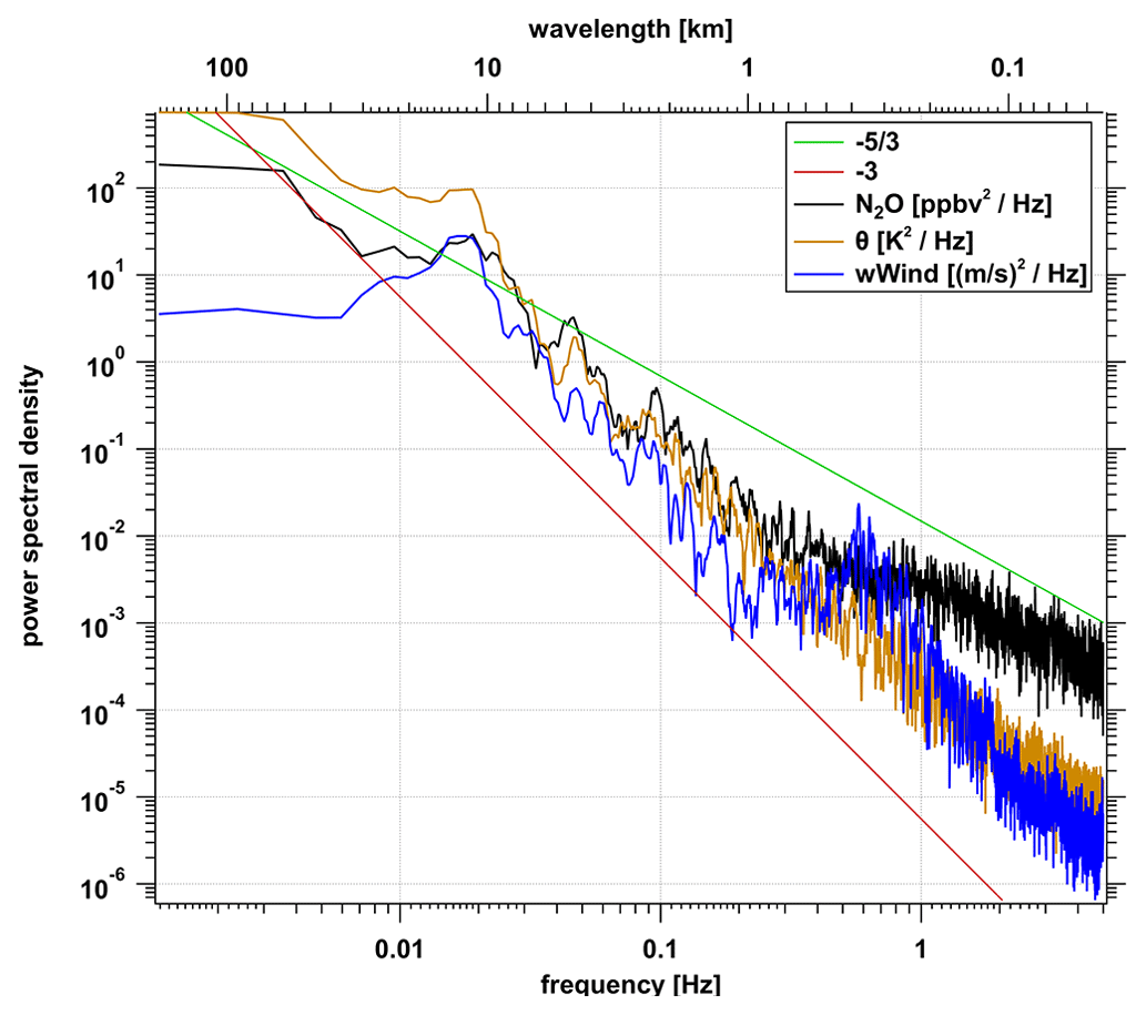
Figure 13 Power spectral density of vertical wind (blue), potential temperature (orange) and N₂O (black) for the flight segment above the mountains. The power spectral density has been smoothed by a boxcar average of 5 s. The green and red reference lines have slopes of −5$/$3 and −3.

4.3 Turbulence occurrence

The power spectral density (PSD) for Θ and the vertical wind component w in Fig. 13 show a slope of −3 for wavelengths longer than 721 m (< 0.3 Hz), in agreement with the observations of airborne measurements during START08 (2008 Stratosphere–Troposphere Analyses of Regional Transport; Zhang et al., 2015) for wavelengths < 10 km. For shorter wavelengths (i.e., higher frequencies), the increase of the PSD at 433 m (0.5 Hz) would be consistent with a potential source of turbulent energy above the mountains. Notably, a similar peak of the PSD of w was observed during the START08 campaign for some flight sections in regions of turbulence occurrence over the Rocky Mountains (Zhang et al., 2015). However, the peak of the PSD from the vertical wind component around 433 m (0.5 Hz) could also correspond to oscillations caused by the autopilot of the aircraft (Schumann, 2019). They report oscillations with wavelengths of 6.7 km in regions of high turbulence, which is a factor of 10 longer than in our case. Thus, an artificial non-atmospheric origin of the peak cannot be completely ruled out.

For wavelengths below 108 m (> 2 Hz), the slope of the PSD of both w and Θ approach −5$/$3, which can be related to isotropic turbulence. Figure 13 also shows the PSD of N₂O. It has a slope of −3 for longer wavelengths (smaller frequencies) and a flattening slope for wavelengths smaller than 721 m (> 0.3 Hz). A change of the turbulent behavior as indicated by the transition of PSD slopes occurs in the wavelength range between 271 to 721 m (corresponding to 0.8 to 0.3 Hz), where the PSD of the vertical wind indicates a source of turbulent energy. Notably, the PSD of N₂O points to a turbulent behavior for small wavelengths and thus the occurrence of turbulent fluxes corresponding to the analysis in the previous section.

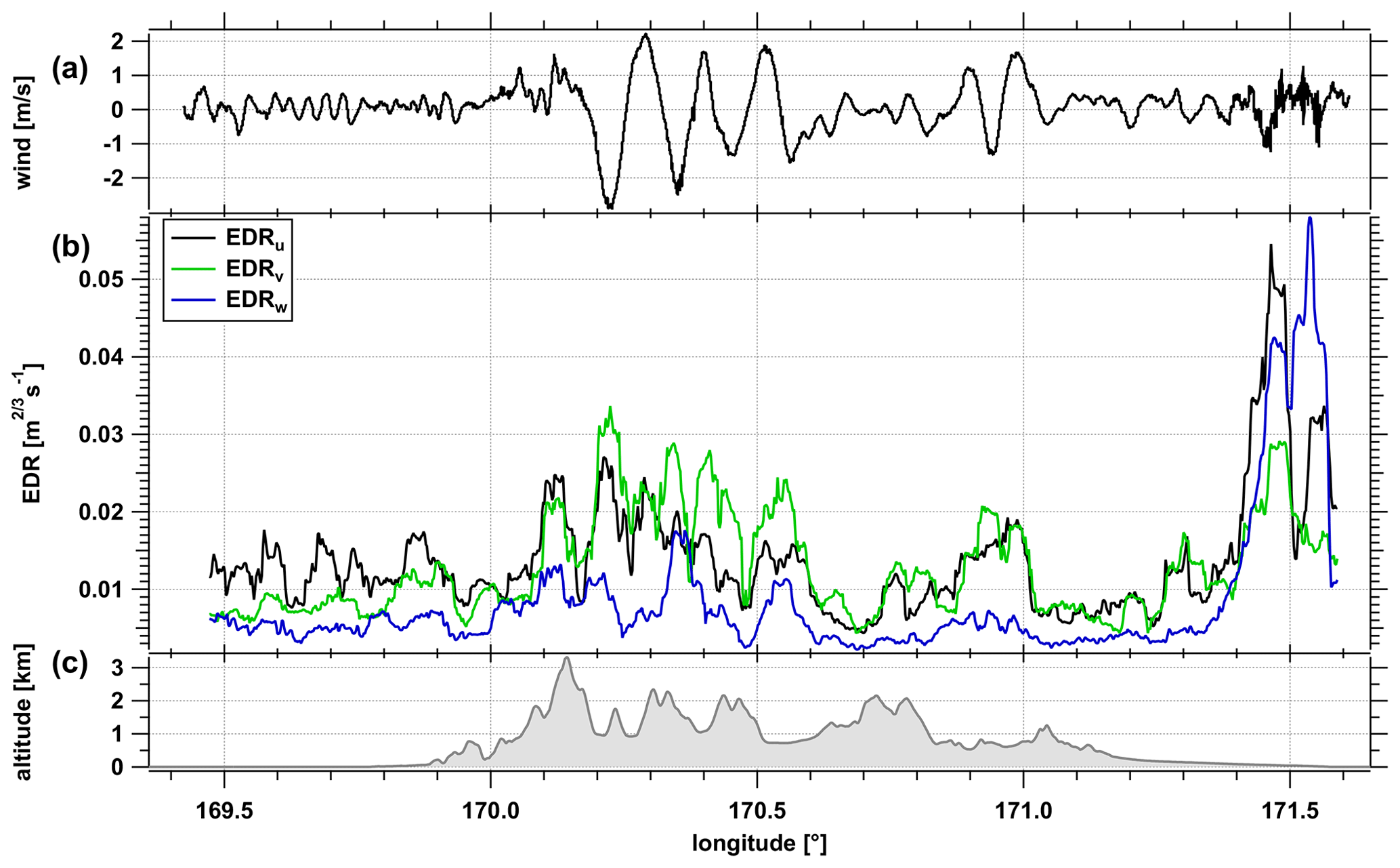
Figure 14 Time series of (a) vertical wind, (b) EDR for the measured wind components for the upper flight leg indicating weak, but non-vanishing turbulence during the time of flight above the Southern Alps (orography shown in c).

Further support for our hypothesis that mountain wave induced turbulence perturbed the N₂O profile comes from the analysis of the cube root of the eddy dissipation rate EDR = ${\mathit{ϵ}}^{\mathrm{1}/\mathrm{3}}$ from the measured three-dimensional winds. For this analysis, we used the method by Bramberger et al. (2018) to calculate the EDR for the three wind components as measured by the aircraft (Fig. 14). Above the mountains, the oscillations of the vertical wind velocity w indicate the region of mountain wave occurrence. The EDR over the mountains appears to be weak below the threshold of light turbulence of about 0.05 ${\mathrm{m}}^{\mathrm{2}/\mathrm{3}}{\mathrm{s}}^{-\mathrm{1}}$ (Bramberger et al., 2018). However, the values of EDR_u,v for the horizontal wind components are enhanced over the mountain. In the lee of the mountains, the EDR of all wind components is enhanced. Further support for our hypothesis and our results comes from the analysis of the occurrence of mountain-wave-induced turbulence using the Graphical Turbulence Guidance (GTG) with ECMWF operational analysis data (Bramberger et al., 2018; Sharman et al., 2006; Sharman and Pearson, 2017). The GTG analysis matches the observed locations of wave occurrence during the flight and the regions of strong variability of the vertical wind (not shown). Though the values are too high, this supports the conclusion that turbulence occurred in the region of the mixing events, either shortly before or during the measurements.

The weak EDR at the upper flight leg in accordance with the weak turbulence occurrence as opposed to the lower leg (see Fig. 4) may be explained by the time difference between the two legs. As evident from the wave analysis, orographic waves were crossed during the first leg and led to wave breaking and momentum deposition in the region between the legs. At the higher leg, only a weak turbulence signal remained 1 h later when the second crossing took place. The change of $\partial \mathrm{\Theta }/\partial$N₂O is a unique indication of a diabatic process, which must have changed the gradient from the upstream to the downwind side exactly above the mountains. The evidence for strong orographic wave activity at the lower level that propagates to the 10.9 km level serves as the only plausible explanation for these observations. The fact that the turbulence is weak during the time of flight at the higher level must be attributed to the time shift between the two flight legs and the high intermittency of turbulence.

5 Conclusions

We present an analysis of high-resolution N₂O measurements in the region of orographic gravity waves over the Southern Alps in New Zealand during the DEEPWAVE 2014 campaign. These gravity waves led to diabatic trace gas fluxes and a persistent local effect on the composition downwind of the mountain and the above the tropopause.

The spectral analysis of the wind components measured along two vertically stacked levels indicates dissipation of momentum by orographic waves above the mountains between these levels and the generation of turbulence. The spectral energy of the vertical wind component shows strong signals at short horizontal wavelengths (< 1 km) at the lower flight leg at 7.9 km. At the higher leg, which was flown 75 min later in the stratosphere, horizontal wavelengths of 10 km dominate the energy spectrum of w^′ with much weaker contribution at the shorter scale. Corresponding to the fluctuations of the vertical wind and potential temperature Θ, strong fluctuations of the tracer N₂O were also observed at the upper flight leg in the region of the occurrence of orographic waves. Based on the analysis of the CO–N₂O relationship, we could identify mixing between two layers of different air masses in the tropopause region. Upstream and downstream of the mountain, different vertical gradients of N₂O with respect to potential temperature Θ were observed and enhanced variability of this gradient was observed above the mountains. Since N₂O is chemically inert, a change of the N₂O–Θ relation must be due to cross-isentropic mixing effects.

A scale-dependent slope analysis shows that mixing was initiated over the mountain ridge with reversible displacements of tracer isopleths and Θ. These fluctuations must have perturbed the compact relation between Θ and N₂O via the generation of turbulence and thus irreversible turbulent cross-isentropic mixing.

Mountain-wave-induced mixing is also consistent with the indication for wave breaking and momentum deposition above the mountains between the two flight legs. Noting that the stratospheric flight leg was flown 75 min after the lower leg explains why the turbulent kinetic energy for w^′ at short horizontal wavelengths is rather small compared to the lower leg. Still, the power spectral energy spectra of N₂O and Θ with slopes of −5$/$3 at the smallest scales can be seen as the result of the turbulence that may have occurred on this level.

The tracer distribution conserves the effect of prior occurrence of highly transient turbulence occurrence. At the downstream side, a modified compact N₂O–Θ relation establishes as a result of the wave-induced turbulence above the mountains. The reversible air mass displacements induced by the gravity waves are similar to the mechanism described in (Moustaoui et al., 2010; Mahalov et al., 2011). This behavior is confirmed by cross-wavelet analyses showing a breakdown of the coherence and phase relationship between N₂O and Θ over the mountains.

The vertical fluxes of N₂O are estimated to be 0.5 ppbv m s⁻¹, corresponding to negative fluxes of O₃ of approximately 10 ppbv m s⁻¹.

The change of the Θ–N₂O relation from the upstream to the downstream side over the mountain ridge is a unique indicator for cross-isentropic (i.e., irreversible) turbulent exchange of species, which was initiated by the orographic waves. The fact that the modified relationship prevails downstream of the mountain shows that the turbulence associated with the orographic waves was associated with cross-isentropic mixing. The approach using the Θ–N₂O relation notably differs from local covariance analysis of vertical winds and tracers since it shows that at least part of the kinematic fluxes contributed to a cross-isentropic component.

Diabatic trace gas fluxes are key for understanding the effect of mixing processes on the large-scale composition of the UTLS where they contribute to the mixing-induced uncertainty of radiative forcing estimates (Riese et al., 2012). Though the occurrence of orographic waves has strong seasonality and a high degree of transience (Fritts and Alexander, 2003; Rapp et al., 2021), regions of gravity wave activity are hotspots for turbulence at the tropopause (Alexander and Grimsdell, 2013; Fritts and Alexander, 2003). Our data show that gravity-wave-induced turbulence can have a persistent effect on the distribution of species and thus a potential forcing impact of radiatively active tracers by changing their isentropic gradients. By subsequent isentropic transport as part of the stratospheric flow, the impact of radiatively active traces has a strong non-local component downwind of the mountains. Thus, gravity-wave-induced mixing contributes to the overall mixing-induced uncertainty of radiative forcing (Riese et al., 2012).