Global impact of the COVID-19 lockdown on surface concentration and health risk of atmospheric benzene

To curb the spread of the COVID-19 pandemic, many countries around the world imposed an unprecedented lockdown, producing reductions in pollutant emissions. Unfortunately, the lockdown-driven global ambient benzene changes still remain unknown. An ensemble machine-learning model coupled with chemical transport models (CTMs) was applied to estimate global high-resolution ambient benzene levels. Afterwards, the extreme gradient boosting (XGBoost) algorithm was employed to decouple the contributions of meteorology and emission reduction to ambient benzene. The change ratio (P_dew) of the deweathered benzene concentration from the pre-lockdown to lockdown period was in the order of India (−23.6 %) > Europe (−21.9 %) > the United States (−16.2 %) > China (−15.6 %). The detrended change (P^∗) of the deweathered benzene level (change ratio in 2020 − change ratio in 2019) followed the order of India ($P^{*}=-\mathrm{16.2}$ %) > Europe ($P^{\ast }=-\mathrm{13.9}$ %) > China ($P^{\ast }=-\mathrm{13.3}$ %) > the United States ($P^{\ast }=-\mathrm{6.00}$ %). Emission reductions derived from industrial activities and transportation were major drivers for the benzene decrease during the lockdown period. The highest decreasing ratio of ambient benzene in India might be associated with local serious benzene pollution during the business-as-usual period and restricted transportation after lockdown. Substantial decreases in atmospheric benzene levels had significant health benefits. The global average lifetime carcinogenic risk (LCR) and hazard index (HI) decreased from $\mathrm{4.89}\times {\mathrm{10}}^{-\mathrm{7}}$ and $\mathrm{5.90}\times {\mathrm{10}}^{-\mathrm{3}}$ to $\mathrm{4.51}\times {\mathrm{10}}^{-\mathrm{7}}$ and $\mathrm{5.40}\times {\mathrm{10}}^{-\mathrm{3}}$, respectively. China and India showed higher health benefits due to benzene pollution mitigation compared with other countries, highlighting the importance of benzene emission reduction.

1 Introduction

Volatile organic compounds (VOCs) are an important class of organic pollutants in the urban air and have aroused great attention (Kamal et al., 2016; Koppmann, 2008; Mozaffar and Zhang, 2020). As one of the typical toxic VOC species, benzene has a variety of negative impacts on human health including respiratory irritation, asthma, and allergies (Cui et al., 2019; Kim et al., 2013; Tang et al., 2007). Moreover, benzene has high chemical reactivity and could participate in photochemical reactions in the atmosphere, thereby leading to the formation of secondary organic aerosols (SOAs) and ozone (Dumanoglu et al., 2014; Hsu et al., 2018; Li et al., 2019). Given its high toxicity to human health and tremendous harm to air quality (Dumanoglu et al., 2014; Lu et al., 2020), it is highly imperative to decrease ambient benzene concentration. It has been well documented that ambient benzene mainly originates from anthropogenic emissions (Mozaffar and Zhang, 2020; Pakkattil et al., 2021). Therefore, understanding the response of ambient benzene to anthropogenic emissions is favourable to evaluating the effectiveness of abatement strategies and informing policy decisions.

Recently, the ongoing global COVID-19 outbreak has resulted in paroxysmal public health responses including travel restrictions, lockdown, curfews, and quarantines around the world. These drastic lockdown measures have inevitably triggered sweeping disruptions of social and economic activities and have further affected the emissions and concentrations of some air pollutants (Bauwens et al., 2020; Berg et al., 2021; Doumbia et al., 2021; P. Zheng et al., 2021). The unexpected public health emergency provided us with an unprecedented chance to assess the response of air pollutants to emission reduction. Bauwens et al. (2020) observed that the average NO₂ column in China during January–April 2020 decreased by about 40 % relative to the same period in 2019 due to dramatic decreases in NO_x emissions. Later on, Keller et al. (2021a) analysed the impact of the COVID-19 lockdown on global NO₂ concentrations and found that the surface NO₂ concentrations were 18 % lower than the business-as-usual scenario from February 2020 onward. In addition, Hammer et al. (2021) estimated that population-weighted mean PM_2.5 concentrations in China, Europe, and North America experienced changes of −11 to −15, −2 to 1, and −2 to 1 µg m⁻³, respectively, during the COVID-19 lockdown period. Compared with NO₂ and PM_2.5, ambient SO₂ levels in China (−4.6 %) and India (−14 %) did not experience marked variations after lockdown (Zhang et al., 2021; Zhao et al., 2020). It should be noted that the global O₃ concentration even increased by up to 50 % during this period (Keller et al., 2021a). To date, most of the current studies have focused on regional or global criteria pollutant (e.g. PM_2.5, NO₂, and O₃) concentration changes after the COVID-19 outbreak, while few studies have assessed the impact of the COVID-19 lockdown on ambient benzene levels.

Mor et al. (2021) observed that the atmospheric benzene level in Chandigarh, India, decreased by 27 % during the COVID-19 period. Afterwards, Pakkattil et al. (2021) demonstrated that the ambient benzene levels in Delhi (−93 %) and Mumbai (−72 %) have undergone drastic decreases after the COVID-19 lockdown. In China, Pei et al. (2022) revealed that the VOC concentration in the Pearl River Delta (PRD) decreased by 19 % and the decrease rate of ambient benzene reached ∼ 40 % after lockdown. In Europe, Cai et al. (2022) revealed that the ambient benzene level in Orléans even slightly increased after lockdown, which might be associated with unfavourable meteorological conditions. Although ground-level measurement could reflect regional ambient benzene changes during the COVID-19 lockdown period to some extent, few regions, especially in developing countries, have collected sufficient observations for ambient benzene exposure assessment (Geddes et al., 2016; Van Donkelaar et al., 2015). Moreover, the limited monitoring sites around the world cannot accurately reflect the global benzene pollution because of large spatial gaps and restricted spatial representativeness of these ground-based sites (Shi et al., 2018). The health effect assessment based on these scarce sites alone inevitably increases the probability of exposure misclassification (Ling and Li, 2021). Fortunately, chemical transport models (CTMs) give us an unparalleled chance to capture the full-coverage ambient benzene level at the global scale. Although CTMs generally show various biases owing to high uncertainties in initial conditions, input variables, and parameterizations (Ivatt and Evans, 2020), the machine-learning bias-correction method can significantly reduce bias in air quality models (Bocquet et al., 2015). To date, some studies have developed multiple machine-learning models to estimate the concentrations of PM_2.5 (Wei et al., 2021a, b), NO₂ (Wei et al., 2023), and O₃ (Wei et al., 2022) around the world. Unfortunately, no study has employed the ensemble technique to analyse the change in global ambient benzene after the COVID-19 outbreak. Besides, nearly all of the current studies have only used original observation data to assess the impact of the COVID-19 lockdown on the ambient benzene level (Pakkattil et al., 2021). Actually, the concentrations of air pollutants are not only controlled by emissions but also modulated by complex meteorological conditions (Hammer et al., 2021). For instance, some pioneering studies have revealed that several severe haze episodes still occurred even with the strict restrictions put in place in China (Chang et al., 2020; Huang et al., 2021). Hence, it is necessary to remove the effects of meteorological parameters and then to further quantify the isolated contribution of emission reduction to the global ambient benzene level and health risks during the COVID-19 lockdown period.

In our study, a machine-learning model coupled with CTMs was applied to estimate the global ambient benzene concentrations from 23 January to 30 June in 2019 and 2020. At first, the CTMs' output, emission inventory, meteorological parameters, and many other geographical covariates were integrated into the ensemble decision tree model to obtain global full-coverage benzene concentrations in the atmosphere. Then, we also examined the synergetic impacts from the anthropogenic emissions and meteorological factors during the pre-lockdown and lockdown periods. Finally, we estimated the emission-induced benzene concentrations before and after the COVID-19 lockdown and quantified the benzene-related health benefits due to the COVID-19 lockdown in major regions around the world. This study shows important implications for developing control strategies to alleviate global atmospheric benzene pollution.

2 Data and methods

2.1 Data preparation

2.1.1 Ground-level benzene observation

Our analysis was performed based on the recent development of unprecedented public access to ground-level air quality observations. In our study, we collected an air quality dataset of hourly surface benzene observations at 669 sites at the global scale during 23 January–30 June in 2019 and 2020 (Fig. S1). The start date of the COVID-19 lockdown in China was 23 January, and the national lockdown lasted for about 1 month. The lockdown end date in Wuhan was 8 April. The start and end dates of lockdown in India were 25 March and 25 April, respectively. The lockdown in the United States occurred firstly in California from 19 March, and then the lockdown lasted for 1–2 months. The lockdown dates in most European countries lasted from March to May. A detailed spatial distribution of the monitoring sites in India, Europe, and the United States is depicted in Fig. S1. The surface benzene dataset in India was downloaded from the Central Pollution Control Board (CPCB) online database, which has been widely utilized in previous studies (Mahato et al., 2020; Mor et al., 2021; Sharma et al., 2020). The CPCB database provides data quality assurance (QA) or quality control (QC) programmes by developing strict procedures for sampling, analysis, and calibration (Gurjar et al., 2016). The ground-level benzene observations in Europe and the United States were collected from the air quality data portal of the European Environment Agency (EEA) and United States Environmental Protection Agency (EPA), respectively. Only days with more than 12 h of available data are included in the analysis. All of the hourly data were average to the daily scale.

2.1.2 Independent variables

The daily benzene concentrations at a global scale were simulated using the GEOS-Chem (https://geos-chem.seas.harvard.edu/, last access: 10 March 2023) model (v12-01), which included the full gaseous HO_x–O_x–NO_x–CO–non-methane VOC (NMVOC) chemistry and online aerosol calculations. The simulation used assimilated meteorological observations (GEOS MERRA-2) at 2^∘ × 2.5^∘ horizontal resolution with 72 vertical levels for the years 2019 and 2020. The anthropogenic emission inventory in 2019 was collected from the Community Emissions Data System (CEDS). Then, the emission inventory in 2020 was calculated based on that in 2019 and on an updated adjustment factor proposed by Doumbia et al. (2021).

The meteorological parameters were obtained from the NASA Goddard Earth Observing System Composition Forecast (GEOS-CF) model (Keller et al., 2021b). GEOS-CF integrates the GEOS-Chem atmospheric chemistry model into the GEOS Earth system model (Hu et al., 2018; Long et al., 2015) and provides global hourly analyses of meteorological variables at 0.25^∘ spatial resolution (Keller et al., 2021b). Meteorological parameters including surface pressure (P_s), relative humidity (RH), 2 m air temperature (T_2 m), total precipitation (TPREC), the 10 m latitudinal wind component (U_10 m), the 10 m longitudinal wind component (V_10 m), and boundary layer height (BLH) obtained from GEOS-CF were used to develop the model (Fig. S2). In addition, cropland, forest, grassland, shrubland, and barren land have also been integrated into the final model (Liu et al., 2020).

All of the independent variables collected from multiple sources were regridded to 0.25^∘ grids using spatial-interpolation algorithms. During the process of model development, the most important procedure was to remove some redundant explanatory variables and then to determine the optimal variable group. The basic principle of the variable selection was to eliminate the less important predictors. These variables generally suggested that the R² value of the submodel did not experience a significant decrease or that it even experienced a slight increase when these redundant variables were removed from the model. Finally, a total of 64 001 samples and 7 variables were utilized to predict the ambient benzene concentrations at the global scale.

2.2 Model development

2.2.1 The ensemble model development for atmospheric benzene estimates

In pioneering studies, random forest (RF), extreme gradient boosting (XGBoost), and light gradient boosting machine (LightGBM) have exhibited good estimation accuracy (Li et al., 2021; Wei et al., 2021b). The RF model contains a great number of decision trees; each one experiences an independent sampling procedure, and all of these trees show the same distributions (Breiman, 2001). The RF model often displays excellent prediction performance owing to the injected randomness. The model accuracy is strongly dependent on the number of trees, splitting features, and variable group. The detailed procedures are summarized as follows:

$$\begin{array}{}\text{(1)}& {\displaystyle }f\left(x\right)=\sum _{z=\mathrm{1}}^Z{c}_{z}R(x\in Q_z),\text{(2)}& {\displaystyle }{c_z}^{\mathrm{\Delta }}=\text{average}(y_i\mathrm{|}{x}_i\in Q_z),\text{(3)}& {\displaystyle }{\text{BR}}_{\mathrm{1}}(p,q)=\mathit{\{}X\mathrm{|}{X}_j\le q\mathit{\}}\mathit{\&}{\text{BR}}_{\mathrm{2}}(p,q)=\mathit{\{}X\mathrm{|}{X}_j>q\mathit{\}},\text{(4)}& {\displaystyle }\underset{p,q}{min}\left[min\sum _{M_{\mathrm{1}}(p,q)}(y-c_{\mathrm{1}}{)}^{\mathrm{2}}+min\sum _{M_{\mathrm{2}}(p,q)}(y-c_{\mathrm{2}}{)}^{\mathrm{2}}\right],\text{(5)}& {\displaystyle }\begin{array}{rl}{c_{\mathrm{1}}}^{\mathrm{\Delta }}& =\text{average}(y_i\mathrm{|}{x}_i\in Q_{\mathrm{1}}(pq\left)\right)\text{and}\\ {c_{\mathrm{2}}}^{\mathrm{\Delta }}& =\text{average}(y_i\mathrm{|}{x}_i\in Q_{\mathrm{2}}(pq\left)\right),\end{array}\end{array}$$

where (x_i, y_i) is the sample for i=1, 2, …, N in Q regions (Q₁, Q₂, …, Q_z); R denotes the weight of each branch; BR represents the decision tree branch; ${c_z}^{\mathrm{\Delta }}$ represents the optimal value; p is the feature variable; c₁ is the average of the left branch; c₂ is the average of the right branch; and q represents the split point.

The XGBoost model is an improved algorithm of gradient boosting decision tree (GBDT) models, and loss functions have been extended to the second-order function. The detailed XGBoost algorithm is shown as the following formula (Zhai and Chen, 2018):

$$\begin{array}{}\text{(6)}& \begin{array}{rl}{Y}^{\left(t\right)}& =\sum _{i=\mathrm{1}}^n\left[l\right(y_i,y^{\mathrm{\Lambda }(t-\mathrm{1})})+{\partial }_{{}^{y^{(t-\mathrm{1})}}}l(y_i,y^{\mathrm{\Lambda }(t-\mathrm{1})}\left)f_t\right(x_i)\\ & +{\displaystyle \frac{\mathrm{1}}{\mathrm{2}}}{\partial }_{y^{(t-\mathrm{1})}}^{\mathrm{2}}l(y_i,y^{\mathrm{\Lambda }(t-\mathrm{1})})f_t^{\mathrm{2}}\left(x_i\right)]+\mathit{\epsilon }(f_t),\end{array}\end{array}$$

where Y^(t) is the cost function at the tth period, ∂ represents the derivative of the original function, ${\partial }_{y^{(t-\mathrm{1})}}^{\mathrm{2}}$ is the second derivative of the original function, l is the differentiable convex loss function that reflects the difference of the predicted value (y^Λ) of the ith instance at the tth period and the target value (y_i), f_t(x) represents the increment, and ε(f_t) is the regularizer.

The LightGBM model is an updated version of the XGBoost method and significantly improves the running speed of the modelling process. Moreover, this method could decrease the cache miss by a large margin and further improve the predictive accuracy. The detailed algorithms are as follows (Sun et al., 2020):

$$\begin{array}{}\text{(7)}& {\displaystyle }\widehat{f}=\arg \underset{f}{min}L(y,f(x\left)\right),\text{(8)}& {\displaystyle }{f}_T\left(X\right)=\sum _{t=\mathrm{1}}^T{f}_t\left(X\right),\text{(9)}& {\displaystyle }{\mathrm{\Gamma }}_t=\sum _{i=\mathrm{1}}^n\left(g_i{f}_t\right(x_i)+{\displaystyle \frac{\mathrm{1}}{\mathrm{2}}}{h}_i{f}_t^{\mathrm{2}}(x_i\left)\right),\end{array}$$

where $\widehat{f}$ is the lowest value of the cost function; L(y,f(x)) is the cost function; f_T(X) denotes the total regression trees; f_t(X) represents each regression tree; and g_i and h_i represent the first- and second-order gradient statistics of the cost function, respectively.

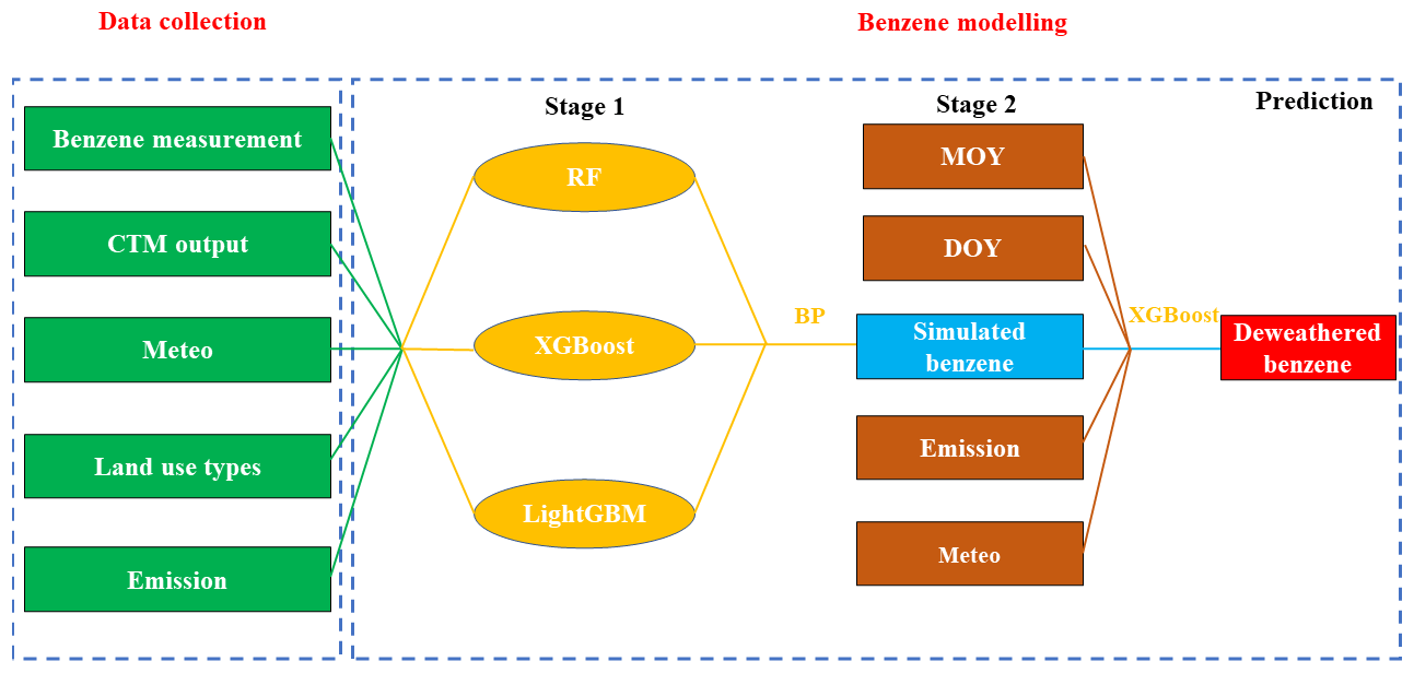
Figure 1 The workflow of global atmospheric benzene modelling. CTM output represents the simulated benzene concentration based on the GEOS-Chem model. Meteo denotes the meteorological parameters derived from GEOS-CF reanalysis. Emission represents the daily emissions of benzene. MOY and DOY are the month of year and day of year, respectively. Simulated benzene represents the predicted benzene concentrations based on the ensemble model. Deweathered benzene denotes the benzene concentration after removing meteorological effects.

Although all of these models showed good performance in predicting air pollutants, nearly all of the submodels still suffered from some weaknesses in their prediction accuracy. Hence, it was necessary to collocate these models using a back-propagation neutral network (BPNN) to further simulate daily ambient benzene concentrations at the global scale. As depicted in Fig. 1, three submodels including RF, XGBoost, and LightGBM were stacked through the BPNN model to simulate the daily atmospheric benzene levels at the global scale. Firstly, a 5-fold cross-validation method was utilized to train each submodel to determine the optimal hyperparameter. Then, the BPNN method was employed to further train the estimated concentrations of three submodels against the observations (Fig. 1). Lastly, the global ambient benzene concentrations were predicted on the basis of the ensemble model.

2.2.2 The meteorology-normalized benzene estimates

The ambient benzene concentration was influenced by both meteorological parameters and emissions. To isolate the contribution of emissions, the impacts of meteorological conditions should be removed. In our study, the XGBoost approach was utilized to eliminate the impacts of meteorological conditions. The simulated benzene concentration in each grid (0.25^∘) based on the method in Sect. 2.2.1 was treated as the dependent variable. The daily benzene emissions, meteorological factors, month of year (MOY), and day of year (DOY) in each grid were regarded as the explanatory variables. The raw dataset was randomly classified into a training dataset (90 % of input dataset) for developing the XGBoost model, and the remaining samples were regarded as the test dataset. After the development of the XGBoost model, the weather-normalized technique was employed to predict the ambient benzene concentration at a specific time point. The detailed deweathered algorithms were first introduced by Grange and Carslaw (2019). The meteorology-normalized benzene level served as the concentrations contributed by emissions alone. The differences in total and deweathered benzene concentrations were regarded as the concentration contributed by meteorology. In addition, the cross-validation (CV) R² value of the model used for the separation of meteorology and emissions should also be higher than 0.50; otherwise the model could be considered unreliable.

2.3 Health effect assessment

In our study, the carcinogenic and non-carcinogenic risks of ambient benzene were assessed based on the standard methodology of the United States Environmental Protection Agency (EPA). The carcinogenic and non-carcinogenic risks induced by benzene exposure were evaluated based on the lifetime carcinogenic risk (LCR) and hazard index (HI). The formulas for calculating benzene intake (BI), LCR, and HI are as follows (Table S1):

$$\begin{array}{}\text{(10)}& {\displaystyle }\text{BI}=(C\times \text{ET}\times \text{EF}\times \text{ED})/(\mathrm{365}\times \mathrm{24}\times \text{AT}),\text{(11)}& {\displaystyle }\text{HI}=\text{BI}/\text{RfC},\text{(12)}& {\displaystyle }\text{LCR}=\text{BI}\times \text{IUR},\end{array}$$

where C (µg m⁻³) denotes the concentration of the corresponding ambient benzene; ET is the exposure time; EF represents the annual exposure frequency (d a⁻¹); ED is the exposure duration (a); AT_nca and AT_ca denote the average exposure time for carcinogenic and non-carcinogenic risks (a), respectively; BI means the benzene intake; RfC represents the reference dose (µg m⁻³); and IUR is the inhalation risk (1/µg m⁻³). The non-carcinogenic risk of the ambient benzene is considered high when HI is above 1.0, whereas the health risk is not obvious when HI is below 1.0. The carcinogenic risk was regarded as definite risk when LCR was higher than $\mathrm{1}\times {\mathrm{10}}^{-\mathrm{4}}$, while it was treated as possible risk when this indicator was located between $\mathrm{1}\times {\mathrm{10}}^{-\mathrm{6}}$ and $\mathrm{1}\times {\mathrm{10}}^{-\mathrm{4}}$. The risk was treated as negligible when the indicator was lower than $\mathrm{1}\times {\mathrm{10}}^{-\mathrm{6}}$ (Dumanoglu et al., 2014; Li et al., 2017).

3 Results and discussion

3.1 The model fitting and validation

The ensemble model was utilized to estimate the ambient benzene concentrations at the global scale during 23 January–30 June in 2019 and 2020. The CV R² value of the ensemble model (R²=0.60) was significantly higher than that of RF (0.52), XGBoost (0.53), and LightGBM (0.55) (Fig. S3). Nevertheless, both the root-mean-square error (RMSE) (1.18 µg m⁻³) and the mean absolute error (MAE) (0.59 µg m⁻³) of the ensemble model were significantly lower than those of RF (RMSE and MAE: 1.41 and 0.72 µg m⁻³), XGBoost (RMSE and MAE: 1.37 and 0.70 µg m⁻³), and LightGBM (RMSE and MAE: 1.34 and 0.69 µg m⁻³). The higher R² value and the lower RMSE and MAE suggested the higher accuracy of the ensemble model in air quality simulation. In pioneering studies, Wolpert (1992) confirmed that the joint use of multiple statistical models could decrease the probability of overfitting and strengthen the predictive accuracy and transferability of final models. Besides, our previous studies also demonstrated that the stacking of various decision tree models could significantly outperform an individual model because each decision tree model could suffer from some weaknesses (Li et al., 2021). For instance, the dataset in the RF model appeared to be overfitted when much noise existed in the training data of regression problems (Breiman, 2001). Besides, the RF model might underestimate/overestimate the extreme values of ambient benzene (Xue et al., 2019), which could be neutralized by the XGBoost algorithm through the boosting method (Li et al., 2020). For XGBoost algorithm, excessive leaf nodes often showed low splitting gain, while the LightGBM model could make up for this defect (Nemeth et al., 2019). Overall, the combination of these decision tree models could overcome the weaknesses of the individual models and enhance the robustness of the final model.

Although 10-fold CV has verified that the modelling performance of the ensemble model was superior to that of the individual models, this method cannot examine the spatial transferability of this model. In our study, many regions (except India, Europe, and the United States) lacked monitoring sites for ambient benzene. Fortunately, the CTMs' output provided a strong proxy to predict the daily ambient benzene concentrations before and after the COVID-19 outbreak. In order to examine the spatial transferability of the ensemble model, cross-validation was performed. In each round, two-thirds of the benzene dataset in India, Europe, and the United States was applied to train the model, and the remaining third was utilized to examine the model (e.g. India + Europe for training and the United States for testing). After three rounds, all of the simulated benzene concentrations were compared with the corresponding observed values. As shown in Fig. S4, the out-of-bag R² value reached 0.58, which was slightly lower than the R² value (0.60) of the training model. In addition, the RMSE and MAE of the fitting equation for the out-of-bag data were 1.18 and 0.62, respectively. The results were in good agreement with those based on the CV database, indicating the ensemble model showed satisfactory spatial generalization.

The ensemble model can capture the spatiotemporal variation in ambient benzene during the COVID-19 lockdown period, while the impact of the COVID-19 lockdown cannot be quantified because the contribution of meteorological parameters cannot be removed based on this model alone. Therefore, it is proposed to employ the XGBoost algorithm to isolate the contribution of emission reduction to global atmospheric benzene. As depicted in Fig. S5, the CV R² value and slope of the fitting curve reached 0.65 and 0.62, respectively. The results suggest that the meteorology-normalized model was robust because the CV R² value was much higher than 0.50.

3.2 The impact of the COVID-19 lockdown on the global atmospheric benzene level

The ensemble model was developed to expand the ground-observed benzene measurement to the global scale and capture the global spatial variability in ambient benzene. As shown in Fig. S6, the global simulated (total) benzene concentration during 23 January–30 June in 2019 and 2020 ranged from 0.52 to 6.36 µg m⁻³, with an average value of 0.92±0.23 µg m⁻³. At the regional scale, the benzene concentration displayed significant spatial variability. The benzene concentration followed the order of India (1.44±0.14 µg m⁻³) > China (1.17±0.13 µg m⁻³) > Europe (1.02±0.08 µg m⁻³) > the United States (0.96±0.09 µg m⁻³) during 23 January–30 June in 2019 and 2020. Besides, the global simulated mean benzene level underwent a slight decrease from 0.93±0.06 in 2020 to 0.90±0.06 in 2019. However, the inter-annual variation in ambient benzene exhibited a remarkable spatial discrepancy at the global scale. As depicted in Fig. S7, the change ratio of the simulated (total) benzene level during the COVID-19 lockdown period (the difference in the benzene level before the COVID-19 lockdown and that during the COVID-19 lockdown period) in 2020 was in the order of India (−18.5 %) > Europe (−16.7 %) > China (−11.7 %) > the United States (−11.5 %). Compared with 2020, the change ratio of the benzene level during the same period in 2019 followed the order of India (−16.3 %) > Europe (−6.62 %) > the United States (−6.46 %) > China (−4.18 %). It should be noted that the simulated ambient benzene concentration had a higher decreasing ratio in 2020 compared with the same period in 2019 in nearly all of the major countries and regions around the world, which might be associated with the local COVID-19 lockdown measures in 2020.

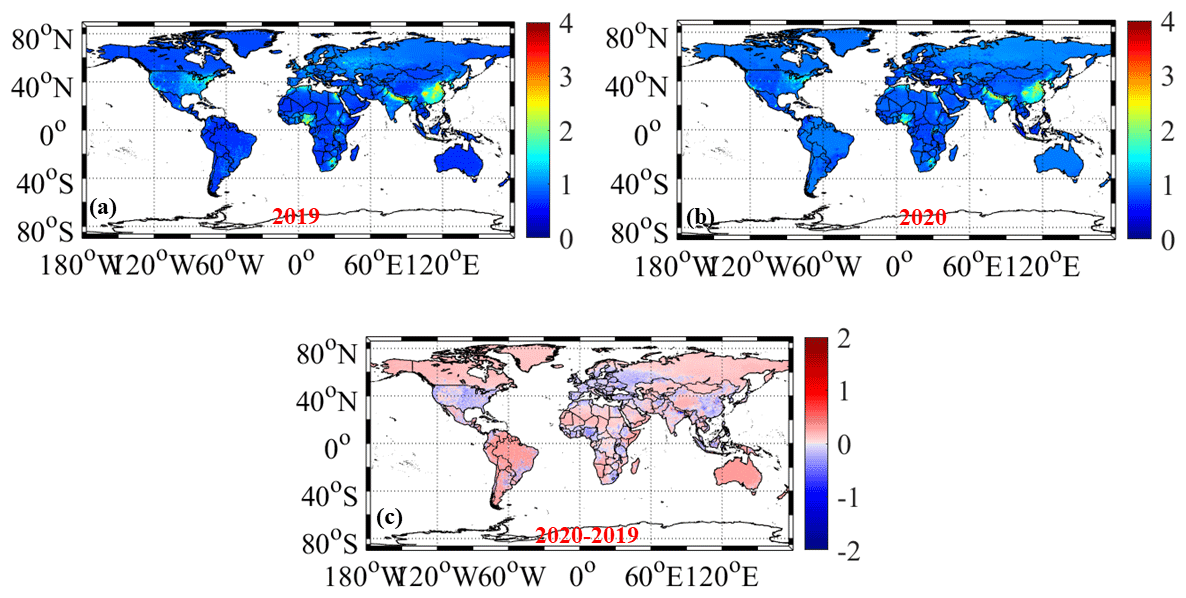
Figure 2 The global average deweathered benzene concentrations in 2019 (23 January–30 June) (a) and 2020 (23 January–30 June) (b). Panel (c) represents the difference in deweathered benzene concentrations in 2020 and 2019 (unit: µg m⁻³).

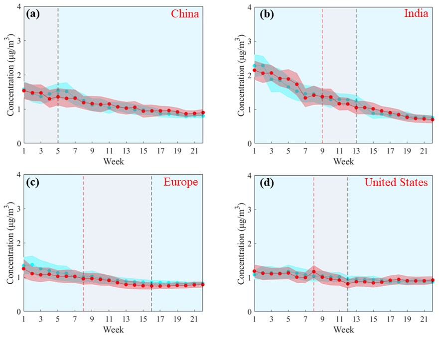
Figure 3 The weekly variations in atmospheric benzene concentrations (µg m⁻³) in some major regions around the world during 23 January–30 June. The red line and background denote mean values and standard deviation of deweathered weekly benzene concentrations in 2020. The cyan line and background denote mean values and standard deviation of deweathered weekly benzene levels in 2019. The dashed vertical red line indicates COVID-19 restriction dates, and the dashed vertical black line indicates the beginning of easing measures.

Table 1 The change ratio (%) of deweathered (P_dew) and detrended (P^∗) benzene concentrations in major regions around the world.

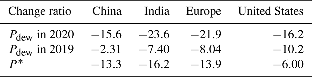
Due to the interference of meteorological conditions, we cannot quantify the direct impact of the COVID-19 lockdown on ambient benzene based on the comparison of simulated (total) benzene levels. Thus, the meteorology-normalized method was employed to decouple the separated contributions of emission reduction and meteorology to ambient benzene. In our study, both the change ratio and the detrended change ratio were applied to evaluate the impact of the COVID-19 lockdown on the global ambient benzene level. The change ratio represents the variation in the ambient benzene level during the lockdown period in 2020 compared with the pre-lockdown period in 2020. However, the detrended change ratio reflects the difference in the change ratio in 2020 and the change ratio during the same period in 2019, which could avoid the inter-annual system error and contingency of a single year. As summarized in Figs. 2 and 3, the change ratio of the deweathered benzene concentration from the pre-lockdown to lockdown period in 2020 was in the order of India (−23.6 %) > Europe (−21.9 %) > the United States (−16.2 %) > China (−15.6 %). Meanwhile, the change ratio of the deweathered benzene concentration during the same time in 2019 followed the order of Europe (−10.2 %) > the United States (−8.04 %) > India (−7.40 %) > China (−2.31 %). The large gap in the change ratio of the deweathered benzene level between 2019 and 2020 confirmed that the drastic and consequential quarantine measures significantly decreased the ambient benzene concentrations in nearly all of the regions with lockdown measures. Among all of the major countries and regions, India experienced the most dramatic benzene decrease during 24 March–24 April 2020 (−23.6 %) compared with the same period in 2019 (−7.4 %). During this period, the prohibition of industrial activities and mass transportation was proposed to curb the spread of the COVID-19 pandemic, leading to a tremendous reduction in anthropogenic benzene emissions (Pathakoti et al., 2021; Zhang et al., 2021). Sahu et al. (2022) revealed that the substantial increase in OH radicals during the COVID-19 period also facilitated ambient benzene removal due to the photooxidation reaction. The decreasing ratio of the deweathered benzene level in India was close to that of PM_2.5 (−26 %), while it is was markedly lower than that of NO₂ (−50 %) (Zhang et al., 2021). Although both Europe and the United States also performed stringent lockdown restrictions in some regions such as Italy, Spain, and California (Guevara et al., 2021a; Keller et al., 2021a), the detrended change (P^∗: change ratio in 2020 − change ratio in 2019) for deweathered benzene in Europe ($P^{\ast }=-\mathrm{13.9}$ %) and the United States ($P^{\ast }=-\mathrm{6}$ %) between 2020 and 2019 was still lower than that of India ($P^{\ast }=-\mathrm{16.2}$ %) (Table 1). It was assumed that the absolute concentrations of ambient benzene in Europe and the United States were much lower than that in India. It should be noted that China displayed a relatively gently decreasing ratio (−15.6 %) after the COVID-19 outbreak, which was even lower than the ratio in the United States. As the first epidemic epicentre country, the Chinese government imposed a rapid lockdown measure in Wuhan and other cities across China in an effort to prevent the spread of the COVID-19 pandemic (Wu et al., 2020). These restrictions interrupted a wide array of economic activities and reduced primary air pollutant emissions and thus resulted in remarkable decreases in deweathered NO₂ (−43.6 %) and PM_2.5 (−22 %) (Dai et al., 2021). The gently decreasing ratio of ambient benzene compared with other pollutants might be linked with the source apportionment of atmospheric benzene. It was well known that industrial sources (e.g. the chemical industry and solvent use) comprised the major emission sector of benzene (Li et al., 2019). Although the contribution from solvent use exhibited substantial decreases in some cities (Qi et al., 2021; Wang et al., 2021), the chemical industry was not entirely interrupted even during the COVID-19 lockdown period (Dai et al., 2021). B. Zheng et al. (2021) also demonstrated that reduction in NMVOC emissions from the industrial sector was much less than for other pollutants.

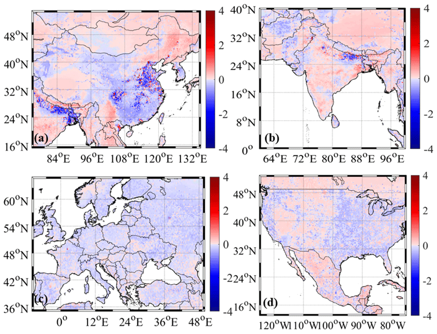
Figure 4 The concentration difference for deweathered benzene between the COVID-19 period in 2020 and the same period in 2019 in (a) East Asia, (b) South Asia, (c) Europe, and (d) North America (difference = deweathered benzene concentration in 2020 − deweathered benzene concentration in 2019) (unit: µg m⁻³).

Although the deweathered benzene concentrations in nearly all of the major countries underwent obvious decreases during the COVID-19 lockdown period, the change ratios of deweathered benzene in different regions of these countries still showed large spatial variability. In China, most of the cities in eastern China such as Beijing (−30.6 %), Shanghai (−6.25 %), and Wuhan (−45.3 %) experienced dramatic decreases in deweathered benzene levels (Fig. S8), which was mainly contributed by the simultaneous emission reduction of the industrial and transportation sectors. Besides, enhanced atmospheric oxidation capacity could have accelerated the benzene removal due to the unbalanced decreases in VOC and NO_x emissions (Jensen et al., 2021). However, the deweathered benzene concentrations in northeastern China and Yunnan Province even exhibited slight increases after the COVID-19 outbreak (Fig. 4). Dai et al. (2021) also found that the deweathered PM_2.5 concentration in Kunming increased ∼20 % after the COVID-19 outbreak. At first, the contribution of residential combustion sources (62.1 %) to atmospheric benzene in Yunnan Province was higher than that of other sectors (Guevara et al., 2021b; Kuenen et al., 2022). Moreover, the increase in domestic emissions due to home quarantine regulations further increased the ambient benzene concentration (10 %) in this province, which has been demonstrated by the updated emission inventory in 2020 (Doumbia et al., 2021). The slight increases in deweathered benzene levels in northeastern China after the COVID-19 outbreak could be linked with earlier work resumption (https://baijiahao.baidu.com/s?id=1658138056285012986&wfr=spider&for=pc, last access: 15 December 2022). Based on the simulation result, the deweathered ambient benzene level in northeastern China rebounded sharply after the third week and then returned back to normal in late February. In India, the decreasing ratios of deweathered benzene in Delhi, Mumbai, Kolkata, Bengaluru, Hyderabad, Chennai, Ahmedabad, and Lucknow reached 21.6 %, 20.9 %, 73.7 %, 26.9 %, 38.0 %, 33.7 %, 25.1 %, and 33.3 %, respectively, during the COVID-19 lockdown period (Fig. S9). Among all of the major cities in India, the ambient benzene level in Kolkata underwent the most drastic decrease. It was assumed that Kolkata is a dusty city and filled with vehicle emissions. Fortunately, the city experienced a complete stop of vehicle movement and of burning of biomass and dust particles from construction works, which had been important sources for ambient benzene (Bera et al., 2021; Kumar and Singh, 2003). In Europe, the deweathered benzene levels in nearly all of the cities displayed marked decreases because most European countries imposed lockdowns to combat the spread of the COVID-19 pandemic (Guevara et al., 2021a). For example, private cars and heavy goods vehicles (HGVs) on the road in London reduced by 80 % and 30 %–40 %, respectively (Shi et al., 2021). The drastic decrease in transportation emissions triggered the P^∗ value in London between 2020 and 2019 reaching −43.6 %. In the United States, the decreasing ratios of deweathered benzene levels in the cities of the eastern United States and California were generally higher than those in the central United States, which was in good agreement with the spatial variability in the PM_2.5 decrease (Hammer et al., 2021). It was closely associated with the length of the lockdown period (https://en.wikipedia.org/wiki/COVID-19_lockdowns, last access: 14 January 2023).

In addition, ambient benzene levels were also strongly affected by meteorological conditions that alter photochemical production, advection, and depositional loss. Hence, we examined how meteorological parameters influenced the temporal variability in ambient benzene during the COVID-19 lockdown period. In 2020, most of the major countries and regions including China (3.9 %), Europe (5.2 %), and the United States (4.7 %) experienced slightly unfavourable meteorological conditions, which is in good agreement with the impact of meteorological conditions on ambient NO₂ concentrations (Shi et al., 2021). Among all the meteorological parameters, air temperature was the most important factor for ambient benzene in nearly all of the regions around the world during the study period. Compared with 2019, the air temperatures in China, India, Europe, and the United States increased by 0.4, 0.9, 0.4, and 0.2 ^∘C during the same period in 2020, respectively. Jia and Xu (2014) demonstrated that the increased air temperature generally suppressed benzene photooxidation and secondary organic aerosol (SOA) formation. Thus, the increased air temperature was not beneficial to the further reduction in ambient benzene. Apart from air temperature, some other factors such as RH, rainfall amount, and wind speed might have affected the ambient benzene level. For instance, the increased RH could have been favourable to benzene oxidation and the higher rainfall amount could have promoted benzene removal. However, in the machine-learning model, the importance values of these variables were much lower than that of air temperature. Overall, the results suggest that the unfavourable meteorological conditions (air temperature) weakened the health benefits of reduced ambient benzene due to drastic lockdown measures around the world.

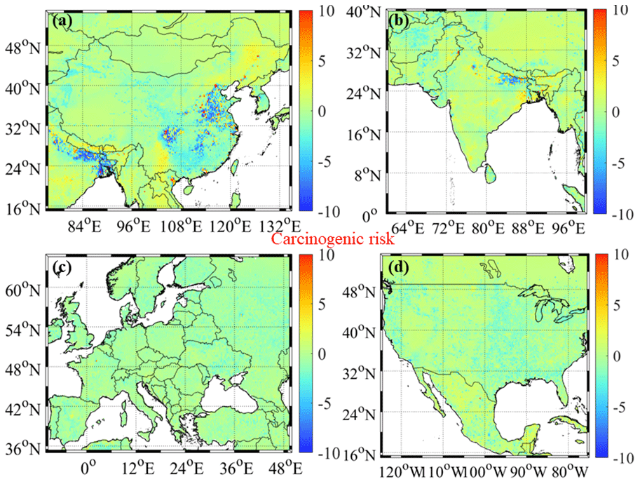
Figure 5 The carcinogenic risk differences (unit: 10⁻⁷) for atmospheric benzene between the COVID-19 period in 2020 and the same period in 2019 in (a) East Asia, (b) South Asia, (c) Europe, and (d) North America (difference = benzene concentration in 2020 − benzene concentration in 2019).

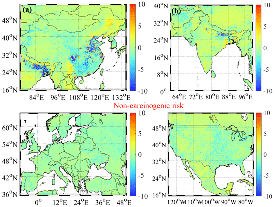
Figure 6 The non-carcinogenic risk differences (unit: 10⁻³) for atmospheric benzene between the COVID-19 period in 2020 and the same period in 2019 in (a) East Asia, (b) South Asia, (c) Europe, and (d) North America (difference = benzene concentration in 2020 − benzene concentration in 2019).

3.3 The effect of the COVID-19 lockdown on global health risks

The global average LCR during 23 January–30 June in 2019 and 2020 was $\mathrm{4.89}\times {\mathrm{10}}^{-\mathrm{7}}$ and $\mathrm{4.51}\times {\mathrm{10}}^{-\mathrm{7}}$, respectively, after removing the contributions of meteorological conditions (Fig. S10). Although the COVID-19 lockdown decreased the LCR value slightly, both of the LCR values during the two periods were lower than the threshold level of 10⁻⁶, suggesting that dwellings in most regions could avoid carcinogenic risk through inhalation exposure to benzene (Li et al., 2017). However, the LCR values showed significant spatial difference in different regions. For instance, northern China often suffered from relatively high benzene pollution, and the LCR value in this region decreased from $\mathrm{1.03}\times {\mathrm{10}}^{-\mathrm{6}}$ (possible risk) during the study period in 2019 (the same period to 2020) to $\mathrm{7.37}\times {\mathrm{10}}^{-\mathrm{7}}$ during the COVID-19 lockdown period. The result verified that the stringent emission control measures significantly decreased the health risk due to benzene exposure. The LCR value across India only decreased from $\mathrm{6.55}\times {\mathrm{10}}^{-\mathrm{7}}$ to $\mathrm{6.42}\times {\mathrm{10}}^{-\mathrm{7}}$ during the study period, whereas the value in the northern part of India, including for example Bihar, decreased from $\mathrm{1.14}\times {\mathrm{10}}^{-\mathrm{6}}$ to $\mathrm{1.09}\times {\mathrm{10}}^{-\mathrm{6}}$ due to the impact of the COVID-19 lockdown (Fig. 5). As the most populous state of India, Bihar had more than 124 million people at the time (http://kolkata.china-consulate.org/chn/lqgk/t1331638.htm, last access: 31 January 2023). The results suggest that the COVID-19 lockdown certainly obtained remarkable short-term health benefits through decreasing ambient benzene exposure. The LCR values in Europe and the United States decreased from $\mathrm{4.99}\times {\mathrm{10}}^{-\mathrm{7}}$ and $\mathrm{4.77}\times {\mathrm{10}}^{-\mathrm{7}}$ to $\mathrm{4.57}\times {\mathrm{10}}^{-\mathrm{7}}$ and $\mathrm{4.63}\times {\mathrm{10}}^{-\mathrm{7}}$, respectively. Compared with China and India, Europe and the United States faced relatively low carcinogenic risk of benzene exposure even before the COVID-19 lockdown. Although the COVID-19 lockdown further decreased the LCR values in these regions, the overall carcinogenic risk was negligible.

Additionally, the non-carcinogenic risk around the world during the period was also assessed based on HI. The average HI of ambient benzene exposure in China, India, Europe, and the United States reduced from $\mathrm{8.92}\times {\mathrm{10}}^{-\mathrm{3}}$, $\mathrm{7.45}\times {\mathrm{10}}^{-\mathrm{3}}$, $\mathrm{6.32}\times {\mathrm{10}}^{-\mathrm{3}}$, and $\mathrm{5.76}\times {\mathrm{10}}^{-\mathrm{3}}$ in 2019 to $\mathrm{8.53}\times {\mathrm{10}}^{-\mathrm{3}}$, $\mathrm{7.13}\times {\mathrm{10}}^{-\mathrm{3}}$, $\mathrm{5.81}\times {\mathrm{10}}^{-\mathrm{3}}$, and $\mathrm{5.59}\times {\mathrm{10}}^{-\mathrm{3}}$, respectively, during the COVID-19 lockdown period in 2020 (Fig. 6). Although the HI value in some regions including Bihar ($\mathrm{1.52}\times {\mathrm{10}}^{-\mathrm{2}}$ to $\mathrm{1.41}\times {\mathrm{10}}^{-\mathrm{2}}$) and Uttar Pradesh ($\mathrm{1.04}\times {\mathrm{10}}^{-\mathrm{2}}$ to $\mathrm{1.03}\times {\mathrm{10}}^{-\mathrm{2}}$) in India and Beijing–Tianjin–Hebei (BTH) ($\mathrm{1.25}\times {\mathrm{10}}^{-\mathrm{2}}$ to $\mathrm{1.14}\times {\mathrm{10}}^{-\mathrm{2}}$) in China still experienced decreases during the COVID-19 lockdown period, the HI values in these regions were still significantly lower than the risk threshold (HI = 1). Therefore, the impact of the COVID-19 lockdown on the non-carcinogenic risk of benzene exposure was insignificant.

4 Conclusions and limitations

The drastic lockdown measures largely reduced the air pollutant emissions. The meteorology-normalized ambient benzene concentrations in China (−15.6 %), India (−23.6 %), Europe (−21.9 %), and the United States (−16.2 %) experienced dramatic decreases after the COVID-19 outbreak. Furthermore, the decreasing ratios in these major regions during the COVID-19 lockdown period were much higher than in the same period in 2019, indicating the aggressive emission control measures efficiently decreased ambient benzene concentrations. Emission reductions from industrial activities and transportation were major drivers of the decrease in the ambient benzene level during the lockdown period, while the relatively stable solvent use emissions could have restricted a further decrease in benzene pollution. Besides, the slight increase in domestic emissions during this period might be an important reason for the benzene increase in some regions (e.g. Yunnan Province). There is also an urgent need to control the household combustion and solvent use emissions in addition to the emissions from the industrial and transportation sectors.

Besides, substantial decreases in atmospheric benzene levels could have sufficient health benefits. Dramatic decreases in benzene emissions in Europe and the United States could not have brought about effective health benefits because the ambient benzene levels in both of these regions during the business-as-usual scenario were already significantly lower than the risk threshold. However, the benzene decreases in the North China Plain (NCP), China, and Bihar, India, could have had abundant health benefits because these regions often suffered from severe atmospheric benzene pollution during the business-as-usual scenario. Thus, more targeted abatement measures are needed to reduce the benzene emissions in these areas. For instance, stricter industrial and vehicle emission standards for VOC control should be implemented in China and India. Moreover, some measures including limiting the number of coal-fired power plants, adding environmentally friendly cars and clean fuels for vehicles and vessels, and strengthening the labelling system for vehicles in use should be pursued.

It should be noted that our study still suffered from some limitations. First of all, the monitoring sites were not evenly distributed around the world, and thus the simulation results might show higher uncertainty in the regions lacking monitoring sites. Besides, the GEOS-Chem model still suffered from some uncertainties due to an imperfect chemical mechanism and inaccurate emission inventory. In future work, the model should be further improved.