Estimating hub-height wind speed based on a machine learning algorithm: implications for wind energy assessment

Accurate estimation of wind speed at wind turbine hub height is of significance for wind energy assessment and exploitation. Nevertheless, the traditional power law method (PLM) generally estimates the hub-height wind speed by assuming a constant exponent between surface and hub-height wind speed. This inevitably leads to significant uncertainties in estimating the wind speed profile especially under unstable conditions. To minimize the uncertainties, we here use a machine learning algorithm known as random forest (RF) to estimate the wind speed at hub heights such as at 120 m (WS₁₂₀), 160 m (WS₁₆₀), and 200 m (WS₂₀₀). These heights go beyond the traditional wind mast limit of 100–120 m. The radar wind profiler and surface synoptic observations at the Qingdao station from May 2018 to August 2020 are used as key inputs to develop the RF model. A deep analysis of the RF model construction has been performed to ensure its applicability. Afterwards, the RF model and the PLM model are used to retrieve WS₁₂₀, WS₁₆₀, and WS₂₀₀. The comparison analyses from both RF and PLM models are performed against radiosonde wind measurements. At 120 m, the RF model shows a relatively higher correlation coefficient R of 0.93 and a smaller RMSE of 1.09 m s⁻¹, compared with the R of 0.89 and RMSE of 1.50 m s⁻¹ for the PLM. Notably, the metrics used to determine the performance of the model decline sharply with height for the PLM model, as opposed to the stable variation for the RF model. This suggests the RF model exhibits advantages over the traditional PLM model. This is because the RF model considers well the factors such as surface friction and heat transfer. The diurnal and seasonal variations in WS₁₂₀, WS₁₆₀, and WS₂₀₀ from RF are then analyzed. The hourly WS₁₂₀ is large during daytime from 09:00 to 16:00 local solar time (LST) and reach a peak at 14:00 LST. The seasonal WS₁₂₀ is large in spring and winter and is low in summer and autumn. The diurnal and seasonal variations in WS₁₆₀ and WS₂₀₀ are similar to those of WS₁₂₀. Finally, we investigated the absolute percentage error (APE) of wind power density between the RF and PLM models at different heights. In the vertical direction, the APE is gradually increased as the height increases. Overall, the PLM algorithm has some limitations in estimating wind speed at hub height. The RF model, which combines more observations or auxiliary data, is more suitable for the hub-height wind speed estimation. These findings obtained here have great implications for development and utilization in the wind energy industry in the future.

1 Introduction

With the rapid economic development of the world, the massive consumption of fossil fuels produces an increasing emission of carbon dioxide, sulfur dioxide, and other pollutants (Yuan, 2016; Magazzino et al., 2021). To tackle this problem, it is increasingly becoming imperative to develop renewable clean energy (Hong et al., 2012; Luo et al., 2022). Among the myriad renewable energy resources, wind energy has gained more and more favor because of its abundant availability, good sustainability, and high cost-effectiveness (Li et al., 2018; Leung et al., 2012). As one of the largest energy consuming countries in the world, China is currently facing an increasingly serious energy and climate situation (Khatib et al., 2012). The Chinese government proposes to peak its carbon dioxide emissions before 2030 and achieve carbon neutrality before 2060 (Shi et al., 2023; Su et al., 2022a, b). With the stimulus of policies and the favor of investors, the wind power industry in China is flourishing. Therefore, the scientific assessment of wind energy resources in China is of great importance for the healthy development of the wind energy industry in the decades to come.

Characterizing the wind speed at wind turbine hub height is key for wind energy assessment (Yu and Vautard, 2022). The wind turbine is usually installed at the top of the wind mast with a height of 100–120 m above ground level (a.g.l.), which roughly corresponds to the surface layer (Veers et al., 2019). The wind speed data that have been widely used for wind energy assessment are mainly obtained from wind mast, Doppler lidar, or reanalysis data (Debnath et al., 2021; Lolli et al., 2011; Lolli, 2021). The 10 m wind data measured by ground meteorological stations can be used for wind energy assessment (Oh et al., 2012; Liu et al., 2019). The wind tower or mast can also provide wind speed observation data below 100 m a.g.l. (Durisic et al., 2012; J. Liu et al., 2018). Moreover, the reanalysis data, such as the fifth generation European Centre for Medium-Range Weather Forecasts atmospheric reanalysis system (ERA5), can provide the hourly wind speed at a height of 10 or 100 m a.g.l. for wind energy assessment (Laurila et al., 2021; Gualtieri, 2021). However, the wind turbines are increasing in height and rotor diameter with the development of technology, which go beyond the surface layer and enter the Ekman layer. Such as for some offshore wind power plants, the blade tips of the largest wind turbines can reach heights of 250 m a.g.l. (Gaertner et al., 2020). In addition, increasing wind turbine hub height reduces the impact of surface friction, enabling wind turbines to operate in high-quality wind resource environments (Veers et al., 2019). Therefore, the wind profile is important for the selection of wind turbine hub height and the assessment of wind energy.

It is widely recognized that the wind profile is mainly obtained by empirical formulae (Li et al., 2018), such as the power law method (PLM). The PLM generally assumes that the wind speed below 150 m in the planetary boundary layer (PBL) varies exponentially with height (Hellman et al., 1914). This means that the wind speed at the wind turbine hub height can be calculated from the surface wind speed based on a constant power law exponent (α). However, the surface-layer wind profile is mainly controlled by the surface roughness, friction velocity, and the atmospheric stability (Gryning et al., 2007). The surface layer is where obstructions such as trees, buildings, hills, and valleys cause turbulence and reduce the wind speed (Coleman et al., 2021; Solanki et al., 2022). Due to the influence of an inhomogeneous underlying surface and ubiquitous atmospheric turbulence, wind speed varies constantly and greatly in the vertical (Tieleman, 1992). Especially above the surface layer, factors such as the Coriolis force, baroclinity, and wind shear increase the complexity of the wind profile (Brümmer, 1991). As a result, the α has spatiotemporal variability and depends on a variety of factors, such as terrain, time, and height (Li et al., 2018). Therefore, the assumption of a constant α poses great challenges and uncertainties to wind energy assessment. Some studies use more complex models to improve the PLM, such as the perturbation theory (Sen et al., 2012) and the bivariate wind speed–wind shear model (Jung et al., 2017). These studies confirm that there is a complex nonlinear relationship between surface observations and wind speed at the wind turbine hub height. Therefore, one of the greatest challenges is to develop an accurate method to describe the nonlinear transfer from surface observations to wind speed at wind turbine hub height.

With the development of machine learning (ML) technology, ML algorithms have been widely used in the field of wind speed and wind power prediction (Magazzino et al., 2021). Chi et al. (2015) compared two wind speed-forecasting mechanisms in China based on linear regression and support vector machine algorithms. They find that ML algorithms have better accuracy in solving the nonlinear problem. Lahouar and Slama (2017) use several meteorological factors to forecast wind power based on a random forest (RF) model. The results indicate that, compared with physical and statistical approaches, the ML model can achieve better accuracy when coping with problems that cannot be analytically defined. Therefore, it is worth trying to use ML algorithms to retrieve the wind speed at wind turbine hub height from available observations.

Given the abovementioned problems, we attempt to use a ML algorithm known as RF to retrieve wind speed at wind turbine hub height from a radar wind profiler (RWP) and surface synoptic observations. An RF model has been trained based on the surface in situ wind speed, upper-height RWP wind speed, and corresponding surface meteorological data from May 2018 to August 2020. The performances of the classical PLM model and the RF model are then compared. Next, the wind speeds from the RF model are used to evaluate the wind power. The results of our study can provide useful information for the development of the wind energy industry in coastal China. The observational data are introduced in Sect. 2. The RF model construction and wind energy evaluation method are displayed in Sect. 3. Section 4 discusses the accuracy of the RF model and the variation in wind energy resources. A summary of results is presented in Sect. 5.

2 Materials and data

2.1 RWP data

The RWP is a ground-based remote sensing device that is used to measure the atmospheric wind profiles from the surface to 5–8 km a.g.l. (B. Liu et al., 2019; Guo et al., 2021a). It has high and low detection modes in the vertical direction, and their corresponding vertical resolutions are 120 and 60 m, respectively (Liu et al., 2020; Chen et al., 2023). Nevertheless, the wind profiles near the ground surface, especially those below 300 m a.g.l., are usually highly uncertain due to the influence of the ground and intermittent clutter (May and Strauch, 1998; Allabakash et al., 2019). Therefore, there exists a large data gap between ground surface and the lowest measurement height provided by the RWP. Here, the RWP data are obtained at Qingdao (36.33^∘ N, 120.23^∘ E), which is a typical coastal synoptic weather station. The spatial distribution and surface type of this station are shown in Fig. 1. Geographically, Qingdao station is located on the south of Shandong Peninsula and lies to the west of the Yellow Sea. To be more specific, this station is set up in a suburb surrounded by cropland. The altitude of this station is 12 m above mean sea level. The hourly wind speed (WS₃₀₀) and direction (WD₃₀₀) data at 300 m a.g.l. are obtained from 1 May 2018 to 31 August 2020. The original RWP data at 6 min intervals have not been released temporarily but can be requested upon reasonable demand by contacting Jianping Guo (email: jpguocams@gmail.com).

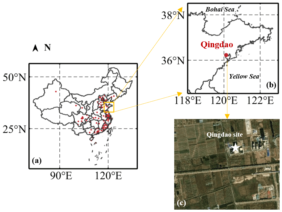
Figure 1 (a, b) Geographical distribution and (c) surface type of the radar wind profiler station at Qingdao. The surface type photo is provided by Google Earth (© Google Maps).

2.2 Anemometer

The wind cup anemometer can measure the instantaneous wind speed and is installed at 10 m a.g.l. (Mo et al., 2015). The sensing part of the wind cup anemometer is composed of three or four conical or hemispherical empty cups. It can provide surface wind data with an error of less than 10 % (Zhang et al., 2020). This device is also installed at Qingdao station. Here, the 10 m wind speed (WS₁₀) and direction (WD₁₀) data are also obtained from 1 May 2018 to 31 August 2020. The WS₁₀ data are processed into hourly average values to match the RWP data.

2.3 Radiosonde data

The radiosonde (RS) provides the vertical profiles of wind speed and wind direction at 5–8 m intervals (Guo et al., 2020). The accuracy of RS wind speed is within 0.1 m s⁻¹ in the PBL (Guo et al., 2021b). One noteworthy drawback is that the operational RS can provide observations of wind profiles only twice per day: 08:00 and 20:00 local solar time (LST). The Qingdao station is equipped with both an RS and an RWP. The RS data also collect from 1 May 2018 to 31 August 2020.

2.4 ERA5 data

The ERA5 is the reanalysis data combining model data and observations, which provides global hourly estimates of atmospheric variables (Hoffmann et al., 2019). The horizontal resolution can reach 0.25×0.25^∘, and there are 137 vertical levels in the vertical direction. “ERA5 hourly data on single levels from 1959 to present” is a dataset of ERA5 which can provide a series of surface parameters such as temperature, humidity, pressure, and radiation (Hersbach et al., 2020). Here, nine parameters have been collected, including Charnock coefficient (Char), forecast surface roughness (FSR), friction velocity (FV), dew point (DP), temperature (Temp), pressure (Pres), net solar radiation (R_n), latent heat flux (LHF), and sensible heat flux (SHF). Char, FSR, and FV are related to surface roughness and can evaluate the influence of different surface types on the wind speed in the surface layer. DP, Temp, and Pres are the meteorological parameters associated with wind speed. R_n, LHF, and SHF indicate the solar radiation level, which is directly related to the generation of wind. According to the longitude and latitude information of the Qingdao station, the grid where the RWP station is located is selected, and those parameters in the corresponding grid are obtained accordingly. These data are obtained from 1 May 2018 to 31 August 2020.

3 Methods

The schematic diagram of surface-layer wind profile observations is shown in Fig. 2. The wind mast or tower can provide wind speed data below 100 m a.g.l. (Durisic et al., 2012; J. Liu et al., 2018). The RWP can measure the wind profiles from 300 m to a height of 5–8 km a.g.l. (B. Liu et al., 2019). It leads to a gap (100 to 300 m) in the observations of the wind profile. At present, the PLM is most often applied to extrapolate the surface wind speed to the wind turbine hub height, such as wind speed at 120 m (WS₁₂₀), 160 m (WS₁₆₀), and 200 m (WS₂₀₀) a.g.l.

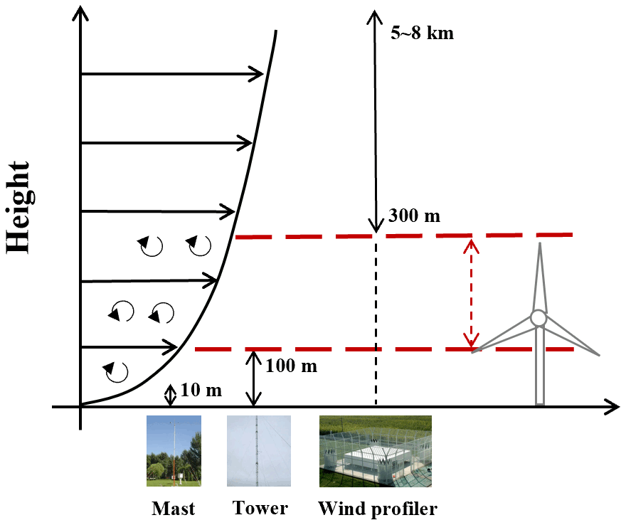
Figure 2 The schematic diagram of surface-layer wind profile observations. The photos are provided by Baidu (© Baidu).

3.1 Power law method

The PLM was proposed by Hellman et al. (1914). It assumes that the wind speed below 150 m in the PBL varies exponentially with height. As a result, the wind speed at wind turbine hub height is typically estimated using the following formula (Abbes et al., 2012):

$$\begin{array}{}\text{(1)}& v_{\mathrm{2}}=v_{\mathrm{1}}\times {\left({\displaystyle \frac{h_{\mathrm{2}}}{h_{\mathrm{1}}}}\right)}^{\mathit{\alpha }},\end{array}$$

where v₁ and v₂ are the wind speed at height h₁ and h₂, respectively. The α is the power law exponent, which varies with time, altitude, and location (Durisic et al., 2012). In engineering applications, the value of α is determined by the terrain type and generally is estimated to range from 0.1 to 0.4 (Li et al., 2018). Here, the general value of α for coastal topography is set to 0.15 based on former studies (Patel et al., 2005; Banuelos-Ruedas et al., 2010). However, Jung et al. (2021) pointed out that the error in the wind power density estimation over China can reach 30 % based on a constant α value. Therefore, we attempt to use an ML algorithm to obtain WS₁₂₀, WS₁₆₀, and WS₂₀₀.

3.2 RF algorithm

RF is an ensemble ML method which has been widely used in regressive calculations (Breiman, 2001). It is a method to integrate many decision trees into forests and predict the result. A schematic diagram of RF is shown in Fig. S1. RF is composed of many decision trees, and each decision tree is irrelevant. The performance of RF is determined by the aggregation of the results of all the trees (Ma et al., 2021). For the RF model, the number of trees (N) is an important parameter to achieve the optimal performance of the model. Further detailed information can be found in Breiman (2001).

3.2.1 Inputs for RF

In the construction of the RF model, it is necessary to obtain the relevant variables that may affect the surface wind profile according to the physical mechanism and previous research. At present, the PLM is often used to calculate the wind speed at hub height. It confirms that the wind speed at hub height is related to the wind speed at other heights (Durisic et al., 2012; Li et al., 2018). Therefore, WS₁₀, WD₁₀, WS₃₀₀, and WD₃₀₀ are selected as inputs. The surface wind profile also depends on the surface roughness, FV, and the atmospheric stability (Gryning et al., 2007) so that FSR, FV, and Char are also regarded as inputs. The higher FSR causes a slower wind speed in the surface layer. The FV is a theoretical wind speed at the Earth's surface which is used to calculate the way wind changes with height near the surface (Stull, 1988). Moreover, considering that the generation of wind is closely associated with uneven heating of the Earth's surface by solar radiation (Solanki et al., 2022), the R_n, LHF, and SHF are also selected as input variables. Additionally, some studies use atmospheric temperature and pressure as input to improve the accuracy of wind speed predictions (Chi et al., 2015). Here, we also regard DP, Temp, and Pres as the input variables. The reference value, also included as input in the RF model, is WS₁₂₀, WS₁₆₀, and WS₂₀₀ measured from RS. These values are listed in Table S1.

3.2.2 Feature selection

To estimate WS₁₂₀, WS₁₆₀, and WS₂₀₀, we need to build an RF model for 120 m (RF₁₂₀), 160 m (RF₁₆₀), and 200 m (RF₂₀₀), respectively. For each model, it is necessary to select the main features from the inputs to avoid data redundancy and reduce the complexity of the model (Ma et al., 2021). Following the research of De Arruda Moreira et al. (2022), the inputs which cannot cause a 2 % reduction in correlation coefficient are regarded as irrelevant features and are removed. Figure 3 shows the importance analysis of inputs for three RF models. The relevant features are marked by red bars. The irrelevant features are marked by blue bars, which are not regarded as final inputs in three RF models. For three RF models, the relevant features are WS₁₀, FV, Char, SHF, and WS₃₀₀. It indicates that the factors such as surface friction, heat transfer, and upper-height wind speed constraints are considered in the construction of RF models. In addition, it is surprising that FSR has such low importance in three RF model constructions. FSR is a measure of surface resistance, which directly affects the near-surface wind speed (Gryning et al., 2007). At a land station, FSR is derived from the vegetation type (Li et al., 2021). The surface type of Qingdao station is cropland. Li et al. (2021) confirms that the FSR for cropland is most likely up to 0.3 m. In training data, the FSR from ERA5 also approximates a constant value (0.3 m). Since the constant variable has no meaning for RF model construction, the RF model divides FSR into irrelevant variables. Therefore, the final inputs for three RF models are WS₁₀, FV, Char, SHF, and WS₃₀₀.

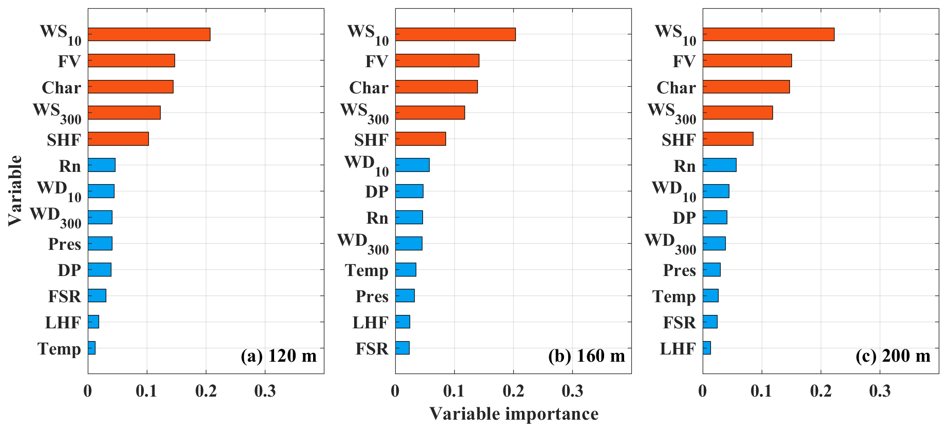
Figure 3 Importance analysis of inputs for the RF model at (a) 120 m, (b) 160 m, and (c) 200 m.

3.2.3 Tuning parameter

The RF algorithm requires the N to be setup in order to avoid overfitting in the training dataset (Ma et al., 2021). Here, we use the RF algorithm for regression in MATLAB R2020b. The code and usage of RF are found at the MATLAB help center (https://ww2.mathworks.cn/help/stats/treebagger.html, last access: 15 November 2022). The specific tuning parameter process of the RF model is presented as follows: the N value varies from 1–500 with an interval of 10. Correlation coefficient (R) and root mean square error (RMSE) are used to evaluate the accuracy of the model. We need to set an appropriate N value to maximize R and minimize RMSE. Figure S2 shows the tuning parameter process for the N of three RF models. For RF₁₂₀, it was found that the R increased when the N value increased, while the R is almost unchanged when the N value is greater than 100. When N equals 200, R reaches the maximum value (0.82) and RMSE reaches the minimum value (1.68 m s⁻¹). Therefore, the N value is set to 200 for RF₁₂₀. Moreover, according to the same tuning parameter process, the N values are set to 300 and 150 for RF₁₆₀ and RF₂₀₀, respectively. After determining the final inputs and N values, the three RF models were trained and tested. At Qingdao station, a total of 746 sample data are obtained after data matching. We use the fivefold crossover to train the RF models. The test results are discussed in Sect. 4.1.

3.2.4 Sensitivity analysis

The accuracy and generalization of the RF model depend on training and testing samples (Ma et al., 2021). However, the training and testing samples are obtained at 08:00 and 20:00 LST. It needs to be discussed whether the RF model also applies to other times. This depends on whether the RF model has enough generalization for the training samples and whether the inputs at other times have appeared in the training samples. Figures S3–S5 show the differences between estimated wind speed and observed wind speed of the three RF models, which are a function of the inputs. For the three RF models, the deviations are relatively stable and do not change with the increase in inputs. It indicates that the three RF models have good generalization for the training and testing samples. This is because RF tends to increase random disturbance in the sample space, parameter space, and model space, thereby reducing the impact of “cases” and improving the generalization ability (Breiman, 2001). Moreover, Fig. S6 shows the distribution of inputs at different times. The dashed red lines represent the maximum and minimum values of each variable in training samples. In the range of the red line, the three RF models can provide stable output due to its good generalization ability. It can be found that almost all the inputs have appeared in training samples. Therefore, the three RF models have sufficient generalization and can be used at other times.

3.3 Assessment methods of wind energy

For the wind speed at hub height, a series of indicators have been used to evaluate wind energy, such as Weibull distribution and wind power density (WPD) (Pishgar-Komleh et al., 2015). These parameters are commonly used to evaluate the wind energy at a certain station (Fagbenle et al., 2011; J. Liu et al., 2018).

3.3.1 Weibull distribution

The Weibull distribution can calculate the cumulative probability F(v) and probability density f(v) function of WS₁₂₀ in a certain period of time, which are expressed as follows (Chang et al., 2011):

$$\begin{array}{}\text{(2)}& {\displaystyle }F\left(v\right)=\mathrm{1}-\exp \left[-{\left({\displaystyle \frac{v}{c}}\right)}^k\right],\text{(3)}& {\displaystyle }f\left(v\right)={\displaystyle \frac{\mathrm{d}F\left(v\right)}{\mathrm{d}v}}=\left({\displaystyle \frac{k}{c}}\right){\left({\displaystyle \frac{v}{c}}\right)}^{k-\mathrm{1}}\exp \left[-{\left({\displaystyle \frac{v}{c}}\right)}^k\right],\end{array}$$

where v is WS₁₂₀, and k and c are the shape parameters of the Weibull distribution. Higher c indicates larger wind speed, while the k indicates wind stability. Saleh et al. (2012) compared different methods to estimate k and c and pointed out that the method of moments is recommended in estimating the Weibull shape parameter. Therefore, we use the method of moments to calculate the k and c, which are as follows (Rocha et al., 2012):

$$\begin{array}{}\text{(4)}& {\displaystyle }k={\left({\displaystyle \frac{\mathit{\sigma }}{\overline{v}}}\right)}^{-\mathrm{1.086}},\text{(5)}& {\displaystyle }c={\displaystyle \frac{\overline{v}}{T\left(\mathrm{1}+\frac{\mathrm{1}}{k}\right)}},\end{array}$$

where $\overline{v}$ and σ are the mean and square deviation of WS₁₂₀, respectively. Γ is the gamma function, which has a standard form as follows:

$$\begin{array}{}\text{(6)}& T\left(x\right)=\underset{\mathrm{0}}{\overset{\mathrm{\infty }}{\int }}{e}^{-u}{u}^{x-\mathrm{1}}\mathrm{d}u.\end{array}$$

3.3.2 Wind power density

WPD is the wind energy per unit area that the airflow passes vertically in unit time and generally takes the following form (Akpinar et al., 2005):

$$\begin{array}{}\text{(7)}& \mathrm{WPD}={\displaystyle \frac{\mathrm{1}}{\mathrm{2}}}\mathit{\rho }{c}^{\mathrm{3}}T\left({\displaystyle \frac{k+\mathrm{3}}{k}}\right),\end{array}$$

where ρ is the air density, k and c are the shape parameters of the Weibull distribution (Eqs. 4 and 5), and Γ is the gamma function (Eq. 6). In addition, the absolute percentage error (APE) is used to quantify the differences in wind energy assessment based on different methods. The APE is calculated by

$$\begin{array}{}\text{(8)}& \mathrm{APE}={\displaystyle \frac{\left|{\mathrm{WPD}}_{\mathrm{RF}}-{\mathrm{WPD}}_{\mathrm{PLM}}\right|}{{\mathrm{WPD}}_{\mathrm{RF}}}}\cdot \mathrm{100}\mathit{\%},\end{array}$$

where WPD_RF and WPD_PLM are calculated by the wind speed from RF and the PLM, respectively.

4 Results and discussion

4.1 Intercomparison of wind speed using different methods

Figure 4 shows the wind profile from different methods at different times. The red, black, and blue lines represent the mean wind speed from RS, the PLM, and RF, respectively. For the PLM, the retrieved results below 80 m a.g.l. are consistent with the RS observations. Gryning et al. (2007) also pointed out that the wind profile based on surface-layer theory is valid up to a height of 50–80 m. Above 80 m a.g.l., the wind speeds retrieved by the PLM deviate from the RS observations. This deviation is increasing with the height. The comparison results between the PLM and RS at 120, 160, and 200 m a.g.l. (Fig. 5) also confirmed it. This is due to the fact that above the surface layer, the Coriolis force, baroclinity, and wind shear increase the complexity of the wind profile (Brümmer, 1991). Moreover, most of estimated results from the PLM are underestimated when the observed wind speed is high, especially at 200 m a.g.l. The reason is that the surface wind profile is affected by turbulence, surface friction, and other factors (Tieleman, 2021; Solanki et al., 2022). The turbulence caused by an inhomogeneous underlying surface can change the wind direction and reduce the horizontal wind speed (Coleman et al., 2021). Especially in coastal areas, the sea–land interaction and complex surface types make the variations in near-surface wind profiles more complex. The simple exponential relationship is unable to obtain the surface wind profile with high accuracy, especially at high-wind-speed conditions. By comparison, WS₁₂₀, WS₁₆₀, and WS₂₀₀ retrieved from RF are closer to RS observations. Compared with the PLM, the R and RMSE between the observed wind speed and the estimated wind speed from RF at three heights are significantly improved (Fig. 5). This is due to the fact that the surface friction (FV), heat transfer (SHF), and upper-height wind speed constraints (WS₃₀₀) are considered in the construction of a RF model, which can improve the accuracy of the model. Moreover, it notes that the three RF models tend to slightly overestimate small values and underestimate high values. The reason is the small number of training samples at high and low values, resulting in the reduction in RF model generalization. Overall, it can be seen from the metrics of R and RMSE that the wind speed from the RF model is better than that from the PLM.

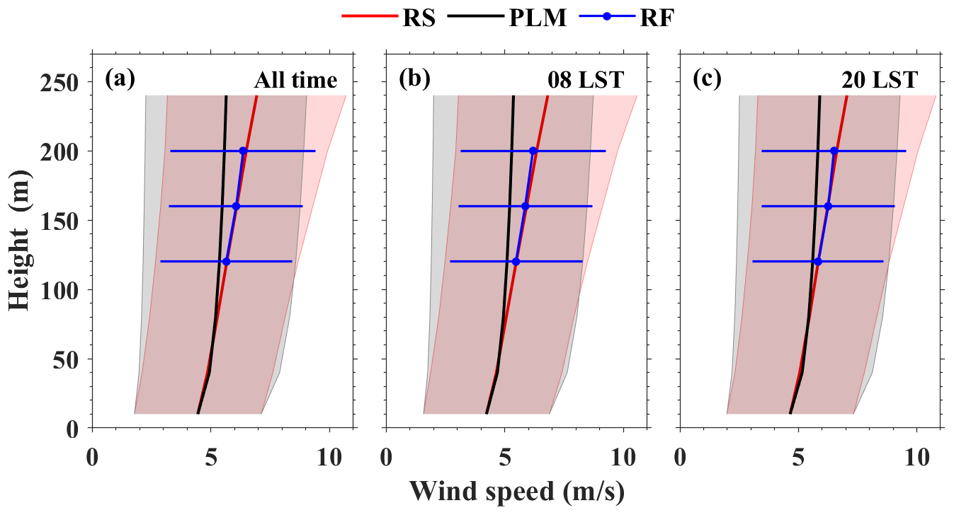
Figure 4 Vertical profiles of the wind speed from different methods at (a) all times, (b) 08:00, and (c) 20:00 LST. Red, black, and blue lines represent mean wind profile from RS, the PLM, and RF, respectively. Corresponding color shading areas represent the standard deviation.

In addition, for both the PLM and RF, the retrieved wind profile at 20:00 LST is closer to the RS observations. The comparisons between the observed wind speed and the estimated wind speed for the PLM and RS at different times are shown in Fig. S7. The fitting results of the PLM and RF at 20:00 LST are slightly higher than those at 08:00 LST. It indicates that the performance of the PLM and RF vary with the hour of the day. This is because the wind profile depends not only on the surface friction but also on the atmospheric stratification (Gryning et al., 2007). The surface layer is in an unstable stratification due to heat transfer caused by solar radiation during daytime, while the surface layer tends to stabilize stratification due to surface radiation cooling during nighttime (Yu et al., 2022; Solanki et al., 2022). WS₁₂₀, WS₁₆₀, and WS₂₀₀ are more vulnerable to the surface turbulence due to the unstable stratification during daytime. Therefore, the performance of the PLM and RF at nighttime is better than that during daytime.

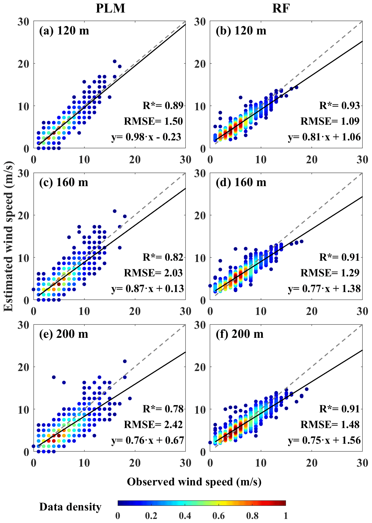
Figure 5 Comparisons between observed wind speed and estimated wind speed for (a, c, e) the PLM and (b, d, f) RF at 120, 160, and 200 m. The gray and black lines are the reference and regression lines, respectively. The color bar represents the data density. The asterisk indicates that the correlation coefficient (R) has passed the t test at a confidence level of 95 %.

Figure 6 shows the comparisons between the observed results and the estimated results for the PLM and RF in different seasons. The red, green, blue, and black represent the spring, summer, autumn, and winter, respectively. At three heights, the performance of the PLM is the best in winter and the worst in summer. It shows that the performance of the PLM is affected by seasonal factors, which is due to the wind shear varying dramatically with the season (Banuelos-Ruedas et al., 2010). Pérez et al. (2005) indicate that the surface-layer wind speed profile is mainly affected by the convection produced by surface heating in summer. WS₁₂₀, WS₁₆₀, and WS₂₀₀ are affected by the surface due to the unstable stratification, which leads to the PLM performing the worst in summer. In contrast, during winter, the surface temperature is generally lower than the air temperature aloft creating a stable inversion (Yu et al., 2022; Liu et al., 2022). WS₁₂₀, WS₁₆₀, and WS₂₀₀ are disconnected from the surface due to stable stratification. It leads to the PLM performing the best in winter. As for RF, although the performance in spring is slightly lower than that in other seasons, the fitting results for the four seasons are significantly improved compared with the PLM. This indicates that RF is the least affected by seasons. The reason is that the RF model is less subjective than the PLM because they are data driven. Overall, in terms of stability and accuracy, RF is more suitable for estimating wind speed at hub height.

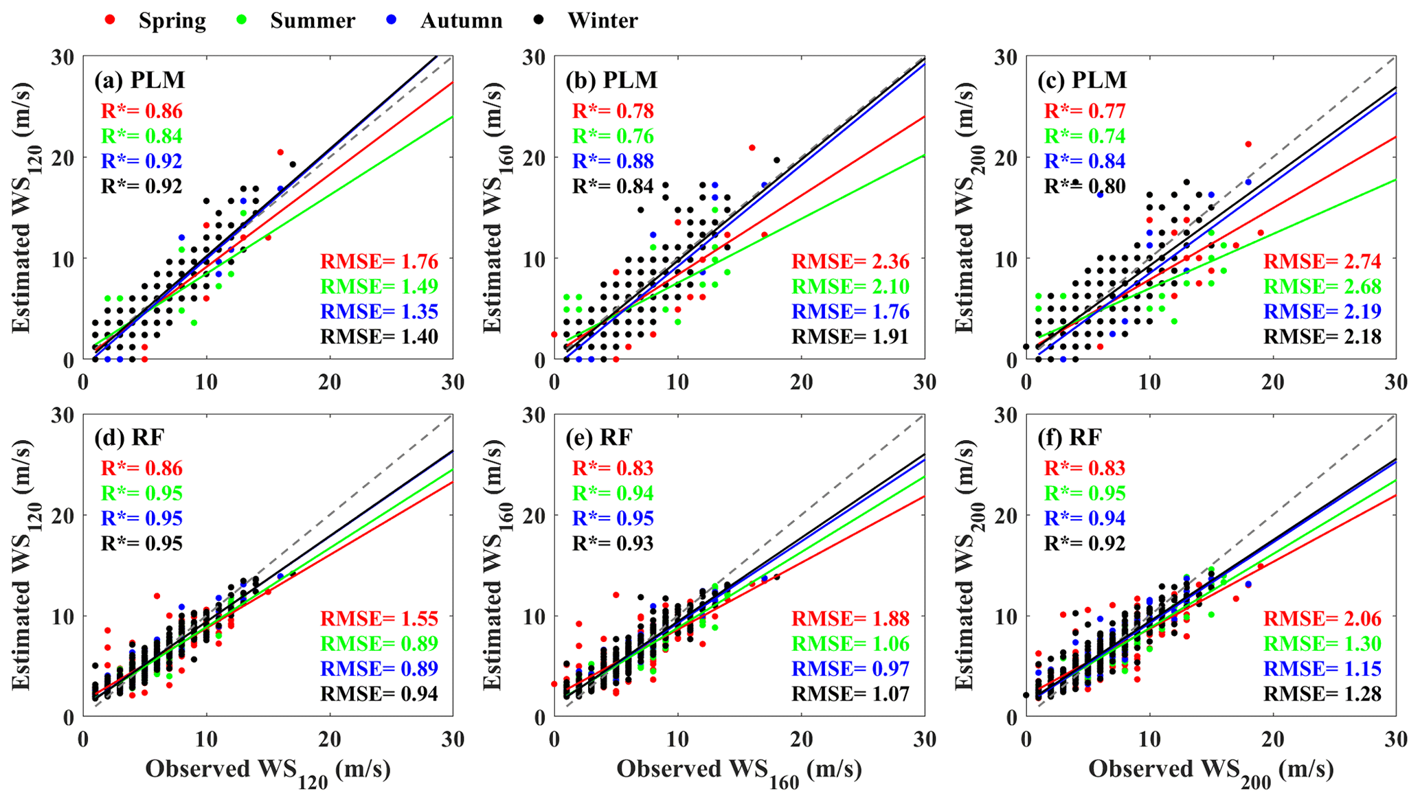
Figure 6 Comparisons between observed wind speed and estimated wind speed for (a, b, c) the PLM and (d, e, f) RF at 120, 160, and 200 m in different seasons. The red, green, blue, and black represent spring, summer, autumn, and winter, respectively. The asterisk indicates that the correlation coefficient (R) has passed the t test at a confidence level of 95 %.

4.2 Vertical profiles of wind speed at surface layer

Figure 7 shows the diurnal and seasonal variations in WS₁₂₀, WS₁₆₀, and WS₂₀₀. The diurnal and seasonal variations in wind speed at three heights are on average similar to each other. From the perspective of daily variation, the wind speed is larger during daytime from 09:00 to 16:00 LST, while it is lower at nighttime from 00:00 to 04:00 LST. This daily cycle is mainly affected by the solar radiation and the sea–land breeze. On the one hand, the surface is heated by solar radiation during daytime, warming the low-level air. The convection formed by the rising warm air mass results in high wind speed during the daytime. After sunset, the surface radiation cools and the air layer tends to stabilize, resulting in a gradual decrease in wind speed (R. Liu et al., 2018). On the other hand, the difference in specific heat capacity between sea and land can form the difference in thermal properties between sea and land. The difference in air pressure is obvious, which is easy to form sea–land breezes (Li et al., 2020). Similar diurnal variations in 10 m wind speed are also observed at three other stations in China (Liu et al., 2013). From the perspective of seasonal variation, the wind speed is large in spring and winter and is low in summer and autumn. This is because the influence of the East Asian Monsoon and Mongolian cyclones (Yu et al., 2016; Zheng et al., 2020). The large-scale synoptic systems in China have a relatively high occurrence frequency during the cold season (spring and winter), which results in the higher wind speed than in the warm season (summer and autumn) (F. Liu et al., 2019).

Figure 7 Monthly and diurnal cycles of (a) WS₁₂₀, (b) WS₁₆₀, and (c) WS₂₀₀ from 1 May 2018 to 31 August 2020. The color bar represents the wind speed from the RF model.

The histograms of WS₁₂₀, WS₁₆₀, and WS₂₀₀ with corresponding Weibull distributions are plotted in Fig. 8. The blue bar and pink lines represent occurrence probability and Weibull distributions, respectively. Moreover, the mean wind speed and Weibull distribution parameters for three heights are listed in Table 1. The occurrence probabilities of WS₁₂₀, WS₁₆₀, and WS₂₀₀ are the unimodal distribution, with a peak probability at medium wind speed (about 5 m s⁻¹) and a low probability at high and low wind speeds. The mean WS₁₂₀, WS₁₆₀, and WS₂₀₀ are 5.84, 6.26, and 6.57 m s⁻¹, which gradually increase with height. The lower wind speed near the ground is caused by the influence of underlying surface roughness and surface friction (Li et al., 2018, 2020). In addition, there is a deviation between the probability density function and the frequency of occurrence at some stations, which is because the Weibull distribution generally has a long tail effect or a right-skewed distribution (Pishgar-Komleh et al., 2015; Ali et al., 2018). Overall, the Weibull distribution matches with the frequency of wind speed at all stations. Therefore, the Weibull distribution parameters can be applied for the wind energy assessment.

Table 1 Statistics for the Weibull distribution of WS₁₂₀, WS₁₆₀, and WS₂₀₀ from 1 May 2018 to 31 August 2020.

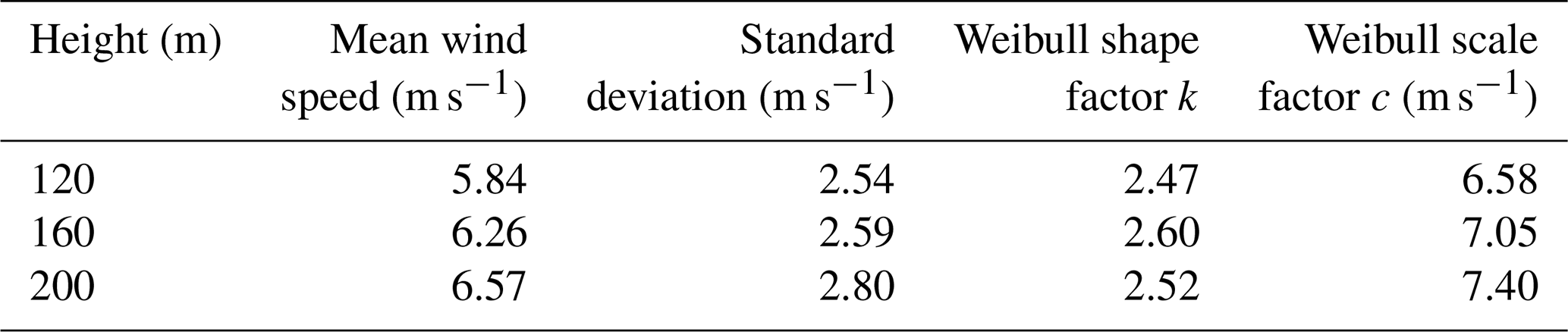
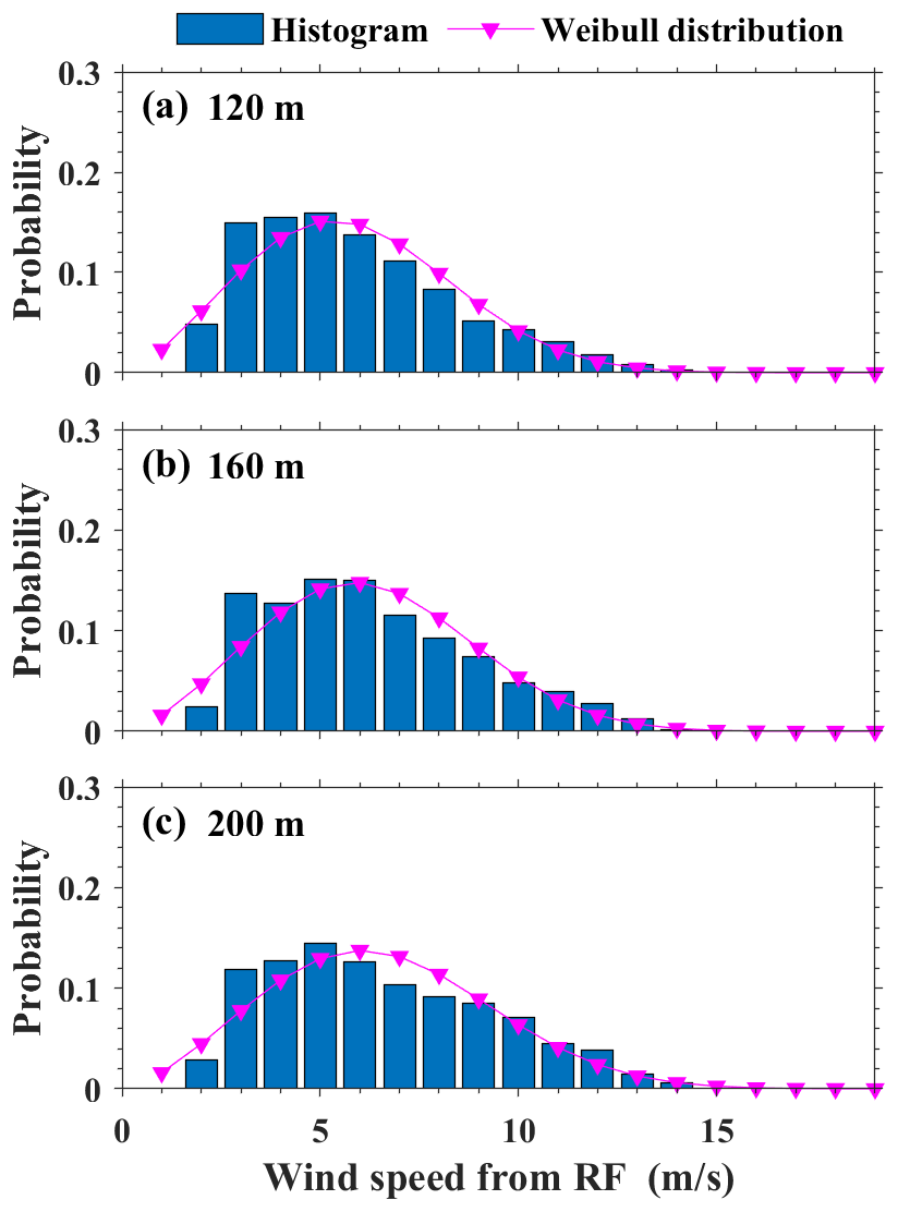
Figure 8 Probability distribution and Weibull distribution of (a) WS₁₂₀, (b) WS₁₆₀, and (c) WS₂₀₀ from 1 May 2018 to 31 August 2020. The blue bar and pink lines represent occurrence probability and Weibull distributions, respectively.

4.3 Influence of wind speed from different methods on WPD

Figure 9 shows the diurnal variations in WPD from the PLM and RF at 120, 160, and 200 m a.g.l. The solid and dotted red lines represent the variation in WPD from RF and the PLM, respectively. The gray bar represents the APE of WPD between RF and the PLM. The diurnal pattern of WPD from RF is like that from the PLM. At three heights, the hourly mean WPD is larger during daytime from 09:00 to 16:00 LST with a peak at 14:00 LST and is lower at nighttime from 00:00 to 04:00 LST. On the contrary, the APE is lower during daytime (08:00 to 18:00 LST) and larger at nighttime (20:00 to 06:00 LST). At 120 m, the mean APEs during daytime and nighttime are 14.09 % and 35.80 %, respectively. Considering that the results from RF are underestimated at high-wind-speed conditions, the APE of WPD between the PLM and actual observations during daytime should be slightly greater than 14.09 %. Moreover, the diurnal variations in APE at 160 and 200 m a.g.l. generally resemble the features obtained at 120 m a.g.l. But the APE of WPD between RF and the PLM increases with the height. These results indicate that the PLM is more suitable for wind energy assessment in the daytime, and the error in wind energy assessment based on the PLM is gradually increased as the height increases.

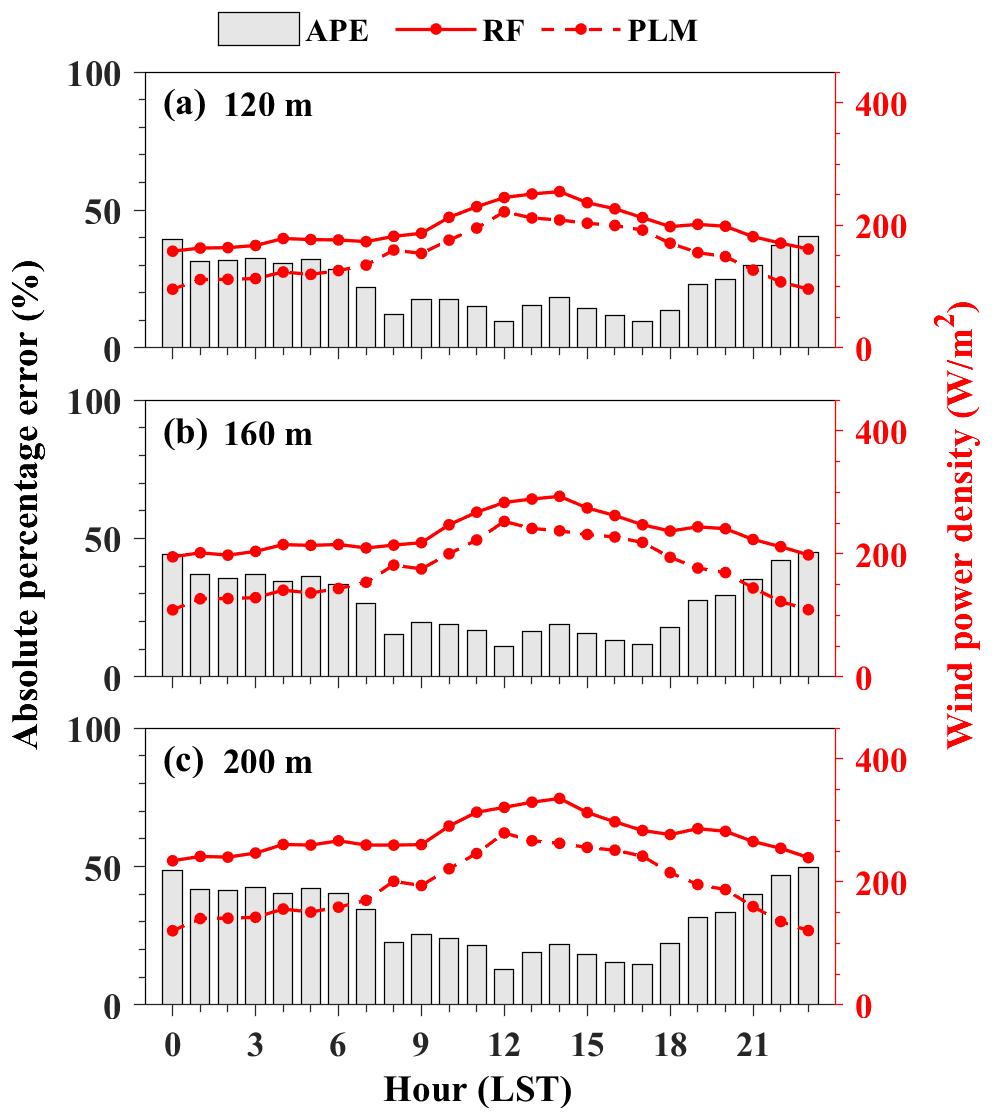
Figure 9 Diurnal variation in the wind power density (WPD) at (a) 120 m, (b) 160 m, and (c) 200 m. The solid and dotted red lines represent WPD from RF and the PLM, respectively. The gray bar represents the absolute percentage error (APE) of WPD between RF and the PLM.

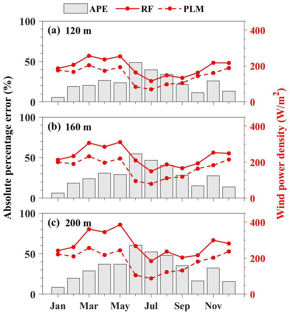
Figure 10 shows the monthly variations in WPD from the PLM and RF at 120, 160, and 200 m a.g.l. The monthly variation in WPD from RF is also similar to that from the PLM. The monthly WPD is relatively high for the period from March to May, as compared to the lower values from June to October. At 120 m, the APE is largest in summer and is lowest in winter. The seasonal APEs during spring, summer, autumn, and winter are 23.65 %, 40.83 %, 19.67 %, and 12.62 %, respectively. The monthly variations in APE at 160 and 200 m are consistent with that at 120 m. It indicates that the PLM is more suitable for wind energy assessment in autumn and winter. In addition, the APEs during spring at 120, 160, and 200 m are 23.65 %, 28.12 %, and 34.22 %, respectively. Due to the performance of the RF model being the worst in spring, the APE of WPD between the PLM and the real value during spring may increase. Jung et al. (2021) also find that the global median absolute percentage error in the wind energy estimations is 36.9 % assuming the power law exponent is 0.14. Overall, the PLM has some limitations in wind energy assessment above 100 m. When using the PLM to evaluate wind energy at a greater height, it is necessary to pay attention to its errors. Moreover, the use of an RF model that takes the factors such as surface friction, heat transfer, and upper-height wind speed constraints into account is suggested to evaluate wind energy.

Figure 10 Similar to Fig. 9 but for the monthly variation.

5 Summary and conclusions

The traditional methods such as the PLM used to estimate wind speed at hub height generally assume a constant exponent α in establishing the power law relationship between wind speeds at surface and hub height, which inevitably leads to large uncertainties. To confront this challenge, this study uses the RF algorithm to retrieve the wind profile based on the RWP and surface meteorological data from May 2018 to August 2020.

The comparison against observations indicates that WS₁₂₀ values estimated from RF are better than those from the PLM given the relatively higher R (0.93 versus 0.89) and smaller RMSE (1.09 m s⁻¹ versus 1.50 m s⁻¹). Particularly, the performance of the PLM declines with height. Especially at 200 m, the R and RMSE from the PLM change to 0.78 and 2.42 m s⁻¹, respectively. In contrast, the RF model maintains good accuracy at different heights. The R (RMSE) values for the RF model at 160 and 200 m are 0.91 (1.29 m s⁻¹) and 0.91 (1.48 m s⁻¹), respectively. These results show that above the surface layer, the wind speeds from the PLM deviate from the observed value. The RF model is more suitable for retrieving the hub-height wind speed when the hub height is extended above the surface layer. Overall, the RF model shows advantages over the traditional PLM. This is because the RF model considers well the influence of near-surface environmental parameters, such as friction velocity and Charnock coefficient. Moreover, the heat transfer and upper-height wind speed constraints are also considered in the construction of the RF model. Based on the wind speed from RF, the diurnal and seasonal variations in wind energy are then analyzed. The hourly mean WPD is larger from 09:00 to 16:00 LST with a peak at 14:00 LST. WPD is relatively high in spring and winter, as compared to the lower values in summer and autumn. Finally, the differences in WPD between RF and the PLM at different heights are investigated. At 120 m, the mean APEs of WPD between RF and the PLM during daytime and nighttime are 14.09 % and 35.80 %, respectively. Moreover, the seasonal APE at 120 m is largest in summer (40.83 %) and is lowest in winter (12.62 %). In addition, the mean APEs at 120, 160, and 200 m are 24.19 %, 27.99 %, and 32.57 %, respectively. These results indicate that there are some errors in the wind energy evaluation based on wind speed from the PLM. Therefore, when retrieving upper-height wind speed, it is suggested to combine more observation or auxiliary data to build a more accurate model, such as an RF model. In the absence of other observation data, it is necessary to pay attention to the errors when using the PLM to evaluate wind energy at greater heights.

Our work provides a new pathway to fill the data gap of wind speed at the hub height for the high capability of the state-of-the-art ML algorithm, which lays a solid foundation for more robust wind energy assessments. However, the high-precision wind profile estimate is only one part of the efficient utilization of wind energy resources. The cost of wind turbines, topography conditions, and other factors also need more attention, which deserves further investigation in the future.