the Creative Commons Attribution 4.0 License.
the Creative Commons Attribution 4.0 License.
 | 09 Mar 2023
Indicators of the ozone recovery for selected sites in the Northern Hemisphere mid-latitudes derived from various total column ozone datasets (1980–2020)
Janusz Krzyścin
We propose a method to examine the current status of the ozone recovery attributed to changes of ozone-depleting substances (ODS) in the stratosphere. The total column ozone (TCO3) datasets used are based on the ground-based (by the Dobson and/or Brewer spectrophotometer) measurements, satellite observations (from the Solar Backscatter Ultraviolet (SBUV) and Ozone Mapping and Profiler Suite (OMPS) instruments), and output of reanalyses (Multi-Sensor Reanalysis version 2 (MSR2) and Modern-Era Retrospective Analysis for Research and Applications, version 2 (MERRA2)). The TCO3 time series are calculated for selected sites in the mid-latitudes of the Northern Hemisphere (NH, 35–60∘ N), which are station locations with long-term TCO3 observations archived at the World Ozone and Ultraviolet Radiation Data Centre (WOUDC). The TCO3 monthly means (1980–2020) are averaged over the April–September period to obtain TCO3 time series for the warm sub-period of the year. Two types of the averaged TCO3 time series are considered: the original one and non-proxy time series with removed natural variability by a standard multiple regression model. The TCO3 time series were smoothed by the locally weighted scatterplot smoother (LOWESS) and the super smoother (SS). The smoothed TCO3 values in 1980, 1988, 1997, and 2020 were used to build ozone recovery indices (ORIs) in 2020. These are key years in the equivalent effective stratospheric chlorine (EESC) time series for the period 1980–2020, i.e., the stratosphere was only slightly contaminated by ODS in 1980, 1988 is the year in which the EESC value is equal to its value at the end (2020), and in 1997, the EESC maximum was in mid-latitude stratosphere. The first proposed ORI, ORI1, is the normalized difference between the TCO3 values in 2020 and 1988. The second one, ORI2, is the percentage of the recovered TCO3 in 2020 since the ODS maximum. Following these definitions, the corresponding reference ranges (from −0.5 % to 1 % for ORI1 and from 40 % to 60 % for ORI2) are obtained by analyzing a set of possible EESC time series simulated via the Goddard automailer. The ozone recovery phases are classified comparing the current ORI values and their uncertainty ranges (by the bootstrapping) with these reference ranges. In the analyzed TCO3 time series, for specific combinations of datasets, data types, and the smoother used, we find faster (for ORI1 or ORI2 above the reference range) and slower (for ORI1 or ORI2 below the reference range) recovery in 2020 than that inferred from the EESC change, and a continuation of the TCO3 decline after the EESC peak (ORI2<0 %). Strong signal of the slower TCO3 recovery is found in Toronto, Hohenpeissenberg, Hradec Kralove, and Belsk. A continuation of ozone decline after the turnaround in ODS concentration is found in both the original and non-proxy time series from WOUDC (Toronto), SBUV and OMPS (Toronto, Arosa, Hohenpeissenberg, Uccle, Hradec Kralove, and Belsk), and MERRA2 data (Arosa, Hohenpeissenberg, Hradec Kralove, and Belsk).
- Article
(4850 KB) - Full-text XML
- BibTeX
- EndNote


Unexpected low total column ozone (TCO3) values observed in the early 1980s over Antarctica alarmed both scientists and public because of anticipated increase of ultraviolet radiation (UVR) reaching the Earth's surface (Chubachi, 1984; Farman et al., 1985; Solomon et al., 1986). Widespread threats of thinning of the stratospheric ozone layer and corresponding danger for the Earth's environment led to signing the Montreal Protocol (MP) in 1987 to phase out the man-made ozone-depleting substances (ODS). Overturning of the ODS concentration in the stratosphere (from large increase since the early 1980s to slight decrease beginning in the mid-1990s) was an evident sign of the success of MP and its subsequent amendments. The ODS turnaround in the stratosphere was observed around the middle 1990s in the mid-latitudes and at the beginning of the 2000s in Antarctica. This also triggered numerous studies to reveal the corresponding change point in TCO3 trends to support the impact of the MP and its later amendments on the ozone layer (e.g., Reinsel et al., 2005; Mäder et al., 2007; Harris et al., 2008; Weber et al., 2018).
Trends in ozone were usually calculated using multiple linear regression (MLR) with a number of proxies to eliminate TCO3 variations related to dynamical oscillations in the atmosphere, the 11-year solar activity, and volcanic eruptions. The anthropogenic component of the trend term was usually modeled as independent (disjoint) or dependent (joint) two lines drawn for the periods of increasing and decreasing ODS concentration in the stratosphere (e.g., Weber et al., 2018). There were only a few papers using a non-linear smoothed trend pattern based on the dynamical linear model (Laine et al., 2014; Maillard Barras et al., 2022), Fourier series (Bozhkova et al., 2019), and other smoothers, e.g., locally weighted scatterplot smoothing (LOWESS) by Krzyścin and Rajewska-Więch (2016) and wavelets by Delage et al. (2022).
Coldewey-Egbers et al. (2022) calculated latitude–longitude linear TCO3 trends since 1995 over the entire globe based on the satellite data record. The trends in the mid-latitudes of the Northern Hemisphere (NH) were mostly insignificant. In some isolated regions, they found statistically significant trends, e.g., negative in East Europe and positive in the northern part of the North Atlantic. This pattern was linked with the opposite trends in the tropopause height. A continuation of the TCO3 declining tendency since the ODS turnaround was surprisingly revealed in the lower stratosphere of the NH (Ball et al., 2018). A rather positive trend was expected due to a strengthening of the Brewer–Dobson circulation that was suggested by chemistry–climate models (e.g., Dietmüller et al., 2021). The negative trends in the NH lower stratosphere might be attributed to enhanced horizontal air mass exchange with the tropical region less abundant with ozone in the lower stratosphere (Thompson et al., 2021). However, other studies using observational data did not reveal such decline in the NH lower stratospheric ozone, mostly due to large uncertainty in the satellite observations (e.g., Arosio et al., 2019).
The NOAA proposed the ozone-depleting gas index (ODGI) to keep track of changes in ODS concentration in the mid-latitudes and Antarctica (Montzka et al., 2022). Equivalent effective stratospheric chlorine (EESC) was used as a measure of the stratospheric halogen loading, which is weighted by the ozone destruction potential of each gas-depleting stratospheric ozone. The ODGI was defined as an indicator of the EESC current decline since its peak, which is expressed in percentage of the corresponding decline, needed to reach the EESC level in 1980, when ODS concentration in the stratosphere was only slightly affected by man-made substances. The EESC peak year in the mid-latitude stratosphere was found in 1997, being 3 years later than the ODS peak in the troposphere (Montzka et al., 2022). The corresponding ODGI value in 2020 was 51.7 %, providing almost half of the reduction of EESC necessary to reach its undisturbed level existing in 1980. This also provided an estimate of the recovery time around 2045 in the mid-latitudes if factors affecting ODS changes were the same as those in the period 1997–2020. In addition, the EESC level in 2020 corresponds to the 1988 level (Fig. 1).
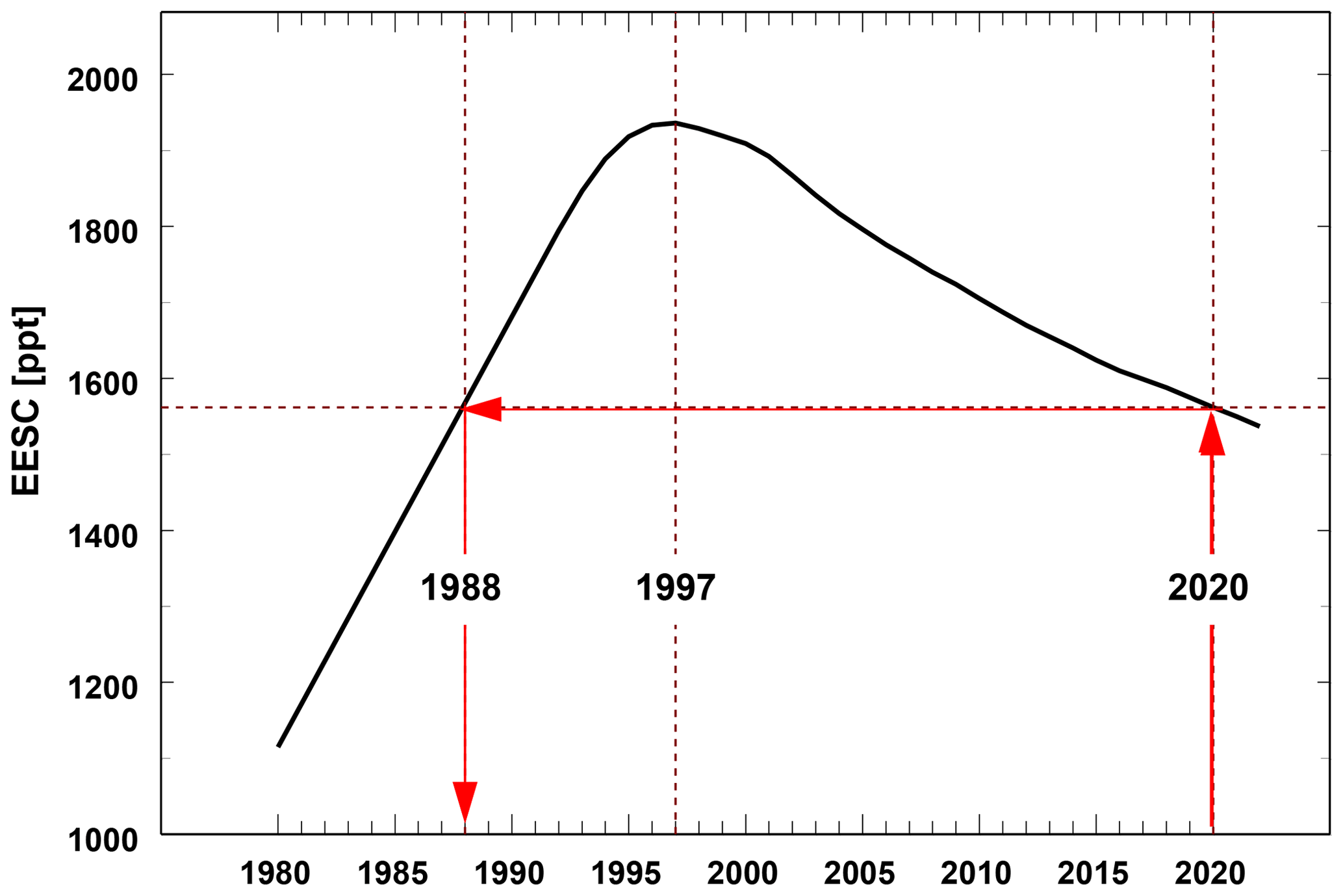
Figure 1The EESC time series with marked key years: the EESC maximum in 1997 and 1988 when the EESC value was the same as in 2020 (the end of total column ozone data used in the paper) based on the EESC pattern proposed by Montzka et al. (2022).
Following the ODGI concept, we propose indices to monitor ozone recovery attributed to the EESC changes using various TCO3 datasets from ground-based and satellite observations and two reanalyses. These indices will be calculated for selected NH mid-latitudinal sites corresponding to locations of the ground-based stations with long-term time series archived in the World Ozone and Ultraviolet Radiation Data Centre (WOUDC). From the smoothed pattern of long-term TCO3 changes, we will extract TCO3 values in key years: 1980, 1988, 1997, and 2020 (Fig. 1). These four values will be used to calculate the proposed ozone recovery indices (ORIs) showing the current stage of the stratospheric ozone recovery. The Goddard automailer (http://acdb-ext.gsfc.nasa.gov/Data_services/automailer/index.html, last access: 27 February 2023) will be implemented to simulate various possible EESC patterns to estimate variability of the EESC peak year and the year when the EESC value is equal to its value in 2020.
In Sect. 2, the TCO3 datasets are presented. In Sect. 3, the data preparation, ORI definition, and a method to obtain the uncertainty range of the ORI estimate are described. Section 4 presents ORI values for selected mid-latitudinal sites for various datasets using combinations of the data smoother and data category. In Sect. 5, the discussion and conclusions are presented.
Table 1Selected ground-based total column ozone observing stations in the NH mid-latitudes with the data record archived in WOUDC.
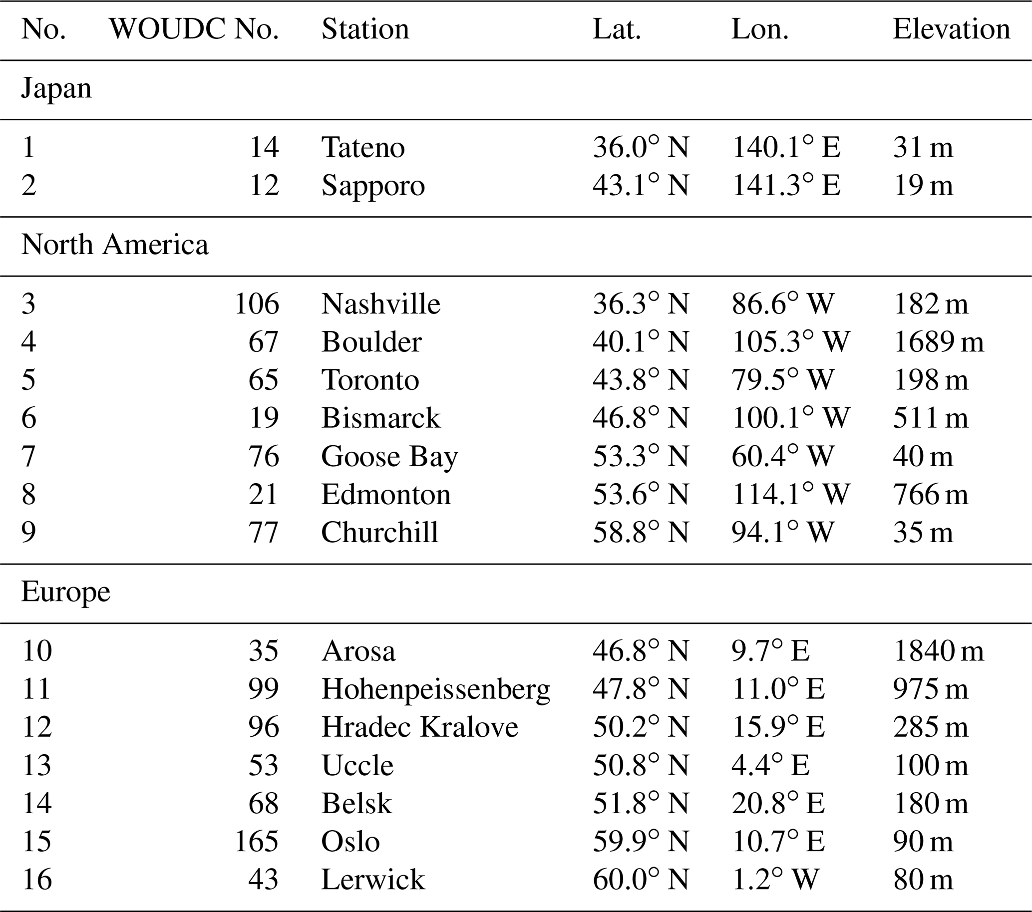
Four TCO3 datasets are used in the study from ground-based and satellite observations as well as from two reanalyses. The TCO3 time series are calculated for selected sites in the NH mid-latitudes (35–60∘ N) corresponding to locations of stations that archived results of the ground-based observations by the Dobson and/or Brewer spectrophotometer at WOUDC. Arosa and Davos datasets were combined since the ozone monitoring at Arosa was moved to the nearby station Davos in 2014. Sixteen stations with long-term and continuous observations (starting at least before 1980 and ending after 2020) are selected (Table 1). The monthly mean TCO3 values for these stations are taken from the WOUDC website.
The NASA Merged Ozone Data (MOD) version 8.7 is used for a comparison with the WOUDC data. An overpass subset of MOD provides daily means of ozone content in various stratospheric layers and column ozone over the WOUDC sites including also those listed in Table 1. The MOD time series are built using the homogenized spectral measurements of the solar backscattered UV on various satellite platforms: Nimbus 4, Nimbus 7, NOAA 9, 11, 14, 16, and 17–19, and Suomi National Polar-orbiting Partnership (NPP) (Frith et al., 2014; Weber et al., 2022).
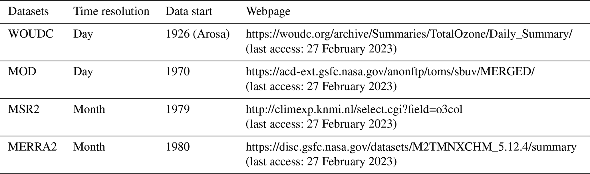
Two other datasets represent the category of reanalyzed data, i.e., the global TCO3 field taken from output of 3-D chemistry and transport models. Here, we examine time series for the selected sites interpolated from the Multi-Sensor Reanalysis, version 2 (MSR2) global data with the resolution (van der A et al., 2015) and Modern-Era Retrospective analysis for Research and Applications, version 2 (MERRA2) with the 0.5∘ (latitude) × 0.625∘ (longitude) resolution (Wargan et al., 2017). Table 2 presents the sources of all datasets used in the study.
The TCO3 monthly means from all datasets described in Sect. 2 are averaged over the warm sub-period of the year (April–September) to build seasonal TCO3 time series (1980–2020) for all NH mid-latitudinal selected sites listed in Table 1. The dynamic variability of ozone in these months is much smaller than in the cold sub-period of the year, so the variability of TCO3 is lower and chemical changes are potentially more pronounced. Moreover, ground-based TCO3 observations are the most accurate during this part of the year due to the Sun's high elevations and better weather conditions, allowing the most reliable ozone observations with spectrophotometers (Komhyr, 1980).
During the warm sub-period of the year, UVR is much higher compared to the cold sub-period. Having a detrimental effect on the Earth's ecosystems, UV overexposure is most frequent in the warm sub-period of the year. Therefore, analysis of the long-term TCO3 changes during this period of the year is of special importance to discuss detrimental biological effects of the ozone changes. In the mid-1980s, the anticipated risks of UV overexposure led to international initiatives to protect the ozone layer. In addition, the results based on the entire year (January–December) and the cold sub-period (October–next year March) data are presented in Appendix A.
3.1 Data smoother
Two data smoother types are examined in the study: LOWESS by Cleveland (1979) and super smoother (SS) by Friedman (1984). Here, for the LOWESS application, the smoothness level is pre-defined to have up to two turning points in the smoothed time series, i.e., the smoothing parameter f is set equal to 0.5. The first turning point corresponds to the ODS turning point in 1997 and the next point is set to reveal a change of the recovery rate after 1997 (if it exists). For SS, we use an option with no pre-defined smoothness level. The smoothed curve is obtained by means of a bivariate regression smoother based on local linear regression with adaptive bandwidths. Figure 2 illustrates the performance of both smoothers applied to the time series of seasonal (April–September) TCO3 means for Tateno and Toronto from the ground-based observations.
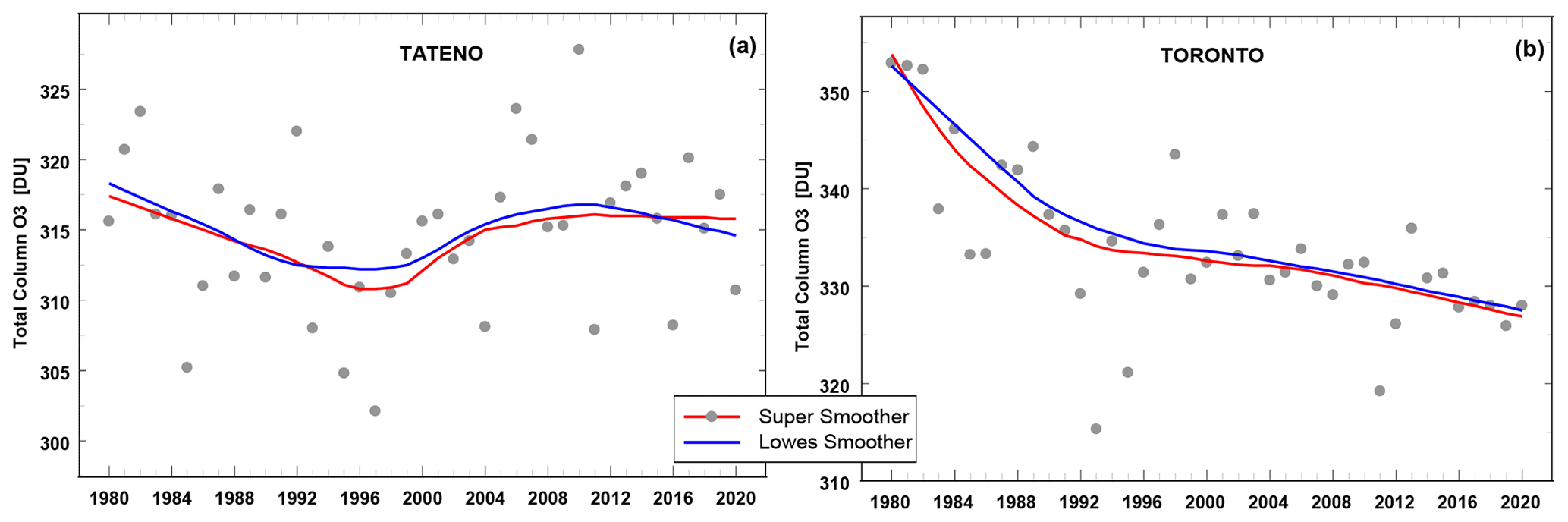
Figure 2Examples of the long-term time series of total column ozone from ground-based observations in the warm sub-period (April–September) by locally weighted scatterplot smoother (blue curve) and super smoother (red curve): Tateno (a), Toronto (b).
3.2 Removal of the ozone natural variability
The smoothed pattern of TCO3 time series is used to discuss long-term variability in the series comprising 41 yearly values. The smoothers described in Sect. 3.1 are applied to both original time series and the series with removed variability due to various dynamical–chemical processes not directly involved with the anthropogenic emission of chemicals affecting the stratospheric ozone. Various proxies (explanatory variables in MLR) for these “natural” processes have been proposed by parameterizing dynamical–chemical forcing on the ozone layer. Frequently in MLR, the solar activity cycle (e.g., 10.7 cm solar radio flux), indices of internal atmospheric fluctuations (quasi-biennial oscillations, El-Niño Southern oscillations, and Arctic oscillations), optical depth of the stratospheric aerosols, and the eddy heat flux in the stratosphere (to parameterize the intensity in the Brewer–Dobson circulation) were used. The proxy set proposed by Weber et al. (2022) is used here with the sources listed in their Table 2. The only differences between our proxy set and that of Weber et al. (2022) are using the eddy heat flux at 100 hPa from the NASA Atmospheric Chemistry and Dynamics Laboratory database (https://acd-ext.gsfc.nasa.gov/Data_services/met/ann_data.html, last access: 27 February 2023) and the stratospheric aerosol optical depth updated from Sato et al. (1993) for the entire time data (i.e., no different aerosol data sources after 1990).
The standard MLR with two independent linear trend terms (before and after the year of ODS turnaround) is used to extract the trend pattern and the combined signal due to all proxies. The MLR used here is identical to the one labeled as full MLR in Weber et al. (2022). Finally, the TCO3 time series combining proxy signals is subtracted from the original time series to obtain the TCO3 series containing only the anthropogenic long-term component and noise. Further in the text, this time series is called non-proxy times series.
3.3 Ozone recovery index
The proposed ozone recovery indices (ORIs) follow the ODGI concept (Montzka et al., 2022) of using selected values from the EESC series to define the recovery status. Key TCO3 values are taken at the beginning (1980), at the end of the data (2020), in the year of TCO3 trend overturning (1997), and in the year (1988) when the EESC value in the NH mid-latitudes was the same as in 2020. Last two years are taken according to the EESC pattern shown in Fig. 1. Smoothed TCO3 values in the selected key EESC years T, in the EESC pattern, which are denoted as , , are used for calculation of the following dimensionless ORIs in 2020:
If the ozone recovery follows ODS changes, ORI1(1988,2020) will be equal to 0 % but negative (positive) for slower (faster) TCO3 recovery than that found in the EESC pattern. Correspondingly, the ORI2(1997,2020) value in the Northern Hemisphere will be equal to 48.3 % (i.e., 100 % – ODGI(2020), see ODGI(2020) = 51.7 % in Montzka et al., 2022) if the ozone recovery in the period 1980–2020 follows EESC changes and lower (higher) than this reference value if the ozone recovery is slower (faster) compared to that existing in the EESC.
If ORI2(1997,2020) is less than 0 % and the ozone is declining before the ODS overturning year (usual case for the NH mid-latitudinal TCO3), the ozone depletion will also continue after the EESC overturning. It is worth mentioning that for a searching of the TCO3 recovery over Antarctica in 2020, the smoothed TCO3 values in 1980, 1993, 2001, and 2020 need to be selected as these years correspond with key years in the EESC pattern for this region (Montzka et al., 2022).
3.4 ORI reference range
The specific EESC pattern, which is shown in Fig. 1, was used in the calculation of ODGI and the year when EESC was equal to its value in 2020. Various shapes of the EESC pattern can be provided via the Goddard automailer depending on parameters characterizing ODS in the stratosphere: mean age of air, age of air spectrum width, Bromine scaling factor, and the fractional release type. For mid-latitudes, the default values in the automailer are 3 years and 60 for the mean age of the air and the Bromine scaling factor, respectively. We examine two additional options, i.e., 3.3 years and 2.7 years and 45 and 75, based on the uncertainties (1σ) of these parameters discussed by Velders and Daniel (2014) for mid-latitudes (see their Table 2). Moreover, two options are assumed for age of air spectrum width, i.e., 1.5 years (default in the automailer) and 3 years (arbitrarily selected). Moreover, three types of the fractional release type are implemented: Newman et al. (2006), Laube et al. (2010), and default type denoted as WMO_2010. In total, 54 EESC patterns have been obtained. Figure 3a shows the EESC's peak values and the corresponding years at the EESC maxima derived from the automailer together with the pair (1936 ppt and 1997) used in ODGI calculations by Montzka et al. (2022). The range of 100 %–ODGI(2020) values (equivalent to ORI2(1997,2020) obtained with the corresponding EESC values instead of TCO3 in Eq. 2) is from 40 % to 60 % using all simulated EESC curves (Fig. 3b). This gives the reference range for ORI2(1997,2020) when the ozone recovery is similar to that of the EESC.

Figure 3The EESC characteristics derived via the Goddard automailer (open circles) and those (full circles) taken from Montzka et al. (2022): EESC maximum value versus the year at the peak (a), ORI2(1997,2020) value calculated on the basis of the EESC values in Eq. (2) (equivalent to 100 %–ODGI(2020)) versus the year when the EESC value is equal to that in 2020 (b).
The year (before the EESC peak) T when EESC was equal to its value in 2020 changes from 1986 to 1989 (Fig. 3b). The mean total ozone value, , for this year can be calculated by assuming that the ozone linear trend with rate A (in Dobson unit per year) as almost linear depletion of TCO3 existed in mid-latitudes in the 1980s (e.g., Hudson et al., 2006):
For the earliest (1986) and latest year (1989) shown in Fig. 3b using the definition of T, , we conclude after simple mathematical manipulations with Eqs. (1) and (3) that ORI1(1988,2020) equals −2 yr A′ and 1 yr A′, respectively, when % is the ozone trend (in percentage) in the 1980s. Earlier studies estimated A′ of a few percent per decade in the NH mid-latitudes (e.g., WMO, 1999; Hudson et al., 2006). Finally, taking A′ of −0.5 % per decade, the reference range for ORI1(1988,2020) can be estimated from −0.5 % up to 1 %.
3.5 Uncertainty of ORI estimates
The original TCO3 time series, TCO3(t) is divided into two parts to account for the long-term variability, , which is extracted by the smoother and the residual parts, Resid_TCO3(t):
For each selected WOUDC station and data type (original or without proxy effects), two smoothers (LOWESS and SS) are applied to extract the long-term variability and the residual part of TCO3 variability comprising the dynamical–chemical part of variations and noise. The uncertainty range (between the 5th and the 95th percentile) of each ORI estimate is calculated from the set of ordered (lowest to highest) synthetic ORI values derived by bootstrapping. This method of calculating uncertainties of the trend estimates has been applied in our previous studies (e.g., Krzyścin et al., 2015).
The first step of bootstrapping is building synthetic nth time series, Resid_, to mimic the residual term in Eq. (4):
The random year tx is obtained by drawing with replacement any year between 1980 and 2020. The total number of the bootstrapped time series used, N=10 000, is derived experimentally to have stable estimates of ORIs. The use of drawing with replacement in the construction of synthetic residuals was allowed because the original residuals were random, which was confirmed by the one-sample Wald–Wolfowitz run test (Wald and Wolfowitz, 1940).
The original and synthetic residuals should be identical in nature, i.e., have almost similar cumulative distribution. The two-sample Wald–Wolfowitz run test is applied to check the difference between the original and synthetic residuals. If the time series of residuals derived by the drawing with replacement was found to be significantly different (with the 95 % confidence) from the original ones, such residuals were not used in the bootstrapping. This means that the number of draws was greater than the total number of the series (N) used in the bootstrap sample.
The next step of the bootstrapping is adding the Resid_ term to the smoothed part of the original TCO3 series to build nth synthetic TCO3(t) time series:
The smoothed nth time series, is obtained by applying LOWESS (or SS) to the synthetic time series. By repeating this procedure, a set of synthetic series, , is constructed.
Finally, for each series, and are calculated using Eqs. (1) and (2), respectively. From the ordered set of and values, the uncertainty range (5th percentile–95th percentile) is obtained. This allows us to discuss if ORIs values are significantly different from the reference ORI ranges (Sect. 3.4) that define the recovery stage, i.e., −0.5 % to 1.0 % and 40 % to 60 % for ORI1(1988,2020) and ORI2(1997,2020), respectively.
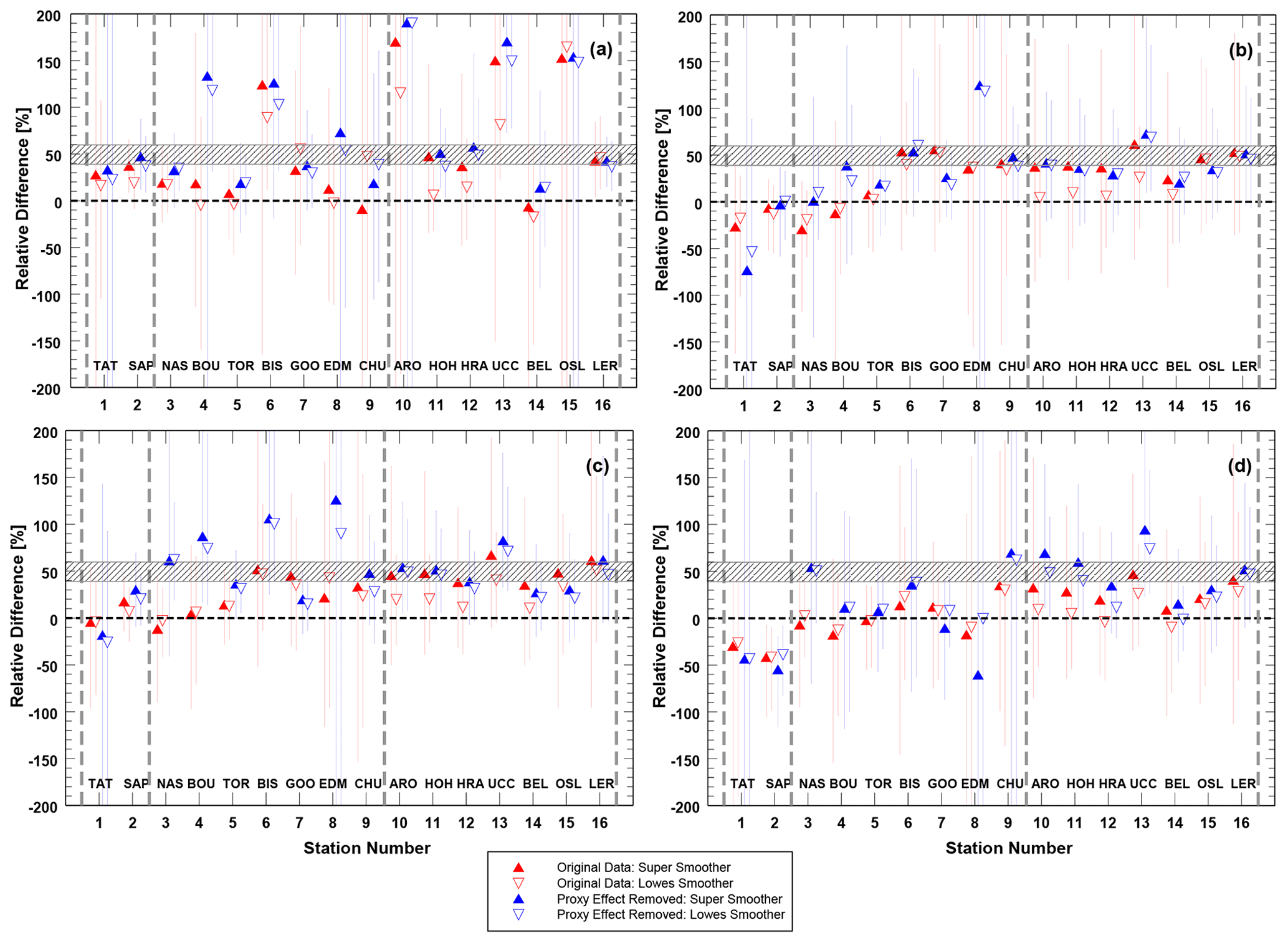
Figures 4–5 illustrate the median and uncertainty range of ORI1(1988,2020) and ORI2(1997,2020), respectively, for all WOUDC stations listed in Table 1. These values are calculated using TCO3 monthly mean values averaged over the warm sub-period of the year. Results are shown in Figs. 4–5 (in panels (a)–(d)) for WOUDC, MOD, MSR2, and MERRA2 data, respectively. The order of the stations on the x axis in these figures is the same as in Table 1, i.e., first, there are two Japanese stations, then, seven North American, and finally, seven European stations. For each region (between the vertical dashed lines), the results are arranged from the southernmost to the northernmost station.
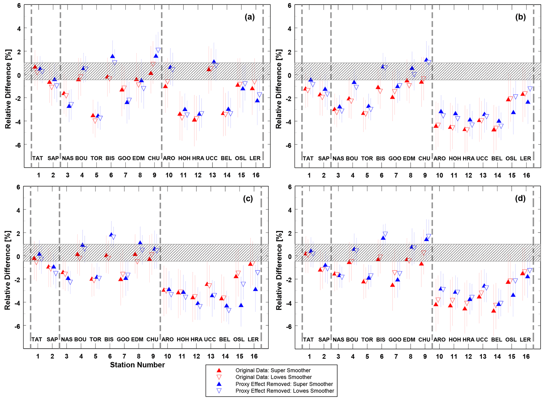
Figure 4Median of the ozone recovery index, ORI1(1988, 2020) estimate (triangle) based on Eq. (1) and its uncertainty range (line) for 16 NH mid-latitudinal stations (Table 1) and various combinations of data smoothers and datasets: WOUDC data (a), MOD data (b), MSR2 (c), and MERRA2 (d). Results in red are for the original data and in blue for the data with removed natural variability. The hatched area marks the reference range, −0.5 % to 1.0 %, calculated in Sect. 3.4.
The location of the uncertainty range of ORIs in Figs. 4–5 relative to its reference range defined in Sect. 3.4 provides the stage of the ozone recovery at each selected station. Namely, if the uncertainty range of ORI is entirely above (below) the reference range, the ozone recovery is faster (slower) than that existing in the EESC for the period 1980–2020. This means that the TCO3 recovery rate is significantly different (at least at the 95 % confidence level) when compared with corresponding EESC values. If the uncertainty range crosses the reference range, the hypothesis of the TCO3 recovery rate following the EESC changes cannot be rejected. The depletion of TCO3 will continue even after the EESC maximum if the uncertainty range for ORI2(1997,2020) is below 0 %. In this case, there is no TCO3 recovery for the entire period (1980–2020).
The ozone recovery is discussed for both the original data and non-proxy time series (with removed combined proxy signal from the original data). A strong signal is when the TCO3 recovery at a selected station is slower (faster) than that found in the EESC if the uncertainty ranges of both ORIs are below (above) the reference ranges for all data types (WOUDC, MOD, MSR2, and MERRA2) and the smoother type used.
Strong support for the slower TCO3 recovery can be found for three European stations: Hohenpeissenberg, Hradec Kralove, and Belsk. For Arosa and Uccle, using ORI2(1997,2020), the slower ozone recovery is found in all datasets except WOUDC. This may suggest a problem with the homogeneity of WOUDC data, at least for Arosa, as the results are different than those obtained at the nearby Hohenpeissenberg station. For Toronto and Nashville, using ORI2(1997,2020) derived from the non-proxy time series, the slower ozone recovery can be suggested.
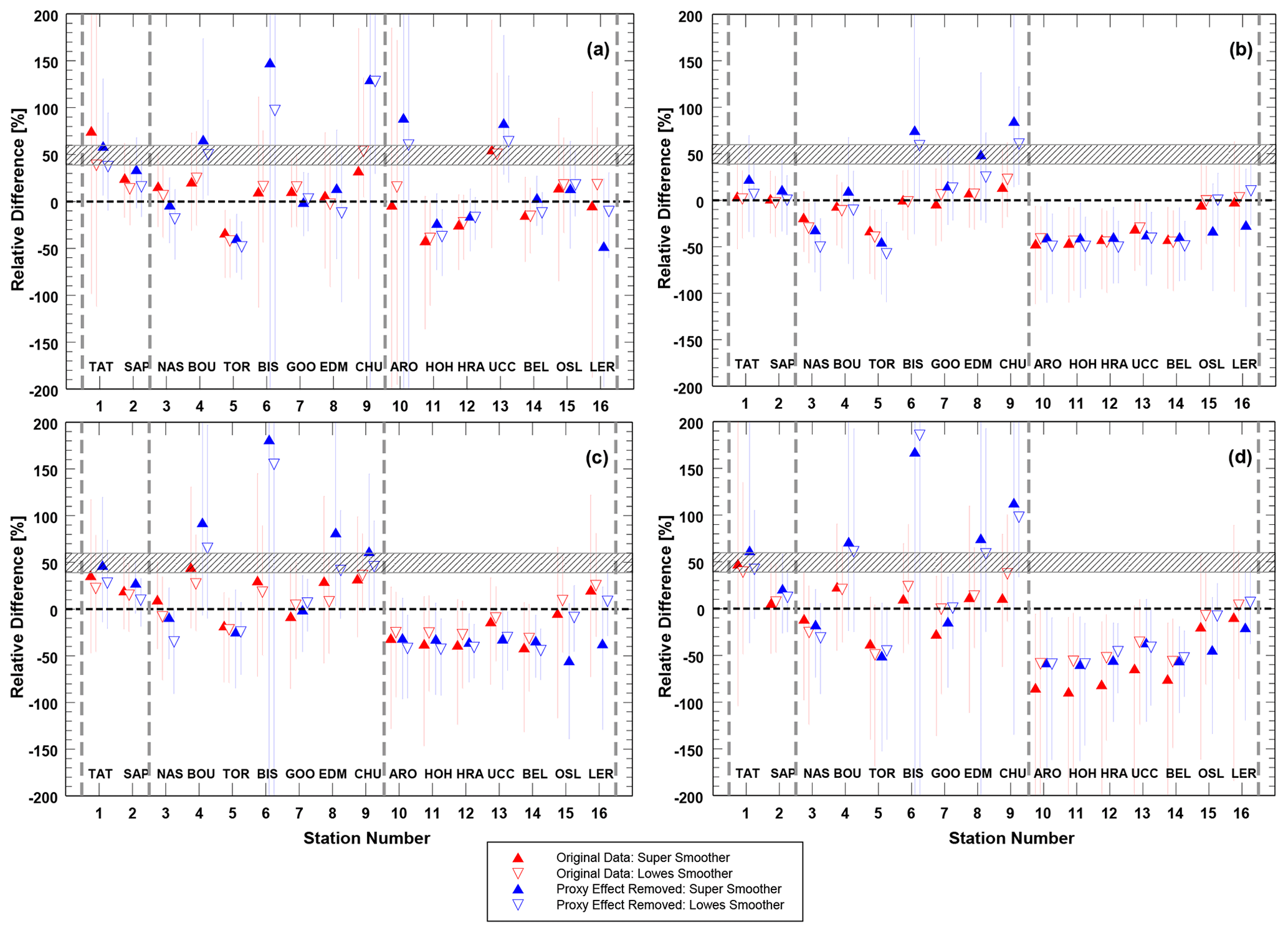
Figure 5The same as Fig. 4 but for the ozone recovery index, ORI2(1997,2020) based on Eq. (2). The reference range (hatched area) is between 40 % and 60 % according estimates in Sect. 3.4.
There are many individual cases where the localization of the uncertainty range of the ORI estimate suggests a significant difference between the TCO3 and EESC recovery rates in at least one or two datasets. For example, this is the case in Nashville for both ORIs derived from MOD data (Figs. 4b and 5b). The differences between ORI values derived from the original and non-proxy series sometimes appear, e.g., the non-proxy time series for Oslo shows slower recovery using ORI2(1997,2020) for all data types excluding WOUDC, but this is not found in the original time series.
A consistent pattern of the ORI variability is found for all data records. Lower ORIs for Nashville and Toronto were calculated among the North American stations. Moreover, ORIs below the reference range appeared in Europe (except two northernmost stations). This was not found in Arosa and Uccle using ground-based data probably due to instrumental problems. The ORI values indicated that the TCO3 recovery in Japan follows the EESC change. For this region, slower recovery was found only in the MOD original data for Sapporo using ORI2(1997,2020). Usually, uncertainty of ORI estimates in MOD time series were the smallest that allows us to identify additional sites with slower recovery (e.g., Nashville for the original and non-proxy time series, Fig. 5b). In all cases, the TCO3 recovery was never faster than that in the EESC pattern.
A continuation of ozone decline after the turnaround in ODS concentration, which appears when the uncertainty range of ORI2(1997,2020) is entirely below 0 regardless of the smoother type applied, is found in both the original and non-proxy time series from WOUDC (Toronto, see also Fig. 2b for the TCO3 time series), MOD (Toronto, Arosa, Hohenpeissenberg, Uccle, Hradec Kralove, and Belsk), and MERRA2 data (Arosa, Hohenpeissenberg, Hradec Kralove, and Belsk).
We proposed a novel tool to examine the stage of ozone recovery attributed to the EESC's change. We introduce two ORIs. The first ORI is a difference between the TCO3 value in 2020 and that in the year before the EESC maximum with the same EESC value as that in 2020. The second ORI is the percentage of the recovered ozone since the EESC maximum. The following ozone recovery phases can be identified when compared with the EESC change, i.e., faster, slower, non-conclusive (the hypothesis of the TCO3 recovery driven entirely by EESC change cannot be rejected), and a continuation of TCO3 decline after the EESC peak. For NH mid-latitudes in 2020, the first three categories are found from the location of the ORI uncertainty ranges relative to the reference ranges, from -0.5 % to 1 % for ORI1(1988,2020) or from 40 % to 60 % for ORI2(1997,2020). The reference ranges were obtained from simulations of the mid-latitudinal EESC time series via the Goddard automailer. The last category appears when the uncertainty range of ORI2 is completely below its 0 % reference line.
The stage of ozone recovery level was usually discussed comparing linear trend values before and after the year of the EESC overturning in the mid-1990s for the NH mid-latitudes. The trends were obtained using MLR applied to various TCO3 datasets and the slopes of the trend lines, which can be joint (Reinsel et al., 2005) or disjoint (Weber et al., 2018) at the EESC turning year, were compared. Weber et al. (2022) found that the increasing rate of near global ozone (60∘ S–60∘ N) after 1995 was roughly a third of the decreasing rate calculated in the period 1978–1995 that corresponds with the ratio of the EESC linear change after and before the EESC maximum. This supported the success of MP and its further amendments. For this case, corresponding ORI2(1997,2020) of ∼47 % (i.e., inside the reference range) is estimated from the ratio between the TCO3 trends (one-third) multiplied by the ratio between the duration of the period after (24 years) and before (17 years) the EESC maximum. This estimate is close to the corresponding 100 %–ODGI(2020) value equal to 48.3 % when ODGI(2020)=51.7 % is taken according to Montzka et al. (2022) calculations (see ODGI(2020) in their Table 2). Then, two approaches which are based on the TCO3 trends and ORI2(1997,2020) are almost equivalent and provide the TCO3 recovery that corresponds with the EESC change.
In our approach, to disclose the phase of the ozone recovery, we compare ORIs, which are derived from the smoothed pattern of the ozone time series, with corresponding indicators of the mid-latitude EESC recovery. The ORIs are calculated for each selected mid-latitudinal WOUDC station with the long TCO3 time series. Sixteen stations and various datasets are selected for these stations from the ground-based measurements, satellite observations, and two reanalyses. For almost all stations and data types, the ozone recovery follows the EESC pattern. It is only slower in a few cases. The firm sign of the slower ozone recovery is identified for a group of neighborhood central and western European sites (Hohenpeissenberg, Hradec Kralove, and Belsk) since all ORI uncertainty ranges, regardless of the smoother and data type, are below the reference ORI ranges. This means that TCO3 trends are less than expected from the EESC change. The smallest uncertainty ranges of ORI estimates are for the MOD dataset that result in the larger number of sites with slower TCO3 recovery.
A negative ORI2(1997,2020) value means that the mean TCO3 level in 2020 is lower than that in 1997 as the denominator in Eq. (2) is positive because TCO3 was declining in NH mid-latitudes before the EESC overturning. When the uncertainty range of ORI2(1997,2020) is completely below 0, it means that the decline in ozone continues even after the EESC peak. This case is found for the group of central and western European stations from MOD and MERRA2 data. The continuation of ozone depletion in this region was previously discussed by Coldewey-Egbers et al. (2022) using merged satellite data.
Negative trends in TCO3 since the EESC peak provides lower TCO3 values at the end of the time series (2020) and also negative ORIs thereafter. Szela̧g et al. (2020) reveals negative trends in the ozone vertical profile ranging from −1 % per decade to −2 % per decade in the lower and middle stratosphere at 30–60∘ N for the period 2000–2018 during the summer (June–July–August). Moreover, according to WMO (2022), the declining tendency in the tropospheric ozone due to air quality improvement in some regions can provide additional sources of TCO3 depletion for sites where the troposphere was cleaned from the ozone precursors. This is probable for the central and western European sites where %. Superposition of the negative ozone trend in the lower and middle stratosphere over NH mid-latitudes in summer and the troposphere cleaning supports the possibility of the negative ORI2(1997,2020) value that also means no ozone recovery for the entire period (1980–2020).
Recent studies have focused on anthropogenic trends that were extracted by MLR to assess changes in the ozone layer by halogens; this implies the parameterization of both trend and the natural ozone variability. In this study, two data types, the original and without proxy effects, are of interest. The former is used to quantify changes in the UV radiation reaching the Earth's surface caused by ozone, and the latter one is to delineate anthropogenic changes (due to man-made halogens) in the ozone layer. In the main text, we examine the TCO3 means for the warm period of the year, since UVR levels are naturally high during this period. If excessive UV exposure occurs due to lower TCO3 values, it will cause serious consequences for health and the environment (Barnes et al., 2019). The ORIs from the original and non-proxy datasets can sometimes be different, e.g., ORI2(1997,2020) based on the non-proxy MSR2 data for Belsk and Hradec Kralove shows a continuation of ozone decline, but the slower recovery stage only comes from the original data (Fig. 5c).
Similar analysis for the monthly mean TCO3 data averaged for the entire year (January–December, Figs. A1–A2 in the Appendix) and the cold sub-period of the year (October–next year March, Figs. A3–A4) are shown in Appendix A. For only a few cases, a faster TCO3 recovery rate in the period 1980–2020 than that in the EESC series is found using the ground-based data for the cold sub-period of the year. This was identified in Arosa, Uccle, and Oslo when using ORI1(1988,2020) after the removal of proxy effects from the original data (Fig. A3a). In Oslo, the faster TCO3 recovery is also found in the original WOUDC data. Uccle is only one station where ORI2(1997,2020) is above the reference range using the non-proxy TCO3 time series (Fig. A4a) that suggests a faster TCO3 recovery. These results for the cold sub-period of the year should be treated with caution as the ground-based TCO3 observations in this part of the year are usually less precise than those taken in the warm sub-period because of weather conditions (many cloudy days) and low solar elevation (Komhyr, 1980). In the cold sub-period, slower TCO3 recovery than that in the EESC time series was only found in Sapporo (Fig. A4b and d). Using the yearly mean TCO3, slower recovery was revealed at fewer sites compared to data for the warm sub-period. In addition, this was also identified in Sapporo (Fig. A2b and d). However, a continuation of the ozone decline after the EESC peak for the European stations cannot be revealed. The differences between the European stations and other stations were not as pronounced as in the case of data from the warm sub-period.
The variability of the ozone layer caused by the gradual removal of long-lived halogens from the stratosphere and changes in dynamic processes in the atmosphere, which are to some extent related to climate change, continue to pose a threat to the environment and health. The ozone recovery could be delayed (if it ever happens) in some isolated areas. The ozone issue, which was raised in the early 1980s due to the anticipated UVR increase is still worth considering. This study is a kind of introduction to use ORIs, which are based on the smoothed TCO3 values in key EESC years, to monitor the current state of the ozone layer and its relationship with changes in man-made halogen loading in the stratosphere. We plan to use the ORI concept to discuss the ozone recovery globally from various gridded datasets.
These supporting figures provide further insight into the performances of ORIs for 16 mid-latitudinal stations using averaged monthly mean TCO3 values over the entire year (January–December) and cold sub-period of the year (October–next year March). The same data and smoother type were examined as those for ORIs based on the TCO3 values averaged over the warm sub-period of the year (Figs. 4–5).

Figure A1The same as Fig. 4 but for the ozone recovery index, ORI1(1988,2020), based on the TCO3 monthly means averaged over the entire year (January–December).
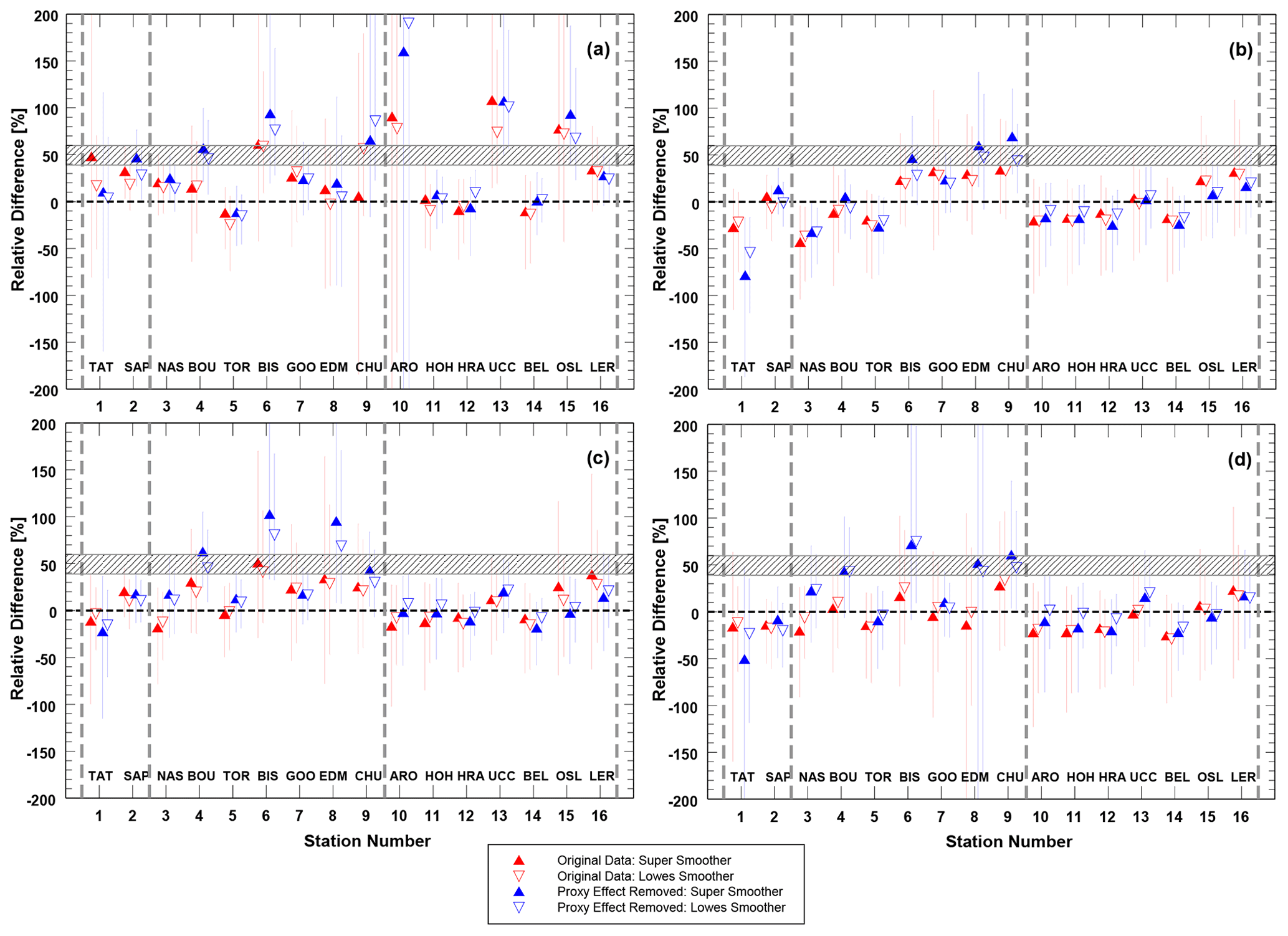
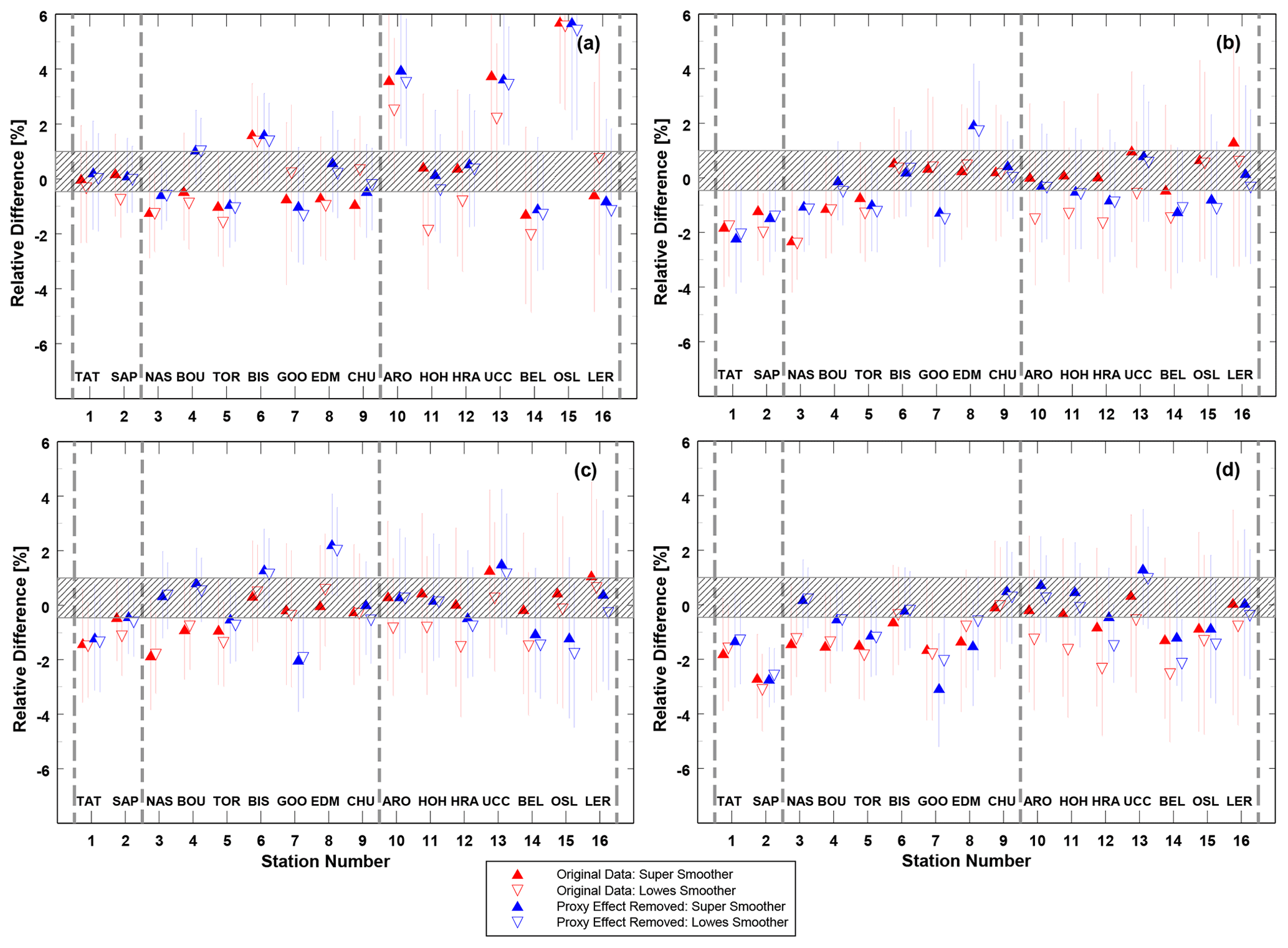
Figure A3The same as Fig. A1 but for ORI1(1988,2020) based on the TCO3 monthly means averaged over the cold sub-period of the year (October–next year March).
The TCO3 data used in this study are taken from the WEB sources, listed in Table 2, with non-limited access. “Full model” version of MLR by Weber at al. (2022) is applied to remove “natural” variability from the original TCO3 data. The MLR proxy set is taken from the WEB sources listed in their Table 2.
The contact author has declared that neither of the authors has any competing interests.
Publisher’s note: Copernicus Publications remains neutral with regard to jurisdictional claims in published maps and institutional affiliations.
This article is part of the special issue “Atmospheric ozone and related species in the early 2020s: latest results and trends (ACP/AMT inter-journal SI)”. It is not associated with a conference.
We thank the Chief Inspectorate of Environmental Protection, Poland, for funding the ozone measurements at Belsk.
This work was supported by the Ministry of Science and Higher Education of Poland under grant number 3841/E-41/S/2022.
This paper was edited by Jens-Uwe Grooß and reviewed by two anonymous referees.
Arosio, C., Rozanov, A., Malinina, E., Weber, M., and Burrows, J. P.: Merging of ozone profiles from SCIAMACHY, OMPS and SAGE II observations to study stratospheric ozone changes, Atmos. Meas. Tech., 12, 2423–2444, https://doi.org/10.5194/amt-12-2423-2019, 2019.
Ball, W. T., Alsing, J., Mortlock, D. J., Staehelin, J., Haigh, J. D., Peter, T., Tummon, F., Stübi, R., Stenke, A., Anderson, J., Bourassa, A., Davis, S. M., Degenstein, D., Frith, S., Froidevaux, L., Roth, C., Sofieva, V., Wang, R., Wild, J., Yu, P., Ziemke, J. R., and Rozanov, E. V.: Evidence for a continuous decline in lower stratospheric ozone offsetting ozone layer recovery, Atmos. Chem. Phys., 18, 1379–1394, https://doi.org/10.5194/acp-18-1379-2018, 2018.
Barnes, P. W., Williamson, C. E., Lucas, R. M, Robinson, S. A., Madronich, S., Paul, N. D., Bornman, J. F., Bais, A. F., Sulzberger, B., Wilson, S. R., Andrady, A. L., McKenzie, R. L., Neale, P. J., Austin, A.T., Bernhard, G. H., Solomon, K. R., Neale, R. E., Young, P. J., Norval, M., Rhodes, L. E., Hylander, S., Rose, K. C., Longstreth, J., Aucamp, P. J., Ballaré, C. L., Cory, R. M., Flint, S. D., de Gruijl, F. R., Häder, D., Heikkilä, A. M., Jansen, M. A., Pandey, K. K., Robson, T. M., Sinclair, C. A., Wängberg, S., Worrest, R. C., Yazar, S., Young, A. R., and Zepp, R. G.: Ozone depletion, ultraviolet radiation, climate change and prospects for a sustainable future, Nat Sustain., 2, 569–579, https://doi.org/10.1038/s41893-019-0314-2, 2019.
Bozhkova, V., Liudchik, A., and Umreiko, S.: Long-term trends of total ozone content over mid-latitudes of the Northern Hemisphere, Int. J. Remote Sens., 40, 5216–5229, https://doi.org/10.1080/01431161.2019.1579384, 2019.
Chubachi, S.: Preliminary results of ozone observations at Syowa Station from February 1982 to January 1983, in: Proc. Sixth Symposium on Polar Meteorology and Glaciology, edited by: Kusunoki, K., Vol. 34 of Mem. National Institute of Polar Research Special Issue, 13–19, 1984.
Cleveland, W. S.: Robust locally weighted regression and smoothing scatterplots, J. Am. Stat. Assoc., 74, 829–836, https://doi.org/10.2307/2286407, 1979.
Coldewey-Egbers, M., Loyola, D. G., Lerot, C., and Van Roozendael, M.: Global, regional and seasonal analysis of total ozone trends derived from the 1995–2020 GTO-ECV climate data record, Atmos. Chem. Phys., 22, 6861–6878, https://doi.org/10.5194/acp-22-6861-2022, 2022.
Delage, O., Portafaix, T., Bencherif, H., Bourdier, A., and Lagracie, E.: Empirical adaptive wavelet decomposition (EAWD): an adaptive decomposition for the variability analysis of observation time series in atmospheric science, Nonlin. Processes Geophys., 29, 265–277, https://doi.org/10.5194/npg-29-265-2022, 2022.
Dietmüller, S., Garny, H., Eichinger, R., and Ball, W. T.: Analysis of recent lower-stratospheric ozone trends in chemistry climate models, Atmos. Chem. Phys., 21, 6811–6837, https://doi.org/10.5194/acp-21-6811-2021, 2021.
Farman, J. C., Gardiner, B. G., and Shanklin, J. D.: Large losses of total ozone in Antarctica reveal seasonal ClOx/NOx interaction, Nature, 315, 207–210, https://doi.org/10.1038/315207a0, 1985.
Friedman, J. H.: A variable span smoother. Laboratory for Computational Statistics, Department of Statistics, Stanford University: Technical Report, SLAC-PUB-3477, https://doi.org/10.2172/1447470, 1984.
Frith, S. M., Kramarova, N. A., Stolarski, R. S., McPeters, R.D., Bhartia, P. K., and Labow, G. J.: Recent changes in total column ozone based on the SBUV Version 8.6 Merged Ozone Data Set, J. Geophys. Res.-Atmos., 119, 9735–9751, https://doi.org/10.1002/2014JD021889, 2014.
Harris, N. R. P., Kyrö, E., Staehelin, J., Brunner, D., Andersen, S.-B., Godin-Beekmann, S., Dhomse, S., Hadjinicolaou, P., Hansen, G., Isaksen, I., Jrrar, A., Karpetchko, A., Kivi, R., Knudsen, B., Krizan, P., Lastovicka, J., Maeder, J., Orsolini, Y., Pyle, J. A., Rex, M., Vanicek, K., Weber, M., Wohltmann, I., Zanis, P., and Zerefos, C.: Ozone trends at northern mid- and high latitudes – a European perspective, Ann. Geophys., 26, 1207–1220, https://doi.org/10.5194/angeo-26-1207-2008, 2008.
Hudson, R. D., Andrade, M. F., Follette, M. B., and Frolov, A. D.: The total ozone field separated into meteorological regimes – Part II: Northern Hemisphere mid-latitude total ozone trends, Atmos. Chem. Phys., 6, 5183–5191, https://doi.org/10.5194/acp-6-5183-2006, 2006.
Komhyr, W. D.: Dobson spectrophotometer systematic total ozone measurement error, Geophys. Res. Lett., 7, 161–163, https://doi.org/10.1029/GL007i002p00161, 1980.
Krzyścin, J. W. and Rajewska-Więch, B.: Specific variability of total ozone over Central Europe during spring and summer in the period 1979–2014, Int. J. Clim., 36, 3539–3549, https://doi.org/10.1002/joc.4574, 2016.
Krzyścin, J. W., Rajewska-Więch, B., and Pawlak, I.: Long-Term Ozone Changes Over the Northern Hemisphere Mid-Latitudes for the 1979–2012 Period, Atmos. Ocean, 53, 153–160, https://doi.org/10.1080/07055900.2014.990869, 2015.
Laine, M., Latva-Pukkila, N., and Kyrölä, E.: Analysing time-varying trends in stratospheric ozone time series using the state space approach, Atmos. Chem. Phys., 14, 9707–9725, https://doi.org/10.5194/acp-14-9707-2014, 2014.
Laube, J. C., Engel, A., Bönisch, H., Möbius, T., Sturges, W. T., Braß, M., and Röckmann, T.: Fractional release factors of long-lived halogenated organic compounds in the tropical stratosphere, Atmos. Chem. Phys., 10, 1093–1103, https://doi.org/10.5194/acp-10-1093-2010, 2010.
Mäder, J. A., Staehelin, J., Brunner, D., Stahel, W. A., Wohltmann, I., and Peter, T.: Statistical modeling of total ozone: Selection of appropriate explanatory variables, J. Geophys. Res., 112, D11108, https://doi.org/10.1029/2006JD007694, 2007.
Maillard Barras, E., Haefele, A., Stübi, R., Jouberton, A., Schill, H., Petropavlovskikh, I., Miyagawa, K., Stanek, M., and Froidevaux, L.: Dynamical linear modeling estimates of long-term ozone trends from homogenized Dobson Umkehr profiles at Arosa/Davos, Switzerland, Atmos. Chem. Phys., 22, 14283–14302, https://doi.org/10.5194/acp-22-14283-2022, 2022.
Montzka, S. A., Dutton, G., and Vimont, I.: The NOAA Ozone Depleting Gas Index: Guiding Recovery of the Ozone Layer, https://gml.noaa.gov/odgi/ (last access: 27 February 2023), 2022.
Newman, P. A., Nash, E. R., Kawa, S. R., Montzka, S. A., and Schauffler, S. M.: When will the Antarctic ozone hole recover?, Geophys. Res. Lett., 33, L12814, https://doi.org/10.1029/2005GL025232, 2006.
Reinsel, G. C., Miller, A. J., Weatherhead, E. C., Flynn, L. E., Nagatani, R. M., Tiao, G. C., and Wuebbles, D. J.: Trend analysis of total ozone data for turnaround and dynamical contributions, J. Geophys. Res., 110, D16306, https://doi.org/10.1029/2004JD004662, 2005.
Sato, M., Hansen, J. E., McCormick, M. P., and Pollack, J. B.: Stratospheric aerosol optical depths, 1850–1990, J. Geophys. Res., 98, 22987–22994, https://doi.org/10.1029/93JD02553, 1993.
Solomon, S., Garcia, R. R., Rowland, F. S., and Wuebbles, D. J.: On the depletion of Antarctic ozone, Nature, 321, 755–758, https://doi.org/10.1038/321755a0, 1986.
Szela̧g, M. E., Sofieva, V. F., Degenstein, D., Roth, C., Davis, S., and Froidevaux, L.: Seasonal stratospheric ozone trends over 2000–2018 derived from several merged data sets, Atmos. Chem. Phys., 20, 7035–7047, https://doi.org/10.5194/acp-20-7035-2020, 2020.
Thompson, A. M., Stauffer, R. M., Wargan, K., Witte, J. C., Kollonige, D. E., and Ziemke, J. R.: Regional and seasonal trends in tropical ozone from SHADOZ profiles: Reference for models and satellite products, J. Geophys. Res.-Atmos., 126, e2021JD034691, https://doi.org/10.1029/2021JD034691, 2021.
van der A, R. J., Allaart, M. A. F., and Eskes, H. J.: Extended and refined multi sensor reanalysis of total ozone for the period 1970–2012, Atmos. Meas. Tech., 8, 3021–3035, https://doi.org/10.5194/amt-8-3021-2015, 2015.
Velders, G. J. M. and Daniel, J. S.: Uncertainty analysis of projections of ozone-depleting substances: mixing ratios, EESC, ODPs, and GWPs, Atmos. Chem. Phys., 14, 2757–2776, https://doi.org/10.5194/acp-14-2757-2014, 2014.
Wald, A. and Wolfowitz, J.: On a test whether two samples are from the same population, Ann. Math. Stat., 11, 147–162, https://doi.org/10.1214/aoms/1177731909, 1940.
Wargan, K., Labow, G. J., Frith, S. M., Pawson, S., Livesey, N. J., and Partyka, G. S.: Evaluation of the Ozone Fields in NASA's MERRA-2 Reanalysis., J. Climate, 30, 2961–2988, https://doi.org/10.1175/JCLI-D-16-0699.1, 2017.
Weber, M., Coldewey-Egbers, M., Fioletov, V. E., Frith, S. M., Wild, J. D., Burrows, J. P., Long, C. S., and Loyola, D.: Total ozone trends from 1979 to 2016 derived from five merged observational datasets – the emergence into ozone recovery, Atmos. Chem. Phys., 18, 2097–2117, https://doi.org/10.5194/acp-18-2097-2018, 2018.
Weber, M., Arosio, C., Coldewey-Egbers, M., Fioletov, V. E., Frith, S. M., Wild, J. D., Tourpali, K., Burrows, J. P., and Loyola, D.: Global total ozone recovery trends attributed to ozone-depleting substance (ODS) changes derived from five merged ozone datasets, Atmos. Chem. Phys., 22, 6843–6859, https://doi.org/10.5194/acp-22-6843-2022, 2022.
WMO: Scientific Assessment of Ozone Depletion: 1998, Global Ozone Research and Monitoring Project – Rep. No. 44, World Meteorological Organization, Geneva, Switzerland, 496 pp., 1999.
WMO: Executive Summary. Scientific Assessment of Ozone Depletion: 2022, GAW Report No. 278, World Meteorological Organization, Geneva, Switzerland, 56 pp., 2022.