the Creative Commons Attribution 4.0 License.
the Creative Commons Attribution 4.0 License.
 | 27 Feb 2023
O3–precursor relationship over multiple patterns of timescale: a case study in Zibo, Shandong Province, China
Zhensen Zheng
Kangwei Li
Bo Xu
Jianping Dou
Liming Li
Guotao Zhang
Shijie Li
Chunmei Geng
Wen Yang
Merched Azzi
Zhipeng Bai
In this study, we developed an approach that integrated multiple patterns of timescale for box modeling (MCMv3.3.1) to better understand the O3–precursor relationship at multiple sites and through continuous observations. A 5-month field campaign was conducted in the summer of 2019 to investigate the ozone formation chemistry at three sites in a major prefecture-level city (Zibo) in Shandong Province of northern China. It was found that the relative incremental reactivity (RIR) of major precursor groups (e.g., anthropogenic volatile organic compounds (AVOCs), NOx) was overall consistent in terms of timescales changed from wider to narrower (four patterns: 5-month, monthly, weekly, and daily) at each site, though the magnitudes of RIR varied at different sites. The time series of the photochemical regime (using RIR RIRAVOC as an indicator) in weekly or daily patterns further showed a synchronous temporal trend among the three sites, while the magnitude of RIR RIRAVOC was site-to-site dependent. The derived RIR ranking (top 10) of individual AVOC species showed consistency between three patterns (i.e., 5-month, monthly, and weekly). It was further found that the campaign-averaging photochemical regimes showed overall consistency in the sign but non-negligible variability among the four patterns of timescale, which was mainly due to the embedded uncertainty in the model input dataset when averaging individual daily patterns into different timescales. This implies that utilizing narrower timescales (i.e., daily pattern) is useful for deriving reliable and robust O3–precursor relationships. Our results highlight the importance of quantifying the impact of different timescales to constrain the photochemical regime, which can formulate more accurate policy-relevant guidance for O3 pollution control.
- Article
(4304 KB) - Full-text XML
-
Supplement
(4635 KB) - BibTeX
- EndNote


Since 2013, the ambient PM2.5 concentration in China has dramatically declined following the implementation of the Clean Air Action (Lu et al., 2018; Y. Wang et al., 2020; Zhang et al., 2019). However, national ground surface ozone concentrations increased over the same period (Xue et al., 2020) and became a major air quality problem that needed to be addressed in China (Li et al., 2019; Wang et al., 2019). It is well-known that ground surface ozone is formed mainly by complex nonlinear photochemical oxidation of volatile organic compounds (VOCs) in the presence of nitrogen oxides (NOx= NO + NO2) and sunlight (Blanchard, 2000; Hidy, 2000; Kleinman, 2000), which adversely influences human health, vegetation, and crops (Brunekreef and Holgate, 2002; Vingarzan, 2004).
Given the complex non-linear relationship between O3 formation and its precursors (VOCs and NOx), challenges in mitigating its severity lie primarily in comprehensively understanding the O3–precursor relationship (Su et al., 2018a; Tan et al., 2018a). It is commonly recognized that regional-scale air quality models and the 0-D box model are two mainstream approaches to investigate the increasingly severe ozone problem (Blanchard, 2000; Cardelino and Chameides, 1995; Hidy, 2000; Liu et al., 2019). Unlike the complicated 3-D air quality models, the 0-D box model is an observation-based model that is implemented with a gas-phase chemical mechanism; it has been widely used to diagnose O3–precursor relationships in various locations (Liu et al., 2021a; Sun et al., 2016; Tan et al., 2019; Xue et al., 2014a; Yu et al., 2020a). Some previous studies (Li et al., 2021; Lu et al., 2010a; Sicard et al., 2020; Yu et al., 2020b) have reported large variability in O3–precursor relationships on spatiotemporal scales in many cities of China, which indicates great challenges for current O3 pollution control (Y. Wang et al., 2017; Xue et al., 2014b).
Table 1 summarizes the published studies of O3–precursor relationships using the 0-D box model (implemented with different gas-phase chemical mechanisms) with diversified patterns of timescale in many places in China. The observational period in most previous studies was short term (i.e., less than one month), while medium-term (i.e., from one to several months), and long-term (i.e., multiple years) periods were limited. As shown in Table 1, we find that model input datasets with different timescales have been employed in previous studies to identify the campaign-averaging O3 formation regime, but there is a lack of comparison among these different timescales. We also find that more than half of the studies use the averaged diurnal patterns as box model input, which is particularly common for medium- and long-term measurements. For example, a 10-year long-term observational study by Y. Wang et al. (2017) adopted a monthly pattern of timescale for model simulation for the reason of saving computing resources; it also revealed a substantial temporal variability in the O3–precursor relationship. In addition, it is believed that long-term (measurements of at least several months) and multiple-site continuous online measurements can provide an opportunity to develop O3 control strategies more comprehensively over a wider spatiotemporal scale (Li et al., 2021; Y. Wang et al., 2017; T. Wang et al., 2017). However, such measurements have been quite rare in China, limiting the present understanding of O3–precursor relationships (Lu et al., 2019; T. Wang et al., 2017).
Table 1Summary of relevant published 0-D box model studies in China.
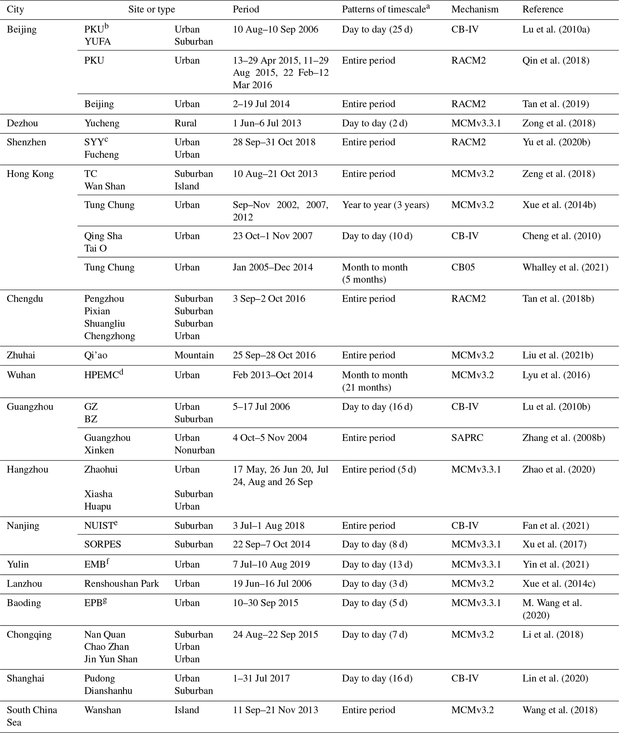
a Number of days for modeling the patterns of timescale denotes that which was simulated by the box model. b Peking University. c Shenzhen Yanjiusheng Yuan. d Hubei Provincial Environmental Monitoring Center. e Nanjing University of Information Science & Technology. f Environmental Monitoring Building. g Environmental Protection Bureau.
In this study, a 5-month field campaign was conducted in the summer of 2019 to investigate the ozone formation chemistry at three sites in Zibo, a major prefecture-level Chinese city in Shandong Province. According to our measurements at the three sites in Zibo, the averaged O3 concentration during the whole observational period was around 50 ppbv, while the daily maximum of O3 concentrations for some extremely polluted periods were nearly 120–150 ppbv (see details in Sect. 3.1). Here, we developed an approach that integrated multiple patterns of timescale for box model simulation, which aimed to illustrate the non-linearity of O3–precursor relationships driven by their actual daily, weekly, and monthly variability. Our results can be conducive to interpreting variations of O3–precursor relationships over a wider spatiotemporal scale, and they provide implications for developing more precise and constrained O3 control strategies in other regions.
2.1 Study sites and measurements
Field measurements were conducted in a major prefecture-level city (Zibo), which is in the middle of Shandong Province, northern China, from 1 May to 30 September 2019. Figure S1 in the Supplement shows the surrounding environment and geographical locations at the three sampling sites; a detailed description of the Tianzhen (TZ), Beijiao (BJ), and Xindian (XD) sites can be found in our previous study (Li et al., 2021). Briefly, TZ contains a mixture of crude oil processing and operation stations and farming areas and is classified as a suburban area; XD contains a mixture of residential and heavy industrial zones and is considered to be a suburban area; BJ is in the urban area of Zibo.
Typical inorganic gases of O3, NO, NO2, CO, and SO2 were measured using online commercial gas analyzers (Thermo Scientific 49i, 42i, 48i, and 43i, USA) at the three sites. Following the Chinese meteorological monitoring regulation (GB/T 35221-2017), we continuously monitored the meteorological parameters (i.e., temperature, relative humidity, UV-A solar radiation, precipitation, wind speed, and wind direction) at the three sites (Li et al., 2021). Two online GC systems (gas chromatography–flame ionization detector, GC–FID, Thermo Scientific GC5900) were deployed at TZ and BJ respectively to measure VOC species. For C2-C5 VOCs, desorption and separation were performed using a GC with pre-concentration on a combination of two columns, followed by an FID detector. For C6-C12 VOCs, the air sample was pre-concentrated on Tenax GR cartridges and subsequently separated by chromatographic column, then it was detected by another FID detector. Similarly, one online system (gas chromatography–flame ionization detector–photoionization detector, GC–FID–PID, Syntech Spectras GC 955-615/815) was deployed at the XD site. For C2-C6 VOCs, the hydrocarbons were concentrated on a Tenax GR carrier then thermally desorbed and separated on a DB-1 column before finally being detected by the FID and PID. For C6-C12 VOCs, the air sample was concentrated on a Carbosieve SIII carrier at 5∘ then thermally desorbed and separated on a combination of two columns; the FID and PID detectors were employed for subsequent detection. These systems measured 55 VOC species at a 1 h resolution; more detailed descriptions can be found elsewhere (Chien, 2007; Jiang et al., 2018; Xie et al., 2008).
Table S1 summarized the limit of detection, accuracy, and precision of the instruments at the three sites, and all the measurement instruments were regularly subjected to service checking and maintenance during the whole campaign. Unfortunately, we did not conduct the inter-comparison between the GC–FID and GC–FID–PID instruments at the same site due to practical reasons, as these VOC instruments were separately deployed at the three different sites for continuous routine operation. To ensure the quality assurance and quantity control (QA–QC) of online VOC measurement, two five-point calibrations (i.e., 2, 4, 6, 8, 10 ppbv, dilution from one cylinder) for standard gases with 55 VOC species (Linde Co., Ltd, USA) were carried out in May and August of 2019 at the three sites. Table S2 showed that the calibration linearity (R2) of all measured VOCs was nearly 0.9990. Additionally, a single-point calibration (i.e., 6 ppbv) was regularly performed every month during the whole campaign. As shown in Fig. S2 (a case from TZ), the retention time, peak fitting, and baseline of the chromatogram were manually checked and adjusted on a daily basis.
2.2 0-D box model and design of four patterns of timescale
The 0-D box model integrated with the latest Master Chemical Mechanism MCMv3.3.1 (http://mcm.york.ac.uk, last access: 27 January 2023) has been widely utilized in many regions (He et al., 2019; Jenkin et al., 2015; Liu et al., 2019; Whalley et al., 2021). Unlike the lumped chemical mechanisms such as CB05 (Y. Wang et al., 2017; Yarwood et al., 2005), CB6 (Yarwood et al., 2010), RACM and RACM2 (Goliff et al., 2013; Stockwell et al., 1997, 2020), and SAPRC-07 (Carter, 2010), the MCMv3.3.1 is a near-explicit chemical mechanism consisting of over 5800 species and 17 000 reactions (Jenkin et al., 2015; Saunders et al., 2003), which can be used to describe the gas-phase chemistry (i.e., in situ photochemistry). In this study, the box model (based on the Framework for 0-D Atmospheric Modeling, F0AM; Wolfe et al., 2016) was applied and constrained by the mean diurnal profiles of meteorological data (i.e., temperature, relative humidity, and photolysis rates), 4 inorganic gases (i.e., SO2, CO, NO, and NO2), and 45 speciated VOCs (in MCMv3.3.1 species list; see Table S3). Since measured photolysis rates (J values) were not available, the measured UV-A solar radiation was used to scale the photolysis rates calculated from the Tropospheric Ultraviolet and Visible Radiation model (TUVv5.2; https://www.acom.ucar.edu/Models/TUV/Interactive_TUV; last access: 27 January 2023) following the approach of recent studies (Lyu et al., 2019, 2016). Specifically, the geographical coordinates, date, and time were initialized into the TUV model to derive photolysis rates and solar radiation. We obtained the scaling factor by comparing the observed with modeled solar radiation and used this scaling factor to scale the TUV-model-derived photolysis rates. A dilution rate of s−1 was applied for all non-constraint species and simulation days through a stepwise sensitivity test by adjusting it from to s−1 (see details in Sect. S1) for the best reproduction of O3. For each model run (i.e., each daily model simulation), it was performed on a daily basis with intervals of 24 h spanning from 00:00 to 23:00 LT (local time), and each individual model simulation was run to reach one-day diurnal steady state. The detailed descriptions of box model operation were provided in our previous study (Li et al., 2021).
Since the box model simulations are conducted with intervals of 24 h spanning from 00:00 to 23:00 LT (Wang et al., 2018), the entire campaign's observations were classified into four patterns of timescale (i.e., 5-month, monthly, weekly, and daily) as diurnal-average formats for model input (Fig. 1). Note that some days or weeks were not modeled due to some missing data in the measurements. Nevertheless, the total simulation number at the daily (i.e., 100, 81, and 114 d for TZ, BJ, and XD respectively) or weekly (i.e., 21, 20, and 19 weeks for TZ, BJ, and XD respectively) scale was representative of the 5-month campaign. Specifically, the entire campaign data classified as four patterns of timescale were modeled as base runs. Then we performed the sensitivity modeling to calculate the relative incremental reactivity (RIR) of precursors by adjusting the input concentrations in the base runs (see next section) (Lu et al., 2010a).
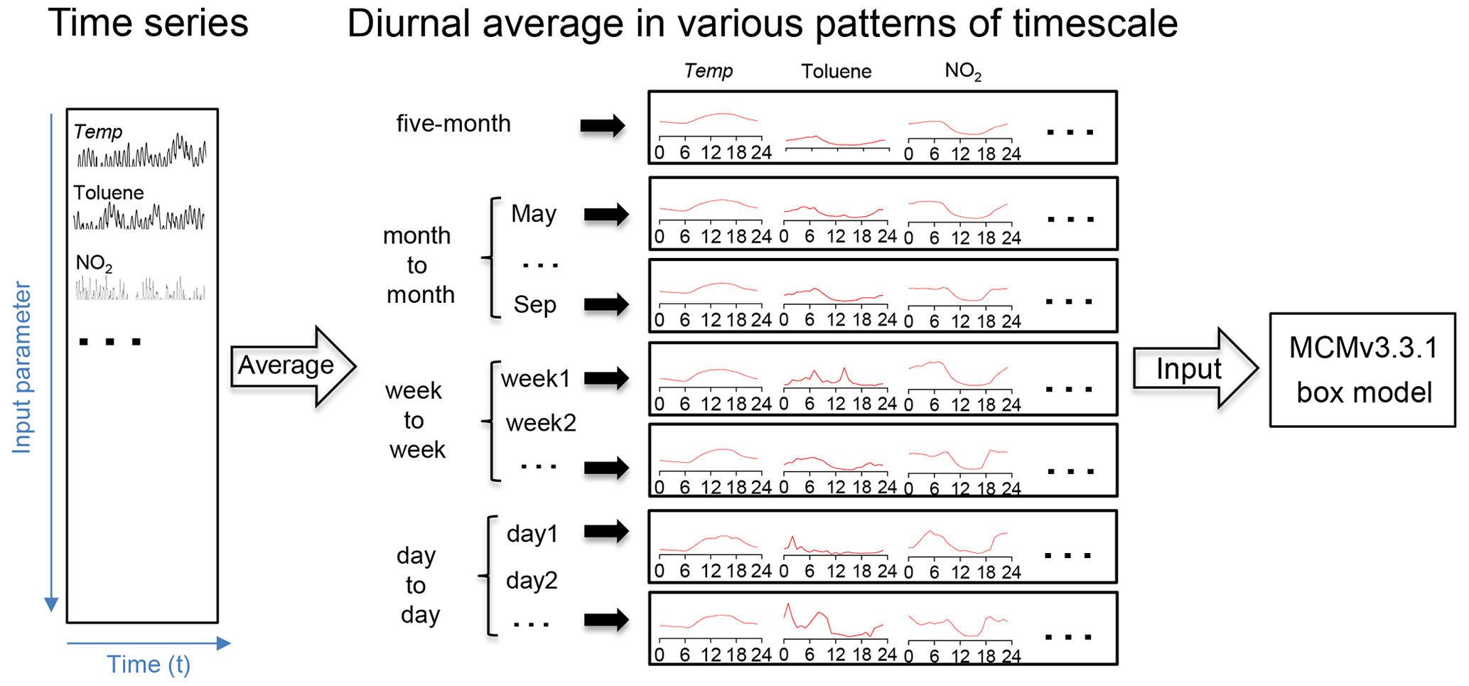
Figure 1Schematic diagram of the dataset treatment to derive four patterns of timescale for 0-D box model input. Note that the four patterns (i.e., 5-month, monthly, weekly, and daily) were the diurnal average of the initial dataset. This diagram takes one site and several input measurements (temperature, toluene, and NO2) as examples.
2.3 Calculation of net Ox production rate P(Ox) and relative incremental reactivity (RIR)
Considering the rapid chemical titration of NO to NO2 in the presence of O3, the concept of “total oxidant” (Ox= O3+ NO2) has been widely used to represent the actual photochemical production of O3 (Lu et al., 2010a). Similar to those described in previous studies using the 0-D box model (He et al., 2019; Lyu et al., 2016), the net or in situ Ox production rate (P(Ox)) is defined as the difference between the Ox gross production rate (G(Ox)) and the Ox destruction rate (D(Ox)), which is formulated in accordance with Eq. (1):
The Ox gross production rate (G(Ox)), or the total chemical production of Ox, is calculated by summing the rates of oxidation of NO by HO2 and RO2 radicals in accordance with Eq. (2):
The Ox destruction rate (D(Ox)), or total chemical loss of Ox, is calculated by summing O3 photolysis, the reaction of O3 with OH, HO2, and alkenes, and the reaction between NO2 and OH, as described by Eq. (3):
Concentrations of radicals and intermediates are obtained from the outputs of the 0-D box model. The k values in Eqs. (2) and (3) represent the rate constants of the corresponding reactions, respectively. The subscript “i” in Eq. (2) represents the individual RO2 species.
Additionally, relative incremental reactivity (RIR) has been widely used as a metric to quantify the O3–precursor relationship, and it can be derived from the 0-D box model (MCMv3.3.1) by changing the input mixing ratios of its precursors (Sillman, 2010; Xue et al., 2014a). The RIR is defined as the ratio of percentage change in net Ox (Ox= O3+ NO2) production rate P(Ox) (Li et al., 2021) to the percentage change of the concentration of precursor X. The RIR of a specific precursor X is described in Eq. (4):
Here, X is a specific precursor (i.e., NOx, CO, or grouped or individual VOC species), CX is the measured concentration of precursor X, and ΔCX is the hypothetical concentration change (ΔCX CX = 10 % in this study in accordance with the previous studies (Lyu et al., 2016; Wang et al., 2018)). POx(CX) represents the simulated Ox production rate in a base run, whereas POx(CX–ΔCX) is the simulated Ox production in a second run with a hypothetical concentration change of species X. Obviously, a higher positive value of RIR(X) suggests a more effective way of reducing the ambient O3 production rate by reducing X (Ling et al., 2011; Zhang et al., 2008a).
In this study, the O3 precursors were divided into four major categories, including anthropogenic VOCs (AVOCs), biogenic VOCs (BVOCs, only isoprene in this study), CO, and NOx (Tan et al., 2019). AVOCs were further divided into three subcategories: alkanes, aromatics, and alkenes* (the asterisk denotes anthropogenic alkenes, excluding isoprene in this study; Yu et al., 2020a). As mentioned, RIR method was applied mainly to evaluate the O3–NOx–VOC sensitivity and to determine the photochemical regimes among four patterns of timescale. Thus, we calculated the RIR values of major precursor groups (i.e., AVOCs, BVOCs, CO, NOx, alkanes, alkenes*, and aromatics) to further quantify the O3–precursor relationship.
In general, O3 formation chemistry is usually classified into three regimes (i.e., VOC-limited, transitional, and NOx-limited; He et al., 2019; Wang et al., 2018). In this study, RIR RIRAVOC (the ratio of two RIR values) was used as a metric to classify the photochemical regimes (Li et al., 2021). Specifically, a RIR RIRAVOC value of less than 0.5 was defined as a VOC-limited regime; a value greater than 2 was defined as a NOx-limited regime; and a value from 0.5 to 2 was defined as a transitional regime (see Sect. S2 and Table S4) (Li et al., 2021).
3.1 Overview of the field campaign
Figure 2 shows the time series of measured meteorological parameters and O3, as well as its precursors at the three sites during the whole campaign. In general, the temperature (T) and relative humidity (RH) were basically consistent at the three sites, while the wind speeds were different, which suggests that the three sites had an overall consistent meteorological condition. In addition, the time series of UV-A radiation was shown in Fig. 2d, which was only available from one urban site of Zibo but was expected to represent the whole Zibo city in this study. Following the protocol of the previous studies (Lyu et al., 2019; Y. Wang et al., 2017; Xue et al., 2014c), the time series of photolysis rates (e.g., (Fig. 2e) and (Fig. 2f)) were calculated from TUVv5.2 model and further scaled from UV-A radiation measurement.
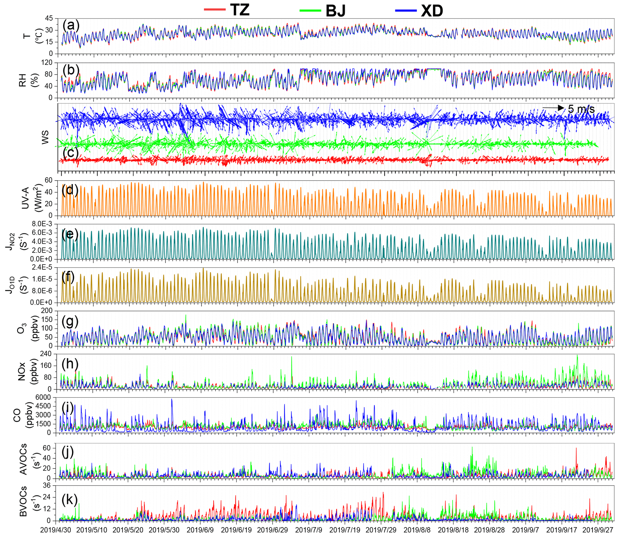
Figure 2Time series of meteorological parameters, O3, and its precursors (i.e., CO, NOx, VOCs) throughout the whole campaign at the three sites in Zibo.
As shown in Fig. 2g, we found that severe O3 pollution was observed at the three sites throughout the whole campaign. According to our measurements at the three sites in Zibo, the averaged O3 concentration during the whole observational period was around 50 ppbv, while the daily maximum of O3 concentrations for some extremely polluted periods were nearly 120–150 ppbv (Fig. 2g). Interestingly, the O3 concentrations at the three sites were generally consistent, while the levels of its precursors (e.g., VOCs, NOx) were obviously different (Fig. 2h–k), which implies the site-to-site variation of O3 formation chemistry for the whole city of Zibo.
Generally, OH reactivity (or OH loss rate, kOH) is widely applied to quantify the capacity of OH consumption by VOCs (Tan et al., 2019). According to Table S3, the BVOC reactivity (kBVOC, 3.5±4.1 s−1) in TZ was highest among the three sites. As BJ was mainly influenced by the emission from urban region, it showed the highest AVOC reactivity (kAVOC, 6.8±6.3 s−1) and NOx level (31.1±28.6 ppbv). In addition, XD showed the highest level of alkenes* reactivity of 4.0±3.2 s−1 within the three sites, and the local petrochemical industry nearby the XD area may explain such a characteristic (Li et al., 2021).
3.2 Evaluation of box model performance
The measured O3 concentrations were not constrained in our MCMv3.3.1 box model calculation; thus the model performance could be quantitatively assessed by comparing the modeled O3 (from base runs) with the measured O3. Figures S3–S8 show the time series of simulated and observed O3 concentrations at four patterns of timescale. In most cases, the box model simulation could accurately capture the level and variation trend of the observed O3. However, on some days, the modeling results underestimated or overestimated the O3 concentrations – in particular, nocturnal O3 concentrations were underestimated. Such discrepancies between the simulated and observed O3 were likely due to limitations in the explicit representations of atmospheric and transport processes (i.e., the horizontal and vertical transport processes of ground ozone) by the 0-D modeling approach (Lyu et al., 2019; Yu et al., 2020b). Specifically, ozone simulated by the 0-D box model is considered in the same way as in situ photochemical processes from its precursors. Unlike the 3-D air quality model, 0-D box modeling usually simplifies the representation of the physical processes (i.e., deposition and advection; Lu et al., 2010a; Sillman, 2010). Note that some adjustable parameters (e.g., radiation scheme, dilution rate) remained consistent in all of our model calculations, which ensured the comparability of model results to the greatest extent.
The index of agreement (IOA; Li et al., 2021; Lyu et al., 2016), Pearson's correlation coefficient (r), and root-mean-square error (RMSE) were jointly used as statistical metrics to quantify the goodness of fit between the simulated and observed O3 concentrations. Table S5 summarizes these statistical metrics for each site at various patterns of timescale. Because any single statistical metric has its own limitations, using these three indicators conjointly provided a more comprehensive evaluation of the model performance (Su et al., 2018b). Generally, higher IOA and r and lower RMSE indicate better agreement between the simulated and observed values (Wang et al., 2018; Willmott, 1982). As shown in Table S5, slightly reduced correlation was observed as the timescale changed from the wider (i.e., 5-month scale) to the narrower (i.e., daily scale) pattern, which is understandable because of the enlarged statistical samples in the narrower pattern of timescale.
In summary, TZ showed the best performance in terms of the box model simulation, followed by XD and then BJ, regardless of any statistical metrics or different patterns of timescale, which may be associated with the optimized dilution rate for non-constraint species in model configuration. The overall model performance in this study (i.e., a day-to-day IOA of approximately 0.90 for TZ) was close to or slightly better than those reported in previous studies, such as IOA = 0.74 in Hong Kong (Liu et al., 2019), IOA = 0.74 in Wuhan (Lyu et al., 2016), and IOA = 0.90 in Jiangmen (He et al., 2019). According to the above evaluation of base runs, our modeled results were acceptable for the subsequent O3–precursor relationship analysis described in the following sections.
3.3 Month to month
Figure 3a–b presents the monthly RIR values of the major precursor groups at each site, and the large variability of the O3–precursor relationship at a spatiotemporal scale (i.e., site to site and month to month) was observed. Specifically, in most months, XD generally showed the highest RIRAVOC among the three sites, followed by BJ and then TZ. In addition, RIRBVOC showed a similar level to RIRAVOC in TZ but much less than RIRAVOC in BJ and XD, which can be explained by the observed higher BVOC reactivity in TZ than in the other two sites (see Fig. S9 and Table S3). Also, almost all the precursor groups showed positive RIR values, except for the negative RIR that appeared in BJ and XD in September. In addition, the RIRCO values at the three sites suggested its limited role in O3 formation at the three sites compared with other major categories of O3 precursors. Among the three subcategories of AVOCs, alkenes* always had the highest RIR values, followed by aromatics, while the contribution of alkanes to O3 formation can be ignored due to their near-zero RIR values. That sequence of O3–AVOC sensitivity (alkenes* > aromatics > alkanes) indicated by the RIR analysis was consistent with previous studies in some other Chinese cities (Su et al., 2018b; Tan et al., 2019). Significant monthly variations of O3, NOx, CO, VOC reactivity, and TVOC NOx ratios (in ppbC ppbv−1 as a widely used simple metric to determine the photochemical regime; National Research Council, 1991) were also observed from May to September (see Fig. S9 and Table S3) at the three sites. For example, the BVOC reactivity in TZ showed the highest level among the three sites during the whole campaign, and the AVOC reactivity in BJ showed more considerable variations in different months, which indicated spatial and temporal variations of local primary emissions for O3 precursors in the city of Zibo.
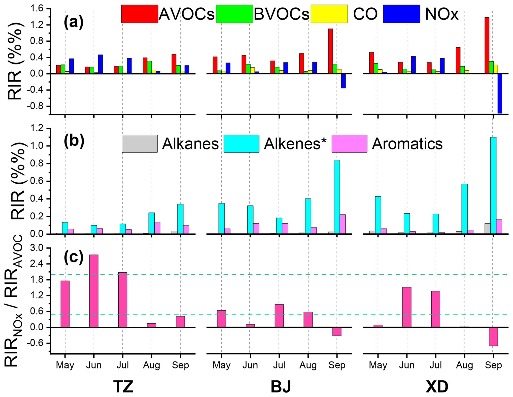
Figure 3Time series of month-to-month RIR values of major precursor groups and RIR RIRAVOC at three sites (TZ, BJ, and XD) in Zibo. The dashed green line indicates RIR RIRAVOC= 0.5 and 2.
Figure 3c shows monthly RIR RIRAVOC at each site, which clearly reveals the spatial and temporal variations in photochemical regimes. For instance, the photochemical regime at the TZ site was considered to be a transitional regime in May, a NOx-limited regime in June and July, and a VOC-limited regime in August and September; on the other hand, for a specific month like June, NOx-limited, VOC-limited, and transitional regimes were generally identified for TZ, BJ, and XD, respectively. Figure 5b shows good consistency between monthly TVOC NOx and RIR RIRAVOC, suggesting that the changes of local emissions for O3 precursors may partially explain the considerable variation of O3 formation chemistry in different months.
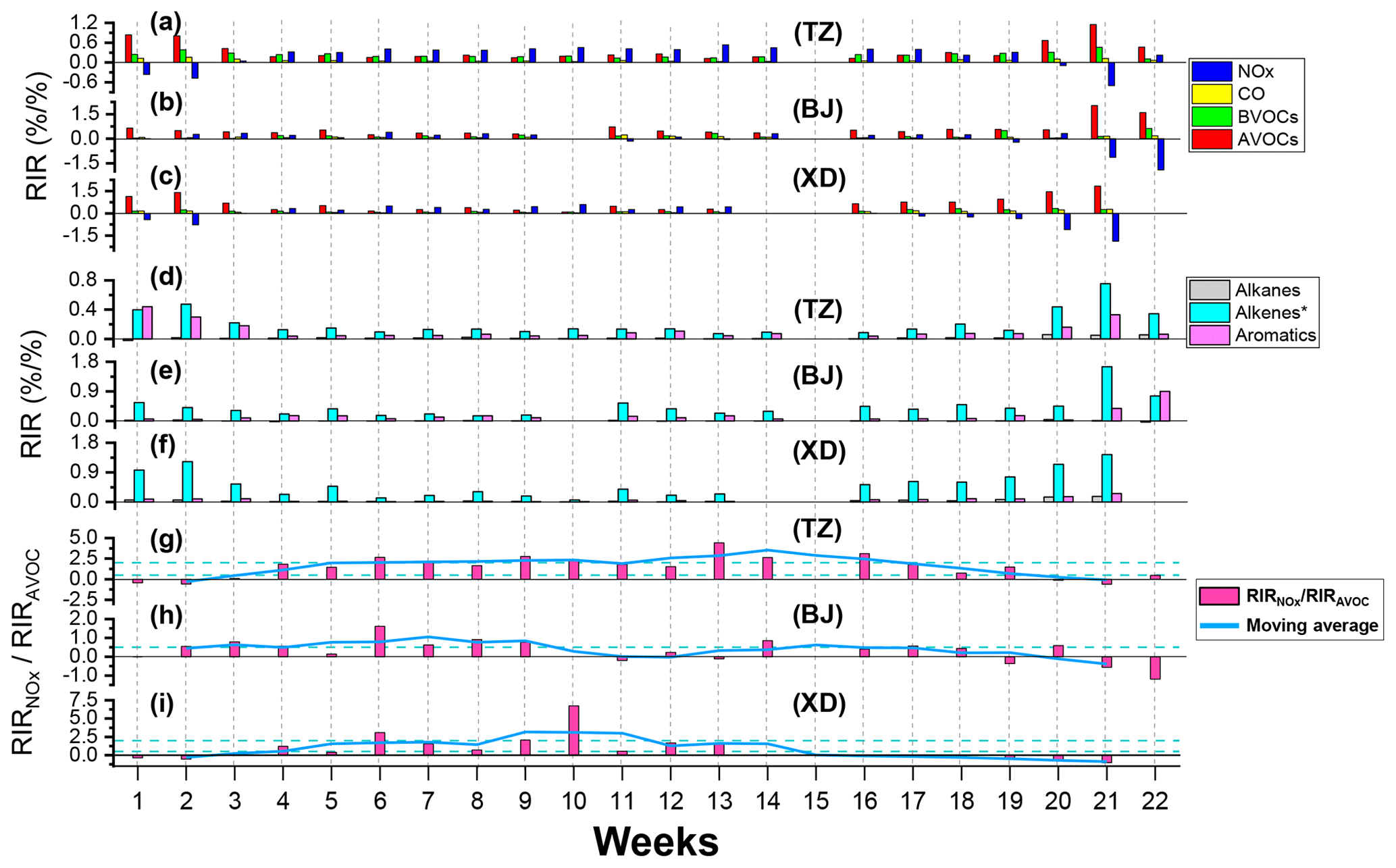
Figure 4Time series of week-to-week RIR values of major precursor groups and RIR RIRAVOC at three sites (TZ, BJ, and XD) in Zibo. The blue lines in (g)–(i) are the three-points moving average of RIR RIRAVOC values.
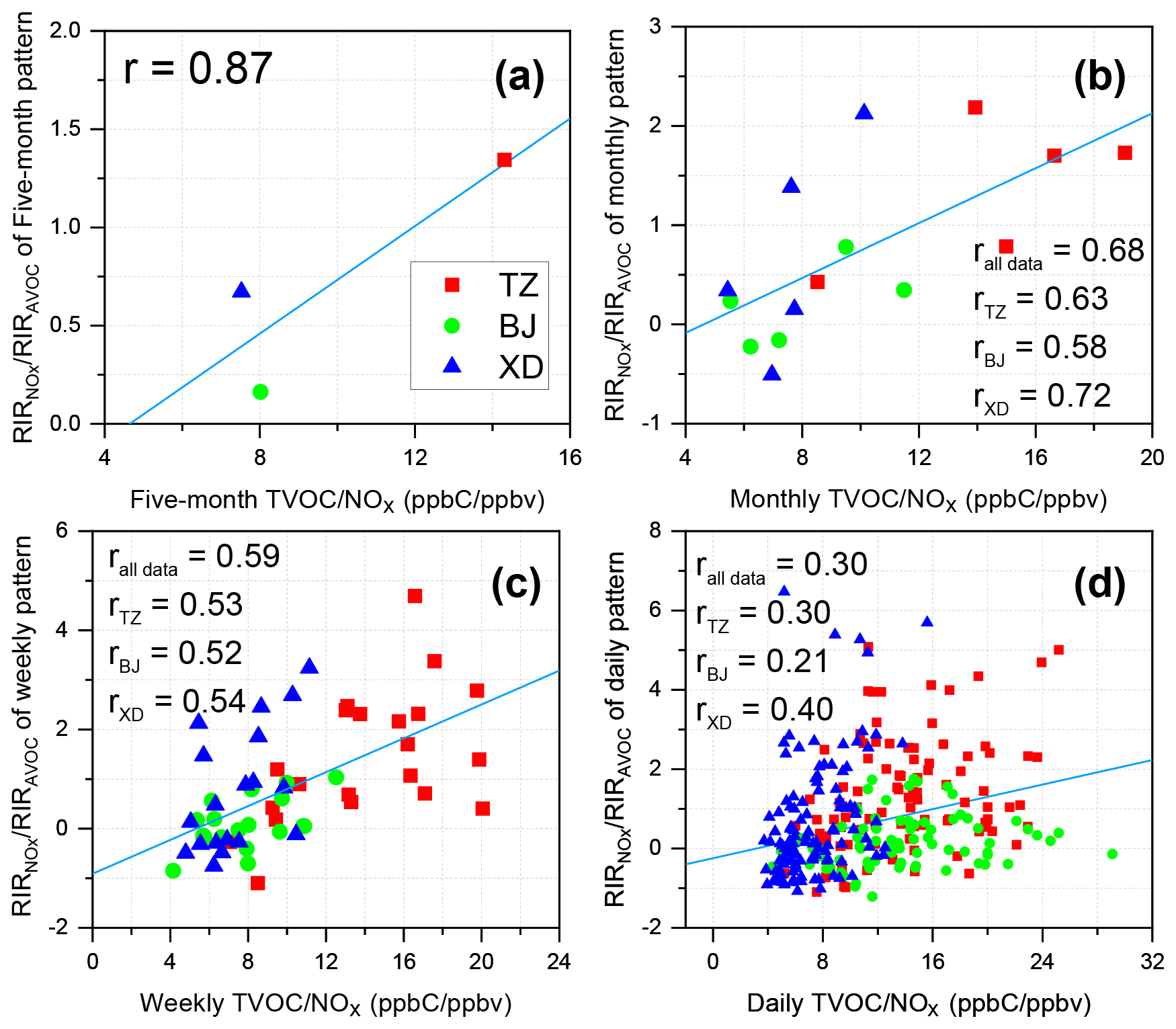
Figure 5The correlations of TVOC NOx with RIR RIRAVOC at multiple patterns of timescale at the three sites in Zibo.
3.4 Week to week
Figure 4 shows the time series of week-to-week RIR values of major precursor groups and RIR RIRAVOC at three sites in Zibo. Compared with month-to-month results, Fig. 4 further reveals the O3–precursor relationship with more information on temporal trends. The temporal variations in weekly RIRAVOC at the three sites generally decreased and then increased, whereas weekly RIR represented an opposite temporal variation during the entire campaign. Additionally, weekly RIRBVOC showed a trend of first decreasing and then increasing at TZ, while it did not show clear temporal variations at BJ and XD due to low values (Fig. 4a–c). In general, RIRalkanes, RIR, and RIRaromatics showed a tendency consistent with that of the RIRAVOC at the three sites (Fig. 4d–f). Overall, these phenomena were consistent among the three sites, though the magnitude of RIR values varied site to site. In parallel, the temporal changing of O3 precursors (e.g., AVOCs, NOx) was also observed at the three sites during the entire campaign (see Fig. S10). For example, the weekly NOx concentration showed an overall trend of first decreasing and then increasing, while the AVOC reactivity showed a different temporal variation. Given the moderate correlation between weekly TVOC NOx and RIRAVOC RIR (Fig. 5c), the temporal variations of RIR values and O3 formation chemistry at the three sites may be partially elucidated by the emission changes of O3 precursors.
As shown in Fig. 4g–i, all three sites showed similar temporal trends in terms of RIR RIRAVOC, as it increased first and then decreased, though the magnitude of RIR RIRAVOC varied largely at each site. Such site-to-site variability of RIR RIRAVOC suggests that the photochemical regime at a local scale was mainly influenced by local emissions. By contrast, the site-to-site synchronization in the temporal trend of RIR RIRAVOC suggests that the photochemical regime at a local scale may also be influenced by the emissions in a regional area. Therefore, the long-term, week-to-week RIR RIRAVOC of multiple sites can further reflect the variability of the ozone formation regime at a large geographic scale.
3.5 Day to day
In this section, O3–precursor relationship at the narrowest pattern of timescale was identified in detail. Figures S11–S12 show the time series of daily RIR values at three sites in Zibo, where the temporal trend of RIR values was consistent with that at a weekly scale (Fig. 4). Additionally, the time series of daily RIR RIRAVOC (Fig. S13) showed more irregular variations in temporal trends during the entire campaign, though such temporal trends were overall consistent with that of the weekly scale in Fig. 4g–i. In summary, the time series of RIR values from the daily scale can provide more informative variations and characteristics of the O3–precursor relationship in terms of temporal trends.
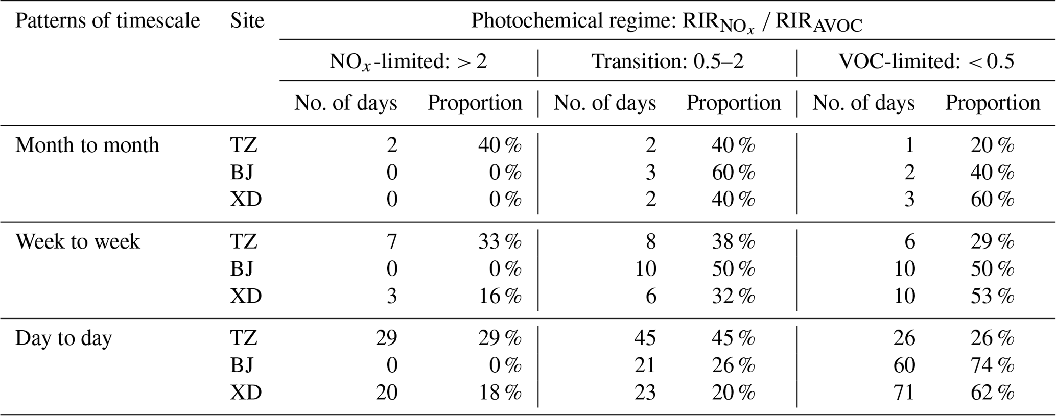
Table 2 summarizes the number of days and proportions that were classified into the three photochemical regimes across each site and each pattern of timescale. Near-consistent proportions of O3 formation regimes (using RIR RIRAVOC as a metric) were shown among multiple patterns of timescale, whereas a variability of proportion occurred among the three sites. The proportions of photochemical regimes changed according to the timescale that was varied from wider to narrower patterns. Taking TZ as an example, 20 % (monthly) and 26 % (daily) of the time was considered to be a VOC-limited regime. The number of days and proportions for the photochemical regimes summarized at four patterns of timescale can reveal a more plausible and comprehensive variation in ozone formation chemistry. Compared with patterns of monthly and weekly scales, the results derived at a daily scale can reveal the temporal variability of photochemical regimes more comprehensively. Note that the photochemical regime proportion obtained from the day-to-day scale has an advantage due to the large number of statistical samples.
Table 2Summary of the number of days (for model calculation) and proportions that were classified into the three photochemical regimes across each site and multiple patterns of timescale.
3.6 Comparison among different patterns of timescale
This section gives a more comprehensive understanding of the campaign-averaging O3–precursor relationship by comparing the similarities and differences of the results from various patterns of timescale. The overall O3–precursor relationship for the entire campaign can be quantified by averaging the RIR values from the individual simulation runs depending on the chosen timescale (e.g., five simulation runs for monthly scale in this study). Therefore, four sets of logical and comparable results can be derived to represent the campaign-averaging O3–precursor relationship, as four patterns of timescale (i.e., 5-month, monthly, weekly, and daily) were treated in this study.
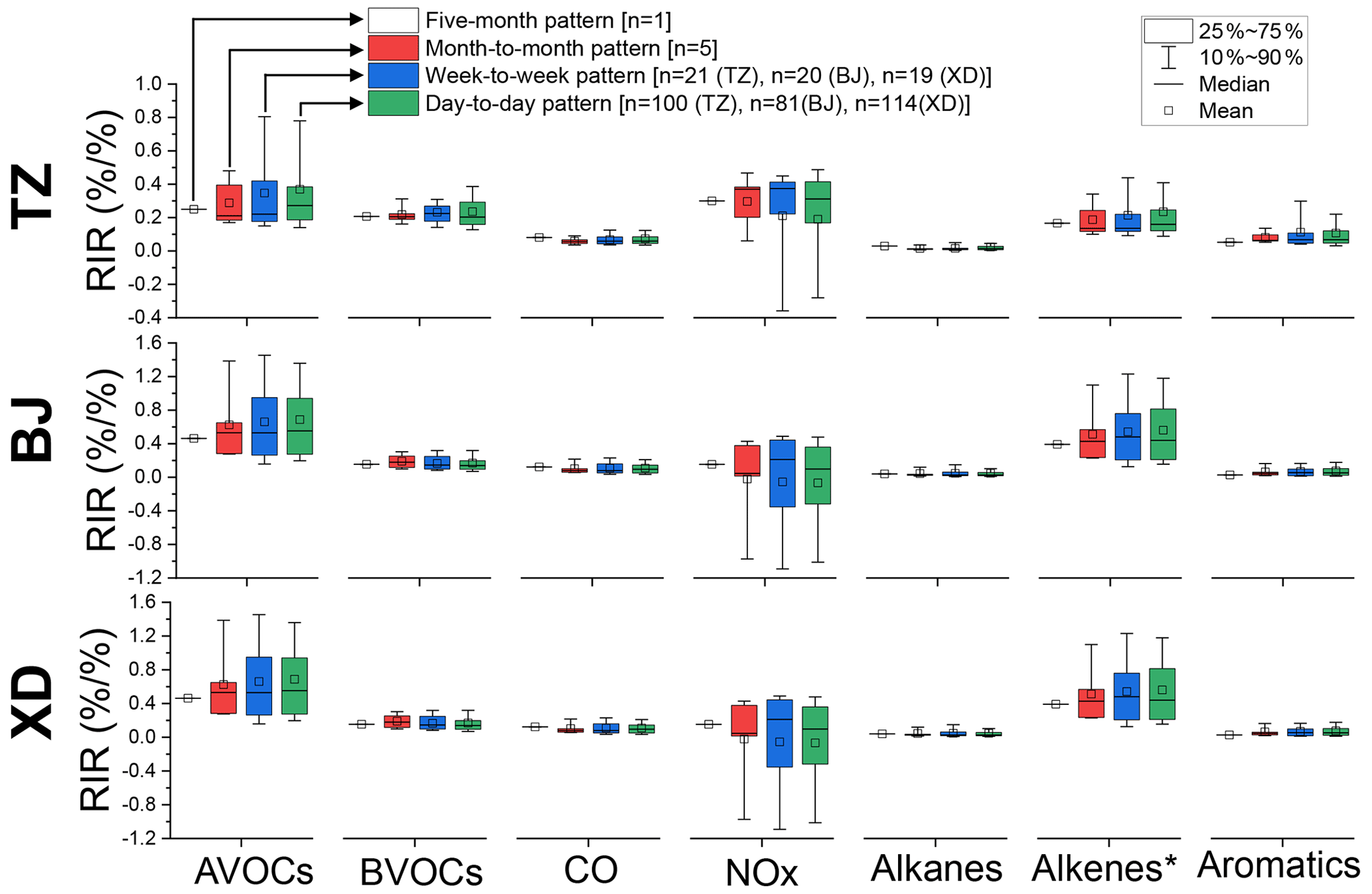
Figure 6Distribution of RIR values of major precursor groups in multiple patterns of timescale at three sites (TZ, BJ, and XD) in Zibo.
Figure 6 shows the averaged RIR values of the major precursor groups at different patterns of timescale. As the timescale changed from a wider (i.e., 5-month scale) to narrower (i.e., daily scale) pattern, all three sites showed increases in the means of RIRAVOC and RIR, as well as decreases in averaged RIR, whereas the averaged RIR of other precursors (i.e., BVOCs, CO, alkanes, and aromatics) did not vary obviously (see Table S6). Comparing with the O3–VOCs–NOx sensitivity at the daily scale, the results obtained at the 5-month scale underestimated O3–AVOCs sensitivity (indicated by averaged RIR values) by 48 % (TZ), 66 % (BJ), and 49 % (XD) and overestimated O3–NOx sensitivity by 37 % (TZ), 142 % (BJ), and 144 % (XD). We performed comprehensive uncertainty analysis for model input and output results, which was assessed through statistical methods (see details in Sect. 3.7). We found that the model-derived RIR values may become more uncertain when the input dataset was averaged into a wider diurnal pattern (i.e., 5-month scale), which may explain the discrepancy in RIR values between the 5-month scale and daily scale. We expect that such discrepancies derived from different patterns of timescale could widely exist in many other world areas. Note that the mean RIR values were generally consistent among the four patterns of timescale within a reasonable range (within the 25–75th quantile and standard deviation; see Fig. 6 and Table S4), suggesting that any selected pattern of timescale could reasonably derive the campaign-averaging O3–precursor relationship.
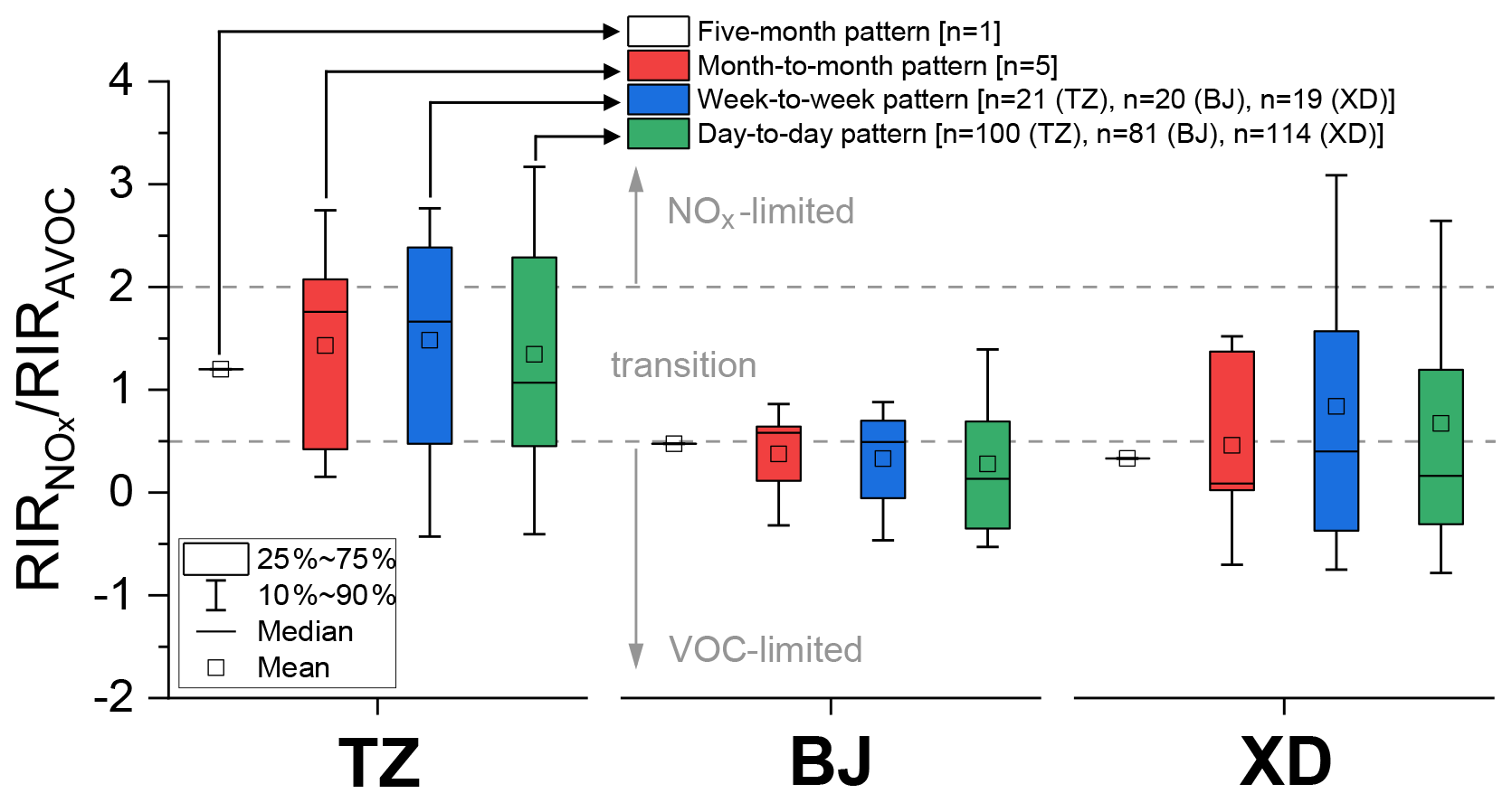
Figure 7Distribution of RIR RIRAVOC (indicator of photochemical regime) in multiple patterns of timescale at three sites (TZ, BJ, and XD) in Zibo.
Figure 7 further shows the variations in photochemical regimes (defined by RIR RIRAVOC; see Sect. S2 and Table S4 for details) for each pattern of timescale. Specifically, TZ was mainly considered to be a transitional regime for the entire campaign period, whereas its variations covered three photochemical regimes, which was consistent with the results from Table S6. BJ was generally identified as a VOC-limited regime, whereas some days were also grouped into a transitional regime. XD was considered to be primarily between a VOC-limited and transitional regime, and its variations also spanned three photochemical regimes. Compared with the 5-month pattern, it was further found that the averaged RIR RIRAVOC from other timescale patterns (i.e., monthly, weekly, and daily) was higher (12 % to 20 % for TZ; 38 % to 153 % for XD) or lower (21 % to 65 % for BJ) than that from the 5-month scale. Note that the above discrepancies in photochemical regime derived from multiple patterns of timescale may influence the development of targeted O3 control strategies. In summary, the photochemical regime derived by averaging RIR RIRAVOC from the daily scale (see Table S6) suggests that the three sites mainly followed the sequence of TZ (1.34±1.39) > XD (0.67±1.49) > BJ (0.16±0.65).
In addition, the temporal variations of TVOC NOx at different timescales were identified during the whole campaign, and good correlations between observed TVOC NOx and model-derived RIR RIRAVOC at four patterns of timescale were also found (see Fig. 5). Such consistency suggests that both metrics can reasonably reflect the variation of photochemical regimes, which can also improve the reliability of our box model simulation.
The consistency and difference of model output (summarized in Table S7) are quantified by the statistical methods of Pearson's correlation coefficient (Hu et al., 2018) and paired-samples t-test analysis (Wang et al., 2016). In particular, we assess and compare the degree of significance of the differences among multiple patterns of timescale by means of the p values (a statistical significance assuming that p < 0.05) through paired-samples t-tests and Wilcoxon matched-pairs signed-rank tests (non-parametric statistics; Chiclana et al., 2013). Figure 8a shows that high Pearson's correlation coefficients (with values all above 0.85, p < 0.01) were found among four patterns of timescale and that the higher correlation coefficient was identified between the two closer patterns. Figure 8b–c shows that the differences among multiple patterns of timescale were non-significant using paired-samples t-test analysis and Wilcoxon matched-pair signed-rank tests, respectively. Furthermore, their results indicate that a more significant difference was recognized between the two distant patterns (e.g., daily and 5-month), which is consistent with the results of Pearson's correlation analysis. It is noted that the discrepancy between the two distant patterns was not significant but non-negligible (e.g., p= 0.092 of the Wilcoxon matched-pairs signed-rank test between 5-month and daily patterns).
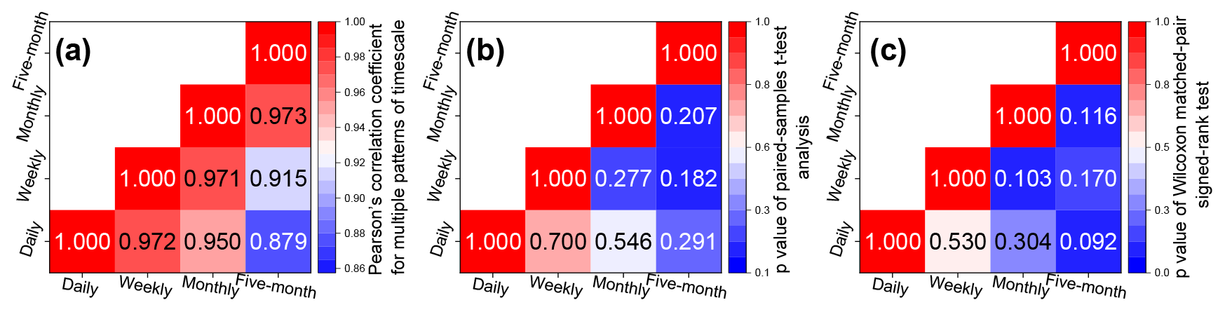
Figure 8The statistical analysis results of RIR values (from Table S6) at multiple patterns of timescale: (a) Pearson's r correlation analysis (all the results have passed statistical significance, assumed to be p < 0.01); (b) paired-samples t-test analysis (*p values refer to differences with a statistical significance assumed to be p < 0.05); (c) Wilcoxon matched-pairs signed-rank test (*p values refer to differences with a statistical significance, assumed to be p < 0.05).
The influence of different patterns of timescale on deriving RIR values from individual AVOC species was further investigated. Briefly, quantifying the relative contribution of individual AVOCs to O3 formation based on RIR calculation is beneficial to the development of cost-effective AVOC control strategies (Zhang et al., 2021). Figure 9 shows the averaged RIR values of individual AVOC species (i.e., top 10) at different patterns of timescale (i.e., 5-month, month to month, week to week) at three sites in Zibo. As shown in Fig. 9, the 10 individual AVOC species at the three sites were selected according to the top 10 highest RIR from the 5-month pattern. All three sites showed that the RIR of individual AVOC species increased gradually as the timescale changed from the wider (i.e., 5-month) to narrower (i.e., weekly) pattern, which was consistent with the earlier discussion (see Fig. 6 and Table S6) of O3–AVOC sensitivity derived from four patterns of timescale. The results also indicate that the choice of timescale pattern has a limited effect on deriving high-ranking AVOC species (i.e., top 10) based on RIR calculations.
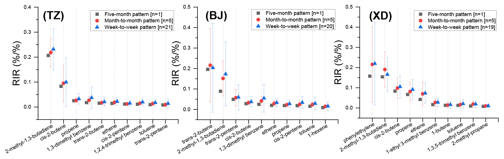
Figure 9Averaged RIR values of individual AVOC species (top 10) at different patterns of timescale at three sites (TZ, BJ, and XD) in Zibo. The error bars represent the standard deviations of the mean.
3.7 Uncertainty analysis
The uncertainty of model input, which is embedded in a pre-processed dataset with multiple patterns of timescale, was quantified in this section. As shown in Fig. 1, the daily simulation used the individual daily pattern to constrain the model, while the input dataset of averaged diurnal patterns (i.e., weekly, monthly, and 5-month) is treated by averaging the individual daily pattern into different timescales. This averaging approach will conceal the temporal variations of O3 precursors and meteorological factors, particularly for a long-term observational campaign. Figure S14 shows the distributions of the standard deviations for OH reactivity (kOH) or the concentration of O3 precursor groups at three averaged patterns of timescale at the three sites. As the timescale changed from a wider (i.e., 5-month scale) to narrower (i.e., weekly scale) pattern, the uncertainty (indicated by the average, median, and 25 %–75 % quantile) decreased accordingly. In addition, meteorological factors such as temperature and irradiation also play an important role in O3 formation, and it is specifically noted that these meteorological parameters can vary greatly over a long observational period (Boleti et al., 2020; Liu et al., 2019; Weng et al., 2022). Therefore, the masked temporal variation of these meteorological factors behind the averaged input dataset would also result in model uncertainty.
Moreover, it has been widely recognized that the uncertainty for 0-D box model simulation mainly arises from the constraint of observation datasets and the configuration of model schemes. Note that constraints with more species from measurements (or including as many species as possible) would lower its uncertainty from the chemical box model simulation (Wolfe et al., 2011, 2016). Nevertheless, due to the measurement limitation in our field campaign, we are unable to measure some important atmospheric species (i.e., HONO and oxygenated VOCs (OVOCs)), and these may raise uncertainty in the box model simulation. For instance, Xue et al. (2021) performed a sensitivity test for HONO constraint in their box model simulation, and they showed that no HONO constraint would lead to the O3 photochemical production rate decreasing by 42 %. More recently, Wang et al. (2022) obtained a comprehensive VOC dataset at Guangzhou, and their results showed that box model simulation without OVOC constraints would underestimate the productions of ROx and O3. Besides, both gaseous HNO3 and organic nitrates can result in interferences to NOx measurements by means of the chemiluminescence technique, which may raise uncertainty in our box modeling (Ge et al., 2022; Uno et al., 2017; Xu et al., 2013). Since the accurate NOx measurement is essential in determining the photochemical regime, more in-depth studies on NOx measurement uncertainty in box model simulations are required in the future. In addition, the parameter configuration of model schemes is essential to derive a reliable and valid model output, such as dilution rate as an important technical model parameter. We performed a stepwise sensitivity test for this parameter to obtain an optimized dilution rate and assigned it to all non-constraint species, which can reduce uncertainty in box model simulation (see details in Sect. S1). Also, the dry and/or wet deposition of pollutants is an important atmospheric physical process, which has been mostly parameterized in emission-based chemical transport modeling but is very limited in box modeling, as most of the primarily emitted species are already constrained from measurements. Xue et al. (2014c) considered O3 deposition in box model simulations, and their results showed a negligible contribution of O3 deposition to total O3 destruction rates. As for this work, we are unable to consider the deposition due to the difficulty in representing and parameterizing this term in the 0-D box model. Nevertheless, deposition of O3 and other species may be one of the uncertainties during box model simulation, which is worth further study in the future.
Our present results suggest that comprehensively understanding multiple patterns of timescale is conductive to formulating a more accurate and robust O3 control strategy. Specifically, as identified from the narrower patterns of timescale (i.e., weekly and daily), the site-to-site photochemical regime indicated by RIR RIRAVOC showed various magnitudes but a synchronous temporal trend. This indicates that the O3 formation regime in a city area can be influenced by local and regional emissions jointly. The reason behind this phenomenon is not clear at present, and we believe that further investigation on the synergetic effect of local and regional emission reduction for O3 control would help elucidate this observation. It was also found that the campaign-averaging photochemical regimes showed overall consistency but non-negligible variability among the four patterns of timescale, which was mainly due to the embedded uncertainty in the model input dataset with averaged diurnal patterns. This implies that comparison among multiple patterns of timescale based on RIR analysis is useful to derive the O3–precursor relationship more accurately and reliably.
Moreover, the high-ranking AVOC species (i.e., top 10) based on RIR calculations were overall consistent between the narrow to wide patterns of timescale. Table S8 summarizes the total run number of box models for different patterns of timescale. It is known that large-scale computing capacity and computational efficiency were required in the narrower pattern of timescale (e.g., 2760 simulation runs at the weekly scale in this study). Considering the difficulties of performing long-term and continuous online measurements in some environments, it is also advisable to identify the high-ranking VOC species from the campaign-averaging diurnal pattern in box model simulation.
In this study, we explored the non-linearity of the O3–precursor relationship in a way driven by the actual daily, weekly, and monthly variability around the distribution. Our results highlight the importance of quantitatively testing the impact of different timescales on photochemical regime determination, as there is uncertainty embedded in the model input dataset when averaging individual daily pattern into different timescales. Such understanding would be complementary in developing more accurate O3 pollution control strategies, particularly as the long-term O3–precursor observations (e.g., from several months to years) are becoming more available than before in many places throughout China. In addition, site-to-site differences of model-derived photochemical regimes also underline the importance of developing targeted O3 control strategies for different areas on a city scale. Specifically, according to the averaged RIR RIRAVOC of the daily pattern, the derived photochemical regime was transitional for TZ (suburban) and XD (suburban), while it was VOC-limited for BJ (urban). This implies that, for mitigating ozone pollution in the city of Zibo, more endeavors should be devoted to the anthropogenic VOC reduction in urban areas while strengthening the synergetic mitigation of VOC and NOx emissions at the same time in other suburban areas. Although the above implications for O3 control were derived from a case study in a major prefecture-level city (Zibo) of northern China, the approach of integrating multiple patterns of timescale developed in the present work can be used in other regions, particularly in relation to the ongoing “One City One Policy” campaign (2021–2023) for O3 control in many cities in China.
The code for the Master Chemical Mechanism (MCMv3.3.1) can be retrieved from http://mcm.york.ac.uk (MCM, 2023).
The datasets generated and analyzed during the current study are available on reasonable request from the corresponding author (Kangwei Li).
The supplement related to this article is available online at: https://doi.org/10.5194/acp-23-2649-2023-supplement.
KL conceived and led the study. ZZ performed the modeling. ZZ, KL, and ZB analyzed the data. BX, JD, LL, GZ, SL, CG, and WY conducted the field measurement. ZZ and KL wrote the paper. MA and ZB commented on the paper.
The contact author has declared that none of the authors has any competing interests.
Publisher's note: Copernicus Publications remains neutral with regard to jurisdictional claims in published maps and institutional affiliations.
We thank William Bloss for the initial check and helpful comments.
This work was supported by National Center for Air Pollution Prevention and Control (grant no. DQGG202119) and Ministry of Science and Technology PRC (grant nos. G20200160001 and G2021060002L).
This paper was edited by Tao Wang and reviewed by two anonymous referees.
Blanchard, C. L.: Ozone process insights from field experiments – Part III: extent of reaction and ozone formation, Atmos. Environ., 34, 2035–2043, https://doi.org/10.1016/S1352-2310(99)00458-6, 2000.
Boleti, E., Hueglin, C., Grange, S. K., Prévôt, A. S. H., and Takahama, S.: Temporal and spatial analysis of ozone concentrations in Europe based on timescale decomposition and a multi-clustering approach, Atmos. Chem. Phys., 20, 9051–9066, https://doi.org/10.5194/acp-20-9051-2020, 2020.
Brunekreef, B. and Holgate, S. T.: Air pollution and health, Lancet, 360, 1233–1242, https://doi.org/10.1016/S0140-6736(02)11274-8, 2002.
Cardelino, C. A. and Chameides, W. L.: An observation-based model for analyzing ozone precursor relationships in the urban atmosphere, J. Air Waste Ma., 45, 161–180, https://doi.org/10.1080/10473289.1995.10467356, 1995.
Carter, W. P. L.: Development of the SAPRC-07 chemical mechanism, Atmos. Environ., 44, 5324–5335, https://doi.org/10.1016/j.atmosenv.2010.01.026, 2010.
Cheng, H., Guo, H., Wang, X., Saunders, S. M., Lam, S. H. M., Jiang, F., Wang, T., Ding, A., Lee, S., and Ho, K. F.: On the relationship between ozone and its precursors in the Pearl River Delta: Application of an observation-based model (OBM), Environ. Sci. Pollut. R., 17, 547–560, https://doi.org/10.1007/s11356-009-0247-9, 2010.
Chiclana, F., García, J. M. T., del Moral, M. J., and Herrera-Viedma, E.: A statistical comparative study of different similarity measures of consensus in group decision making, Inf. Sci. (Ny), 221, 110–123, 2013.
Chien, Y.-C.: Variations in amounts and potential sources of volatile organic chemicals in new cars, Sci. Total Environ., 382, 228–239, https://doi.org/10.1016/j.scitotenv.2007.04.022, 2007.
Fan, M. Y., Zhang, Y. L., Lin, Y. C., Li, L., Xie, F., Hu, J., Mozaffar, A., and Cao, F.: Source apportionments of atmospheric volatile organic compounds in Nanjing, China during high ozone pollution season, Chemosphere, 263, 128025, https://doi.org/10.1016/j.chemosphere.2020.128025, 2021.
Ge, D., Nie, W., Sun, P., Liu, Y., Wang, T., Wang, J., Wang, J., Wang, L., Zhu, C., and Wang, R.: Characterization of particulate organic nitrates in the Yangtze River Delta, East China, using the time-of-flight aerosol chemical speciation monitor, Atmos. Environ., 272, 118927, https://doi.org/10.1016/j.atmosenv.2021.118927, 2022.
Goliff, W. S., Stockwell, W. R., and Lawson, C. V: The regional atmospheric chemistry mechanism, version 2, Atmos. Environ., 68, 174–185, https://doi.org/10.1016/j.atmosenv.2012.11.038, 2013.
He, Z., Wang, X., Ling, Z., Zhao, J., Guo, H., Shao, M., and Wang, Z.: Contributions of different anthropogenic volatile organic compound sources to ozone formation at a receptor site in the Pearl River Delta region and its policy implications, Atmos. Chem. Phys., 19, 8801–8816, https://doi.org/10.5194/acp-19-8801-2019, 2019.
Hidy, G. M.: Ozone process insights from field experiments – part I: Overview, Atmos. Environ., 34, 2001–2022, https://doi.org/10.1016/S1352-2310(99)00456-2, 2000.
Hu, H., Landgraf, J., Detmers, R., Borsdorff, T., Aan de Brugh, J., Aben, I., Butz, A., and Hasekamp, O.: Toward global mapping of methane with TROPOMI: First results and intersatellite comparison to GOSAT, Geophys. Res. Lett., 45, 3682–3689, 2018.
Jenkin, M. E., Young, J. C., and Rickard, A. R.: The MCM v3.3.1 degradation scheme for isoprene, Atmos. Chem. Phys., 15, 11433–11459, https://doi.org/10.5194/acp-15-11433-2015, 2015.
Jiang, M., Lu, K., Su, R., Tan, Z., Wang, H., Li, L., Fu, Q., Zhai, C., Tan, Q., and Yue, D.: Ozone formation and key VOCs in typical Chinese city clusters, Chinese Sci. Bull., 63, 1130–1141, 2018.
Kleinman, L. I.: Ozone process insights from field experiments – part II: Observation-based analysis for ozone production, Atmos. Environ., 34, 2023–2033, https://doi.org/10.1016/S1352-2310(99)00457-4, 2000.
Li, J., Zhai, C., Yu, J., Liu, R., Li, Y., Zeng, L., and Xie, S.: Spatiotemporal variations of ambient volatile organic compounds and their sources in Chongqing, a mountainous megacity in China, Sci. Total Environ., 627, 1442–1452, 2018.
Li, K., Jacob, D. J., Liao, H., Shen, L., Zhang, Q., and Bates, K. H.: Anthropogenic drivers of 2013–2017 trends in summer surface ozone in China, P. Natl. Acad. Sci. USA, 116, 422–427, https://doi.org/10.1073/pnas.1812168116, 2019.
Li, K., Wang, X., Li, L., Wang, J., Liu, Y., Cheng, X., Xu, B., Wang, X., Yan, P., Li, S., Geng, C., Yang, W., Azzi, M., and Bai, Z.: Large variability of O3-precursor relationship during severe ozone polluted period in an industry-driven cluster city (Zibo) of North China Plain, J. Clean. Prod., 316, 128252, https://doi.org/10.1016/j.jclepro.2021.128252, 2021.
Lin, H., Wang, M., Duan, Y., Fu, Q., Ji, W., Cui, H., Jin, D., Lin, Y., and Hu, K.: O3 sensitivity and contributions of different nmhc sources in O3 formation at urban and suburban sites in Shanghai, Atmosphere, 11, 295, https://doi.org/10.3390/atmos11030295, 2020.
Ling, Z. H., Guo, H., Cheng, H. R., and Yu, Y. F.: Sources of ambient volatile organic compounds and their contributions to photochemical ozone formation at a site in the Pearl River Delta, southern China, Environ. Pollut., 159, 2310–2319, https://doi.org/10.1016/j.envpol.2011.05.001, 2011.
Liu, X., Lyu, X., Wang, Y., Jiang, F., and Guo, H.: Intercomparison of O3 formation and radical chemistry in the past decade at a suburban site in Hong Kong, Atmos. Chem. Phys., 19, 5127–5145, https://doi.org/10.5194/acp-19-5127-2019, 2019.
Liu, X., Wang, N., Lyu, X., Zeren, Y., Jiang, F., Wang, X., Zou, S., Ling, Z., and Guo, H.: Photochemistry of ozone pollution in autumn in Pearl River Estuary, South China, Sci. Total Environ., 754, 141812, https://doi.org/10.1016/j.scitotenv.2020.141812, 2021a.
Liu, X., Wang, N., Lyu, X., Zeren, Y., Jiang, F., Wang, X., Zou, S., Ling, Z., and Guo, H.: Photochemistry of ozone pollution in autumn in Pearl River Estuary, South China, Sci. Total Environ., 754, 141812, https://doi.org/10.1016/j.scitotenv.2020.141812, 2021b.
Lu, H., Lyu, X., Cheng, H., Ling, Z., Guo, H., and Lu, H.: Overview on the spatial–temporal characteristics of the ozone formation regime in China, Environ. Sci., 21, 916–929, https://doi.org/10.1039/c9em00098d, 2019.
Lu, K., Zhang, Y., Su, H., Brauers, T., Chou, C. C., Hofzumahaus, A., Liu, S. C., Kita, K., Kondo, Y., Shao, M., Wahner, A., Wang, J., Wang, X., and Zhu, T.: Oxidant (O3 + NO2) production processes and formation regimes in Beijing, J. Geophys. Res.-Atmos., 115, D07303, https://doi.org/10.1029/2009JD012714, 2010a.
Lu, K., Zhang, Y., Su, H., Shao, M., Zeng, L., Zhong, L., Xiang, Y., Chang, C., Chou, C. K. C., and Wahner, A.: Regional ozone pollution and key controlling factors of photochemical ozone production in Pearl River Delta during summer time, Sci. China Chem., 53, 651–663, https://doi.org/10.1007/s11426-010-0055-6, 2010b.
Lu, X., Hong, J., Zhang, L., Cooper, O. R., Schultz, M. G., Xu, X., Wang, T., Gao, M., Zhao, Y., and Zhang, Y.: Severe Surface Ozone Pollution in China: A Global Perspective, Environ. Sci. Tech. Let., 5, 487–494, https://doi.org/10.1021/acs.estlett.8b00366, 2018.
Lyu, X., Wang, N., Guo, H., Xue, L., Jiang, F., Zeren, Y., Cheng, H., Cai, Z., Han, L., and Zhou, Y.: Causes of a continuous summertime O3 pollution event in Jinan, a central city in the North China Plain, Atmos. Chem. Phys., 19, 3025–3042, https://doi.org/10.5194/acp-19-3025-2019, 2019.
Lyu, X. P., Chen, N., Guo, H., Zhang, W. H., Wang, N., Wang, Y., and Liu, M.: Ambient volatile organic compounds and their effect on ozone production in Wuhan, central China, Sci. Total Environ., 541, 200–209, https://doi.org/10.1016/j.scitotenv.2015.09.093, 2016.
MCM – The Master Chemical Mechanism: Welcome to the MCM website, http://mcm.york.ac.uk, last access: 27 January 2023.
National Research Council: Rethinking the Ozone Problem in Urban and Regional Air Pollution, The National Academies Press, Washington, DC, ISBN 978-0309046312, 1991.
Qin, M., Chen, Z., Shen, H., Li, H., Wu, H., and Wang, Y.: Impacts of heterogeneous reactions to atmospheric peroxides: Observations and budget analysis study, Atmos. Environ., 183, 144–153, https://doi.org/10.1016/j.atmosenv.2018.04.005, 2018.
Saunders, S. M., Jenkin, M. E., Derwent, R. G., and Pilling, M. J.: Protocol for the development of the Master Chemical Mechanism, MCM v3 (Part A): tropospheric degradation of non-aromatic volatile organic compounds, Atmos. Chem. Phys., 3, 161–180, https://doi.org/10.5194/acp-3-161-2003, 2003.
Sicard, P., De Marco, A., Agathokleous, E., Feng, Z., Xu, X., Paoletti, E., Rodriguez, J. J. D., and Calatayud, V.: Amplified ozone pollution in cities during the COVID-19 lockdown, Sci. Total Environ., 735, 139542, https://doi.org/10.1016/j.scitotenv.2020.139542, 2020.
Sillman, S.: Observation-Based Methods (OBMS) For Analyzing Urban/Regional Ozone Production And Ozone-NOx-VOC Sensitivity, http://www-personal.umich.edu/~sillman/obm.htm (last access: 17 February 2023), 2010.
Stockwell, W. R., Kirchner, F., Kuhn, M., and Seefeld, S.: A new mechanism for regional atmospheric chemistry modeling, J. Geophys. Res.-Atmos., 102, 25847–25879, https://doi.org/10.1029/97jd00849, 1997.
Stockwell, W. R., Saunders, E., Goliff, W. S., and Fitzgerald, R. M.: A perspective on the development of gas-phase chemical mechanisms for Eulerian air quality models, J. Air Waste Ma., 70, 44–70, 2020.
Su, R., Lu, K., Yu, J., Tan, Z., Jiang, M., Li, J., Xie, S., Wu, Y., Zeng, L., and Zhai, C.: Exploration of the formation mechanism and source attribution of ambient ozone in Chongqing with an observation-based model, Sci. China Earth Sci., 61, 23–32, 2018a.
Su, R., Lu, K. D., Yu, J. Y., Tan, Z. F., Jiang, M. Q., Li, J., Xie, S. D., Wu, Y. S., Zeng, L. M., Zhai, C. Z., and Zhang, Y. H.: Exploration of the formation mechanism and source attribution of ambient ozone in Chongqing with an observation-based model, Sci. China Earth Sci., 61, 23–32, https://doi.org/10.1007/s11430-017-9104-9, 2018b.
Sun, L., Xue, L., Wang, T., Gao, J., Ding, A., Cooper, O. R., Lin, M., Xu, P., Wang, Z., Wang, X., Wen, L., Zhu, Y., Chen, T., Yang, L., Wang, Y., Chen, J., and Wang, W.: Significant increase of summertime ozone at Mount Tai in Central Eastern China, Atmos. Chem. Phys., 16, 10637–10650, https://doi.org/10.5194/acp-16-10637-2016, 2016.
Tan, Z., Lu, K., Dong, H., Hu, M., Li, X., Liu, Y., Lu, S., Shao, M., Su, R., and Wang, H.: Explicit diagnosis of the local ozone production rate and the ozone-NOx-VOC sensitivities, Sci. Bull., 63, 1067–1076, 2018a.
Tan, Z., Lu, K., Jiang, M., Su, R., Dong, H., Zeng, L., Xie, S., Tan, Q., and Zhang, Y.: Exploring ozone pollution in Chengdu, southwestern China: A case study from radical chemistry to O3-VOC-NOx sensitivity, Sci. Total Environ., 636, 775–786, 2018b.
Tan, Z., Lu, K., Jiang, M., Su, R., Wang, H., Lou, S., Fu, Q., Zhai, C., Tan, Q., Yue, D., Chen, D., Wang, Z., Xie, S., Zeng, L., and Zhang, Y.: Daytime atmospheric oxidation capacity in four Chinese megacities during the photochemically polluted season: a case study based on box model simulation, Atmos. Chem. Phys., 19, 3493–3513, https://doi.org/10.5194/acp-19-3493-2019, 2019.
Uno, I., Osada, K., Yumimoto, K., Wang, Z., Itahashi, S., Pan, X., Hara, Y., Kanaya, Y., Yamamoto, S., and Fairlie, T. D.: Seasonal variation of fine- and coarse-mode nitrates and related aerosols over East Asia: synergetic observations and chemical transport model analysis, Atmos. Chem. Phys., 17, 14181–14197, https://doi.org/10.5194/acp-17-14181-2017, 2017.
Vingarzan, R.: A review of surface ozone background levels and trends, Atmos. Environ., 38, 3431–3442, 2004.
Wang, H., Hu, X. and Sterba-Boatwright, B.: A new statistical approach for interpreting oceanic fCO2 data, Mar. Chem., 183, 41–49, 2016.
Wang, M., Hu, K., Chen, W., Shen, X., Li, W., and Lu, X.: Ambient Non-Methane Hydrocarbons (NMHCs) Measurements in Baoding, China: Sources and Roles in Ozone Formation, Atmosphere, 11, 1205, https://doi.org/10.3390/atmos11111205, 2020.
Wang, P., Chen, Y., Hu, J., Zhang, H., and Ying, Q.: Attribution of Tropospheric Ozone to NOx and VOC Emissions: Considering Ozone Formation in the Transition Regime, Environ. Sci. Technol., 53, 1404–1412, https://doi.org/10.1021/acs.est.8b05981, 2019.
Wang, T., Xue, L., Brimblecombe, P., Lam, Y. F., Li, L., and Zhang, L.: Ozone pollution in China: A review of concentrations, meteorological influences, chemical precursors, and effects, Sci. Total Environ., 575, 1582–1596, https://doi.org/10.1016/j.scitotenv.2016.10.081, 2017.
Wang, W., Yuan, B., Peng, Y., Su, H., Cheng, Y., Yang, S., Wu, C., Qi, J., Bao, F., Huangfu, Y., Wang, C., Ye, C., Wang, Z., Wang, B., Wang, X., Song, W., Hu, W., Cheng, P., Zhu, M., Zheng, J., and Shao, M.: Direct observations indicate photodegradable oxygenated volatile organic compounds (OVOCs) as larger contributors to radicals and ozone production in the atmosphere, Atmos. Chem. Phys., 22, 4117–4128, https://doi.org/10.5194/acp-22-4117-2022, 2022.
Wang, Y., Wang, H., Guo, H., Lyu, X., Cheng, H., Ling, Z., Louie, P. K. K., Simpson, I. J., Meinardi, S., and Blake, D. R.: Long-term O3–precursor relationships in Hong Kong: field observation and model simulation, Atmos. Chem. Phys., 17, 10919–10935, https://doi.org/10.5194/acp-17-10919-2017, 2017.
Wang, Y., Guo, H., Zou, S., Lyu, X., Ling, Z., Cheng, H., and Zeren, Y.: Surface O3 photochemistry over the South China Sea: Application of a near-explicit chemical mechanism box model, Environ. Pollut., 234, 155–166, https://doi.org/10.1016/j.envpol.2017.11.001, 2018.
Wang, Y., Gao, W., Wang, S., Song, T., Gong, Z., Ji, D., Wang, L., Liu, Z., Tang, G., Huo, Y., Tian, S., Li, J., Li, M., Yang, Y., Chu, B., Petäjä, T., Kerminen, V. M., He, H., Hao, J., Kulmala, M., Wang, Y., and Zhang, Y.: Contrasting trends of PM2.5 and surface-ozone concentrations in China from 2013 to 2017, Nat. Sci. Rev., 7, 1331–1339, https://doi.org/10.1093/nsr/nwaa032, 2020.
Weng, X., Forster, G. L., and Nowack, P.: A machine learning approach to quantify meteorological drivers of ozone pollution in China from 2015 to 2019, Atmos. Chem. Phys., 22, 8385–8402, https://doi.org/10.5194/acp-22-8385-2022, 2022.
Whalley, L. K., Slater, E. J., Woodward-Massey, R., Ye, C., Lee, J. D., Squires, F., Hopkins, J. R., Dunmore, R. E., Shaw, M., Hamilton, J. F., Lewis, A. C., Mehra, A., Worrall, S. D., Bacak, A., Bannan, T. J., Coe, H., Percival, C. J., Ouyang, B., Jones, R. L., Crilley, L. R., Kramer, L. J., Bloss, W. J., Vu, T., Kotthaus, S., Grimmond, S., Sun, Y., Xu, W., Yue, S., Ren, L., Acton, W. J. F., Hewitt, C. N., Wang, X., Fu, P., and Heard, D. E.: Evaluating the sensitivity of radical chemistry and ozone formation to ambient VOCs and NOx in Beijing, Atmos. Chem. Phys., 21, 2125–2147, https://doi.org/10.5194/acp-21-2125-2021, 2021.
Willmott, C. J.: Some comments on the evaluation of model performance, B. Am. Meteorol. Soc., 63, 1309–1313, https://doi.org/10.1175/1520-0477(1982)063<1309:SCOTEO>2.0.CO;2, 1982.
Wolfe, G. M., Thornton, J. A., Bouvier-Brown, N. C., Goldstein, A. H., Park, J.-H., McKay, M., Matross, D. M., Mao, J., Brune, W. H., LaFranchi, B. W., Browne, E. C., Min, K.-E., Wooldridge, P. J., Cohen, R. C., Crounse, J. D., Faloona, I. C., Gilman, J. B., Kuster, W. C., de Gouw, J. A., Huisman, A., and Keutsch, F. N.: The Chemistry of Atmosphere-Forest Exchange (CAFE) Model – Part 2: Application to BEARPEX-2007 observations, Atmos. Chem. Phys., 11, 1269–1294, https://doi.org/10.5194/acp-11-1269-2011, 2011.
Wolfe, G. M., Marvin, M. R., Roberts, S. J., Travis, K. R., and Liao, J.: The Framework for 0-D Atmospheric Modeling (F0AM) v3.1, Geosci. Model Dev., 9, 3309–3319, https://doi.org/10.5194/gmd-9-3309-2016, 2016.
Xie, X., Shao, M., Liu, Y., Lu, S., Chang, C.-C., and Chen, Z.-M.: Estimate of initial isoprene contribution to ozone formation potential in Beijing, China, Atmos. Environ., 42, 6000–6010, 2008.
Xu, Z., Wang, T., Xue, L. K., Louie, P. K. K., Luk, C. W. Y., Gao, J., Wang, S. L., Chai, F. H., and Wang, W. X.: Evaluating the uncertainties of thermal catalytic conversion in measuring atmospheric nitrogen dioxide at four differently polluted sites in China, Atmos. Environ., 76, 221–226, 2013.
Xu, Z., Huang, X., Nie, W., Chi, X., Xu, Z., Zheng, L., Sun, P., and Ding, A.: Influence of synoptic condition and holiday effects on VOCs and ozone production in the Yangtze River Delta region, China, Atmos. Environ., 168, 112–124, 2017.
Xue, L., Wang, T., Louie, P. K. K., Luk, C. W. Y., Blake, D. R., and Xu, Z.: Increasing external effects negate local efforts to control ozone air pollution: a case study of Hong Kong and implications for other Chinese cities, Environ. Sci. Technol., 48, 10769–10775, 2014a.
Xue, L., Wang, T., Louie, P. K. K., Luk, C. W. Y., Blake, D. R., and Xu, Z.: Increasing external effects negate local efforts to control ozone air pollution: A case study of Hong Kong and implications for other chinese cities, Environ. Sci. Technol., 48, 10769–10775, https://doi.org/10.1021/es503278g, 2014b.
Xue, L. K., Wang, T., Gao, J., Ding, A. J., Zhou, X. H., Blake, D. R., Wang, X. F., Saunders, S. M., Fan, S. J., Zuo, H. C., Zhang, Q. Z., and Wang, W. X.: Ground-level ozone in four Chinese cities: precursors, regional transport and heterogeneous processes, Atmos. Chem. Phys., 14, 13175–13188, https://doi.org/10.5194/acp-14-13175-2014, 2014c.
Xue, M., Ma, J., Tang, G., Tong, S., Hu, B., Zhang, X., Li, X., and Wang, Y.: ROx Budgets and O3 Formation during Summertime at Xianghe Suburban Site in the North China Plain, Adv. Atmos. Sci., 38, 1209–1222, 2021.
Xue, T., Zheng, Y., Geng, G., Xiao, Q., Meng, X., Wang, M., Li, X., Wu, N., Zhang, Q., and Zhu, T.: Estimating Spatiotemporal Variation in Ambient Ozone Exposure during 2013–2017 Using a Data-Fusion Model, Environ. Sci. Technol., 54, 14877–14888, 2020.
Yarwood, G., Rao, S., Yocke, M., and Whitten, G. Z.: Updates to the carbon bond chemical mechanism: CB05, Final Rep. to US EPA, RT-0400675, 8, 13, ISBN RT-04-00675, 2005.
Yarwood, G., Jung, J., Whitten, G. Z., Heo, G., Mellberg, J., and Estes, M.: Updates to the Carbon Bond mechanism for version 6 (CB6), in: 9th Annual CMAS Conference, Chapel Hill, NC, 11–13, https://www.cmascenter.org/conference/2010/abstracts/emery_updates_carbon_2010.pdf (last access: 17 February 2023), 2010.
Yin, M., Zhang, X., Li, Y., Fan, K., Li, H., Gao, R., and Li, J.: Ambient ozone pollution at a coal chemical industry city in the border of Loess Plateau and Mu Us Desert: characteristics, sensitivity analysis and control strategies, PeerJ, 9, e11322, https://doi.org/10.7717/peerj.11322, 2021.
Yu, D., Tan, Z., Lu, K., Ma, X., Li, X., Chen, S., Zhu, B., Lin, L., Li, Y., Qiu, P., Yang, X., Liu, Y., Wang, H., He, L., Huang, X., and Zhang, Y.: An explicit study of local ozone budget and NOx-VOCs sensitivity in Shenzhen China, Atmos. Environ., 224, 117304, https://doi.org/10.1016/j.atmosenv.2020.117304, 2020a.
Yu, D., Tan, Z., Lu, K., Ma, X., Li, X., Chen, S., Zhu, B., Lin, L., Li, Y., Qiu, P., Yang, X., Liu, Y., Wang, H., He, L., Huang, X., and Zhang, Y.: An explicit study of local ozone budget and NOx-VOCs sensitivity in Shenzhen China, Atmos. Environ., 224, 117304, https://doi.org/10.1016/j.atmosenv.2020.117304, 2020b.
Zeng, L., Lyu, X., Guo, H., Zou, S., and Ling, Z.: Photochemical Formation of C1-C5 Alkyl Nitrates in Suburban Hong Kong and over the South China Sea, Environ. Sci. Technol., 52, 5581–5589, https://doi.org/10.1021/acs.est.8b00256, 2018.
Zhang, Q., Zheng, Y., Tong, D., Shao, M., Wang, S., Zhang, Y., Xu, X., Wang, J., He, H., Liu, W., Ding, Y., Lei, Y., Li, J., Wang, Z., Zhang, X., Wang, Y., Cheng, J., Liu, Y., Shi, Q., Yan, L., Geng, G., Hong, C., Li, M., Liu, F., Zheng, B., Cao, J., Ding, A., Gao, J., Fu, Q., Huo, J., Liu, B., Liu, Z., Yang, F., He, K., and Hao, J.: Drivers of improved PM2.5 air quality in China from 2013 to 2017, P. Natl. Acad. Sci. USA, 116, 24463–24469, https://doi.org/10.1073/pnas.1907956116, 2019.
Zhang, Y., Xue, L., Carter, W. P. L., Pei, C., Chen, T., Mu, J., Wang, Y., Zhang, Q., and Wang, W.: Development of ozone reactivity scales for volatile organic compounds in a Chinese megacity, Atmos. Chem. Phys., 21, 11053–11068, https://doi.org/10.5194/acp-21-11053-2021, 2021.
Zhang, Y. H., Hu, M., Zhong, L. J., Wiedensohler, A., Liu, S. C., Andreae, M. O., Wang, W., and Fan, S. J.: Regional Integrated Experiments on Air Quality over Pearl River Delta 2004 (PRIDE-PRD2004): Overview, Atmos. Environ., 42, 6157–6173, https://doi.org/10.1016/j.atmosenv.2008.03.025, 2008a.
Zhang, Y. H., Su, H., Zhong, L. J., Cheng, Y. F., Zeng, L. M., Wang, X. S., Xiang, Y. R., Wang, J. L., Gao, D. F., Shao, M., Fan, S. J., and Liu, S. C.: Regional ozone pollution and observation-based approach for analyzing ozone–precursor relationship during the PRIDE-PRD2004 campaign, Atmos. Environ., 42, 6203–6218, https://doi.org/10.1016/j.atmosenv.2008.05.002, 2008b.
Zhao, Y., Chen, L., Li, K., Han, L., Zhang, X., Wu, X., Gao, X., Azzi, M., and Cen, K.: Atmospheric ozone chemistry and control strategies in Hangzhou, China: Application of a 0-D box model, Atmos. Res., 246, 105109, https://doi.org/10.1016/j.atmosres.2020.105109, 2020.
Zong, R., Yang, X., Wen, L., Xu, C., Zhu, Y., Chen, T., Yao, L., Wang, L., Zhang, J., Yang, L., Wang, X., Shao, M., Zhu, T., Xue, L., and Wang, W.: Strong ozone production at a rural site in theNorth China Plain: Mixed effects of urban plumesand biogenic emissions, J. Environ. Sci. (China), 71, 261–270, https://doi.org/10.1016/j.jes.2018.05.003, 2018.