the Creative Commons Attribution 4.0 License.
the Creative Commons Attribution 4.0 License.
 | 14 Dec 2023
The sensitivity of Southern Ocean atmospheric dimethyl sulfide (DMS) to modeled oceanic DMS concentrations and emissions
Yusuf A. Bhatti
Laura E. Revell
Alex J. Schuddeboom
Adrian J. McDonald
Alex T. Archibald
Jonny Williams
Abhijith U. Venugopal
Catherine Hardacre
Erik Behrens
The biogeochemical formation of dimethyl sulfide (DMS) from the Southern Ocean is complex, dynamic, and driven by physical, chemical, and biological processes. Such processes, produced by marine biogenic activity, are the dominant source of sulfate aerosol over the Southern Ocean. Using an atmosphere-only configuration of the United Kingdom Earth System Model (UKESM1-AMIP), we performed eight 10-year simulations for the recent past (2009–2018) during austral summer. We tested the sensitivity of atmospheric DMS to four oceanic DMS datasets and three DMS transfer velocity parameterizations. One oceanic DMS dataset was developed here from satellite chlorophyll a. We find that the choice of oceanic DMS dataset has a larger influence on atmospheric DMS than the choice of DMS transfer velocity. Simulations with linear transfer velocity parameterizations show a more accurate representation of atmospheric DMS concentration than those using quadratic relationships. This work highlights that the oceanic DMS and DMS transfer velocity parameterizations currently used in climate models are poorly constrained for the Southern Ocean region. Simulations using oceanic DMS derived from satellite chlorophyll a data, and when combined with a recently developed linear transfer velocity parameterization for DMS, show better spatial variability than the UKESM1 configuration. We also demonstrate that capturing large-scale spatial variability can be more important than large-scale interannual variability. We recommend that models use a DMS transfer velocity parameterization that was developed specifically for DMS and improvements to oceanic DMS spatial variability. Such improvements may provide a more accurate process-based representation of oceanic and atmospheric DMS, and therefore sulfate aerosol, in the Southern Ocean region.
- Article
(6490 KB) - Full-text XML
-
Supplement
(2216 KB) - BibTeX
- EndNote


The representation of aerosols over the Southern Ocean (40 to 60 ∘ S) is a large source of uncertainty in climate models due to the lack of observational data and large seasonal variability (Revell et al., 2019). Poor representation of aerosols contributes to the large biases in future climate projections over the Southern Ocean (Myhre et al., 2014). Sea spray and dimethyl sulfide (DMS; CH3SCH3) are fundamental sources for aerosol formation over this region (Revell et al., 2021; Bhatti et al., 2022). The dominant source of sulfate over the marine atmosphere is the biogenic marine aerosol precursor DMS (Keller et al., 1989; Bates et al., 1987; Kiene and Bates, 1990; Curson et al., 2011). Revell et al. (2019) found that sulfate aerosol production from DMS was responsible for around 60 % of the austral summer aerosol optical depth over the Southern Ocean. Atmospheric DMS therefore has the potential to greatly influence cloud condensation nuclei during austral summer (Kloster et al., 2006; Revell et al., 2019; Korhonen et al., 2008; Pandis et al., 1994).
The Southern Ocean contains extremely high phytoplankton and marine biota productivity during austral summer (DJF or December–February) (Deppeler and Davidson, 2017). Marine biogenic activity, controlled by marine biota, plays a key role in chlorophyll a (chl a) production and is considered to be a key driver of oceanic DMS production (e.g., Uhlig et al., 2019; Townsend and Keller, 1996; Anderson et al., 2001; Deppeler and Davidson, 2017). Earth system models (ESMs) represent the process of oceanic DMS formation through multiple approaches that are dependent on chl a, nutrients, light, mixed-layer depth, zooplankton, and dimethylsulfoniopropionate concentration (Bock et al., 2021). The UKESM1 and MIROC-ES2L models use a diagnostic approach to represent chl a (Sellar et al., 2019; Anderson et al., 2001; Hajima et al., 2020). The CNRM-ESM2-1 and NorESM2-LM models use a prognostic approach, closely related to zooplankton and dimethylsulfoniopropionate abundance, which is a precursor of oceanic DMS (Seland et al., 2020; Séférian et al., 2019). Bock et al. (2021) evaluated oceanic DMS in the Coupled Model Intercomparison Project Phase 6 (CMIP6) and found that all models are biased in comparison with observational climatologies of DMS in the Southern Ocean region.
Atmosphere-only global climate models use climatologies to prescribe the global concentration of oceanic DMS in the surface seawater layer. Lana et al. (2011), Kettle et al. (1999), and Hulswar et al. (2022) constructed observational climatologies of oceanic DMS, which are used by such models. However, there is a limited amount of data available within the Southern Ocean, which can lead to errors in the representation of oceanic DMS (e.g., Bock et al., 2021; Mulcahy et al., 2020). A limitation of representing oceanic DMS as a static climatology is that it does not account for the large temporal variations in DMS concentrations observed. For instance, El Niño–Southern Oscillation (ENSO) events, wildfires, and volcanic eruptions all significantly influence oceanic DMS within the Southern Ocean (e.g., Yoder and Kennelly, 2003; Tang et al., 2021; Wang et al., 2022; Browning et al., 2015; Longman et al., 2022). Calculating oceanic DMS online using a biological proxy would resolve these perturbing events to some degree (Galí et al., 2018).
The flux of DMS from the ocean to the atmosphere depends on the gas transfer velocity (K), which in turn depends on the surface wind speed (e.g., Fairall et al., 2011). The flux of DMS is calculated as
ΔC represents the concentration gradient across the air–sea interface, where DMSw is the concentration of DMS in water, and DMSa is the concentration in the air but is negligible, as this concentration is substantially smaller than that of the oceanic concentration.
Many DMS transfer velocity parameterizations have been developed, but most use transfer velocities measured for gases other than DMS (Wanninkhof, 1992, 2014; Nightingale et al., 2000; Liss and Merlivat, 1986). Some studies, including Blomquist et al. (2017) and Yang et al. (2011), used DMS measurements to derive a relationship between wind speed and DMS. Depending on the solubility of the gas measured, gas transfer velocities typically have a linear or quadratic dependence on wind speed. Linear relationships best represent gases with intermediate solubilities, such as DMS (e.g., Blomquist et al., 2017; Goddijn-Murphy et al., 2016; Bell et al., 2015; Yang et al., 2011; Huebert et al., 2010), while quadratic equations are better suited for highly soluble gases like CO2 (Wanninkhof, 2014; Nightingale et al., 2000; Wanninkhof, 1992).
Uncertainty in DMS emissions remains high, particularly in the Southern Ocean region, where wind speeds are high and observational data sparse (e.g., Elliott, 2009; Smith et al., 2018; Zhang et al., 2020). ESMs use a variety of transfer velocities to represent DMS emissions (Bock et al., 2021). UKESM1 uses the Liss and Merlivat (1986) parameterization, even though it was constructed for gases other than DMS.
Here we examine whether incorporating realistic oceanic DMS variability based on remotely sensed chl a observations improves the simulation of atmospheric DMS. Using a nudged configuration of the atmosphere-only United Kingdom Earth System Model (UKESM1-AMIP), we use three established oceanic DMS datasets and three transfer velocity parameterizations. We also test a 10-year monthly time series in which oceanic DMS is calculated offline from MODIS Aqua satellite chl a data, using the Anderson et al. (2001) oceanic DMS parameterization, which is used by UKESM1 (Sellar et al., 2019). We evaluate sea-to-air fluxes of DMS and oceanic and atmospheric DMS concentrations relative to station and ship-based observations. The observational datasets are described in Sect. 2.4, the model configuration is described in Sect. 2.1, and details of the oceanic DMS datasets and transfer velocity parameterizations tested are in Sect. 2.2 and 2.3, respectively. Results follow in Sect. 3.
2.1 Model configuration and evaluation
Simulations were performed using the atmosphere-only configuration of the coupled UK Earth System Model (UKESM1; Yool et al., 2020; Sellar et al., 2019; Mulcahy et al., 2020). By default, atmospheric DMS is produced via the Lana et al. (2011) oceanic DMS dataset and Liss and Merlivat (1986) transfer velocity parameterization. Atmospheric DMS then oxidizes to form sulfate aerosols. In UKESM1, aerosol growth, chemistry and removal are handled by the GLOMAP-mode scheme (Mulcahy et al., 2020).
Wind and temperatures are nudged to 6 h ERA5 reanalysis data (Hersbach et al., 2020). The full description of the nudging configuration is outlined in Telford et al. (2008). Nudging ensures that wind speeds, which are pivotal to the formation of atmospheric DMS, are accurately represented (Pithan et al., 2022; Kuma et al., 2020) and allows like-for-like comparisons against observations. Sea surface temperature and sea ice data from the Hadley Centre Global Sea Ice and Sea Surface Temperature were used (HadISST; Titchner and Rayner, 2014). Simulations are 10 years long, spanning from 2009 to 2018. This period was chosen to coincide with the availability of recent DMS observations (Sect. 2.4).
Atmospheric DMS concentrations are analyzed at the lowest model level, at 20 m during DJF, which is the most productive season for DMS (Deppeler and Davidson, 2017; Jarníková and Tortell, 2016). Hourly output was saved to compare with observations where applicable (for example, voyages provide observations at hourly temporal frequency). To evaluate the variability, we use the coefficient of variation (CoV). A higher CoV suggests that the variability or dispersion of the data is relatively large compared to its mean. Where uncertainty is reported, 1 standard deviation calculated over the relevant domain and time period is stated.
2.2 Oceanic DMS
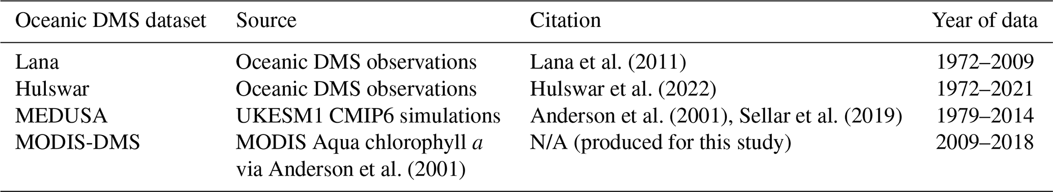
We input four oceanic DMS datasets into the model, namely three climatologies and one 10-year time series. Observational-based climatologies are from Lana et al. (2011) (hereafter “Lana”) and Hulswar et al. (2022) (“Hulswar”). The “MEDUSA” climatology (1979–2014) originates from the UKESM1 CMIP6 (Yool et al., 2021; Sellar et al., 2019; Tang et al., 2019). Table 1 outlines the oceanic DMS datasets used. Ocean biogeochemistry is simulated in the UKESM1 via MEDUSA2.0 Yool et al. (the Model of Ecosystem Dynamics, nutrient Utilization, Sequestration, and Acidification; 2020, 2013). The time series was calculated offline, using a combination of satellite data and the UKESM1 approach to calculating oceanic DMS, as described below.
In UKESM1, oceanic DMS concentrations are calculated using a diagnostic method from Anderson et al. (2001), using surface daily shortwave radiation (J), dissolved inorganic nitrogen (Q), and chl a (C) as follows:
Table 1Oceanic DMS datasets used in the model simulations. N/A stands for not applicable.
The parameter values are a=1, b=8, and s=1.56, as described by Sellar et al. (2019). Q, chl a, and J are averaged from CMIP6 for the MEDUSA climatology. The Anderson et al. (2001) parameterization produces positive biases in DMS over the Southern Ocean within MEDUSA (Bock et al., 2021), due to the set minimum oceanic concentration of 1, which leads to large average DMS concentrations (Yool et al., 2021; Bock et al., 2021). Recent research suggests that chl a may not be an appropriate proxy for oceanic DMS (Uhlig et al., 2019; Bell et al., 2021), and future work will explore alternative methods for calculating oceanic DMS within UKESM1. Nonetheless, chl a is widely used by CMIP6-era models to calculate oceanic DMS, and we explore here whether using an observationally derived chl a concentration field leads to changes in the spatial and temporal variability in the atmospheric DMS. Monthly mean chl a concentrations from the Moderate Resolution Imaging Spectroradiometer (MODIS) Aqua satellite instrument were used to construct a time series of oceanic DMS between 2009 and 2018 (Table 1; Hu et al., 2019; O'Reilly and Werdell, 2019). This time series, which we term the “MODIS-DMS” dataset, is calculated offline, using the same diagnostic parameterization as Eqs. (2) and (3). The J and Q values used to calculate MODIS-DMS remain the same as MEDUSA. Through this, we capture spatial and interannual chl a variability, indicating biological productivity. Bilinear interpolation is used to fill in small gaps (around 1 % for monthly averages) of spatial chl a data. Oceanic DMS concentrations are masked where they coincide within the sea ice zone from HadISST.
In general, the MODIS Aqua Ocean Color chl a retrieval underestimates Southern Ocean chlorophyll concentrations by up to 25 % (Zeng et al., 2016; Haëntjens et al., 2017; Jena, 2017; Gregg and Casey, 2007; Johnson et al., 2013). Simulated oceanic DMS may therefore be systematically underestimated. Nonetheless, the high spatial and temporal availability of chl a observations during summertime makes it useful to explore spatiotemporal variability in atmospheric DMS.
2.3 DMS sea-to-air flux
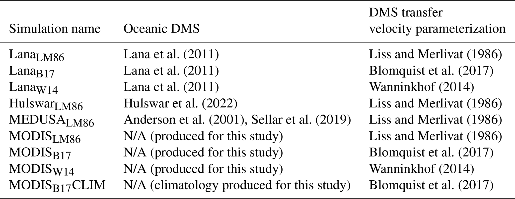
Three DMS transfer velocities are tested (Fig. 1, Table 2). Two are linear equations from Liss and Merlivat (1986) (hereafter “LM86”) and Blomquist et al. (2017) (hereafter “B17”). LM86 is a piece-wise linear equation and the default parameterization within UKESM1 (Sellar et al., 2019) and was evaluated in combination with all oceanic DMS datasets. The quadratic formula from Wanninkhof (2014) (hereafter “W14”) is also tested. Using these different parameterizations provides an appropriate estimate for the spread of DMS emissions due to the upper and lower limits of DMS transfer velocity tested from in situ DMS measurements (e.g., Goddijn-Murphy et al., 2016; Blomquist et al., 2017). Table 2 summarizes the sensitivity simulation names of simulations that were performed. Simulations are named with the oceanic DMS concentration used and subscripted with the transfer velocity used. For example, LanaLM86 means that the simulation used the Lana et al. (2011) climatology as its oceanic DMS dataset and the DMS transfer velocity parameterization of Liss and Merlivat (1986).
Lana et al. (2011)Liss and Merlivat (1986)Lana et al. (2011)Blomquist et al. (2017)Lana et al. (2011)Wanninkhof (2014)Hulswar et al. (2022)Liss and Merlivat (1986)Anderson et al. (2001)Sellar et al. (2019)Liss and Merlivat (1986)Liss and Merlivat (1986)Blomquist et al. (2017)Wanninkhof (2014)Blomquist et al. (2017)Table 2Simulations used in this study, named with the oceanic DMS concentration used and subscripted with the transfer velocity used. N/A stands for not available.
The Schmidt number for DMS is used to calculate the DMS emission. The Schmidt number represents the viscosity or diffusion properties of a gas and varies with respect to sea surface temperature (T in ∘C). We update the Schmidt number of DMS (ScDMS) used in the UKESM1 from the formulation used in Saltzman et al. (1993) to Wanninkhof (2014), as shown in Eq. (3):
where T is derived from HadISST (Titchner and Rayner, 2014). U10 (m s−1) represents near-surface (10 m) wind speed, and Kw (cm h−1) represents the transfer velocity of DMS. Equation (5) represents the LM86 transfer velocity of DMS as follows:
W14 uses a quadratic formula (Eq. 6) for sea-to-air transfer. W14 is also used to calculate DMS emissions amongst CMIP6 models from, for example, Tjiputra et al. (2020).
B17 is the only parameterization tested in this study for which the transfer velocity is based on real-world observation of DMS (Eq. 7). B17 is a super-linear parameterization; however, for simplicity and the wind speeds used in this study, we label B17 as a linear parameterization.
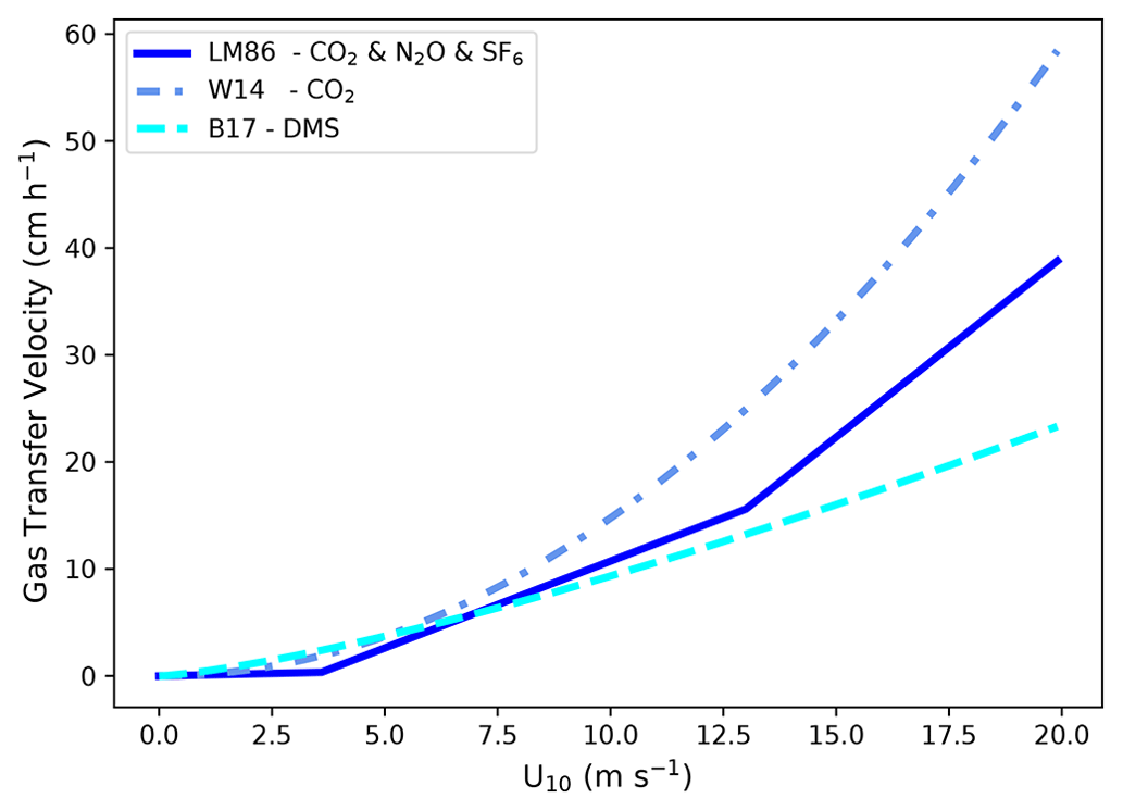
Figure 1DMS transfer velocities tested in this study. LM86 is for Liss and Merlivat (1986); W14 is for Wanninkhof (2014); and B17 is for Blomquist et al. (2017). The gases labeled in the legend are the measurements taken to identify the gas exchange relationship.
To assess the interannual variability in the DMS emissions and atmospheric DMS concentrations, we performed an additional 10-year simulation, MODISB17CLIM. While MODISB17 used a 10-year time series of oceanic DMS derived from MODIS chlorophyll a data, MODISB17CLIM used a climatology calculated from monthly mean data for the 10-year MODISB17 time series.
2.4 Observational datasets
2.4.1 Oceanic DMS and atmospheric DMS datasets
Two Southern Ocean voyages are used to evaluate our simulations, namely the SOAP campaign (Surface Ocean Aerosol Production; Bell et al., 2015; Law et al., 2017) and research vessel (R/V) Tangaroa voyage (TAN1802; Kremser et al., 2021). The SOAP voyage measured oceanic and atmospheric DMS from February–March 2012 near the Chatham Rise (within 42–47∘ S, 172–180∘ E) off the east coast of Aotearoa / New Zealand (Bell et al., 2015; Smith et al., 2018). The TAN1802 voyage measured oceanic DMS along the Southern Ocean during February–March 2018 between 40 to 70∘ S, 180∘ E (Kremser et al., 2021). We also extend the simulations to cover the ANDREXII voyage between February–April 2019 for atmospheric DMS concentrations, as this voyage mostly conducted measurements during autumn (Wohl et al., 2020). ANDREXII traveled longitudinally around 60∘ S. Although outside our simulation range, we also consider the Southern Ocean Iron RElease Experiment (SOIREE) for atmospheric DMS analysis from February 1999 (Boyd and Law, 2001) between 42–63∘ S, 139–172∘ E.
We used oceanic DMS measurements for TAN1802 Kremser et al. (2021), SOAP (Bell et al., 2015), and ERA5 surface wind speeds (Hersbach et al., 2020) to calculate hourly DMS emissions. The Wanninkhof (2014) DMS Schmidt number is calculated using the same parameters used within the simulations to ensure consistency with the comparisons to simulated fluxes. The HadISST and ERA5 wind speed data were obtained for the same time and location for both of the two voyages (within the nearest-neighbor grid cell). We applied three different transfer velocity parameterizations (LM86, B17, and W14) to both SOAP and TAN1802 voyage paths (see Sect. 3.2).
We compare our simulations to the voyage dataset using the hourly model output and identify the nearest-neighbor grid cell to the ship location. Analysis of oceanic DMS data used in the models is also synchronized to TAN1802 and SOAP voyages, using the same timescales for comparing the voyages with model data.
We also validate the model using atmospheric DMS concentrations measured at two stations, namely Kennaook / Cape Grim (1989 to 1996; 41∘ S and 145∘ E) and King Sejong Station (2018 to 2020; 62∘ S, 58∘ W). King Sejong is located on the Antarctic Peninsula, where sea ice melt occurs during our study period, which can profoundly increase DMS emissions, as previously found by Berresheim et al. (1998) and Read et al. (2008).
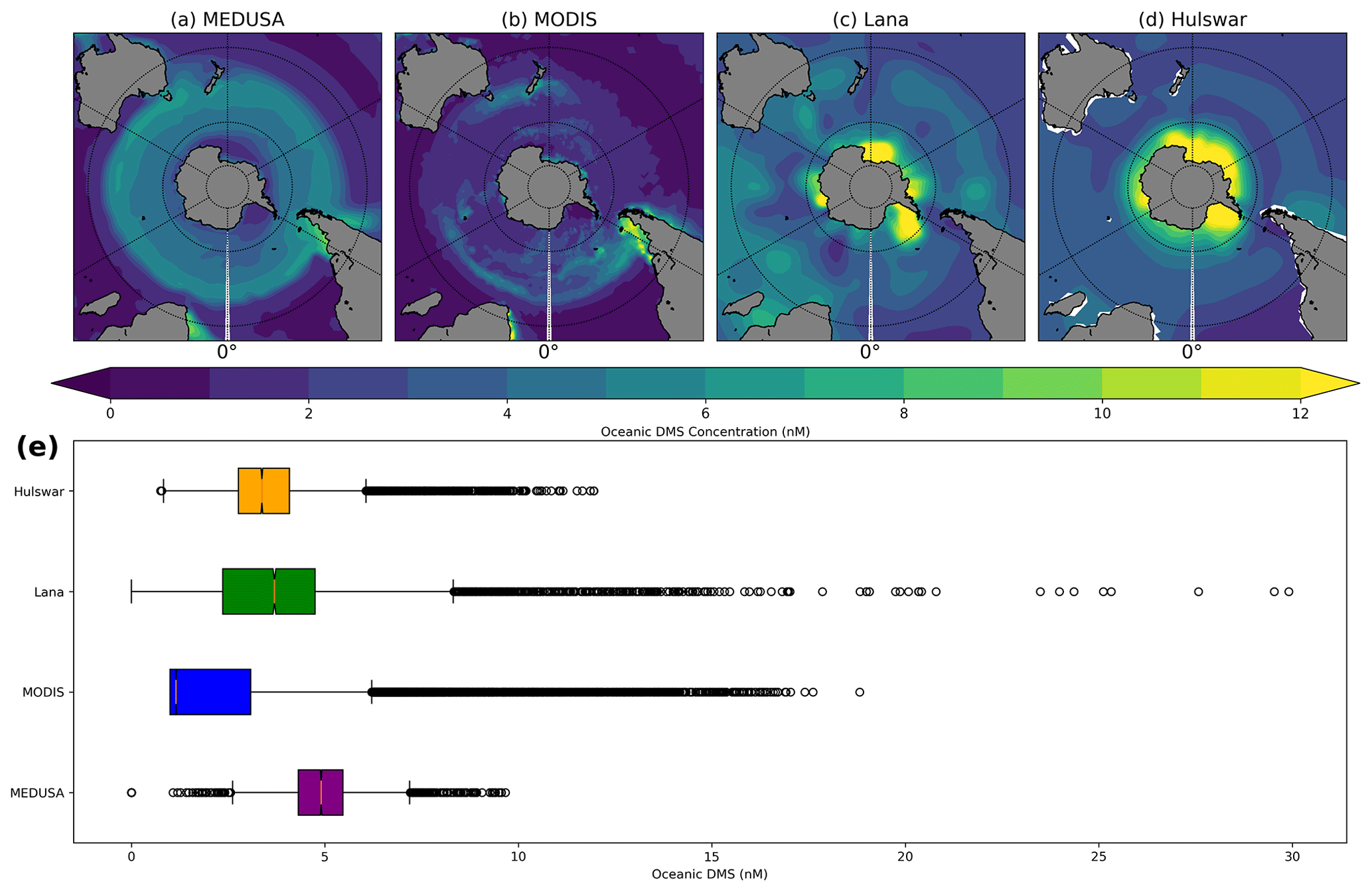
Figure 2Summertime (DJF) Oceanic DMS in the Southern Ocean (40–60 S). The spatial distribution (a–d) shows the (a) UKESM1 climatology from MEDUSA, (b) the climatology from MODIS-DMS, and observationally based climatologies of (c) Lana and (d) Hulswar. (e) The box plot shows the distribution of each oceanic DMS dataset used, where MODIS-DMS contains all 10 years of data, while the climatologies contain 12 months.
2.4.2 Cloud and aerosol observations
MODIS Aqua aerosol optical depth (AOD) measurements at 550 nm (Platnick et al., 2017) are compared with each daily mean model output. Daily averaged observations from Grosvenor et al. (2018) and Bennartz and Rausch (2017) were used to compare the cloud droplet number concentration (CDNC) with our daily averaged simulations. Finally, to evaluate cloud condensation nuclei (CCN), we used observations from Choudhury and Tesche (2023) at 818 m in comparison with simulated CCN at 800 m. The description and evaluation of using MODIS-observed AOD compared with a related configuration of UKESM1-AMIP is discussed in more detail in Revell et al. (2019) and Mulcahy et al. (2020). We calculate an austral summertime climatology for these observational datasets, which we use over the Southern Ocean.
3.1 Oceanic DMS
Figure 2a–d shows the spatial distribution of each oceanic DMS dataset. Each distribution has key defining characteristics, although Hulswar (Fig. 2d) is an update to Lana (Fig. 2c). The distinction between MODIS-DMS and MEDUSA oceanic DMS calculations is chl a, which results in distinctly different distributions, as shown in Fig. 2e. Observationally based climatologies, like Lana or Hulswar, do not align with the chl a distribution in the Southern Ocean, particularly along the Antarctic Circumpolar Current, concentrating oceanic DMS in specific regions based only on observations of oceanic DMS (Lana et al., 2011; Hulswar et al., 2022). The mean difference between the lowest (MODIS-DMS) and highest (MEDUSA) mean of all the oceanic DMS datasets used is 107 %.
MEDUSA produces the most homogeneous oceanic DMS distribution in the summertime Southern Ocean, with the highest mean and smallest standard deviation (4.88 ± 0.87 nM). It also has the lowest CoV of ± 17 %, indicating a small spread of variance. Chl a in MEDUSA shows a positive bias against summer observations in the Southern Ocean (Yool et al., 2013, 2021). In contrast, MODIS-DMS has low oceanic DMS concentrations in open-ocean regions and high concentrations in biologically productive regions (near the subtropical front), such as the Chatham Rise and coastal South America (Behrens and Bostock, 2023). MODIS-DMS has the largest spatial variability in oceanic DMS overall (CoV 67 %). The mean oceanic DMS in MODIS-DMS is 2.36 ± 1.57 nM, which is outside the range of MEDUSA, highlighting the sensitivity of the Anderson et al. (2001) parameterization to chl a concentrations.
In the MODIS-DMS simulation, oceanic DMS concentrations vary each summer across the Southern Ocean over a 10-year climatology (see Fig. S1a in the Supplement). The most significant interannual variability occurs around Aotearoa / New Zealand and South America's east coast, likely from phytoplankton blooms influenced by ENSO (Santoso et al., 2017; Thompson et al., 2015; Yoder and Kennelly, 2003; Fig. 2a). The Lana and Hulswar simulations have similar means (3.87 and 3.51 nM, respectively) but differ in their distribution (Fig. 2e). Oceanic DMS maximizes at 30 nM in Lana and at 14 nM in Hulswar. The MEDUSA simulation using the Anderson et al. (2001) parameterization shows oceanic DMS maximizing at 11 nM, while when a variable chl a concentration field is used in the MODIS-DMS simulation, oceanic DMS maximizes at 18 nM (64 % higher than in the MEDUSA simulation).
To examine how the simulations compare with observations, we compare the oceanic DMS distribution against TAN1802 and SOAP voyages for the regions and times at which those voyages took place (Figs. 3, 4). For the TAN1802 voyage (40–70∘ S, 180∘ E), the distribution of measured oceanic DMS aligns closely with the Lana simulation. MODIS-DMS and MEDUSA have lower means of 1.19 and 1.52 nM, respectively, but MODIS-DMS has a high CoV of 79 %, due to higher concentrations at lower latitudes (45∘ S) of the Southern Ocean. Oceanic DMS in the Hulswar simulation overestimates DMS concentrations by a factor of 2 between 45–65∘ S.
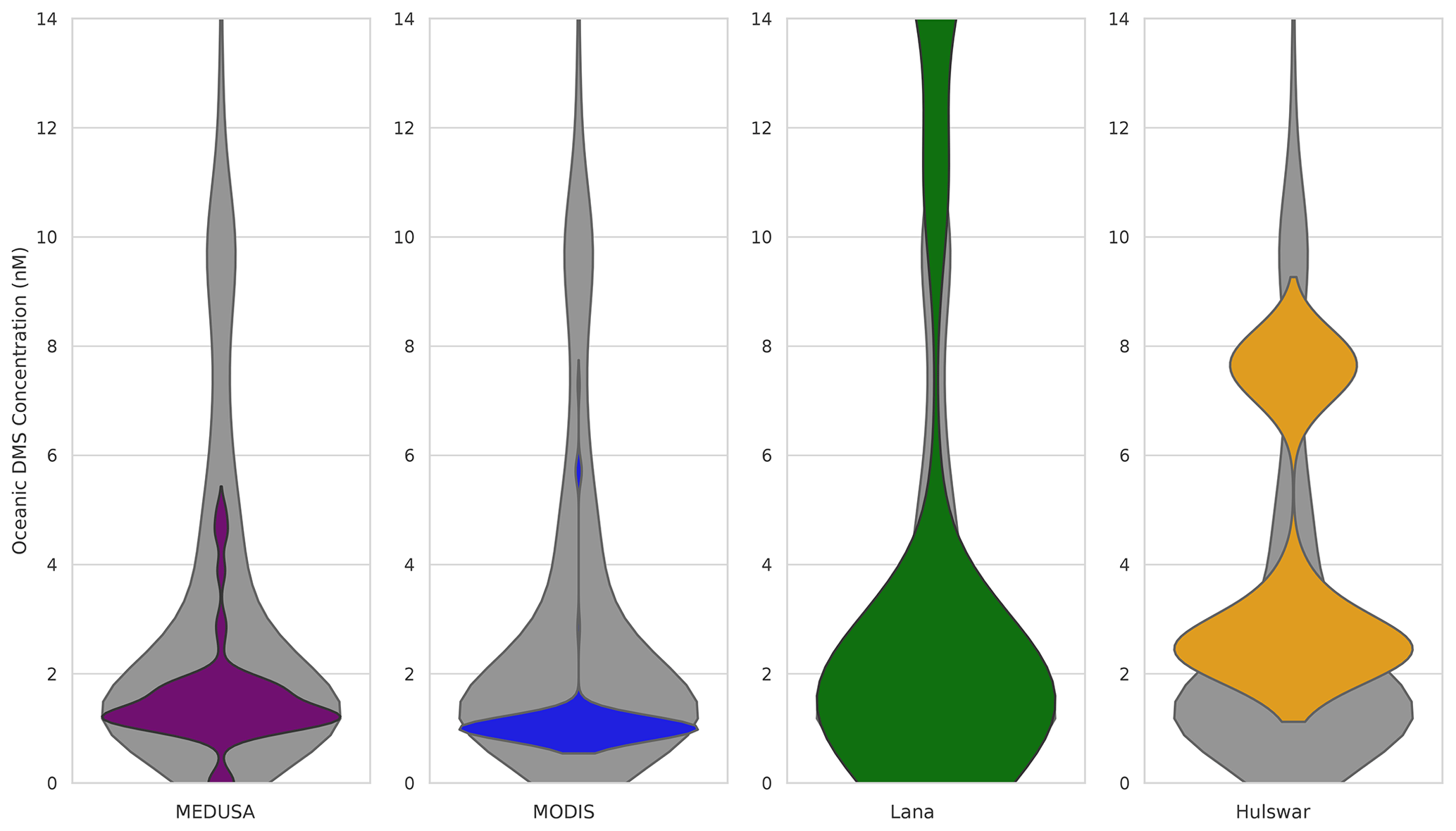
Figure 3Violin plots of TAN1802 data (gray). Overlaid are the oceanic DMS datasets used in the model simulations (February to March 2018; 40 to 70∘ S, 180∘ E) from MEDUSA (purple), MODIS-DMS (blue), Lana (green), and Hulswar (yellow). Violin plots depict data distribution and density. The width of each “violin” corresponds to the frequency of data points within that value range, while the length indicates the range of values. The frequency axis, represented by the width, allows for an immediate visual comparison of how often particular ranges of values occur in each category. This offers a comprehensive view of both the distribution and frequency of data across different categories.
For the SOAP voyage, which targeted phytoplankton bloom events (42–47∘ S, 172–180∘ E), the measured DMS distribution is skewed toward higher concentrations compared with the TAN1802 voyage (Fig. 4). In contrast, TAN1802 transected the Southern Ocean without a specific focus on bloom activity, yielding a range of DMS concentrations. We consider that SOAP is still useful, as it offers insights into extreme conditions not reflected in other datasets. All simulations fail to capture the higher concentrations measured by SOAP. Oceanic DMS in the MODIS-DMS exhibits the highest variability (CoV of 36 %), mean, and maximum concentration. MODIS-DMS also aligns best with SOAP in that it captures some of the high DMS concentrations resulting from phytoplankton blooms. The MODIS-DMS simulation captures around half of the variability in the SOAP measurements, whereas the other simulations only match between 7 % to 18 %. MODIS-DMS is within 11 % of the SOAP mean, whereas the other simulations are 22 % to 218 % lower. See Figs. S2 and S3 for simulated comparisons of DMS emission to SOAP and TAN1802.
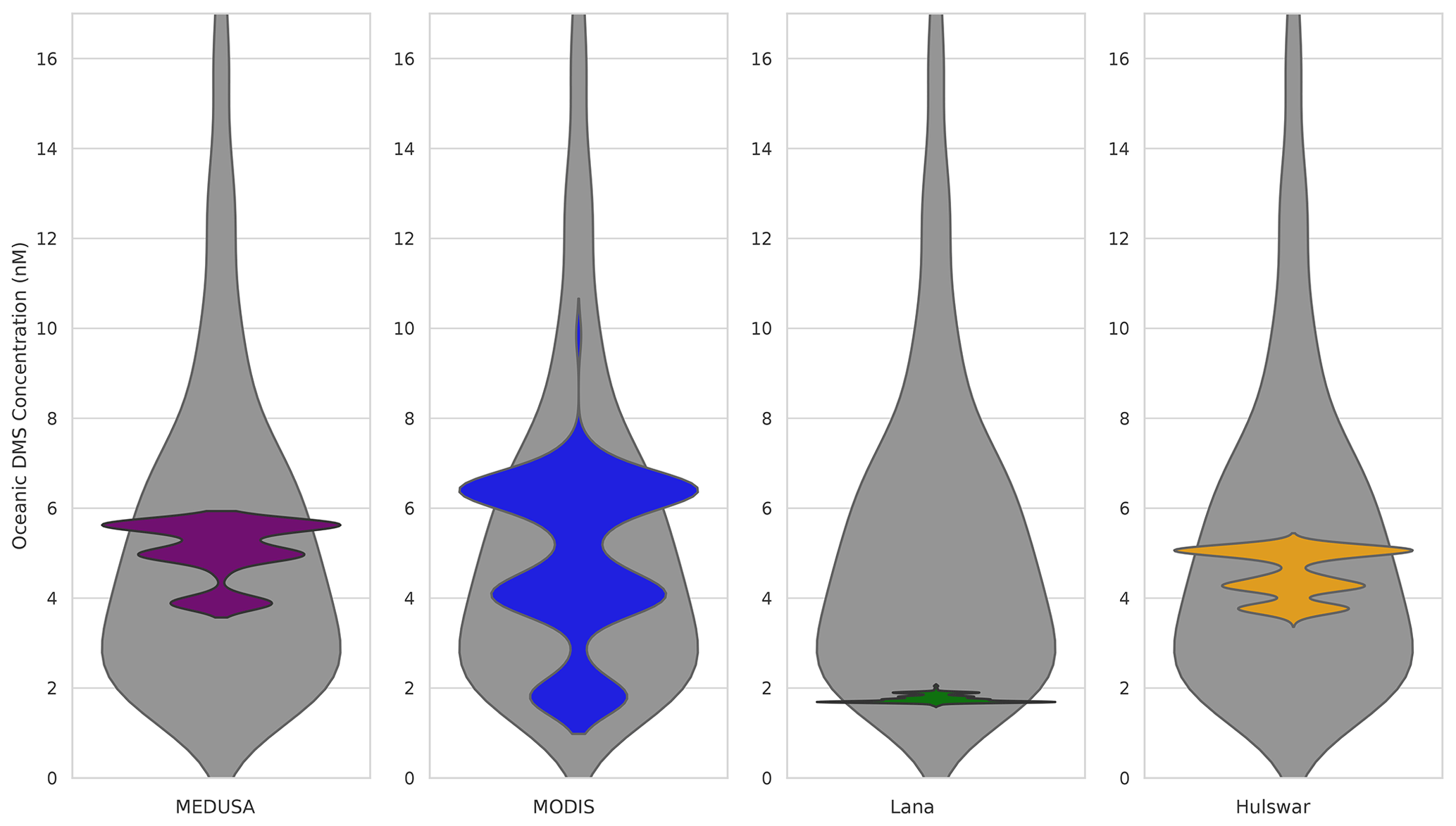
Figure 4Same as Fig. 3 but for the SOAP 2012 voyage (February to March 2012; 42–47∘ S, 172–180∘ E).
The Anderson et al. (2001) parameterization assumes chl a is central to oceanic DMS formation. Previous correlations between chl a and oceanic DMS, given by the coefficient of determination (R2), range globally from 0.11 to 0.93, with higher latitudes having increased R2 values due to factors like nutrient availability and prolonged summer daylight, coupled with heightened wind speeds (Uhlig et al., 2019; Townsend and Keller, 1996; Tison et al., 2010; Matrai et al., 1993). Gros et al. (2023) estimated an R2 of 0.93 towards sea ice latitudes, while Bell et al. (2021) found chl a explains just 15 % of oceanic DMS variability. Using the Anderson et al. (2001) parameterization in MODIS-DMS, we determined a large R2 of 0.75 in the Southern Ocean. While associating chl a with oceanic DMS has discrepancies (Gros et al., 2023; Bell et al., 2021), we show that using Anderson et al. (2001) with satellite chl a data better represents Southern Ocean summertime DMS compared with the MEDUSA configuration.
Chl a is used to calculate oceanic DMS in two of the four ESMs with interactive biogeochemistry in CMIP6 (Bock et al., 2021). These models reveal discrepancies between each other and observed oceanic DMS datasets, indicating ongoing uncertainties in CMIP6 ESMs concerning oceanic DMS and its flux to the atmosphere (Bock et al., 2021). Bock et al. (2021) emphasize the need for enhanced understanding and observations to accurately capture DMS–climate feedbacks. CNRM-ESM2-1 adopts an approach considering zooplankton and dimethylsulfoniopropionate (DMSP) rather than chl a, but its validation is challenging due to limited observational data (Belviso et al., 2012). NorESM2 uses an alternative mechanism for DMS production, by using detritus export production and sea surface temperature (Tjiputra et al., 2020). An oceanic DMS algorithm developed by Galí et al. (2018) includes sea surface temperature, chl a, photosynthetically active radiation, and the mixed-layer depth, but oceanic DMS has a general overestimation along coastal regions (Galí et al., 2019; Hayashida et al., 2020). Galí et al. (2018) also produced a time series of oceanic DMS over parts of the Northern Hemisphere, finding high interannual variability by using chl a satellite data. Adopting temporally variable oceanic DMS inputs within the model may better reflect interannual Southern Ocean variability due to ENSO events and biologically productive years. One such way to achieve this for future projections would be through a stochastic approach of capturing all chl a years from the satellite (e.g., SeaWiFS and MODIS Aqua) archive.
3.2 DMS flux
Having established that oceanic DMS from the MODIS-DMS simulation compares reasonably with summertime observational voyages, as seen in Figs. 3 and 4, we now assess the sensitivity of atmospheric DMS to various sea-to-air transfer functions (Figs. 5, S4). Figure 5 shows the DMS flux during the austral summer in the Southern Ocean, averaging between 2.9 and 7.3 TgS yr−1. This is consistent with the Jarníková and Tortell (2016) estimation of 3.4 TgS, aligning most with the MODIS-DMS linear parameterizations (LM86 and B17). The spread in average Southern Ocean summertime DMS fluxes across the eight simulations is 153 %, which is greater than the spread between all the simulations testing different oceanic DMS datasets, which is at 107 %. The lowest CoVs within both oceanic DMS and DMS emissions are found in the MODIS-DMS simulations and, specifically, the Blomquist et al. (2017) parameterization (MODISB17) with a mean of 2.9 ± 0.84 TgS yr−1. The upper range of simulated DMS flux, 7.3 ± 1.8 TgS yr−1, comes from the W14 quadratic formula used with the Lana DMS climatology (LanaW14).
The largest DMS emissions are seen in the MEDUSALM86 simulations, due to the relatively large underlying oceanic DMS values spread throughout the Southern Ocean (Fig. 2a). The Lanaw14 simulation also shows large DMS emissions due to the quadratic dependence of the gas transfer velocity on wind speed (Fig. 1). Overall, the W14 quadratic formula yields about 33 % more emissions than the LM86 and B17 linear formulas. For the transfer velocity parameterizations using a linear relationship to wind (LM86 and B17), LM86 exhibits a higher transfer velocity than B17 for wind speeds above 7.5 m s−1 (Fig. 1). Given the Southern Ocean's predominantly high wind speeds (Bracegirdle et al., 2020), simulations indicate that LM86 yields 14 % more emitted DMS than B17 (Fig. 5).
The LM86 transfer velocity parameterization was tested with all oceanic DMS datasets, as it is currently the parameterization used by default in UKESM1-AMIP. Simulations using LM86 have a spread in the average summertime Southern Ocean DMS emissions of 112 % (3.3 to 6.9 TgS yr−1). In contrast, simulations using the same oceanic DMS dataset (MODIS-DMS and Lana) but including transfer velocity parameterizations (LM86, B17, and W14) have a spread in the average summertime Southern Ocean DMS emissions from 51 % (MODIS-DMS simulations) to 62 % (Lana simulations). The choice of the oceanic DMS dataset therefore impacts DMS emissions more than the transfer velocity parameterization within these simulations.
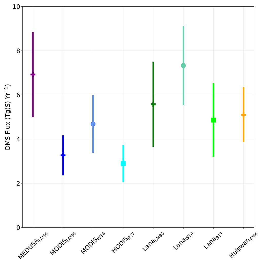
Figure 5Summertime (December–February) Southern Ocean sulfur emissions in teragrams per year (Tg yr−1) in all model simulations performed. The error bars represent the spatiotemporal standard deviation. The different colors represent different oceanic DMS climatologies. Purple refers to MEDUSA (Sellar et al., 2019; Anderson et al., 2001); green (Lana et al., 2011) and orange refer to Hulswar (Hulswar et al., 2022), and the time series in blue is derived from MODIS-DMS chl a, which is used in this work. The plus (+) marker represents simulations performed with the Liss and Merlivat (1986) sea-to-air flux, the dot marker represents Wanninkhof (2014), and the square marker represents Blomquist et al. (2017).
Many CMIP6 models use the quadratic transfer velocity parameterization detailed in Wanninkhof (2014) for DMS emissions (e.g., Salzmann et al., 2022; Seland et al., 2019; Neubauer et al., 2019; Tatebe and Watanabe, 2018; Wu et al., 2019). Yet, recent studies indicate a linear relationship between DMS and wind speed (e.g., Blomquist et al., 2017; Yang et al., 2011; Bell et al., 2013, 2015). We demonstrate that linear DMS transfer velocities represent the DMS flux ranges better than the quadratic W14 flux when compared to Southern Ocean observations.
3.3 Atmospheric DMS
We next evaluate atmospheric DMS in our sensitivity simulations. Figure 6 compares all simulated atmospheric DMS with the observational datasets. Data in Fig. 6 are from three Southern Ocean voyages (SOAP, SOIREE, and ANDREXII; Fig. 6a–c) and two stations (Kennaook / Cape Grim and King Sejong Station; Fig. 6d–e). Figure 6f shows the aggregate-averaged DMS concentrations from all five observational sources and has an average summertime concentration of 129 ± 74 ppt (parts per trillion) (Fig. 6f; Smith et al., 2018; Wohl et al., 2020; Boyd and Law, 2001). The simulations using the MODIS-DMS oceanic dataset and linear DMS transfer models (LM86 and B17) show the closest agreement with the observational mean of 106 ± 66 ppt and 100 ± 60 ppt for MODISLM86 and MODISB17, respectively. The mean total spread in the summertime Southern Ocean atmospheric DMS across all simulations is 171 %, compared with the spread of 153 % in DMS emissions.
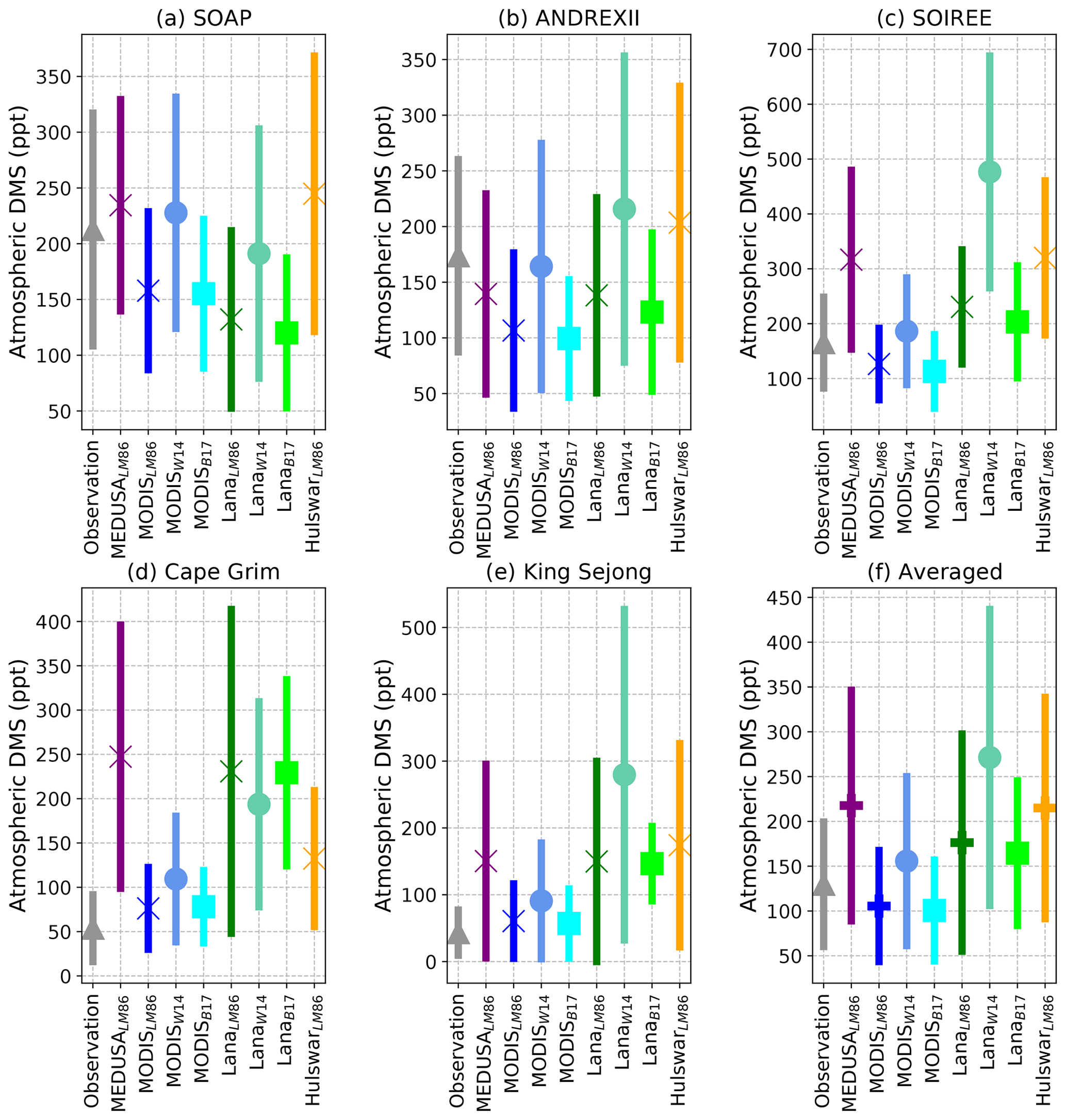
Figure 6Five observational datasets measuring atmospheric DMS concentrations (ppt) are directly compared with the eight simulations (a–e) at the same spatial and temporal resolution. For (a) SOAP and (b) ANDREXII, we follow both voyages using the nearest-neighbor grid cell along each hour of the simulations, matching the timescales in 2012 and 2019. For comparing the simulations with the (c) SOIREE voyage, we also follow this voyage on an hourly timescale, but due to the voyage being outside our study period, we average this over all 10 years. The two observational stations used are (d) Kennaook / Cape Grim and (e) King Sejong Station. We calculate the nearest-neighbor grid cell for each simulation to the observational station and constructed an average over 10 years, along with a temporal standard deviation. From this, we construct an overall average (f) and standard deviation for all observational measurements and simulations, which can be compared directly to these observations.
Our simulations, compared to coastal Antarctic measurements, offer insights into the performance of sea-ice-influenced regions (Galí et al., 2021). In summer, Berresheim et al. (1998) recorded mean atmospheric DMS of 119 ppt at 64.8∘ S, 64∘ W, closely matching MODISB17 at 121 ppt. All other oceanic DMS datasets show concentrations which are more than twice as large as this measurement. Read et al. (2008) measured atmospheric DMS concentrations of 45 ± 50 ppt at Halley VI Research Station, Antarctica (75.4∘ S, 26.2∘ W), best aligning with LanaB17 at 42 ppt. It should be noted that all simulations fall within 1 standard deviation of the measurements reported at Halley Station. Preunkert et al. (2007) measured high interannual variation in the atmospheric DMS at Dumont d'Urville Station (66.4∘ S, 140∘ E) during January, from 244 ppt in 2002 to only 60 ppt in 2003. The average January concentration over 13 years was 170 ± 180 ppt. Here, the Lana and Hulswar simulations are in closest agreement and simulate average DMS concentrations between 92 and 141 ppt. Last, Lee et al. (2010) measured a 61 ppt average over the Pacific–Southern Ocean in February, closest to MODISB17 and MODISLM86 (64 and 53 ppt, respectively).
Multiannual studies emphasize high yearly variability (Read et al., 2008; Preunkert et al., 2007). Measurements during austral summer over the Southern Ocean show significant variability, especially in higher latitudes. The climatologies produce higher concentrations along the coastal regions of Antarctica, as illustrated in Fig. 2a–d, but MODIS-DMS still captures much of the spatial variability (Fig. S5). MEDUSA performs the worst over these higher-latitude regions, where sea ice can have a large role in producing atmospheric DMS (Galí et al., 2021). MODISB17 represents atmospheric DMS more accurately than models like MEDUSA, Lana, and Hulswar, based on observations over the Southern Ocean during summertime.
3.4 Effects from interannual and spatial variability
To assess the impact of interannual variability in oceanic DMS on simulated atmospheric DMS, we compare the MODISB17 simulation with MODISB17CLIM, which used a climatology of oceanic DMS calculated from the MODIS-DMS dataset (Fig. 7). Both simulations are similar (R2=0.92) in terms of interannual variability across the Southern Ocean as a whole (Fig. 7c). Rolling means are presented in Fig. S1b and c. While there are small differences in Southern Ocean atmospheric DMS between the simulations, the overwhelming similarities between Fig. 7a and b suggest that an oceanic DMS climatology results in similar interannual variability in the atmospheric DMS probability density function (PDF), suggesting that oceanic DMS is not a strong driver of interannual variability in atmospheric DMS. This result is in contrast to that of Galí et al. (2018), who used a different algorithm for producing oceanic DMS. This difference may be due to our use of the Anderson et al. (2001) algorithm, which is known to produce limited variability (Belviso et al., 2004; Bock et al., 2021).
To assess the impact of spatial variability in oceanic DMS on simulated atmospheric DMS, we compare simulations performed using the MEDUSA and MODIS-DMS datasets (with low and high spatial variability in oceanic DMS, respectively) in Fig. 8. The larger variability in the MODIS-DMS oceanic DMS dataset leads to larger variability in simulated atmospheric DMS when compared with the MEDUSA simulations. The spatial CoV from MEDUSALM86 is 45 % lower than MODISLM86, showing greater spatial variability from MODIS-derived chl a. The oceanic DMS signal in the atmosphere is strong but includes large fluctuations driven by the wind variations.
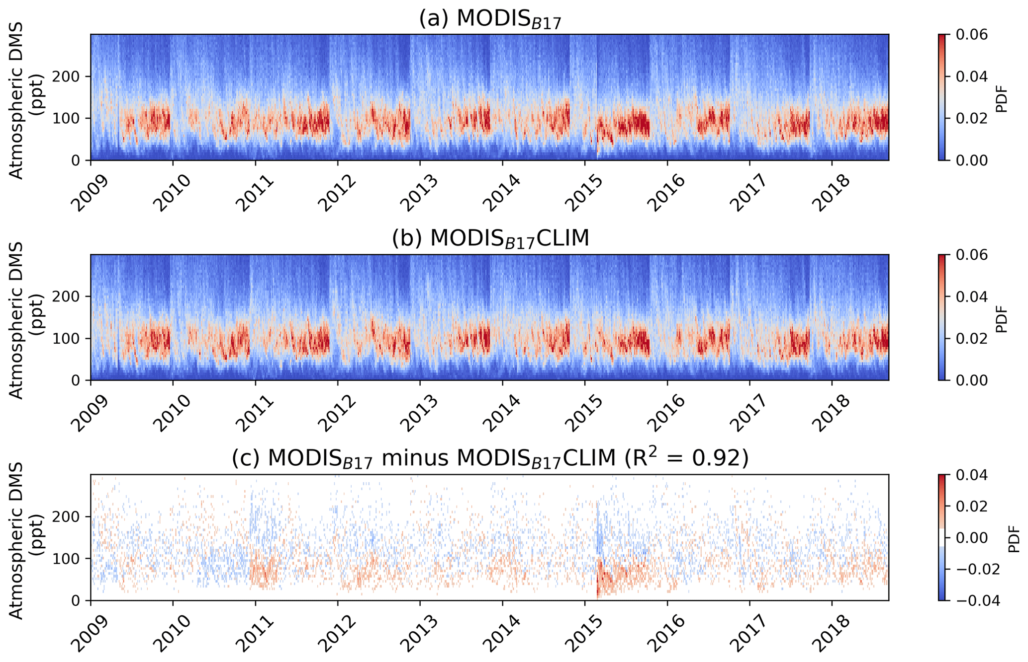
Figure 7Time series of the atmospheric DMS probability density function between (a) MODISB17 and (b) MODISB17CLIM from 2009 to 2018 summer over the entire Southern Ocean. (c) The difference between MODISB17 and MODISB17CLIM is also shown, with the R2 shown between the two simulations.
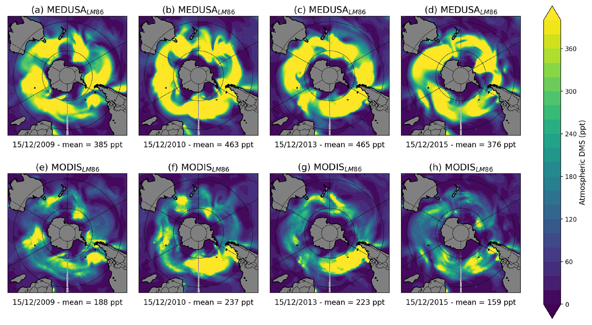
Figure 8Atmospheric DMS concentrations comparing (a–d) MEDUSALM86 with (e–h) MODISLM86 across 4 of the same summertime days (15 December) in (a, e) 2009, (b, f) 2010, (c, g) 2013, and (d, h) 2015. The area-weighted Southern Ocean mean is shown below each plot.
3.5 Aerosol and cloud response
Figures 9 and S6 show the effect on cloud and aerosol properties of changing the atmospheric DMS distribution. Changing the atmospheric DMS concentration yields a spread across all our simulations for AOD, CDNC, and CCN by 6 %, 15 %, and 11 %, respectively, over the austral summer Southern Ocean. As DMS predominately oxidizes into sulfate within the smaller aerosol modes, it has a smaller influence on the AOD than the larger modes from sea salt aerosol (Mulcahy et al., 2020). However, these smaller aerosols influence cloud seeding, as our simulations show. Changes to the oceanic DMS dataset increase the spread in simulated CCN and CDNC over the Southern Ocean rather than changing the DMS emissions, which is consistent with our findings for atmospheric DMS concentrations. Altering the oceanic DMS dataset produces a 73 % greater change in AOD than altering the DMS emissions over the Southern Ocean, emphasizing the role of the ocean in producing atmospheric DMS. Box plots of AOD, CCN, and CDNC (Fig. 9e, a, c) show that the simulations do not capture the maxima in CDNC, CCN, or AOD over the Southern Ocean.
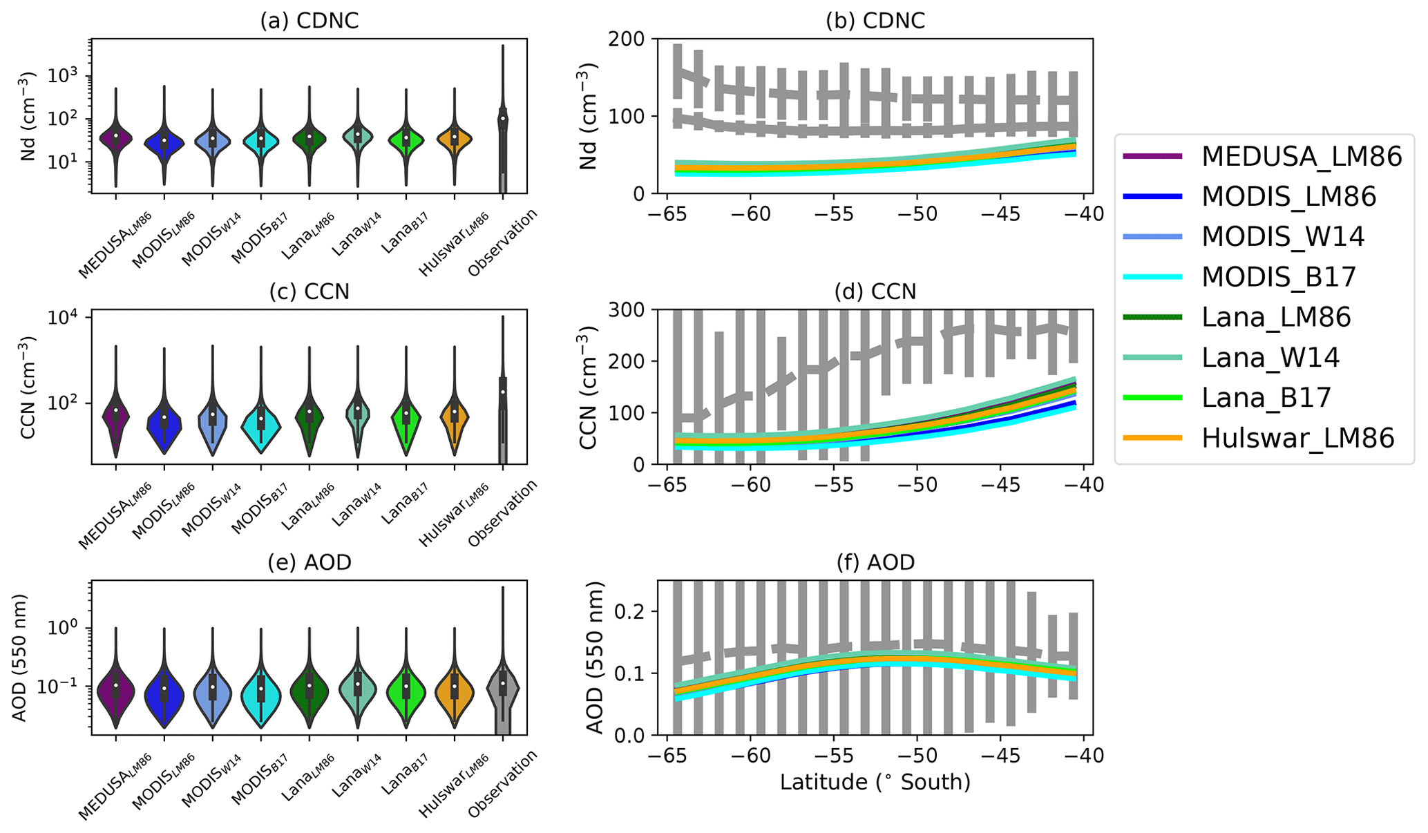
Figure 9Summertime climatology between 60 to 40∘ S showing the (a, b) cloud droplet number concentrations, (c, d) cloud conversation nuclei (800 m in altitude), and (d, e) aerosol optical depth at 550 nm. The violin plots (a, c, e) represent all spatial and temporal data points across the 10 years over the Southern Ocean in December–February (DJF). The lowest 1 % of values are excluded from the violin plots. (b, d, f) The gray lines represent observational datasets, where (b) Grosvenor et al. (2018) (dashed) and Bennartz and Rausch (2017) (solid) are shown for CDNC. (d) Choudhury and Tesche (2023) is shown at 818 m. (f) AOD climatology by the MODIS satellite retrieval is shown (Platnick et al., 2017). The error bars represent 1 standard deviation on either side of the observational mean.
We examined the sensitivity of atmospheric DMS to different oceanic DMS datasets and transfer velocity parameterizations using the UKESM1-AMIP model. Modeled atmospheric DMS over the Southern Ocean is sensitive to both oceanic DMS concentrations and sea-to-air emissions. The current approach to calculating oceanic DMS within UKESM1 (MEDUSA; Anderson et al., 2001) shows little spatial variability and high average biases in the Southern Ocean region, emphasizing the need for further refinement (e.g., Bock et al., 2021; Mulcahy et al., 2020; Yool et al., 2021). Incorporating satellite chlorophyll a observations within the Anderson et al. (2001) oceanic DMS parameterization produces larger spatial variability than MEDUSA. MODIS-DMS simulations indicate that large open-water areas in the Southern Ocean have lower oceanic DMS concentrations compared to the other three oceanic DMS datasets tested (MEDUSA, Lana, and Hulswar). Lana and Hulswar, compiled from in situ observations, depict fewer distinct features in oceanic DMS concentrations than MODIS-DMS, including along coastal regions and at higher latitudes.
Current oceanic DMS climatologies in climate models lack similar spatial distribution to ocean chlorophyll a during Southern Ocean summer and perform poorly relative to observations from voyages and atmospheric DMS comparisons. We show how using chlorophyll a data from the MODIS Aqua satellites offers an alternative spatial representation of oceanic DMS based on the chlorophyll a distribution. Approaches like this, and that of Galí et al. (2018), offer promising avenues for realistically capturing spatial variability in oceanic DMS associated with marine biogenic activity.
During the austral summer over the Southern Ocean, the Wanninkhof (2014) quadratic DMS parameterization leads to 33 % more DMS emissions than the Liss and Merlivat (1986) and Blomquist et al. (2017) parameterizations. Linear transfer velocity parameterizations also align better with observations for DMS emissions, particularly for the MODIS-DMS simulations.
Atmospheric DMS in the 10-year MODIS-DMS time series simulation shows similar interannual variability to the climatology simulation. We show that capturing large-scale spatial variability is more important for oceanic DMS concentrations than capturing large-scale interannual variability.
In simulations with different oceanic DMS datasets but the same transfer velocity parameterization, the Southern Ocean summertime DMS emissions vary by 112 % (3.3 to 6.9 TgS yr−1). This is approximately twice as much as the simulations using the same oceanic DMS dataset, but different transfer velocity parameterizations, in which DMS emissions vary by 50 %–60 % (2.9 to 4.7 TgS yr−1). The choice of oceanic DMS dataset therefore has a larger influence on atmospheric DMS than the choice of DMS transfer velocity. The total spread in average Southern Ocean DMS emissions across all simulations is 153 %. Both oceanic DMS and DMS transfer velocity parameterization changes significantly influence atmospheric DMS, emphasizing the need for careful consideration in future research. Changing the oceanic DMS concentrations and transfer velocity results in a mean spread between the simulations of 6 % for AOD and 15 % for CDNC.
Future work will adopt more recent parameterizations of oceanic DMS concentrations and test various sulfate chemistry schemes. In future, we recommend that models use up-to-date transfer velocity parameterizations specific to DMS, such as Blomquist et al. (2017).
CDNC observations are available from Grosvenor et al. (2018) and Gryspeerdt et al. (2022) (https://doi.org/10.5194/amt-15-3875-2022). MODIS AOD and chlorophyll a observations were accessed via the Giovanni online data system, which is developed and maintained by the NASA Goddard Earth Sciences Data and Information Services Center (GES DISC; https://giovanni.gsfc.nasa.gov/, Platnick et al., 2015). DMS measurements from Amsterdam Island were obtained from the World Data Centre of Greenhouse Gases at https://ebas-data.nilu.no/ (EBAS, 2023). TAN1802 measurements are available from Kremser et al. (2021). DMS measurements from the SOIREE campaign are available from Boyd (2009) (http://lod.bco-dmo.org/id/dataset/3212). For the ANDREXII DMS datasets, see Wohl et al. (2020).
Model simulation data are archived at the Aotearoa / New Zealand eScience Infrastructure (https://www.nesi.org.nz/, NeSI, 2023) and are available by contacting the corresponding author.
The supplement related to this article is available online at: https://doi.org/10.5194/acp-23-15181-2023-supplement.
YAB implemented model developments, performed model simulations, and wrote the article, with assistance from all co-authors. LER, AJM, and AJS assisted with the experimental design and the model evaluation by comparing with the observational datasets and sensitivity analysis. ATA advised on DMS chemistry and aerosols over the Southern Ocean. CH provided assistance for lodging DMS emissions into the UKESM1 trunk. JW and EB provided technical expertise in running the model simulations.
The contact author has declared that none of the authors has any competing interests.
Publisher’s note: Copernicus Publications remains neutral with regard to jurisdictional claims made in the text, published maps, institutional affiliations, or any other geographical representation in this paper. While Copernicus Publications makes every effort to include appropriate place names, the final responsibility lies with the authors.
This research has been supported by the Deep South National Science Challenge (grant nos. C01X141E2 and C01X1901) and the UK Met Office for the use of the MetUM. We also acknowledge the contribution of Aotearoa / New Zealand eScience Infrastructure (NeSI) high-performance computing facilities to the results of this research. Aotearoa / New Zealand's national facilities are provided by NeSI and funded jointly by NeSI's collaborator institutions and through the Ministry of Business, Innovation and Employment's Research Infrastructure program (https://www.nesi.org.nz/, last access: 6 April 2023). We acknowledge the Cape Grim Science Program for the provision of DMS data from Kennaook / Cape Grim. The Cape Grim Science Program is a collaboration between the Australian Bureau of Meteorology and CSIRO Australia. Laura E. Revell appreciates support by the Rutherford Discovery Fellowships funded by the Aotearoa / New Zealand government, administered by the Royal Society Te Apārangi.
Deep South National Science Challenge (grant nos. C01X141E2 and C01X1901).
This paper was edited by Rebecca Garland and reviewed by Hakase Hayashida and Mingxi Yang.
Anderson, T., Spall, S., Yool, A., Cipollini, P., Challenor, P., and Fasham, M.: Global fields of sea surface dimethylsulfide predicted from chlorophyll, nutrients and light, J. Mar. Syst., 30, 1–20, https://doi.org/10.1016/S0924-7963(01)00028-8, 2001. a, b, c, d, e, f, g, h, i, j, k, l, m, n, o, p, q
Bates, T. S., Cline, J. D., Gammon, R. H., and Kelly-Hansen, S. R.: Regional and seasonal variations in the flux of oceanic dimethylsulfide to the atmosphere, J. Geophys. Res.-Oceans, 92, 2930–2938, 1987. a
Behrens, E. and Bostock, H.: The Response of the Subtropical Front to Changes in the Southern Hemisphere Westerly Winds—Evidence From Models and Observations, J. Geophys. Res.-Oceans, 128, e2022JC019139, https://doi.org/10.1029/2022JC019139, 2023. a
Bell, T. G., De Bruyn, W., Miller, S. D., Ward, B., Christensen, K. H., and Saltzman, E. S.: Air–sea dimethylsulfide (DMS) gas transfer in the North Atlantic: evidence for limited interfacial gas exchange at high wind speed, Atmos. Chem. Phys., 13, 11073–11087, https://doi.org/10.5194/acp-13-11073-2013, 2013. a
Bell, T. G., De Bruyn, W., Marandino, C. A., Miller, S. D., Law, C. S., Smith, M. J., and Saltzman, E. S.: Dimethylsulfide gas transfer coefficients from algal blooms in the Southern Ocean, Atmos. Chem. Phys., 15, 1783–1794, https://doi.org/10.5194/acp-15-1783-2015, 2015. a, b, c, d, e
Bell, T. G., Porter, J. G., Wang, W.-L., Lawler, M. J., Boss, E., Behrenfeld, M. J., and Saltzman, E. S.: Predictability of Seawater DMS During the North Atlantic Aerosol and Marine Ecosystem Study (NAAMES), Front. Mar. Sci., 7, 596763, https://doi.org/10.3389/fmars.2020.596763, 2021. a, b, c
Belviso, S., Bopp, L., Moulin, C., Orr, J. C., Anderson, T., Aumont, O., Chu, S., Elliott, S., Maltrud, M. E., and Simó, R.: Comparison of global climatological maps of sea surface dimethyl sulfide, Global Biogeochem. Cy., 18, 3, https://doi.org/10.1029/2003GB002193, 2004. a
Belviso, S., Masotti, I., Tagliabue, A., Bopp, L., Brockmann, P., Fichot, C., Caniaux, G., Prieur, L., Ras, J., Uitz, J., Loisel, H., Dessailly, D., Alvain, S., Kasamatsu, N., and Fukuchi, M.: DMS dynamics in the most oligotrophic subtropical zones of the global ocean, Biogeochemistry, 110, 215–241, https://doi.org/10.1007/s10533-011-9648-1, 2012. a
Bennartz, R. and Rausch, J.: Global and regional estimates of warm cloud droplet number concentration based on 13 years of AQUA-MODIS observations, Atmos. Chem. Phys., 17, 9815–9836, https://doi.org/10.5194/acp-17-9815-2017, 2017. a, b
Berresheim, H., Huey, J., Thorn, R., Eisele, F., Tanner, D., and Jefferson, A.: Measurements of dimethyl sulfide, dimethyl sulfoxide, dimethyl sulfone, and aerosol ions at Palmer Station, Antarctica, J. Geophys. Res.-Atmos., 103, 1629–1637, 1998. a, b
Bhatti, Y. A., Revell, L. E., and McDonald, A. J.: Influences of Antarctic ozone depletion on Southern Ocean aerosols, J. Geophys. Res.-Atmos., 127, e2022JD037199, https://doi.org/10.1029/2022JD037199, 2022. a
Blomquist, B. W., Brumer, S. E., Fairall, C. W., Huebert, B. J., Zappa, C. J., Brooks, I. M., Yang, M., Bariteau, L., Prytherch, J., Hare, J. E., and others: Wind speed and sea state dependencies of air-sea gas transfer: Results from the High Wind speed Gas exchange Study (HiWinGS), J. Geophys. Res.-Oceans, 122, 8034–8062, 2017. a, b, c, d, e, f, g, h, i, j, k, l, m
Bock, J., Michou, M., Nabat, P., Abe, M., Mulcahy, J. P., Olivié, D. J. L., Schwinger, J., Suntharalingam, P., Tjiputra, J., van Hulten, M., Watanabe, M., Yool, A., and Séférian, R.: Evaluation of ocean dimethylsulfide concentration and emission in CMIP6 models, Biogeosciences, 18, 3823–3860, https://doi.org/10.5194/bg-18-3823-2021, 2021. a, b, c, d, e, f, g, h, i, j, k
Boyd, P. W.: Cruise data inventory from the R/V Tangaroa 61TG_3052 cruise in the Southern Ocean during 1999 (SOIREE project), Biological and Chemical Oceanography Data Management Office (BCO-DMO) [data set], (Version 17 Sept 2009) Version Date: 17 September 2009, http://lod.bco-dmo.org/id/dataset/3212 (last access: 4 December 2019), 2009. a
Boyd, P. W. and Law, C. S.: The Southern Ocean Iron RElease Experiment (SOIREE) - introduction and summary, Deep Sea Res. Part II, 48, 2425–2438, https://doi.org/10.1016/S0967-0645(01)00002-9, 2001. a, b
Bracegirdle, T., Holmes, C., Hosking, J., Marshall, G., Osman, M., Patterson, M., and Rackow, T.: Improvements in circumpolar Southern Hemisphere extratropical atmospheric circulation in CMIP6 compared to CMIP5, Earth Space Sci., 7, e2019EA001065, https://doi.org/10.1029/2019EA001065, 2020. a
Browning, T. J., Stone, K., Bouman, H. A., Mather, T. A., Pyle, D. M., Moore, C. M., and Martinez-Vicente, V.: Volcanic ash supply to the surface ocean—remote sensing of biological responses and their wider biogeochemical significance, Front. Mar. Sci., 2, 14, https://doi.org/10.3389/fmars.2015.00014, 2015. a
Choudhury, G. and Tesche, M.: A first global height-resolved cloud condensation nuclei data set derived from spaceborne lidar measurements, Earth Syst. Sci. Data, 15, 3747–3760, https://doi.org/10.5194/essd-15-3747-2023, 2023. a, b
Curson, A. R. J., Todd, J. D., Sullivan, M. J., and Johnston, A. W. B.: Catabolism of dimethylsulphoniopropionate: microorganisms, enzymes and genes, Nat. Rev. Microbiol., 9, 849–859, https://doi.org/10.1038/nrmicro2653, 2011. a
Deppeler, S. L. and Davidson, A. T.: Southern Ocean phytoplankton in a changing climate, Front. Mar. Sci., 4, 40, https://doi.org/10.3389/fmars.2017.00040, 2017. a, b, c
EBAS: Convention on Long-Range Transboundary Air Pollution, United Nations Economic Commission for Europe. EBAS Database EMEP Framework – European Monitoring and Evaluation Programme PM2.5 and PM10 Data 1999–2014, https://ebas-data.nilu.no/ (last access: 17 May 2023), 2023. a
Elliott, S.: Dependence of DMS global sea-air flux distribution on transfer velocity and concentration field type, J. Geophys. Res.-Biogeosci., 114, 2156–2202, https://doi.org/10.1029/2008JG000710, 2009. a
Fairall, C., Yang, M., Bariteau, L., Edson, J., Helmig, D., McGillis, W., Pezoa, S., Hare, J., Huebert, B., and Blomquist, B.: Implementation of the Coupled Ocean-Atmosphere Response Experiment flux algorithm with CO2, dimethyl sulfide, and O3, J. Geophys. Res.-Oceans, 116, C4, https://doi.org/10.1029/2010JC006884 , 2011. a
Galí, M., Levasseur, M., Devred, E., Simó, R., and Babin, M.: Sea-surface dimethylsulfide (DMS) concentration from satellite data at global and regional scales, Biogeosciences, 15, 3497–3519, https://doi.org/10.5194/bg-15-3497-2018, 2018. a, b, c, d, e
Galí, M., Devred, E., Babin, M., and Levasseur, M.: Decadal increase in Arctic dimethylsulfide emission, P. Natl. Acad. Sci. USA, 116, 19311–19317, 2019. a
Galí, M., Lizotte, M., Kieber, D. J., Randelhoff, A., Hussherr, R., Xue, L., Dinasquet, J., Babin, M., Rehm, E., and Levasseur, M.: DMS emissions from the Arctic marginal ice zone, Elem. Sci. Anth., 9, 00113, https://doi.org/10.1525/elementa.2020.00113, 2021. a, b
Goddijn-Murphy, L., Woolf, D. K., Callaghan, A. H., Nightingale, P. D., and Shutler, J. D.: A reconciliation of empirical and mechanistic models of the air-sea gas transfer velocity, J. Geophys. Res.-Oceans, 121, 818–835, 2016. a, b
Gregg, W. W. and Casey, N. W.: Sampling biases in MODIS and SeaWiFS ocean chlorophyll data, Remote Sens. Environ., 111, 25–35, 2007. a
Gros, V., Bonsang, B., Sarda-Estève, R., Nikolopoulos, A., Metfies, K., Wietz, M., and Peeken, I.: Concentrations of dissolved dimethyl sulfide (DMS), methanethiol and other trace gases in context of microbial communities from the temperate Atlantic to the Arctic Ocean, Biogeosciences, 20, 851–867, https://doi.org/10.5194/bg-20-851-2023, 2023. a, b
Grosvenor, D. P., Sourdeval, O., Zuidema, P., Ackerman, A., Alexandrov, M. D., Bennartz, R., Boers, R., Cairns, B., Chiu, J. C., Christensen, M., Deneke, H., Diamond, M., Feingold, G., Fridlind, A., Hünerbein, A., Knist, C., Kollias, P., Marshak, A., McCoy, D., Merk, D., Painemal, D., Rausch, J., Rosenfeld, D., Russchenberg, H., Seifert, P., Sinclair, K., Stier, P., van Diedenhoven, B., Wendisch, M., Werner, F., Wood, R., Zhang, Z., and Quaas, J.: Remote Sensing of Droplet Number Concentration in Warm Clouds: A Review of the Current State of Knowledge and Perspectives, Rev. Geophys., 56, 409–453, https://doi.org/10.1029/2017RG000593, 2018. a, b, c
Gryspeerdt, E., McCoy, D. T., Crosbie, E., Moore, R. H., Nott, G. J., Painemal, D., Small-Griswold, J., Sorooshian, A., and Ziemba, L.: The impact of sampling strategy on the cloud droplet number concentration estimated from satellite data, Atmos. Meas. Tech., 15, 3875–3892, https://doi.org/10.5194/amt-15-3875-2022, 2022. a
Hajima, T., Watanabe, M., Yamamoto, A., Tatebe, H., Noguchi, M. A., Abe, M., Ohgaito, R., Ito, A., Yamazaki, D., Okajima, H., Ito, A., Takata, K., Ogochi, K., Watanabe, S., and Kawamiya, M.: Development of the MIROC-ES2L Earth system model and the evaluation of biogeochemical processes and feedbacks, Geosci. Model Dev., 13, 2197–2244, https://doi.org/10.5194/gmd-13-2197-2020, 2020. a
Hayashida, H., Carnat, G., Galí, M., Monahan, A. H., Mortenson, E., Sou, T., and Steiner, N. S.: Spatiotemporal variability in modeled bottom ice and sea surface dimethylsulfide concentrations and fluxes in the Arctic during 1979–2015, Global Biogeochem. Cy., 34, e2019GB006456, https://doi.org/10.1029/2019GB006456, 2020. a
Haëntjens, N., Boss, E., and Talley, L. D.: Revisiting O cean C olor algorithms for chlorophyll a and particulate organic carbon in the S outhern O cean using biogeochemical floats, J. Geophys. Res.-Oceans, 122, 6583–6593, 2017. a
Hersbach, H., Bell, B., Berrisford, P., Hirahara, S., Horányi, A., Muñoz-Sabater, J., Nicolas, J., Peubey, C., Radu, R., Schepers, D., and others: The ERA5 global reanalysis, Q. J. Roy. Meteor. Soc., 146, 1999–2049, 2020. a, b
Hu, C., Feng, L., Lee, Z., Franz, B. A., Bailey, S. W., Werdell, P. J., and Proctor, C. W.: Improving satellite global chlorophyll a data products through algorithm refinement and data recovery, J. Geophys. Res.-Oceans, 124, 1524–1543, 2019. a
Huebert, B. J., Blomquist, B. W., Yang, M. X., Archer, S. D., Nightingale, P. D., Yelland, M. J., Stephens, J., Pascal, R. W., and Moat, B. I.: Linearity of DMS transfer coefficient with both friction velocity and wind speed in the moderate wind speed range, Geophys. Res. Lett., 37, 1, https://doi.org/10.1029/2009GL041203, 2010. a
Hulswar, S., Simó, R., Galí, M., Bell, T. G., Lana, A., Inamdar, S., Halloran, P. R., Manville, G., and Mahajan, A. S.: Third revision of the global surface seawater dimethyl sulfide climatology (DMS-Rev3), Earth Syst. Sci. Data, 14, 2963–2987, https://doi.org/10.5194/essd-14-2963-2022, 2022. a, b, c, d, e, f
Jarníková, T. and Tortell, P. D.: Towards a revised climatology of summertime dimethylsulfide concentrations and sea–air fluxes in the Southern Ocean, Environ. Chem., 13, 364, https://doi.org/10.1071/EN14272, 2016. a, b
Jena, B.: The effect of phytoplankton pigment composition and packaging on the retrieval of chlorophyll-a concentration from satellite observations in the Southern Ocean, Int. J. Remote Sens., 38, 3763–3784, 2017. a
Johnson, R., Strutton, P. G., Wright, S. W., McMinn, A., and Meiners, K. M.: Three improved satellite chlorophyll algorithms for the Southern Ocean, J. Geophys. Res.-Oceans, 118, 3694–3703, 2013. a
Keller, M. D., Bellows, W. K., and Guillard, R. L.: Dimethyl Sulfide Production in Marine Phytoplankton, Bio. Sulfur Environ., 393, 167–182, https://doi.org/10.1021/bk-1989-0393.ch011, 1989. a
Kettle, A., Andreae, M. O., Amouroux, D., Andreae, T., Bates, T., Berresheim, H., Bingemer, H., Boniforti, R., Curran, M., DiTullio, G., and others: A global database of sea surface dimethylsulfide (DMS) measurements and a procedure to predict sea surface DMS as a function of latitude, longitude, and month, Global Biogeochem. Cy., 13, 399–444, 1999. a
Kiene, R. P. and Bates, T. S.: Biological removal of dimethyl sulphide from sea water, Nature, 345, 702–705, 1990. a
Kloster, S., Feichter, J., Maier-Reimer, E., Six, K. D., Stier, P., and Wetzel, P.: DMS cycle in the marine ocean-atmosphere system – a global model study, Biogeosciences, 3, 29–51, https://doi.org/10.5194/bg-3-29-2006, 2006. a
Korhonen, H., Carslaw, K. S., Spracklen, D. V., Mann, G. W., and Woodhouse, M. T.: Influence of oceanic dimethyl sulfide emissions on cloud condensation nuclei concentrations and seasonality over the remote Southern Hemisphere oceans: A global model study, J. Geophys. Res.-Atmos., 113, D15, https://doi.org/10.1029/2007jd009718, 2008. a
Kremser, S., Harvey, M., Kuma, P., Hartery, S., Saint-Macary, A., McGregor, J., Schuddeboom, A., von Hobe, M., Lennartz, S. T., Geddes, A., Querel, R., McDonald, A., Peltola, M., Sellegri, K., Silber, I., Law, C. S., Flynn, C. J., Marriner, A., Hill, T. C. J., DeMott, P. J., Hume, C. C., Plank, G., Graham, G., and Parsons, S.: Southern Ocean cloud and aerosol data: a compilation of measurements from the 2018 Southern Ocean Ross Sea Marine Ecosystems and Environment voyage, Earth Syst. Sci. Data, 13, 3115–3153, https://doi.org/10.5194/essd-13-3115-2021, 2021. a, b, c, d
Kuma, P., McDonald, A. J., Morgenstern, O., Alexander, S. P., Cassano, J. J., Garrett, S., Halla, J., Hartery, S., Harvey, M. J., Parsons, S., Plank, G., Varma, V., and Williams, J.: Evaluation of Southern Ocean cloud in the HadGEM3 general circulation model and MERRA-2 reanalysis using ship-based observations, Atmos. Chem. Phys., 20, 6607–6630, https://doi.org/10.5194/acp-20-6607-2020, 2020. a
Lana, A., Bell, T., Simó, R., Vallina, S., Ballabrera-Poy, J., Kettle, A., Dachs, J., Bopp, L., Saltzman, E., Stefels, J., and others: An updated climatology of surface dimethlysulfide concentrations and emission fluxes in the global ocean, Global Biogeochem. Cy., 25, 1–17, 2011. a, b, c, d, e, f, g, h, i, j
Law, C. S., Smith, M. J., Harvey, M. J., Bell, T. G., Cravigan, L. T., Elliott, F. C., Lawson, S. J., Lizotte, M., Marriner, A., McGregor, J., Ristovski, Z., Safi, K. A., Saltzman, E. S., Vaattovaara, P., and Walker, C. F.: Overview and preliminary results of the Surface Ocean Aerosol Production (SOAP) campaign, Atmos. Chem. Phys., 17, 13645–13667, https://doi.org/10.5194/acp-17-13645-2017, 2017. a
Lee, G., Park, J., Jang, Y., Lee, M., Kim, K.-R., Oh, J.-R., Kim, D., Yi, H.-I., and Kim, T.-Y.: Vertical variability of seawater DMS in the South Pacific Ocean and its implication for atmospheric and surface seawater DMS, Chemosphere, 78, 1063–1070, 2010. a
Liss, P. S. and Merlivat, L.: Air-sea gas exchange rates: Introduction and synthesis, in: The role of air-sea exchange in geochemical cycling, pp. 113–127, Springer, https://doi.org/10.1007/978-94-009-4738-2_5, 1986. a, b, c, d, e, f, g, h, i, j, k, l
Longman, J., Palmer, M. R., Gernon, T. M., Manners, H. R., and Jones, M. T.: Subaerial volcanism is a potentially major contributor to oceanic iron and manganese cycles, Commun. Earth Environ., 3, 60, https://doi.org/10.1038/s43247-022-00389-7, 2022. a
Matrai, P. A., Balch, W. M., Cooper, D. J., and Saltzman, E. S.: Ocean color and atmospheric dimethyl sulfide: on their mesoscale variability, J. Geophys. Res.-Atmos., 98, 23469–23476, 1993. a
Mulcahy, J. P., Johnson, C., Jones, C. G., Povey, A. C., Scott, C. E., Sellar, A., Turnock, S. T., Woodhouse, M. T., Abraham, N. L., Andrews, M. B., Bellouin, N., Browse, J., Carslaw, K. S., Dalvi, M., Folberth, G. A., Glover, M., Grosvenor, D. P., Hardacre, C., Hill, R., Johnson, B., Jones, A., Kipling, Z., Mann, G., Mollard, J., O'Connor, F. M., Palmiéri, J., Reddington, C., Rumbold, S. T., Richardson, M., Schutgens, N. A. J., Stier, P., Stringer, M., Tang, Y., Walton, J., Woodward, S., and Yool, A.: Description and evaluation of aerosol in UKESM1 and HadGEM3-GC3.1 CMIP6 historical simulations, Geosci. Model Dev., 13, 6383–6423, https://doi.org/10.5194/gmd-13-6383-2020, 2020. a, b, c, d, e, f
Myhre, G., Shindell, D., Bréon, F.-M., Collins, W., Fuglestvedt, J., Huang, J., Koch, D., Lamarque, J.-F., Lee, D., Mendoza, B., Nakajima, T., Robock, A., Stephens, G., Takemura, T., and Zhang, H.: Anthropogenic and Natural Radiative Forcing. In: Climate Change 2013: The Physical Science Basis. Contribution of Working Group I to the Fifth Assessment Report of the Intergovernmental Panel on Climate Change, edited byL Stocker, T. F., Qin, D., Plattner, G.-K., Tignor, M., Allen, S. K., Boschung, J., Nauels, A., Xia, Y., Bex, V., and Midgley, P. M., Cambridge University Press, Cambridge, United Kingdom and New York, NY, USA, 2013. a
NeSI: New Zealand eScience Infrastructure, https://www.nesi.org.nz/ (last access: 20 October 2023), 2023. a
Neubauer, D., Ferrachat, S., Siegenthaler-Le Drian, C., Stoll, J., Folini, D. S., Tegen, I., Wieners, K.-H., Mauritsen, T., Stemmler, I., Barthel, S., Bey, I., Daskalakis, N., Heinold, B., Kokkola, H., Partridge, D., Rast, S., Schmidt, H., Schutgens, N., Stanelle, T., Stier, P., Watson-Parris, D., and Lohmann, U.: HAMMOZ-Consortium MPI-ESM1. 2-HAM model output prepared for CMIP6 AerChemMIP, Earth System Grid Federation, https://doi.org/10.22033/ESGF/CMIP6.5016, 2019. a
Nightingale, P. D., Malin, G., Law, C. S., Watson, A. J., Liss, P. S., Liddicoat, M. I., Boutin, J., and Upstill-Goddard, R. C.: In situ evaluation of air-sea gas exchange parameterizations using novel conservative and volatile tracers, Global Biogeochem. Cy., 14, 373–387, 2000. a, b
O'Reilly, J. E. and Werdell, P. J.: Chlorophyll algorithms for ocean color sensors-OC4, OC5 & OC6, Remote Sens. Environ., 229, 32–47, 2019. a
Pandis, S. N., Russell, L. M., and Seinfeld, J. H.: The relationship between DMS flux and CCN concentration in remote marine regions, J. Geophys. Res.-Atmos., 99, 16945–16957, 1994. a
Pithan, F., Athanase, M., Dahlke, S., Sánchez-Benítez, A., Shupe, M. D., Sledd, A., Streffing, J., Svensson, G., and Jung, T.: Nudging allows direct evaluation of coupled climate models with in-situ observations: A case study from the MOSAiC expedition, EGUsphere [preprint], https://doi.org/10.5194/egusphere-2022-706, 2022. a
Platnick, S., Hubanks, P., Meyer, K., and King, M. D.: MODIS Atmosphere L3 Monthly Product (08_L3), NASA MODIS Adaptive Processing System, Goddard Space Flight Center, https://giovanni.gsfc.nasa.gov/ (last access: 23 May 2023), 2015. a
Platnick, S., Meyer, K. G., King, M. D., Wind, G., Amarasinghe, N., Marchant, B., Arnold, G. T., Zhang, Z., Hubanks, P. A., Holz, R. E., Yang, P., Ridgway, W. L., and Riedi, J.: The MODIS cloud optical and microphysical products: Collection 6 updates and examples from Terra and Aqua, IEEE Trans. Geosci. Remote Sens.: a publication of the IEEE Geosci. Remote Sens. Soc., 55, 502–525, https://doi.org/10.1109/TGRS.2016.2610522, 2017. a, b
Preunkert, S., Legrand, M., Jourdain, B., Moulin, C., Belviso, S., Kasamatsu, N., Fukuchi, M., and Hirawake, T.: Interannual variability of dimethylsulfide in air and seawater and its atmospheric oxidation by-products (methanesulfonate and sulfate) at Dumont d'Urville, coastal Antarctica (1999–2003), J. Geophys. Res.-Atmos., 112, https://doi.org/10.1029/2006JD007585, 2007. a, b
Read, K. A., Lewis, A. C., Bauguitte, S., Rankin, A. M., Salmon, R. A., Wolff, E. W., Saiz-Lopez, A., Bloss, W. J., Heard, D. E., Lee, J. D., and Plane, J. M. C.: DMS and MSA measurements in the Antarctic Boundary Layer: impact of BrO on MSA production, Atmos. Chem. Phys., 8, 2985–2997, https://doi.org/10.5194/acp-8-2985-2008, 2008. a, b, c
Revell, L. E., Kremser, S., Hartery, S., Harvey, M., Mulcahy, J. P., Williams, J., Morgenstern, O., McDonald, A. J., Varma, V., Bird, L., and Schuddeboom, A.: The sensitivity of Southern Ocean aerosols and cloud microphysics to sea spray and sulfate aerosol production in the HadGEM3-GA7.1 chemistry–climate model, Atmos. Chem. Phys., 19, 15447–15466, https://doi.org/10.5194/acp-19-15447-2019, 2019. a, b, c, d
Revell, L. E., Wotherspoon, N., Jones, O., Bhatti, Y. A., Williams, J., Mackie, S., and Mulcahy, J.: Atmosphere‐Ocean Feedback From Wind‐Driven Sea Spray Aerosol Production, Geophys. Res. Lett., 48, e2020GL091900, https://doi.org/10.1029/2020GL091900, 2021. a
Saltzman, E., King, D., Holmen, K., and Leck, C.: Experimental determination of the diffusion coefficient of dimethylsulfide in water, J. Geophys. Res.-Oceans, 98, 16481–16486, 1993. a
Salzmann, M., Ferrachat, S., Tully, C., Münch, S., Watson-Parris, D., Neubauer, D., Siegenthaler-Le Drian, C., Rast, S., Heinold, B., Crueger, T., and others: The Global Atmosphere-aerosol Model ICON-A-HAM2. 3–Initial Model Evaluation and Effects of Radiation Balance Tuning on Aerosol Optical Thickness, J. Adv. Model. Earth Syst., 14, e2021MS002699, https://doi.org/10.1029/2021MS002699, 2022. a
Santoso, A., Mcphaden, M. J., and Cai, W.: The defining characteristics of ENSO extremes and the strong 2015/2016 El Niño, Rev. Geophys., 55, 1079–1129, 2017. a
Séférian, R., Nabat, P., Michou, M., Saint-Martin, D., Voldoire, A., Colin, J., Decharme, B., Delire, C., Berthet, S., Chevallier, M., and others: Evaluation of CNRM earth system model, CNRM-ESM2-1: Role of earth system processes in present-day and future climate, J. Adv. Model. Earth Syst., 11, 4182–4227, 2019. a
Seland, Ø., Bentsen, M., Oliviè, D. J. L., Toniazzo, T., Gjermundsen, A., Graff, L. S., Debernard, J. B., Gupta, A. K., He, Y., Kirkevåg, A., Schwinger, J., Tjiputra, J., Aas, K. S., Bethke, I., Fan, Y., Griesfeller, J., Grini, A., Guo, C., Ilicak, M., Karset, I. H. H., Landgren, O. A., Liakka, J., Moseid, K. O., Nummelin, A., Spensberger, C., Tang, H., Zhang, Z., Heinze, C., Iversen, T., and Schulz, M.: NCC NorESM2-LM model output prepared for CMIP6 CMIP historical, Earth System Grid Federation, 10, https://doi.org/10.22033/ESGF/CMIP6.8036, 2019. a
Seland, Ø., Bentsen, M., Olivié, D., Toniazzo, T., Gjermundsen, A., Graff, L. S., Debernard, J. B., Gupta, A. K., He, Y.-C., Kirkevåg, A., Schwinger, J., Tjiputra, J., Aas, K. S., Bethke, I., Fan, Y., Griesfeller, J., Grini, A., Guo, C., Ilicak, M., Karset, I. H. H., Landgren, O., Liakka, J., Moseid, K. O., Nummelin, A., Spensberger, C., Tang, H., Zhang, Z., Heinze, C., Iversen, T., and Schulz, M.: Overview of the Norwegian Earth System Model (NorESM2) and key climate response of CMIP6 DECK, historical, and scenario simulations, Geosci. Model Dev., 13, 6165–6200, https://doi.org/10.5194/gmd-13-6165-2020, 2020. a
Sellar, A. A., Jones, C. G., Mulcahy, J. P., Tang, Y., Yool, A., Wiltshire, A., O'connor, F. M., Stringer, M., Hill, R., and Palmieri, J.: UKESM1: Description and evaluation of the UK Earth System Model, J. Adv. Model. Earth Syst., 11, 4513–4558, 2019. a, b, c, d, e, f, g, h, i
Smith, M. J., Walker, C. F., Bell, T. G., Harvey, M. J., Saltzman, E. S., and Law, C. S.: Gradient flux measurements of sea–air DMS transfer during the Surface Ocean Aerosol Production (SOAP) experiment, Atmos. Chem. Phys., 18, 5861–5877, https://doi.org/10.5194/acp-18-5861-2018, 2018. a, b, c
Tang, W., Llort, J., Weis, J., Perron, M.M., Basart, S., Li, Z., Sathyendranath, S., Jackson, T., Sanz Rodriguez, E., Proemse, B. C., and Bowie, A. R.: Widespread phytoplankton blooms triggered by 2019–2020 Australian wildfires, Nature, 597, 370–375, 2021. a
Tang, Y., Rumbold, S., Ellis, R., Kelley, D., Mulcahy, J., Sellar, A., Walton, J., and Jones, C.: MOHC UKESM1.0-LL model output prepared for CMIP6 CMIP historical, Earth System Grid Federation, https://doi.org/10.22033/ESGF/CMIP6.6113, 2019. a
Tatebe, H. and Watanabe, M.: MIROC MIROC6 model output prepared for CMIP6 CMIP historical, Earth System Grid Federation, https://doi.org/10.22033/ESGF/CMIP6.5603, 2018. a
Telford, P. J., Braesicke, P., Morgenstern, O., and Pyle, J. A.: Technical Note: Description and assessment of a nudged version of the new dynamics Unified Model, Atmos. Chem. Phys., 8, 1701–1712, https://doi.org/10.5194/acp-8-1701-2008, 2008. a
Thompson, P. A., Bonham, P., Thomson, P., Rochester, W., Doblin, M. A., Waite, A. M., Richardson, A., and Rousseaux, C. S.: Climate variability drives plankton community composition changes: The 2010–2011 El Niño to La Niña transition around Australia, J. Plankton Res., 37, 966–984, 2015. a
Tison, J.-L., Brabant, F., Dumont, I., and Stefels, J.: High-resolution dimethyl sulfide and dimethylsulfoniopropionate time series profiles in decaying summer first-year sea ice at Ice Station Polarstern, western Weddell Sea, Antarctica, J. Geophys. Res.-Biogeosci., 115, G4, https://doi.org/10.1029/2010JG001427, 2010. a
Titchner, H. A. and Rayner, N. A.: The Met Office Hadley Centre sea ice and sea surface temperature data set, version 2: 1. Sea ice concentrations, J. Geophys. Res.-Atmos., 119, 2864–2889, 2014. a, b
Tjiputra, J. F., Schwinger, J., Bentsen, M., Morée, A. L., Gao, S., Bethke, I., Heinze, C., Goris, N., Gupta, A., He, Y.-C., Olivié, D., Seland, Ø., and Schulz, M.: Ocean biogeochemistry in the Norwegian Earth System Model version 2 (NorESM2), Geosci. Model Dev., 13, 2393–2431, https://doi.org/10.5194/gmd-13-2393-2020, 2020. a, b
Townsend, D. W. and Keller, M. D.: Dimethylsulfide (DMS) and dimethylsulfoniopropionate (DMSP) in relation to phytoplankton in the Gulf of Maine, Mar. Ecol. Progress Ser., 137, 229–241, 1996. a, b
Uhlig, C., Damm, E., Peeken, I., Krumpen, T., Rabe, B., Korhonen, M., and Ludwichowski, K.-U.: Sea ice and water mass influence dimethylsulfide concentrations in the central Arctic Ocean, Front. Earth Sci., 7, 179, https://doi.org/10.3389/feart.2019.00179 , 2019. a, b, c
Wang, Y., Chen, H.-H., Tang, R., He, D., Lee, Z., Xue, H., Wells, M., Boss, E., and Chai, F.: Australian fire nourishes ocean phytoplankton bloom, Sci. Total Environ., 807, 150775, https://doi.org/10.1016/j.scitotenv.2021.150775, 2022. a
Wanninkhof, R.: Relationship between wind speed and gas exchange over the ocean, J. Geophys. Res.-Oceans, 97, 7373–7382, https://doi.org/10.1029/92JC00188, 1992. a, b
Wanninkhof, R.: Relationship between wind speed and gas exchange over the ocean revisited, Limnol. Oceanogr.-Methods, 12, 351–362, https://doi.org/10.4319/lom.2014.12.351, 2014. a, b, c, d, e, f, g, h, i, j, k
Wohl, C., Brown, I., Kitidis, V., Jones, A. E., Sturges, W. T., Nightingale, P. D., and Yang, M.: Underway seawater and atmospheric measurements of volatile organic compounds in the Southern Ocean, Biogeosciences, 17, 2593–2619, https://doi.org/10.5194/bg-17-2593-2020, 2020. a, b, c
Wu, T., Lu, Y., Fang, Y., Xin, X., Li, L., Li, W., Jie, W., Zhang, J., Liu, Y., Zhang, L., Zhang, F., Zhang, Y., Wu, F., Li, J., Chu, M., Wang, Z., Shi, X., Liu, X., Wei, M., Huang, A., Zhang, Y., and Liu, X.: The Beijing Climate Center Climate System Model (BCC-CSM): the main progress from CMIP5 to CMIP6, Geosci. Model Dev., 12, 1573–1600, https://doi.org/10.5194/gmd-12-1573-2019, 2019. a
Yang, M., Blomquist, B., Fairall, C., Archer, S., and Huebert, B.: Air‐sea exchange of dimethylsulfide in the Southern Ocean: Measurements from SO GasEx compared to temperate and tropical regions, J. Geophys. Res.-Oceans, 116, C4, https://doi.org/10.1029/2010JC006526, 2011. a, b, c
Yoder, J. A. and Kennelly, M. A.: Seasonal and ENSO variability in global ocean phytoplankton chlorophyll derived from 4 years of SeaWiFS measurements, Global Biogeochem. Cy., 17, 4, https://doi.org/10.1029/2002GB001942, 2003. a, b
Yool, A., Popova, E. E., and Anderson, T. R.: MEDUSA-2.0: an intermediate complexity biogeochemical model of the marine carbon cycle for climate change and ocean acidification studies, Geosci. Model Dev., 6, 1767–1811, https://doi.org/10.5194/gmd-6-1767-2013, 2013. a, b
Yool, A., Palmiéri, J., Jones, C., Sellar, A., de Mora, L., Kuhlbrodt, T., Popova, E., Mulcahy, J., Wiltshire, A., and Rumbold, S.: Spin‐up of UK Earth System Model 1 (UKESM1) for CMIP6, J. Adv. Model. Earth Syst., 12, e2019MS001933, https://doi.org/10.1029/2019MS001933, 2020. a, b
Yool, A., Palmiéri, J., Jones, C. G., de Mora, L., Kuhlbrodt, T., Popova, E. E., Nurser, A. J. G., Hirschi, J., Blaker, A. T., Coward, A. C., Blockley, E. W., and Sellar, A. A.: Evaluating the physical and biogeochemical state of the global ocean component of UKESM1 in CMIP6 historical simulations, Geosci. Model Dev., 14, 3437–3472, https://doi.org/10.5194/gmd-14-3437-2021, 2021. a, b, c, d
Zeng, C., Xu, H., and Fischer, A. M.: Chlorophyll-a estimation around the Antarctica peninsula using satellite algorithms: hints from field water leaving reflectance, Sensors, 16, 2075, https://doi.org/10.3390/s16122075, 2016. a
Zhang, M., Park, K.-T., Yan, J., Park, K., Wu, Y., Jang, E., Gao, W., Tan, G., Wang, J., and Chen, L.: Atmospheric dimethyl sulfide and its significant influence on the sea-to-air flux calculation over the Southern Ocean, Prog. Oceanogr., 186, 102392, https://doi.org/10.1016/j.pocean.2020.102392, 2020. a