the Creative Commons Attribution 4.0 License.
the Creative Commons Attribution 4.0 License.
 | 01 Dec 2023
The Emissions Model Intercomparison Project (Emissions-MIP): quantifying model sensitivity to emission characteristics
Hamza Ahsan
Hailong Wang
Jingbo Wu
Mingxuan Wu
Steven J. Smith
Susanne Bauer
Harrison Suchyta
Dirk Olivié
Gunnar Myhre
Hitoshi Matsui
Huisheng Bian
Jean-François Lamarque
Ken Carslaw
Larry Horowitz
Leighton Regayre
Mian Chin
Michael Schulz
Ragnhild Bieltvedt Skeie
Toshihiko Takemura
Vaishali Naik
Anthropogenic emissions of aerosols and precursor compounds are known to significantly affect the energy balance of the Earth–atmosphere system, alter the formation of clouds and precipitation, and have a substantial impact on human health and the environment. Global models are an essential tool for examining the impacts of these emissions. In this study, we examine the sensitivity of model results to the assumed height of SO2 injection, seasonality of SO2 and black carbon (BC) particulate emissions, and the assumed fraction of SO2 emissions that is injected into the atmosphere as particulate phase sulfate (SO4) in 11 climate and chemistry models, including both chemical transport models and the atmospheric component of Earth system models. We find large variation in atmospheric lifetime across models for SO2, SO4, and BC, with a particularly large relative variation for SO2, which indicates that fundamental aspects of atmospheric sulfur chemistry remain uncertain. Of the perturbations examined in this study, the assumed height of SO2 injection had the largest overall impacts, particularly on global mean net radiative flux (maximum difference of −0.35 W m−2), SO2 lifetime over Northern Hemisphere land (maximum difference of 0.8 d), surface SO2 concentration (up to 59 % decrease), and surface sulfate concentration (up to 23 % increase). Emitting SO2 at height consistently increased SO2 and SO4 column burdens and shortwave cooling, with varying magnitudes, but had inconsistent effects across models on the sign of the change in implied cloud forcing. The assumed SO4 emission fraction also had a significant impact on net radiative flux and surface sulfate concentration. Because these properties are not standardized across models this is a source of inter-model diversity typically neglected in model intercomparisons. These results imply a need to ensure that anthropogenic emission injection height and SO4 emission fraction are accurately and consistently represented in global models.
Please read the corrigendum first before continuing.
-
Notice on corrigendum
The requested paper has a corresponding corrigendum published. Please read the corrigendum first before downloading the article.
-
Article
(4185 KB)
- Corrigendum
-
Supplement
(1553 KB)
-
The requested paper has a corresponding corrigendum published. Please read the corrigendum first before downloading the article.
- Article
(4185 KB) - Full-text XML
- Corrigendum
-
Supplement
(1553 KB) - BibTeX
- EndNote


Anthropogenic emissions of aerosols or their precursors impact atmospheric energy balance, alter the formation of clouds and precipitation, and have substantial impacts on human health and the environment. Global models are an essential tool used to examine the impacts of these emissions. Model results will depend on both the actual input emissions data and the way those data are processed for use, which varies among different modeling systems. Previous work has demonstrated that the assumed injection height of anthropogenic SO2 emissions has a large impact on modeled surface concentrations in one model (Yang et al., 2019). Here we extend these results in a multi-model sensitivity exercise (Emissions-MIP) to explore sensitivity to several aerosol-emission-related characteristics across a range of atmospheric models.
Large emission sources, such as anthropogenic point sources and large open fires (Paugam et al., 2016), inject emissions into a heated plume which rises and disperses into the atmosphere. This means that not only are those emissions effectively injected into the atmosphere at some height above the surface, but also the emissions plume may undergo chemical reactions before atmospheric dispersion. Appropriate distribution of emissions across vertical model layers is necessary to correctly reproduce the atmospheric chemistry in polluted regions (Pozzer et al., 2009).
While injection height for open fires has been a focus of previous studies (Wilkins et al., 2022; Zhu et al., 2018; Val Martin et al., 2018; Paugam et al., 2016), the impact of injection height for anthropogenic emissions in global models has rarely been addressed. Yang et al. (2019), examining the impact of injection height for anthropogenic sulfur (SO2 and SO4), black carbon (BC), and primary organic matter (POM) in the Community Atmosphere Model version 5 (CAM5), found that the effective emission height has a significant impact on the vertical profile and near-surface concentration of SO2 as well as BC and POM. While many regional atmospheric models incorporate plume rise parameterizations, a study on plume rise of SO2 emissions emitted by flare stacks in the Athabasca oil sands found that the commonly used Briggs plume rise algorithm (Briggs, 1982) underpredicted the plume heights of these sources, with up to 52 % of the parameterized heights being less than half of the observed height (Akingunola et al., 2018), which ranged from ∼ 500 to ∼ 1500 m.
Another area of uncertainty in modeling sulfur chemistry is the assumed fraction of the emitted SO2 that is oxidized to SO4 in the atmosphere either at the point of emission or through in-plume processing. Current global- and regional-scale models are generally incapable of accurately resolving aerosol formation within concentrated SO2 sources (Stevens and Pierce, 2013). Therefore, the general approach taken by these models is to assume that a fraction of anthropogenic SO2 emissions is emitted into the model grid as sulfate (Makkonen et al., 2009), an assumption that varies between modeling groups. Several studies have investigated the sensitivity of cloud condensation nuclei (CCN) concentrations to changes in the fraction of anthropogenic SO2 assumed to be effectively emitted as sulfate (Luo and Yu, 2011; Wang and Penner, 2009). The consensus from these studies is that particle nucleation rate and size distribution, CCN concentration, and aerosol indirect forcing are highly sensitive to changes in sulfate fraction and that improved representation of sub-grid-scale sulfate formation in global and regional models is required.
Moreover, variations in the temporal and spatial resolution of emissions data can have a significant effect on chemical transport and reaction rates and can potentially impact the climate response in models (Sofiev et al., 2013). One deficiency in the emissions data used in current models, for example, is the inconsistent representation of sub-annual emission rates. A study on Arctic BC concentrations found that in January, the Arctic mean surface concentrations of BC due to residential combustion emissions were 150 % higher when daily emissions were used compared to constant annual emissions (Stohl et al., 2013). Another study used a global chemistry transport model to investigate the sensitivity of temporal variations using the European Monitoring and Evaluation Programme (EMEP) emission inventory and found that the seasonal distribution of emissions had a strong impact on simulated sulfate aerosols, BC, and POM (de Meij et al., 2006). For instance, the use of annual average emissions led to an increase in SO2 concentration in June (from 1.57 to 2.26 ppb at one particular location) since residential and commercial heating is less prominent during the summer than in winter.
What is lacking is an examination of how these assumptions impact results across different global models. In this study, therefore, we examine the sensitivity of model results to the assumed height of SO2 injection, seasonality of SO2 and BC, and the assumed fraction of SO2 that is injected into the model as SO4. We expand on previous work by exploring a set of perturbations in 11 models, including both chemical transport models and the atmospheric components of Earth system models. The objective is to quantify the influence of these emission characteristics on model simulations and to better understand the extent to which these characteristics affect results in a similar manner across models. In the following section we outline the models participating in the study and the experimental protocol and provide an overview of the perturbation experiments. Section 3 presents the model simulation results and related analysis. Section 4 presents the key conclusions of the study and discusses the implications of the results, as well as limitations and potential future work.
In this section, we first introduce the 11 global models used in this study (Sect. 2.1). Section 2.2 outlines the experimental protocol and relevant parameters for each of the emission perturbation scenarios. Section 2.3 offers a discussion of why the sensitivities were selected for each perturbation. Finally, Sect. 2.4 contains a description of the data processing tools and analysis performed.
2.1 Models
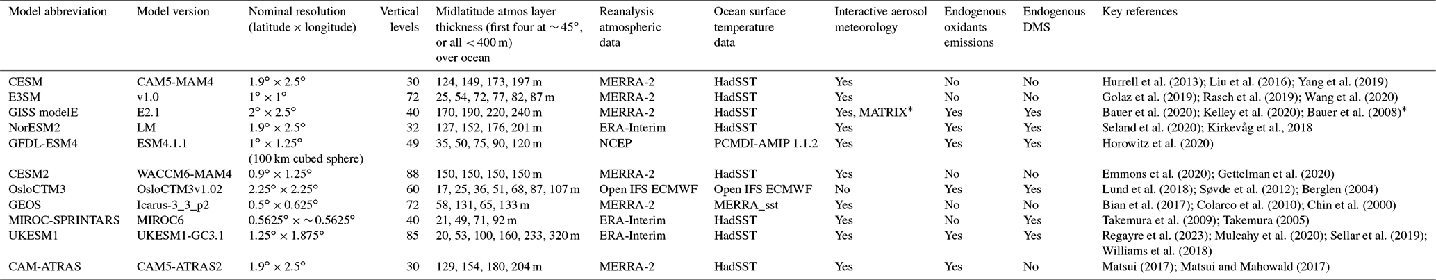
This study uses output from 11 climate–aerosol and chemical transport models (CTMs) participating in Emissions-MIP. The simulation setup uses atmosphere-only model runs with prescribed sea surface temperatures (SSTs) and sea ice concentrations, as well as nudged winds for atmospheric general circulation models (AGCMs) and prescribed meteorology for CTMs. A summary of model characteristics is provided in Table 1. Additional details on the aerosol module in each model is included in Supplement Table S1.
Table 1Models used in this study including relevant model characteristics.
2.2 Experiments
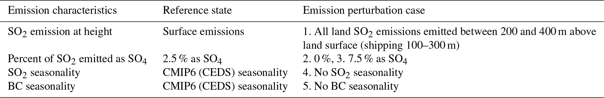
Each modeling group simulated the impact of five perturbations summarized in Table 2. These characteristics are either inconsistently represented in emission datasets (seasonality) or are inconsistently implemented in individual models (effective injection height, emitted SO4 fraction). Each experiment uses atmosphere-only model simulations running for a 5-year period from 2000 to 2004 following the year 1999 spin-up as needed by each model. Refer to the file Emissions-MIP Experimental Protocol – v1b.xlsx in the Supplement for a more detailed breakdown of the model settings for each experiment. The reference case that is used as the base experiment for comparison consists of the reference state conditions indicated in Table 2.
2.3 Overview of perturbation assumptions
This section is a review of the setup for the perturbations examined in the study and discusses the motivation for choosing the specific sensitivity parameters used in each experiment. The base emissions data for these experiments are anthropogenic emissions as produced by the Community Emissions Data System (CEDS) for CMIP6 (Hoesly et al., 2018). Anthropogenic emissions as defined here exclude emissions from open burning of grasslands, forests, and agricultural residues on fields.
2.3.1 SO2 emission at height
Accurate emission data are dependent on spatial resolution and the vertical distribution of the emissions (Pozzer et al., 2009). However, an underlying cause of uncertainty is the injection height of anthropogenic emissions in global models (Yang et al., 2019). Most studies that have examined the impact of the injection height of anthropogenic emissions used regional models (Akingunola et al., 2018; Mailler et al., 2013). Pozzer et al. (2009) examined the impact of applying a vertical distribution to anthropogenic emissions using a global atmospheric chemistry model. Although a strong height dependence was observed for NOx, CO, NMVOCs, and O3, the impact of vertical distribution on SO2 emissions was not considered in that study. This is a significant limitation since SO2 is sensitive to vertical distribution to a greater extent than other species (Bieser et al., 2011). Yang et al. (2019) showed that the assumed effective emission height (i.e., stack height combined with plume rise) had a large influence on SO2 near-surface concentrations and vertical profile in CAM5, a global aerosol–climate model. It was found that the range of near-surface SO2 concentration over land due to uncertainty in industrial emission injection height was 81 % relative to the average concentration. This result raises the question of whether the sensitivity to injection height is similar across models, and if so, to what extent.
Any factor that impacts SO2 surface concentrations will also have implications for evaluating models against observations (at the surface or column burdens retrieved by satellites). Since direct SO2 concentration measurements are mostly available at the surface, any attempt to validate the sulfur chemistry in the model will be impacted by the injection height assumptions (Johnson et al., 2020). Therefore, systematic assignment of emission data to vertical model layers is important (Pregger and Friedrich, 2009). Global climate and chemistry models generally rely on assumptions of the height dependency of anthropogenic emissions, such as from the AeroCom (Aerosol Comparisons between Observations and Models) simulation protocol (de Meij et al., 2006; Stier et al., 2005). According to the AeroCom protocol, emissions from industrial facilities and power plants should be injected evenly at a height of 100 to 300 m above the surface, and emissions from international shipping are injected into the lowest model layer (Dentener et al., 2006). No recommendation on assumptions for effective emission injection height was provided as part of CMIP6. However, the height of plume rise has been measured to exceed these assumed heights by up to 1 km, as was the case for SO2 emissions emitted by flare stacks in the Athabasca oil sands (Akingunola et al., 2018; Gordon et al., 2018). While this is only one example, it indicates that the effective injection height for anthropogenic sources can be quite large and that there is substantial variability due to changes in meteorology. Ship stacks may be underestimated with respect to their height, as the largest ships (e.g., Panamax) could have a maximum height of 60 m above sea level (Chosson et al., 2008). The plume rise may then extend the emission height by several hundred meters.
Therefore, for the sensitivity case used here we specify slightly higher effective injection heights (Table 2) compared to those used in the AeroCom study. For the Emissions-MIP emission height perturbation anthropogenic SO2 (and associated SO4) over land was specified to be distributed over 200–400 m above the land surface, and the shipping sector emissions were distributed over 100–300 m above the ocean surface. Emission amounts were assumed to be distributed evenly across the specified altitude range and proportionally allocated to the relevant model layers.
2.3.2 Emitted sulfate fraction
A number of studies have focused on sulfur chemistry within sulfur-rich plumes, as these are a large fraction of anthropogenic aerosols (Wei et al., 2022; Stevens and Pierce, 2013). Global- and regional-scale models are generally unable to accurately resolve aerosol formation within these plumes using grid cells that are tens of kilometers in size or more (Fast et al., 2022; Stevens and Pierce, 2013). It is typical for these models to assume that a fraction of anthropogenic SO2 emissions is emitted into the model grid as sulfate. For instance, the AeroCom protocol suggests that 2.5 % of sulfur should be emitted as sulfate, where most sulfur is emitted as SO2 (Dentener et al., 2006). Luo and Yu (2011) found that increasing the fraction of emitted SO2 converted to sub-grid sulfate from 0 % to 5 % yielded a change in global boundary layer CCN0.2 (i.e., CCN number concentration at 0.2 % supersaturation) by 11 %. Wang and Penner (2009) demonstrated that even a moderate increase in the SO2 fraction converted to sub-grid sulfate from 0 % to 2 % resulted in an increase in CCN0.2 by 23 % in the boundary layer. Both studies highlighted the importance of accurate parameterizations of sub-grid-scale sulfate formation in global aerosol models.
The work cited above focuses on strong emission sources from sulfur-rich plumes. However, these are becoming less commonplace as SO2 emission controls become more stringent. Current emission controls focus on removing solid particulates and gaseous SO2. Wu et al. (2020) find that 18 % of the sulfur emitted at the stack can be in the form of either filterable or condensable particulates. Further conversion to sulfate occurs in stack plumes (Ding et al., 2021; Luria et al., 2001), which has long been observed to be linear in many cases (Luria et al., 2001) but may be more rapid in wet plumes (Ding et al., 2021). Further, as noted later, a large portion of the emitted sulfur is in the form of SO3.
If we were to assume that 30 % of the sulfur from power plants in China is in the form of SO3, then one could have an aggregate SO3 fraction (for all sectors) over China of up to 8 %–9 % (in S mass units). This suggests that, at least in some instances, a much higher fraction of SO2 should be assumed to be emitted as sulfate in global models since SO3 is quickly converted to H2SO4 and sulfate in the presence of water vapor (see also the Conclusions section).
Anthropogenic emission inventories typically specify a total amount of sulfur emissions (as SO2). For the present study, we examined two sensitivity cases for SO2 to SO4 sub-grid conversion, i.e., a “no SO4” case and a “high SO4” case, which are specified to have 0 % and 7.5 % (as %S) anthropogenic SO2 emitted as sulfate, respectively. Emissions of SO2 are reduced proportionately so as to preserve the total emitted mass of sulfur.
2.3.3 Seasonality
Another source of uncertainty in emission data is the temporal distribution, namely seasonality (i.e., monthly patterns). We note that diurnal and weekly patterns can also influence results; however, these are not evaluated in this work. Aerosol formation and transport (Stohl et al., 2013), as well as chemical reaction rate (Sofiev et al., 2013; Pregger and Friedrich, 2009), are dependent on the season. Therefore, aerosol and precursor species can have a longer or shorter lifetime depending on the emission seasonality in the model. The emissions data used for CMIP6 (Hoesly et al., 2018) incorporated estimates of seasonality for all sectors and emissions, while the data for prior CMIP phases had partial or no seasonality information. It will be useful to evaluate this aspect of the data to inform our understanding of the role of aerosols in earlier CMIP experiments.
Aside from openly occurring forest or grass fires which are typically a large source of BC emissions during the summer, combustion of biomass such as residential wood for heating homes during the winter is a significant source of BC seasonality (Healy et al., 2017). The other major driver of seasonality in aerosol or precursor emissions is space cooling (e.g., air-conditioning), which results in some seasonality in electric power production (Sofiev et al., 2017). There is significant seasonality in emissions associated with biological processes, in particular ammonia (Wang et al., 2021), although we did not evaluate this here because that requires models that have sufficiently detailed chemistry.
The two sensitivity scenarios that were considered were identical monthly (averaged annually) emission fluxes for all anthropogenic SO2 emissions (including associated SO4) and anthropogenic BC emissions as compared to the seasonality used in CMIP6, which is used in the reference case (Table 2).
2.4 Data processing
Much of the basic data processing in this study was performed with the Earth System Model Evaluation Tool, ESMValTool v2.1.1 (Andela et al., 2020), an open-source diagnostic tool available for the evaluation of Earth system models (Eyring et al., 2020). Simulation results were made available by the participating model groups as netCDF files and, where necessary, processed to conform to the CMIP format (i.e., the data have been “CMORized”) for use with ESMValTool. Minor issues in the netCDF files (e.g., missing metadata) were corrected using tools such as netCDF Operator (NCO) or Climate Data Operator (CDO). The datasets from the E3SM, CESM, and CESM2 models were CMORized using e3sm_to_cmip, an open-source tool that converts E3SM (and CESM) model output variables to the CMIP format (Baldwin et al., 2021).
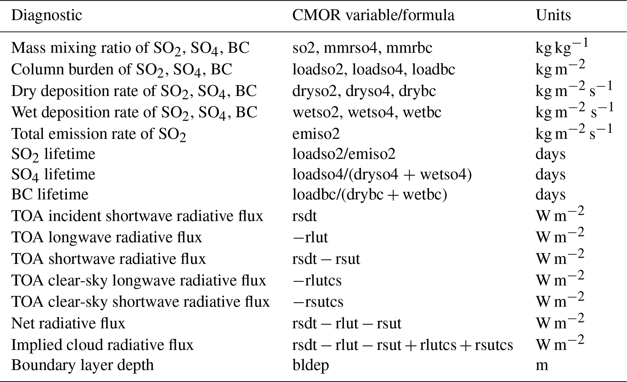
The ESMValTool workflow is controlled by a “recipe” file that defines the datasets, preprocessor options, and diagnostics. All model results were interpolated to 1∘ × 1∘ grids and the annual mean taken either over the globe or masked to a specific region or ocean basin (Fig. S1 in the Supplement). This functionality was used to compare the impact of emission characteristics in different regions. Each model simulation provided variables for gas and aerosol concentrations and deposition rates as well as radiative fluxes at the surface and top of the atmosphere. Table 3 provides a list of the variables used in the analysis.
Table 3Diagnostics extracted or calculated from model simulations. TOA: top-of-atmosphere.
In this section we assess the extent to which the perturbation results differ from the reference scenario as well as the spread of response in models for each experiment. Section 3.1 focuses on the lifetime diagnostics, namely sulfur and BC lifetimes. Section 3.2 provides an overview of the radiative flux results. Section 3.3, 3.4, and 3.5 offer a more detailed look at the SO2 emission at height, emitted sulfate fraction, and seasonality simulation results, respectively.
3.1 Sulfur and BC lifetimes
Among the central factors that influence model emissions responses are the atmospheric lifetimes of BC, SO2, and sulfate. In this section we examine how reference case lifetimes vary between models as context for the analysis of perturbation responses in the next sections. Figure 1 shows the sulfate lifetime averaged over the globe and an approximate SO2 lifetime (i.e., SO2 column burden divided by emission rate of anthropogenic SO2) averaged over the Northern Hemisphere (NH) land area. Sulfate lifetime was calculated as sulfate column burden divided by the sum of the dry and wet sulfate deposition rates. SO2 lifetime was calculated as SO2 column burden divided by the emission rate of anthropogenic SO2. The source term (i.e., anthropogenic SO2 emission flux) was used for SO2 lifetime since not all sink terms for SO2 (i.e., gas-phase and aqueous-phase oxidation; Liu et al., 2012) were available from the standard output of the models. Although the SO2 lifetime as calculated here will be biased high since dimethyl sulfide (DMS) and volcanic source terms were not used in the calculation (diagnostic data were not available for all models), we focus on the value over NH land where anthropogenic emissions dominate and this source of bias is small compared to the inter-model variation.
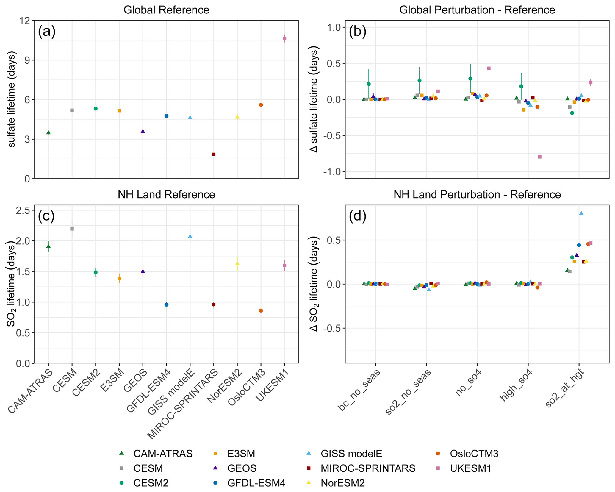
Figure 1(a) Global sulfate lifetime (c) and Northern Hemisphere land SO2 lifetime for the reference case model simulations, as well as the (b, d) absolute difference between each perturbation and the reference case. Refer to Fig. S2 for the Northern Hemisphere land sulfate lifetime. All results are averaged over the years 2000–2004, except NorESM2, which is averaged over 2001–2005. The bars represent interannual variability (±1σ). Note that the large uncertainty bars for CESM2 sulfate lifetime are due to the high interannual variability in the sulfate column burden.
The sulfate lifetime for the reference case in Fig. 1a is 5 d on average, with a range of 3.5–5.6 d excluding two outlier values. The lifetime for UKESM1 was considerably higher at 10.6 d due to the low wet deposition rate of sulfate in this version of the model. UKESM1 emits primary SO4 at a relatively small diameter of 100 nm (geometrical mean), which reduces cloud droplet nucleation efficiency. The version of the model used in the current study also has a relatively high scavenging diameter (i.e., the particle diameter above which particles are removed in large-scale rain events, prescribed here as 150 nm), which increases the number of particles that pass through clouds to reach higher altitudes and thus increases sulfate lifetime. The other outlier value was MIROC-SPRINTARS, with a sulfate lifetime of 1.8 d. In part, this low value is because this model is known to exhibit a lower sulfate lifetime in nudged simulations using reanalysis atmospheric data in which the response of precipitation tends to be excessive. It is not known if this effect exists in other models. In simulations without constraining meteorological fields, the sulfate lifetime is approximately doubled, which would be closer to the central range.
Models showed a greater relative variation compared to that for SO4 for the mean SO2 lifetime of 1.5 d over NH land, as depicted in Fig. 1c, with a range of 0.9 to 2.2 d. The variation in the SO2 lifetime response is nearly proportional to that of SO2 column burden (numerator) since the anthropogenic SO2 emission rate (denominator) is very similar across models (Fig. S3). SO2 lifetime was also examined over the globe (Fig. S4) to compare the relative impact of DMS chemistry, which could be a potential source of variation. The global mean SO2 lifetime was 1.8 d and ranged from 1.3 to 2.5 d. When averaged across all models, the global SO2 lifetime is 20 % greater than for NH land. The SO2 column burden is 2.4 times higher over NH land but the emissions rate of anthropogenic SO2 is 3 times higher compared to the global mean. Dry and wet SO2 deposition (Fig. S5) constitutes about 70 % of the total sink in NH land on average and does not have a strong correlation with SO2 lifetime (i.e., poor linear relationship).
Figure 2 shows the global BC lifetime, which is the BC column burden divided by the sum of the dry and wet BC deposition (wet deposition is the dominant factor at about 3 times as high on average – Fig. S6). In Fig. 2a, the global BC lifetime is 5.6 d, with a fairly large range of 3.7–8 d. This global average and range are consistent with results from recent studies (Gliß et al., 2021; Lund et al., 2018; Kristiansen et al., 2016; Samset et al., 2014). Removing BC seasonality had an impact on global BC lifetime in some models as shown in Fig. 2b, with both positive and negative responses. GISS modelE and UKESM1 both exhibited a noticeable drop in BC lifetime of 0.48 and 0.29 d, respectively. The remaining models showed only a small increase in lifetime, with a maximum increase of 0.12 d for CESM2.
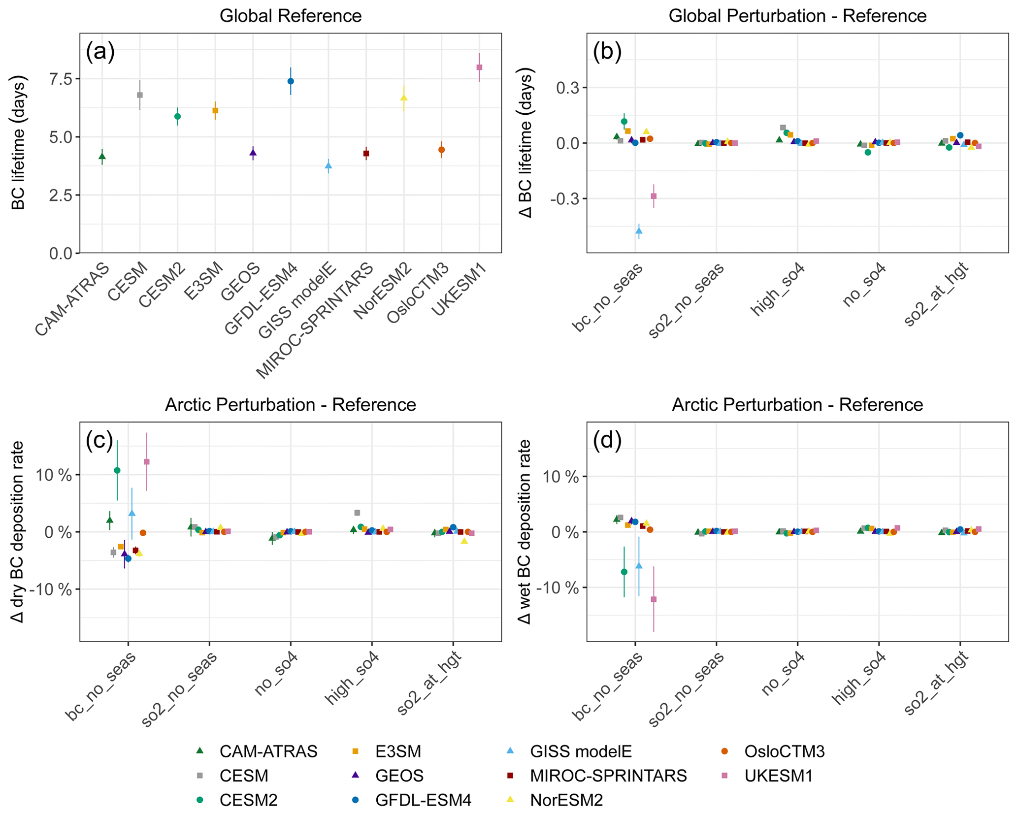
Figure 2(a) Reference case of global BC lifetime, (b) absolute difference of global BC lifetime for each perturbation, (c) percent difference of Arctic dry BC deposition rate, and (d) percent difference of Arctic wet BC deposition rate. All results are averaged over the years 2000–2004, except NorESM2, which is averaged over 2001–2005. The uncertainty bars represent interannual variability (±1σ).
3.2 Radiative flux
Figure 3 shows the impact of the perturbations on the radiative flux at the top of the atmosphere (perturbation experiment minus the reference case), where a positive change denotes an increase in the Earth's energy imbalance (a generalized heating effect), and a negative change denotes a decrease in the Earth's energy imbalance (a generalized cooling effect).1 Clear-sky longwave flux showed a minimal response, which is consistent with fixed SST experiments (since longwave flux would be driven largely by surface temperature changes, which are limited in fixed SST experiments). SO2 emission at height consistently decreased clear-sky shortwave flux, leading to increased cooling, with a few models showing a fairly large response (e.g., GISS modelE at −0.5 W m−2 and OsloCTM3 and UKESM1 at around −0.3 W m−2). The implied cloud response exhibited a diversity of magnitude and sign. NorESM2 had the largest change resulting from the emission height experiment, with a decrease in cloud forcing by −0.19 W m−2. OsloCTM3 and GISS modelE exhibited the largest increase in cloud forcing by 0.15 and 0.11 W m−2, respectively. However, OsloCTM3 only includes the direct aerosol effect, and thus changes in the cloud forcing are associated with cloud response to atmospheric adjustment rather than aerosol–cloud interactions. All remaining models showed a moderate decrease in the cloud response. Further details on radiative flux are discussed in the following sections as they pertain to the specific perturbation experiments.
These changes are potentially large compared to the effective radiative forcing (ERF), which is the sum of aerosol–radiation interactions (ARIs) and aerosol–cloud interactions (ACIs), as reported in the Intergovernmental Panel on Climate Change (IPCC) Sixth Assessment Report – AR6 (Forster et al., 2021). The best estimate of ERF (2019 relative to 1750) in AR6 is −1.06 W m−2 (i.e., ERF = ARI + ACI, where ARI and ACI are −0.22 and −0.84 W m−2, respectively; Szopa et al., 2021). The changes in global mean net radiative flux we found here, for at least some models, make up a significant fraction of these values. Note that in this study we are looking at differences in radiative flux and did not formally calculate ERF, so this is only an approximate comparison.
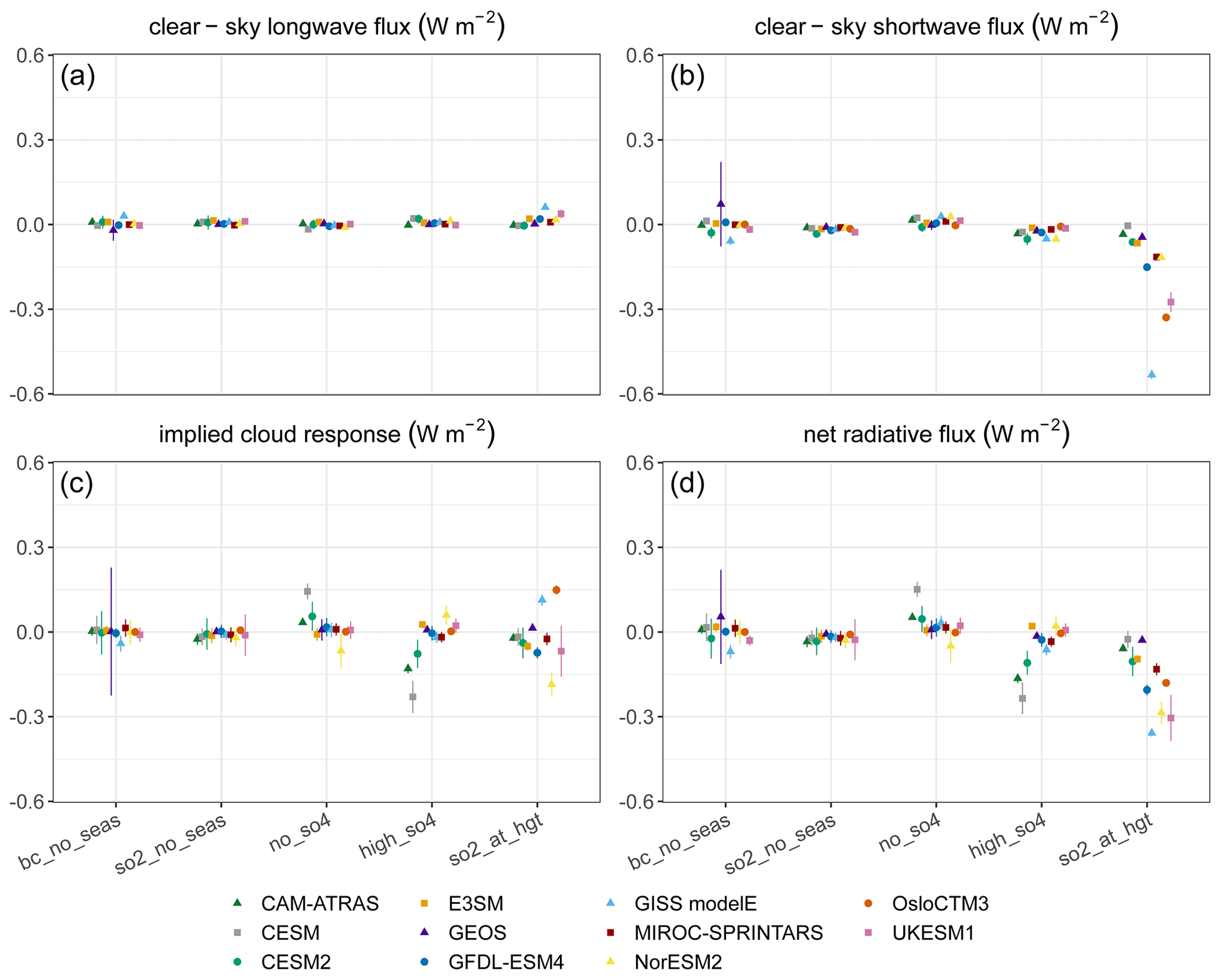
Figure 3Absolute difference (perturbation – reference) of global mean (a) clear-sky longwave radiative flux, (b) clear-sky shortwave radiative flux, (c) implied cloud response (which is the net forcing minus the sum of clear-sky longwave and shortwave flux), and (d) net radiative flux averaged over the years 2000–2004 (NorESM2 averaged over 2001–2005). Interannual variability (±1σ) is shown as thin lines. Note that GEOS was averaged over 2001–2004 (the year 2000 was omitted to reduce interannual variability presumably introduced by having a 3-month spin-up, which may be short for radiation fields) for the radiative flux variables (Table 3), and changes for OsloCTM3 are only due to aerosol–radiation interaction.
3.3 SO2 emission at height
The SO2 emission at height results exhibited both increases and decreases in sulfate lifetime (Fig. 1b). CESM and CESM2 showed a decrease and UKESM1 had an increase in lifetime. The reason for this is nuanced since emission at height not only increased sulfate dry and wet deposition, but it also increased the sulfate column burden. The signs of these two effects were consistent across all models. Therefore, an increase in both the numerator and denominator may result in either a positive or negative difference (i.e., perturbation experiment minus reference) depending on the relative magnitude of each effect. Overall, the emission height assumption had a relatively small impact on sulfate lifetime for most models.
Turning to SO2 lifetimes, Fig. 1d shows that emission at height consistently increases SO2 lifetime over Northern Hemisphere land. The largest increase is 0.8 d in GISS modelE, with an average of 0.31 d across the rest of the models (range of 0.14–0.47) and a proportionate increase in SO2 column burden (Fig. S7). We also note that the four highest model responses (GISS modelE, UKESM1, OsloCTM3, GFDL-ESM4) all have endogenous oxidants in their model configuration. The total SO2 deposition rate dropped across all models (Fig. S8), with an average increase in wet SO2 deposition rate of 1.5×10⁹ kg yr−1 (21 %), which is smaller than the average drop in dry SO2 deposition rate of 1.2×10¹⁰ kg yr−1 (40 %). Emission at height, therefore, also results in a shift from dry to wet deposition.
As the sink via deposition becomes slower (due to being further emitted from the surface), the other sink pathway (conversion to SO4) becomes more important. While we do not have diagnostics available for chemical conversion, we can infer the relative importance of deposition vs. chemical conversion by estimating the change in atmospheric lifetime if we assume a constant atmospheric SO2 oxidation rate. We find that the change in SO2 lifetime is smaller by an average of a factor of 1.7 (range 1.3–2.0) than seen in the model results (Fig. S9 and Table S2) if the only change is SO2 deposition. This means that the SO2 lifetime increase due to decreased deposition for emission at height is being significantly offset by an increase in the rate of SO2 conversion to SO4 through either gas-phase or aqueous-phase processes. This is also indicated in the change in sulfate burden change, which exhibits a reasonable correlation with the offset in SO2 lifetime (Fig. S10). In summary, we find that as SO2 is emitted at height, dry SO2 deposition decreases as the overall lifetime of SO2 in the atmosphere increases (Fig. 1d). The longer atmospheric residence time, in turn, increases chemical conversion of SO2 to SO4, which subsequently causes an increase in SO4 in the atmosphere (Fig. 6b).
For SO2 emission at height, there were small positive and negative changes in BC lifetime. The reason for these changes may be due to aerosol mixing between BC and sulfate or atmospheric adjustments.
Of the perturbations considered, the experiment with emission at height had the largest impact on net flux, with impacts of up to −0.35 W m−2 for GISS modelE, two additional models at around −0.3 W m−2, and the remaining models ranging down to nearly zero (Fig. 3d). Figure 4 shows a global map of the net radiative flux for the models showing the largest impact. The range in net forcing is a combination of the range in individual forcing responses and the fact that the cloud responses have different signs. This has important implications for model calibration and tuning. For instance, OsloCTM3 and GFDL-ESM4 exhibited a similar net flux response, but the radiative flux components that contribute to the net flux differed significantly. With GFDL-ESM4, a modest change in the cloud response and clear-sky shortwave flux combined into a large change in net flux. However, for OsloCTM3 these terms were both large but of opposite sign. This diversity of responses is an indicator of the significant uncertainty in the underlying mechanisms driving aerosol forcing across models.
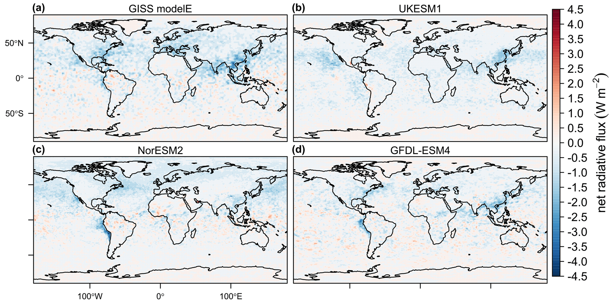
Figure 4Global maps of models with the highest absolute differences (i.e., emission at height – reference) in global mean net radiative flux, averaged over the years 2000–2004 (NorESM2 averaged over 2001–2005) – (a) GISS modelE, (b) UKESM1, (c) NorESM2, and (d) GFDL-ESM4.
Examining the SO2 emission height results in more detail, we find a strong relationship between the change in clear-sky shortwave forcing and change in sulfate column burden (Fig. 5a). The change in sulfate column burden ranges from 0 % to 25 % (Fig. S11) relative to the reference case. With a couple of outliers, this relationship is remarkably linear across the models given the many factors that could potentially influence this relationship such as sulfate particle size distribution, optical properties, and mixing treatment, although we note that a number of models represented here have aerosol schemes related to the CESM family of models (Liu et al., 2012, 2016). GISS modelE, given the column burden change, has a stronger relative shortwave response compared to the other models, potentially due to new particle formation (i.e., the formation of Aitken-sized sulfate particles from binary nucleation) and the interaction with nitrate aerosol formation processes, as well as a stronger height dependence for sulfate production. The sulfate column burden is driven by an increase in SO2 column burden, since emitting SO2 at height (Fig. S12) consistently increases SO2 lifetime (Fig. 1d). Although the sulfate lifetime did not show a consistent change due to the emission at height experiment (Fig. 1b), there was an increase in sulfate in the atmosphere (Fig. S13) due to the increase in SO2 column burden, as illustrated in Fig. 5b. This is a fairly linear relationship, with the exception of the OsloCTM3 model, which showed a stronger response to SO2 column burden. The reasons for this different response were not clear but are perhaps due to nonlinearity in lifetime changes with height.
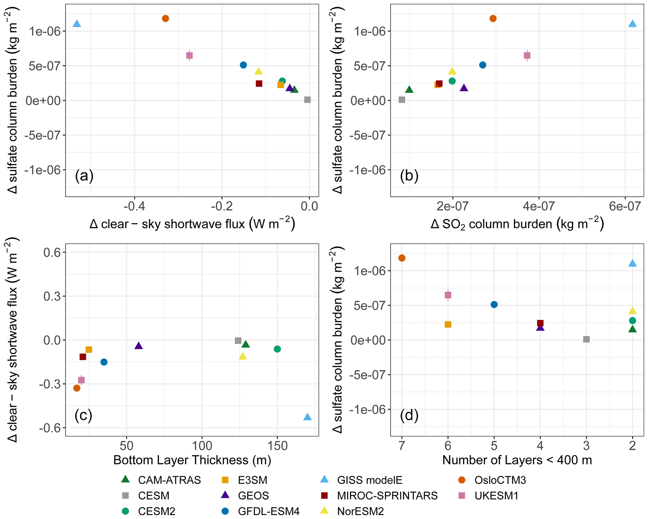
Figure 5Impact of SO2 emissions at height on the relationship between (a) sulfate column burden vs. clear-sky shortwave flux changes, (b) sulfate column burden vs. SO2 column burden changes, (c) clear-sky shortwave flux change vs. bottom model layer thickness, and (d) sulfate column burden change vs. number of model layers below 400 m.
Model vertical resolution was another factor that has an impact on these results, particularly for the SO2 emission height experiment. Figure 5c shows that with increasing model vertical resolution (i.e., decreasing layer thickness) the model response increased, except for GISS modelE. The relatively coarse vertical model resolution in GISS modelE introduces stronger sensitivities to the collocation of aerosol and cloud layers and therefore strongly impacts aerosol–cloud interactions, such as in-cloud aqueous chemistry rates, aerosol activation, and wet removal. We observe a cluster of relatively high- and low-resolution models. The high-resolution models have a stronger clear-sky shortwave flux response in general, but still with variation across this subset of models. Two of the models with a relatively high response (i.e., OsloCTM3 and UKESM1) are higher-resolution models. In contrast, E3SM had a lower sensitivity compared to the other high-resolution models, as also shown by Fig. 5d, which illustrates a fairly linear relationship between sulfate column burden change for models with more than two layers below 400 m, excluding E3SM. Although E3SM has the same number of layers below 400 m as UKESM1, it had a notably smaller sulfate burden response, likely due to a difference in the treatment of sub-grid vertical mixing and transport. Differences in SO2 lifetime do not appear to explain the shortwave response among the high-resolution models (Fig. S14) since the difference in OsloCTM3 and UKESM1 lifetime is relatively large (0.75 d).
The SO2 emission height experiment also had a substantial impact on the surface concentrations of SO2, with some of the highest relative changes for any variable examined (Fig. 6a). Globally averaged SO2 surface concentrations dropped with emission at height by an average of 39 % relative to the reference case with a range of 9 %–59 %. In terms of regional responses, the SO2 surface concentration dropped more significantly over land (46 % on average) compared to over the oceans (6 % on average), as shown in Fig. S15.
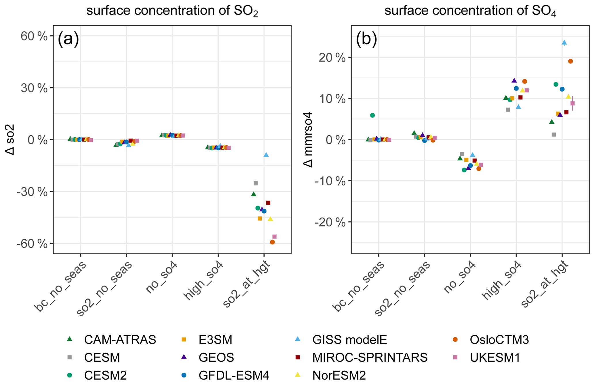
Figure 6Global percent difference (perturbation – reference) reference in the (a) surface concentration of SO2 and (b) surface concentration of SO4. All results are averaged over the years 2000–2004, except NorESM2, which is averaged over 2001–2005. The bars represent interannual variability (±1σ).
The SO2 emission height had the opposite effect on the surface concentration of SO4, with an average increase of 10 % in global surface SO4 concentration ranging from 1 % to 23 % (Fig. 6b). The average model surface sulfate concentration increased by a similar amount over land (10 %) and over oceans (11 %), as shown in Fig. S16. Given that there is little change in sulfate lifetime (Fig. 1b), the increased surface sulfate appears to be the result of increased conversion of SO2 to sulfate due to decreased dry deposition of SO2.
A strong relationship between column burden change and surface concentration change of SO4 is observed in the emission height experiment (Fig. S17). There is not, however, a consistent relationship across models between changes in SO2 column and surface concentrations. This is due in large part to the shorter SO2 lifetime (Fig. 1c) that results in more variation in the relationship between SO2 surface and column changes. Also, since SO2 is injected directly into the bottom model layer as opposed to a higher layer, we would expect a larger change in surface concentrations given the same column burden. This is evident in Fig. S18, where the higher-resolution models (i.e., models with smaller bottom layer thickness) are shown to have a larger drop in SO2 surface concentration in the emission height experiment.
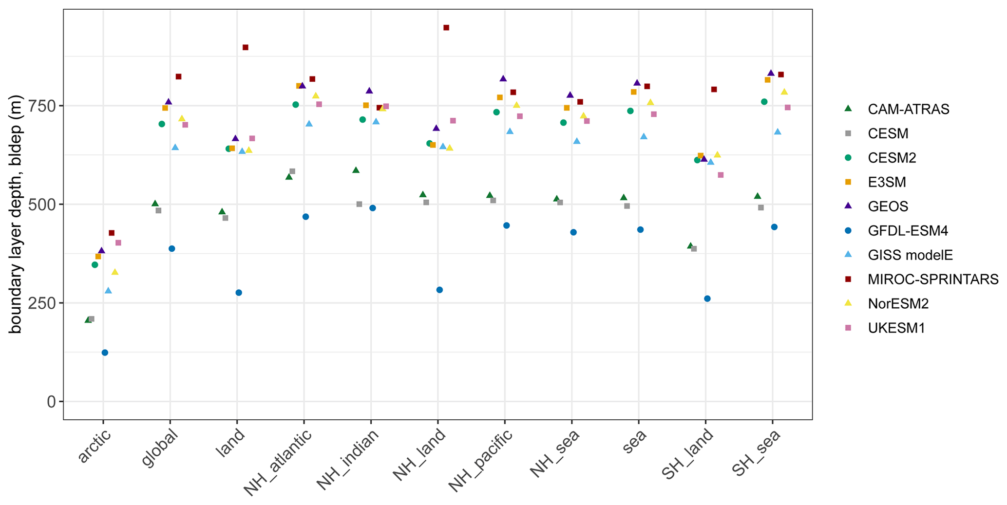
The emission height protocol described in Sect. 2.3.1, which distributed emissions to 200–400 m above land surface, falls below the average model planetary boundary layer height (PBLH) of 637 m over NH land as shown in Fig. 7. The average PBLH over NH land has four models clustered together at around 650 m, although the full range across models is 283–947 m. While the emission height is lower than the average PBLH, it is important to consider that the PBLH can be considerably lower during the night, for example around 250 m during the night compared to 800 m during the day (Svensson et al., 2011). Since there is more stratification of the PBLH during night, emission height can make a bigger difference, but it is not clear how the PBLH interacts with mixing schemes in the models and how they behave diurnally (Maier et al., 2022). In the context of the current study, this suggests that some of the emissions would be above the boundary layer during the night, which may explain why emission height has a significant impact on some model results. While there was no apparent correlation between average PBLH and the emission height results, we did not have diurnal PBLH information from the models.
3.4 Emitted sulfate fraction
When the sulfate fraction of emissions is increased sulfate lifetime decreases (and conversely with no S emitted as SO4), although the effect is small for some models (Fig. 1b). This result is explained by changes in sulfate deposition, which increases with a higher emitted sulfate fraction, while the sulfate column burden showed minimal changes. Note that this is in the baseline experimental setup with all emissions injected to the lowest model layer, where more SO2 emitted as SO4 can be more readily lost to dry deposition, although the strength of this effect varies by model. This may be dependent on the depth of the lowest model layer (i.e., change in sulfate deposition due to a higher sulfate fraction generally increases with layer thickness, as shown in Fig. S19).
The sulfate emission fraction also consistently changed the BC lifetime in a couple of models. CESM2 showed a slight increase (less than 0.1 d) in BC lifetime in the no sulfate fraction experiment and a decrease in lifetime by a similar magnitude in the high sulfate fraction experiment. CESM and E3SM also showed an increase in BC lifetime for no sulfate but a smaller decrease in lifetime for a high sulfate fraction.
Increasing the sulfate emission fraction consistently decreased clear-sky shortwave flux slightly, but the largest changes were to cloud response (Fig. 3c), again with both positive and negative responses in different models. The responses to sulfate fraction perturbations may be a reflection of the cloud cover change (Fig. S20), which is generally positive (i.e., an increase in cloud cover) for high sulfate fraction and negative for no sulfate upon emission. However, the NorESM2 cloud response had the opposite sign compared to the other models for the sulfate fraction experiments. This appears to be due to a response in ice water path (Fig. S21), which shows a relatively strong response for NorESM2, with an increase for the high sulfate experiment and decrease for the no sulfate experiment.
The high sulfate fraction experiment yielded a decrease in the net radiative flux and cloud response, averaging −0.064 and −0.036 W m−2 across the models, respectively. This is consistent with the notion that sulfate aerosols can act as CCN and affect cloud formation, as well as having a cooling effect on the climate (Takemura, 2020). The experiment with no sulfate emission fraction exhibited opposite signs in net radiative flux and cloud response for most models, with an average of 0.018 and 0.015 W m−2 across models, respectively. This experiment also shows a decrease in cloud cover for nearly all models (Fig. S20).
Furthermore, the assumption about the primary sulfate emission fraction had an impact on the global surface SO4 concentration. As illustrated in Fig. 6b, the high sulfate fraction experiment yielded an average increase in surface concentration of about 11 %, and the no sulfate emission experiment resulted in a drop of about 6 %.
3.5 Seasonality
The no SO2 seasonality experiment showed a consistent increase in sulfate lifetime of 0.06 d averaged over all models. The underlying cause of this change can be attributed to the difference in sulfur emissions between the Northern and Southern Hemisphere. The Northern Hemisphere generally experiences more seasonal emissions changes due to energy consumption for heating in the winter months. The increase in the total sulfate deposition rate in the Northern and Southern Hemisphere with no emission seasonality, averaged across all models, is and kg m−2 s−1, respectively (Fig. S22). This is further corroborated in Fig. 8, which shows a higher sulfate lifetime in the Northern Hemisphere due to SO2 seasonality with the exception of CESM2, which is inconclusive.
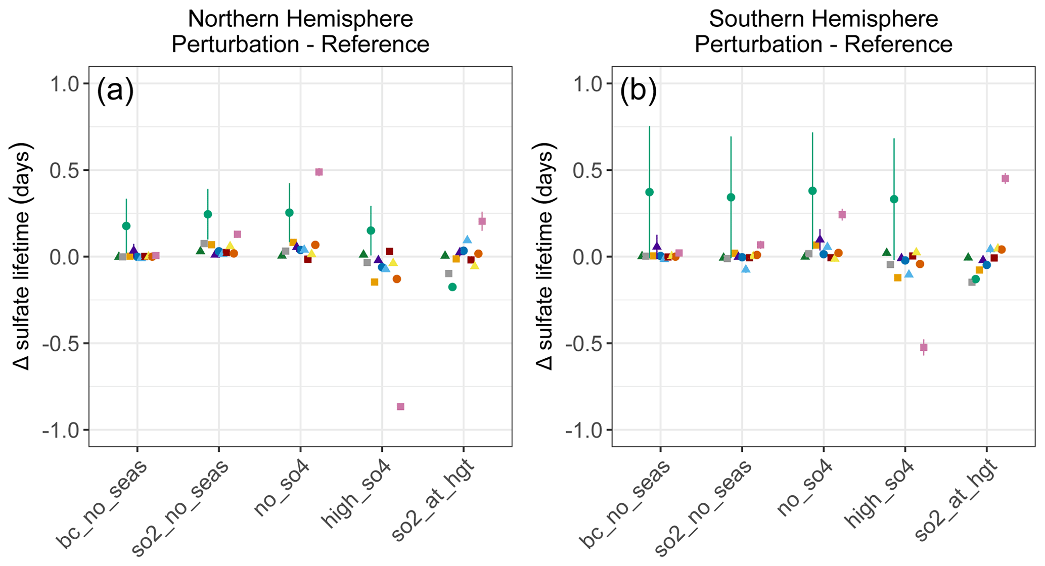
Figure 8Absolute change in sulfate lifetime averaged over the (a) Northern Hemisphere and the (b) Southern Hemisphere. The bars represent interannual variability (±1σ).
Previous studies have shown that the Arctic BC concentration, deposition, and source attributions have a strong seasonality (Matsui et al., 2022; Ren et al., 2020; Wang et al., 2014, 2013; Stohl et al., 2013). We also find that BC deposition rates in the Arctic are sensitive to BC seasonality, although not consistently across models. In the reference case, based on CMIP6 historical data, BC emissions in the Arctic were at a maximum of 2.9 kt in January and a minimum of 1.9 kt from June to August, as shown in Fig. 9a. The global BC emissions in Fig. 9b also show a maximum and minimum during winter and summer, respectively, although the degree of seasonal variation is not as distinct. The impact of seasonality on deposition is not consistent between models, with one set of models showing an increase in dry deposition when emission seasonality was removed, while another set shows the opposite behavior, although at a lower magnitude (Fig. 2c). The opposite behavior is seen for wet deposition except for CAM-ATRAS (Fig. 2d). In the CAM-ATRAS model, seasonality increases BC transport to the Arctic during the winter, which may increase the annual mean BC concentration as well as dry and wet deposition in the Arctic. The simulated seasonal variability of precipitation is a potential driver of the differences observed between models, as are BC transport and height. We note that the interannual variability for models with an increase in dry BC deposition was much more prominent than for models that showed a decrease.
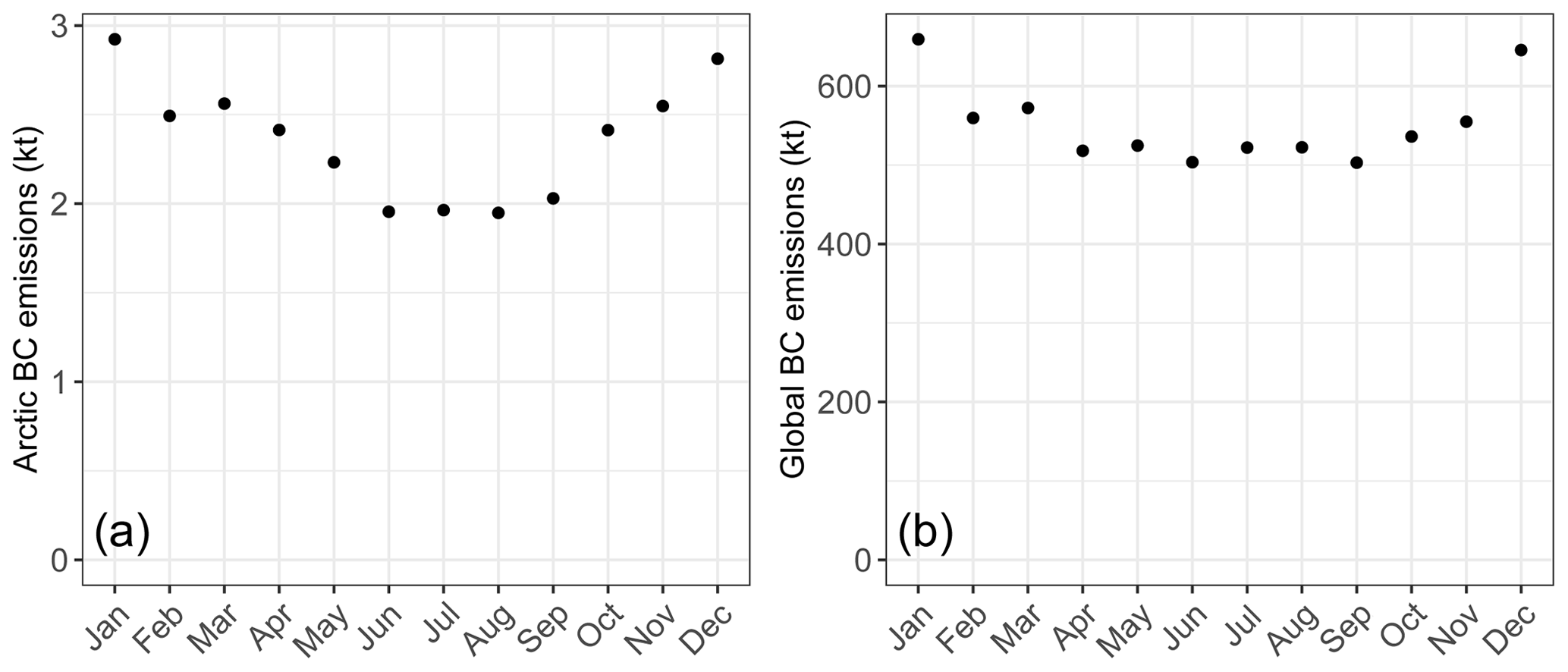
Figure 9Reference case (a) Arctic BC emissions (> 66∘ N) and (b) global BC emissions based on monthly CMIP6 data for 2004.
SO2 seasonality did not have a large impact on any of the forcing metrics. BC seasonality had a slightly larger impact, particularly for GISS modelE, but the magnitude of the effect was small (Fig. 3).
This study explored the sensitivity of 11 climate–aerosol and chemical transport models to four emission characteristics: SO2 emission height, SO2 seasonality, BC seasonality, and the fraction of SO2 assumed to be SO4 upon emission. Each perturbation experiment used atmosphere-only model simulations with specified sea surface temperatures and nudged winds, running for a 5-year period following 1 year of spin-up. Of the perturbations examined in this study, the assumed height of SO2 injection had the largest overall impacts, particularly on net radiative flux (maximum absolute difference of −0.35 W m−2), but also on SO2 lifetime over NH land (maximum absolute difference of 0.8 d), surface SO2 concentration (up to 59 % drop), and surface sulfate concentration (up to 23 % increase). The sulfate emission fraction had a nontrivial impact in some models, particularly for net radiative forcing and surface SO4 concentration. SO2 and BC seasonality did not have a substantial impact on the global annual mean simulation results. However, BC seasonality had a slightly larger impact on net radiative forcing and had a significant effect on BC deposition in the Arctic, where we observed both positive and negative changes for both dry and wet deposition.
In general, the assumptions on emission height and SO4 fraction are a “hidden” source of inter-model variability because models have made different assumptions about these parameters. This is in addition to differences in model structure such as aerosol microphysical parameterizations. As demonstrated here, this unquantified source of differences may have a large impact on model results. Therefore, potential modifications or new datasets are needed for these parameters to both improve model results and remove a source of inter-model difference. Five of the models used here assume that all anthropogenic emissions are injected into the lowest model layer in their default setup. This will result in a bias in model results compared to reality for the bulk of SO2 emissions. Three of the models inject emissions either at 100 m or a higher level (100–300 m) for industrial and power generation sectors, which will still be an underestimate of injection height for some large sources (Akingunola et al., 2018). There was more uniformity in the fraction in SO4 fraction, with most models assuming that 2.5 % of SO2 is emitted as sulfate.
Assumptions on emission height, and to a lesser extent SO4 fraction, can have a very large impact on surface concentration values in the models. Evaluating model results by comparing with surface observations, particularly for SO2, will also be impacted by these assumptions. When evaluating models against observations the sensitivities explored in this work can be a potential source of bias. These issues also apply to satellite-based estimates, which generally incorporate assumptions about vertical distributions. For example, the Ozone Monitoring Instrument (OMI) aboard NASA's Aura satellite detects SO2 signals from anthropogenic sources (Fioletov et al., 2011) and has been compared with simulations by global models (Qu et al., 2019). These issues will be particularly large for satellite data products with more limited sensitivity to concentrations near the surface.
We find a large variation in atmospheric lifetime across models for SO2, SO4, and BC (particularly for SO2). The underlying drivers of this variation also likely drive some of the variation in results seen in the perturbation experiments. Better observational constraints on processes that influence aerosol lifetime (e.g., deposition, aerosol microphysical processes such as nucleation, coagulation, gas-to-particle conversion, aging – for BC) are needed to improve model physics and chemistry. Samset et al. (2014) used aircraft-based measurements of BC concentration to constrain BC radiative forcing and atmospheric lifetime in global aerosol–climate models, and this led to a reduction of 25 % in anthropogenic BC direct radiative forcing in remote areas relative to default model values. The UKESM1 model has recently incorporated updates to the aerosol removal processes, specifically through convective plume scavenging, nucleation scavenging, and dry deposition and sedimentation (Mulcahy et al., 2020). As part of a study to reduce uncertainty in the UKESM1 model through observational constraints, Regayre et al. (2023) show that dry deposition is one of the largest causes of uncertainty in aerosol forcing that remains largely unconstrained, even when other causes of uncertainty are tightly constrained. Better constraining SO2 chemistry in atmospheric models remains an important research goal for the community.
Model vertical resolution was found to have a large impact on the SO2 emission height experiment, with a higher vertical resolution corresponding to a stronger clear-sky shortwave flux response. However, there was still relatively large diversity in response among the high-resolution models. E3SM demonstrated a weaker sensitivity to clear-sky shortwave flux and sulfate column burden compared to the other high-resolution models (i.e., OsloCTM3 and UKESM1), so there are other underlying factors at work. We note that one of the last simulations done by most of the participating modeling groups was the emission at height simulation, as this required, in some cases, altering either model setup, data preprocessing, or internal model code. This points to the importance of carefully considering the best approach to incorporating these effects into global models. This also implies that emission inventories should contain data on emissions at different altitudes typical for the source categories (e.g., industry, transportation, shipping).
These results imply a need to ensure that anthropogenic emission injection height is accurately and consistently represented in global models. This is in addition to considering the impact of biomass burning injection height, which already has significant research (Veira et al., 2015; Paugam et al., 2016; Zhu et al., 2018). Collecting consistent data on emission stack height is one challenge, although such data often exist regionally (e.g., in the USA, Europe). In the context of models, we need the effective injection height, which is stack height plus plume rise, where plume rise is dependent on both stack characteristics, particularly effluent temperature, and meteorological conditions (wind speed, temperature, and the presence of any inversion layers). The effective injection height will also depend on the diurnal cycle of meteorology, PBLH, and stability. This points to the difficulty of providing accurate information on effective injection height globally. One option might be to implement plume rise parameterizations in global models. Another option is to collect information on the average amount of plume rise estimated in regional models to inform guidance for global models. Note that as model vertical resolution increases, the effects we found here become more important, and some solutions (such as plume rise parameterizations) may become more practical, or perhaps even necessary, for some model applications. At minimum models should clearly report their emission injection height assumptions, and model intercomparison exercises should consider whether standardized guidance should be provided.
The emissions at height perturbation experiment, in particular, is a novel diagnostic of the systemic response of a model to a fundamental change in emission characteristics. As discussed in the main text, the variety of model responses seen from this experiment reveals substantial variation and therefore uncertainty in aerosol dynamics and forcing responses across models.
We note further that the models used in these studies ignore SO3 emissions emitted at stacks, which may impact results. This is important since SO3 in the atmosphere can potentially form sulfuric acid, which in turn can nucleate or condense to existing particles. Coal plants in China with pollution controls in place have been found to emit up to 40 % of their sulfur in the form of SO3 (Wu et al., 2020). Other work seems to support the notion that the ratio of SO3 to SO2 increases as controls strengthen. Mylläri et al. (2016) established that flue gas cleaning technologies greatly reduce SO2 concentration, and they further suggest that SO3 may exist in the plume and can increase the probability of aerosol formation.
Current global inventory data are not necessarily consistent in accounting for emissions of different sulfur species (e.g., SO3 and SO2 gas, as well as filterable and condensable SO4 particles). Bottom-up mass balance approaches, which rely on data on fuel sulfur content, are implicitly reporting all sulfur-containing species as SO2. Inventories that rely on measurement data, such as data from stack concentration monitoring systems, are reporting SO2 emissions only, which may lead to “missing” sulfate emissions when these data are used in models (Ding et al., 2021). This points to a need to harmonize how sulfur-containing emission species are reported and how these data are interpreted within modeling systems.
The input emission data files supplied to the modeling groups have been archived at https://doi.org/10.25584/DataHub/1769948 (Ahsan and Smith, 2021). A full set of global and regional time series results and diagnostic graphics are available at https://github.com/JGCRI/Emissions-MIP_Data (last access: 24 September 2023) and have been archived here: https://doi.org/10.5281/zenodo.8374475 (Ahsan et al., 2023).
In the Supplement, the file named Emissions-MIP_Phase1a_Supplement.pdf provides additional figures and tables. The file named Emissions-MIP Experimental Protocol – v1b.xlsx provides the full experimental protocol. The supplement related to this article is available online at: https://doi.org/10.5194/acp-23-14779-2023-supplement.
HA: formal analysis, software, visualization, writing (original draft, review and editing). HW: conceptualization, investigation, methodology, writing (review and editing). JW: investigation. MW: investigation, writing (review and editing). SJS: conceptualization, formal analysis, funding acquisition, project administration, investigation, writing (original draft, review and editing). SB: conceptualization, investigation, methodology, writing (review and editing). HS: software. DO: investigation, methodology, writing (review and editing). GM: methodology, writing (review and editing). HM: investigation, methodology, writing (review and editing). HB: investigation. JL: investigation, methodology. KC: methodology. LH: methodology, writing (review and editing). LR: investigation, methodology, writing (review and editing). MC: methodology. MS: methodology. RBS: investigation, writing (review and editing). TT: investigation, methodology writing (review and editing). VN: investigation, methodology, writing (review and editing).
At least one of the (co-)authors is a member of the editorial board of Atmospheric Chemistry and Physics. The peer-review process was guided by an independent editor, and the authors also have no other competing interests to declare.
Publisher's note: Copernicus Publications remains neutral with regard to jurisdictional claims made in the text, published maps, institutional affiliations, or any other geographical representation in this paper. While Copernicus Publications makes every effort to include appropriate place names, the final responsibility lies with the authors.
The authors thank Qiang Zhang and the two anonymous referees for helpful comments that have improved the paper.
This research at PNNL was supported by the U.S. Department of Energy, Office of Science, Office of Biological and Environmental Research, Earth System Model Development Program Area of the Earth and Environment Systems Modeling Program. PNNL is operated for DOE by Battelle Memorial Institute under contract DE-AC05-76RLO1830. This research used resources of the National Energy Research Scientific Computing Center (NERSC), a U.S. DOE Office of Science User Facility operated under contract no. DE-AC02-05CH11231, as part of project no. m3313. The OsloCTM3 model group acknowledge support from the Research Council of Norway (grant no. 314997). Dirk Olivié, Michael Schulz, Ken Carslaw, and Leighton Regayre acknowledge funding from the European Union's Horizon 2020 project FORCeS (grant no. 821205). NorESM2 computing was supported under Norwegian Research Council projects INES and KeyCLIM (grant nos. 270061 and 295046). Hitoshi Matsui was supported by the Ministry of Education, Culture, Sports, Science and Technology of Japan and the Japan Society for the Promotion of Science (MEXT/JSPS; KAKENHI grant nos. JP19H05699, JP19KK0265, JP20H00196, JP20H00638, JP22H03722, JP22F22092, JP23H00515, JP23H00523, and JP23K18519); the MEXT Arctic Challenge for Sustainability phase II (ArCS II; JPMXD1420318865); and the Environment Research and Technology Development Fund (2-2003, JPMEERF20202003; 2-2301, JPMEERF20232001) of the Environmental Restoration and Conservation Agency. Toshihiko Takemura was supported by the Japan Society for the Promotion of Science (JSPS) KAKENHI (JP19H05669), the Environment Research and Technology Development Fund S-20 (JPMEERF21S12010) of the Environmental Restoration and Conservation Agency provided by the Ministry of Environment of Japan, and the NEC SX supercomputer system of the National Institute for Environmental Studies of Japan.
This paper was edited by Qiang Zhang and reviewed by two anonymous referees.
Akingunola, A., Makar, P. A., Zhang, J., Darlington, A., Li, S.-M., Gordon, M., Moran, M. D., and Zheng, Q.: A chemical transport model study of plume-rise and particle size distribution for the Athabasca oil sands, Atmos. Chem. Phys., 18, 8667–8688, https://doi.org/10.5194/acp-18-8667-2018, 2018.
Andela, B., Bjoern, B., Lee, de M., Niels, D., Veronika, E., Nikolay, K., Axel, L., Benjamin, M., Valeriu, P., Mattia, R., Manuel, S., Javier, V.-R., Klaus, Z., Kemisola, A., Enrico, A., Omar, B., Peter, B., Lisa, B., Louis-Philippe, C., Nuno, C., Irene, C., Nicola, C., Susanna, C., Bas, C., Edouard Leopold, D., Paolo, D., Clara, D., Faruk, D., David, D., Laura, D., Carsten, E., Paul, E., Bettina, G., Nube, G.-R., Paul, G., Stefan, H., Jost, von H., Birgit, H., Alasdair, H., Christopher, K., Stephan, K., Sujan, K., Llorenç, L., Quentin, L., Valerio, L., Bill, L., Saskia, L.-T., Ruth, L., Tomas, L., Valerio, L., François, M., Christian Wilhelm, M., Pandde, A., Núria, P.-Z., Adam, P., Joellen, R., Marit, S., Alistair, S., Daniel, S., Federico, S., Jana, S., Tobias, S., Ranjini, S., Verónica, T., and Katja, W.: ESMValTool, Zenodo [code], https://doi.org/10.5281/ZENODO.4300499, 2020.
Ahsan, H. and Smith, S. J.: CMIP6 historical anthropogenic emissions data, DataHub [data set], https://doi.org/10.25584/DataHub/1769948, 2021.
Ahsan, H., Suchyta, H., and Smith, S. J.: Emissions-MIP climate model results (ESMValTool), Zenodo [data set], https://doi.org/10.5281/zenodo.8374475, 2023.
Baldwin, S., Asay-Davis, X., Lacinski, L., Zhang, J. C., and Kennedy, J. H.: E3SM-Project/e3sm_to_cmip: 1.6.1, Zenodo [code], https://doi.org/10.5281/ZENODO.4697481, 2021.
Bauer, S. E., Wright, D. L., Koch, D., Lewis, E. R., McGraw, R., Chang, L.-S., Schwartz, S. E., and Ruedy, R.: MATRIX (Multiconfiguration Aerosol TRacker of mIXing state): an aerosol microphysical module for global atmospheric models, Atmos. Chem. Phys., 8, 6003–6035, https://doi.org/10.5194/acp-8-6003-2008, 2008.
Bauer, S. E., Tsigaridis, K., Faluvegi, G., Kelley, M., Lo, K. K., Miller, R. L., Nazarenko, L., Schmidt, G. A., and Wu, J.: Historical (1850–2014) Aerosol Evolution and Role on Climate Forcing Using the GISS ModelE2.1 Contribution to CMIP6, J. Adv. Model. Earth Sy., 12, e2019MS001978, https://doi.org/10.1029/2019MS001978, 2020.
Berglen, T. F.: A global model of the coupled sulfur/oxidant chemistry in the troposphere: The sulfur cycle, J. Geophys. Res., 109, D19310, https://doi.org/10.1029/2003JD003948, 2004.
Bian, H., Chin, M., Hauglustaine, D. A., Schulz, M., Myhre, G., Bauer, S. E., Lund, M. T., Karydis, V. A., Kucsera, T. L., Pan, X., Pozzer, A., Skeie, R. B., Steenrod, S. D., Sudo, K., Tsigaridis, K., Tsimpidi, A. P., and Tsyro, S. G.: Investigation of global particulate nitrate from the AeroCom phase III experiment, Atmos. Chem. Phys., 17, 12911–12940, https://doi.org/10.5194/acp-17-12911-2017, 2017.
Bieser, J., Aulinger, A., Matthias, V., Quante, M., and Denier van der Gon, H. A. C.: Vertical emission profiles for Europe based on plume rise calculations, Environ. Pollut., 159, 2935–2946, https://doi.org/10.1016/j.envpol.2011.04.030, 2011.
Briggs, G. A.: Plume Rise Predictions, in: Lectures on Air Pollution and Environmental Impact Analyses, American Meteorological Society, Boston, MA, 59–111, https://doi.org/10.1007/978-1-935704-23-2_3, 1982.
Chin, M., Savoie, D. L., Huebert, B. J., Bandy, A. R., Thornton, D. C., Bates, T. S., Quinn, P. K., Saltzman, E. S., and De Bruyn, W. J.: Atmospheric sulfur cycle simulated in the global model GOCART: Comparison with field observations and regional budgets, J. Geophys. Res.-Atmos., 105, 24689–24712, https://doi.org/10.1029/2000JD900385, 2000.
Chosson, F., Paoli, R., and Cuenot, B.: Ship plume dispersion rates in convective boundary layers for chemistry models, Atmos. Chem. Phys., 8, 4841–4853, https://doi.org/10.5194/acp-8-4841-2008, 2008.
Colarco, P., da Silva, A., Chin, M., and Diehl, T.: Online simulations of global aerosol distributions in the NASA GEOS-4 model and comparisons to satellite and ground-based aerosol optical depth, J. Geophys. Res., 115, D14207, https://doi.org/10.1029/2009JD012820, 2010.
de Meij, A., Krol, M., Dentener, F., Vignati, E., Cuvelier, C., and Thunis, P.: The sensitivity of aerosol in Europe to two different emission inventories and temporal distribution of emissions, Atmos. Chem. Phys., 6, 4287–4309, https://doi.org/10.5194/acp-6-4287-2006, 2006.
Dentener, F., Kinne, S., Bond, T., Boucher, O., Cofala, J., Generoso, S., Ginoux, P., Gong, S., Hoelzemann, J. J., Ito, A., Marelli, L., Penner, J. E., Putaud, J.-P., Textor, C., Schulz, M., van der Werf, G. R., and Wilson, J.: Emissions of primary aerosol and precursor gases in the years 2000 and 1750 prescribed data-sets for AeroCom, Atmos. Chem. Phys., 6, 4321–4344, https://doi.org/10.5194/acp-6-4321-2006, 2006.
Ding, X., Li, Q., Wu, D., Wang, X., Li, M., Wang, T., Wang, L., and Chen, J.: Direct Observation of Sulfate Explosive Growth in Wet Plumes Emitted From Typical Coal-Fired Stationary Sources, Geophys. Res. Lett., 48, e2020GL092071, https://doi.org/10.1029/2020GL092071, 2021.
Emmons, L. K., Schwantes, R. H., Orlando, J. J., Tyndall, G., Kinnison, D., Lamarque, J., Marsh, D., Mills, M. J., Tilmes, S., Bardeen, C., Buchholz, R. R., Conley, A., Gettelman, A., Garcia, R., Simpson, I., Blake, D. R., Meinardi, S., and Pétron, G.: The Chemistry Mechanism in the Community Earth System Model Version 2 (CESM2), J. Adv. Model. Earth Sy., 12, e2019MS001882, https://doi.org/10.1029/2019MS001882, 2020.
Eyring, V., Bock, L., Lauer, A., Righi, M., Schlund, M., Andela, B., Arnone, E., Bellprat, O., Brötz, B., Caron, L.-P., Carvalhais, N., Cionni, I., Cortesi, N., Crezee, B., Davin, E. L., Davini, P., Debeire, K., de Mora, L., Deser, C., Docquier, D., Earnshaw, P., Ehbrecht, C., Gier, B. K., Gonzalez-Reviriego, N., Goodman, P., Hagemann, S., Hardiman, S., Hassler, B., Hunter, A., Kadow, C., Kindermann, S., Koirala, S., Koldunov, N., Lejeune, Q., Lembo, V., Lovato, T., Lucarini, V., Massonnet, F., Müller, B., Pandde, A., Pérez-Zanón, N., Phillips, A., Predoi, V., Russell, J., Sellar, A., Serva, F., Stacke, T., Swaminathan, R., Torralba, V., Vegas-Regidor, J., von Hardenberg, J., Weigel, K., and Zimmermann, K.: Earth System Model Evaluation Tool (ESMValTool) v2.0 – an extended set of large-scale diagnostics for quasi-operational and comprehensive evaluation of Earth system models in CMIP, Geosci. Model Dev., 13, 3383–3438, https://doi.org/10.5194/gmd-13-3383-2020, 2020.
Fast, J. D., Bell, D. M., Kulkarni, G., Liu, J., Mei, F., Saliba, G., Shilling, J. E., Suski, K., Tomlinson, J., Wang, J., Zaveri, R., and Zelenyuk, A.: Using aircraft measurements to characterize subgrid-scale variability of aerosol properties near the Atmospheric Radiation Measurement Southern Great Plains site, Atmos. Chem. Phys., 22, 11217–11238, https://doi.org/10.5194/acp-22-11217-2022, 2022.
Fioletov, V. E., McLinden, C. A., Krotkov, N., Moran, M. D., and Yang, K.: Estimation of SO2 emissions using OMI retrievals, Geophys. Res. Lett., 38, L21811, https://doi.org/10.1029/2011GL049402, 2011.
Forster, P., Storelvmo, T., Armour, K., Collins, W., Dufresne, J.-L., Frame, D., Lunt, D. J., Mauritsen, T., Palmer, M. D., Watanabe, M., Wild, M., and Zhang, H.: The Earth's Energy Budget, Climate Feedbacks, and Climate Sensitivity, in: Climate Change 2021: The Physical Science Basis. Contribution of Working Group I to the Sixth Assessment Report of the Intergovernmental Panel on Climate Change, edited by: Masson-Delmotte, V., Zhai, P., Pirani, A., Connors, S. L., Péan, C., Berger, S., Caud, N., Chen, Y., Goldfarb, L., Gomis, M. I., Huang, M., Leitzell, K., Lonnoy, E., Matthews, J. B. R., Maycock, T. K., Waterfield, T., Yelekçi, O., Yu, R., and Zhou, B., Cambridge University Press, Cambridge, United Kingdom and New York, NY, USA, 923–1054, https://doi.org/10.1017/9781009157896.009, 2021.
Gettelman, A., Bardeen, C. G., McCluskey, C. S., Järvinen, E., Stith, J., Bretherton, C., McFarquhar, G., Twohy, C., D'Alessandro, J., and Wu, W.: Simulating Observations of Southern Ocean Clouds and Implications for Climate, J. Geophys. Res.-Atmos., 125, e2020JD032619, https://doi.org/10.1029/2020JD032619, 2020.
Gliß, J., Mortier, A., Schulz, M., Andrews, E., Balkanski, Y., Bauer, S. E., Benedictow, A. M. K., Bian, H., Checa-Garcia, R., Chin, M., Ginoux, P., Griesfeller, J. J., Heckel, A., Kipling, Z., Kirkevåg, A., Kokkola, H., Laj, P., Le Sager, P., Lund, M. T., Lund Myhre, C., Matsui, H., Myhre, G., Neubauer, D., van Noije, T., North, P., Olivié, D. J. L., Rémy, S., Sogacheva, L., Takemura, T., Tsigaridis, K., and Tsyro, S. G.: AeroCom phase III multi-model evaluation of the aerosol life cycle and optical properties using ground- and space-based remote sensing as well as surface in situ observations, Atmos. Chem. Phys., 21, 87–128, https://doi.org/10.5194/acp-21-87-2021, 2021.
Golaz, J., Caldwell, P. M., Van Roekel, L. P., Petersen, M. R., Tang, Q., Wolfe, J. D., Abeshu, G., Anantharaj, V., Asay-Davis, X. S., Bader, D. C., Baldwin, S. A., Bisht, G., Bogenschutz, P. A., Branstetter, M., Brunke, M. A., Brus, S. R., Burrows, S. M., Cameron-Smith, P. J., Donahue, A. S., Deakin, M., Easter, R. C., Evans, K. J., Feng, Y., Flanner, M., Foucar, J. G., Fyke, J. G., Griffin, B. M., Hannay, C., Harrop, B. E., Hoffman, M. J., Hunke, E. C., Jacob, R. L., Jacobsen, D. W., Jeffery, N., Jones, P. W., Keen, N. D., Klein, S. A., Larson, V. E., Leung, L. R., Li, H., Lin, W., Lipscomb, W. H., Ma, P., Mahajan, S., Maltrud, M. E., Mametjanov, A., McClean, J. L., McCoy, R. B., Neale, R. B., Price, S. F., Qian, Y., Rasch, P. J., Reeves Eyre, J. E. J., Riley, W. J., Ringler, T. D., Roberts, A. F., Roesler, E. L., Salinger, A. G., Shaheen, Z., Shi, X., Singh, B., Tang, J., Taylor, M. A., Thornton, P. E., Turner, A. K., Veneziani, M., Wan, H., Wang, H., Wang, S., Williams, D. N., Wolfram, P. J., Worley, P. H., Xie, S., Yang, Y., Yoon, J., Zelinka, M. D., Zender, C. S., Zeng, X., Zhang, C., Zhang, K., Zhang, Y., Zheng, X., Zhou, T., and Zhu, Q.: The DOE E3SM Coupled Model Version 1: Overview and Evaluation at Standard Resolution, J. Adv. Model. Earth Sy., 11, 2089–2129, https://doi.org/10.1029/2018MS001603, 2019.
Gordon, M., Makar, P. A., Staebler, R. M., Zhang, J., Akingunola, A., Gong, W., and Li, S.-M.: A comparison of plume rise algorithms to stack plume measurements in the Athabasca oil sands, Atmos. Chem. Phys., 18, 14695–14714, https://doi.org/10.5194/acp-18-14695-2018, 2018.
Healy, R. M., Sofowote, U., Su, Y., Debosz, J., Noble, M., Jeong, C.-H., Wang, J. M., Hilker, N., Evans, G. J., Doerksen, G., Jones, K., and Munoz, A.: Ambient measurements and source apportionment of fossil fuel and biomass burning black carbon in Ontario, Atmos. Environ., 161, 34–47, https://doi.org/10.1016/j.atmosenv.2017.04.034, 2017.
Hoesly, R. M., Smith, S. J., Feng, L., Klimont, Z., Janssens-Maenhout, G., Pitkanen, T., Seibert, J. J., Vu, L., Andres, R. J., Bolt, R. M., Bond, T. C., Dawidowski, L., Kholod, N., Kurokawa, J.-I., Li, M., Liu, L., Lu, Z., Moura, M. C. P., O'Rourke, P. R., and Zhang, Q.: Historical (1750–2014) anthropogenic emissions of reactive gases and aerosols from the Community Emissions Data System (CEDS), Geosci. Model Dev., 11, 369–408, https://doi.org/10.5194/gmd-11-369-2018, 2018.
Horowitz, L. W., Naik, V., Paulot, F., Ginoux, P. A., Dunne, J. P., Mao, J., Schnell, J., Chen, X., He, J., John, J. G., Lin, M., Lin, P., Malyshev, S., Paynter, D., Shevliakova, E., and Zhao, M.: The GFDL Global Atmospheric Chemistry-Climate Model AM4.1: Model Description and Simulation Characteristics, J. Adv. Model. Earth Sy., 12, e2019MS002032, https://doi.org/10.1029/2019MS002032, 2020.
Hurrell, J. W., Holland, M. M., Gent, P. R., Ghan, S., Kay, J. E., Kushner, P. J., Lamarque, J.-F., Large, W. G., Lawrence, D., Lindsay, K., Lipscomb, W. H., Long, M. C., Mahowald, N., Marsh, D. R., Neale, R. B., Rasch, P., Vavrus, S., Vertenstein, M., Bader, D., Collins, W. D., Hack, J. J., Kiehl, J., and Marshall, S.: The Community Earth System Model: A Framework for Collaborative Research, B. Am. Meteorol. Soc., 94, 1339–1360, https://doi.org/10.1175/BAMS-D-12-00121.1, 2013.
Johnson, J. S., Regayre, L. A., Yoshioka, M., Pringle, K. J., Turnock, S. T., Browse, J., Sexton, D. M. H., Rostron, J. W., Schutgens, N. A. J., Partridge, D. G., Liu, D., Allan, J. D., Coe, H., Ding, A., Cohen, D. D., Atanacio, A., Vakkari, V., Asmi, E., and Carslaw, K. S.: Robust observational constraint of uncertain aerosol processes and emissions in a climate model and the effect on aerosol radiative forcing, Atmos. Chem. Phys., 20, 9491–9524, https://doi.org/10.5194/acp-20-9491-2020, 2020.
Kelley, M., Schmidt, G. A., Nazarenko, L. S., Bauer, S. E., Ruedy, R., Russell, G. L., Ackerman, A. S., Aleinov, I., Bauer, M., Bleck, R., Canuto, V., Cesana, G., Cheng, Y., Clune, T. L., Cook, B. I., Cruz, C. A., Del Genio, A. D., Elsaesser, G. S., Faluvegi, G., Kiang, N. Y., Kim, D., Lacis, A. A., Leboissetier, A., LeGrande, A. N., Lo, K. K., Marshall, J., Matthews, E. E., McDermid, S., Mezuman, K., Miller, R. L., Murray, L. T., Oinas, V., Orbe, C., García-Pando, C. P., Perlwitz, J. P., Puma, M. J., Rind, D., Romanou, A., Shindell, D. T., Sun, S., Tausnev, N., Tsigaridis, K., Tselioudis, G., Weng, E., Wu, J., and Yao, M.: GISS-E2.1: Configurations and Climatology, J. Adv. Model. Earth Sy., 12, e2019MS002025, https://doi.org/10.1029/2019MS002025, 2020.
Kirkevåg, A., Grini, A., Olivié, D., Seland, Ø., Alterskjær, K., Hummel, M., Karset, I. H. H., Lewinschal, A., Liu, X., Makkonen, R., Bethke, I., Griesfeller, J., Schulz, M., and Iversen, T.: A production-tagged aerosol module for Earth system models, OsloAero5.3 – extensions and updates for CAM5.3-Oslo, Geosci. Model Dev., 11, 3945–3982, https://doi.org/10.5194/gmd-11-3945-2018, 2018.
Kristiansen, N. I., Stohl, A., Olivié, D. J. L., Croft, B., Søvde, O. A., Klein, H., Christoudias, T., Kunkel, D., Leadbetter, S. J., Lee, Y. H., Zhang, K., Tsigaridis, K., Bergman, T., Evangeliou, N., Wang, H., Ma, P.-L., Easter, R. C., Rasch, P. J., Liu, X., Pitari, G., Di Genova, G., Zhao, S. Y., Balkanski, Y., Bauer, S. E., Faluvegi, G. S., Kokkola, H., Martin, R. V., Pierce, J. R., Schulz, M., Shindell, D., Tost, H., and Zhang, H.: Evaluation of observed and modelled aerosol lifetimes using radioactive tracers of opportunity and an ensemble of 19 global models, Atmos. Chem. Phys., 16, 3525–3561, https://doi.org/10.5194/acp-16-3525-2016, 2016.
Liu, X., Easter, R. C., Ghan, S. J., Zaveri, R., Rasch, P., Shi, X., Lamarque, J.-F., Gettelman, A., Morrison, H., Vitt, F., Conley, A., Park, S., Neale, R., Hannay, C., Ekman, A. M. L., Hess, P., Mahowald, N., Collins, W., Iacono, M. J., Bretherton, C. S., Flanner, M. G., and Mitchell, D.: Toward a minimal representation of aerosols in climate models: description and evaluation in the Community Atmosphere Model CAM5, Geosci. Model Dev., 5, 709–739, https://doi.org/10.5194/gmd-5-709-2012, 2012.
Liu, X., Ma, P.-L., Wang, H., Tilmes, S., Singh, B., Easter, R. C., Ghan, S. J., and Rasch, P. J.: Description and evaluation of a new four-mode version of the Modal Aerosol Module (MAM4) within version 5.3 of the Community Atmosphere Model, Geosci. Model Dev., 9, 505–522, https://doi.org/10.5194/gmd-9-505-2016, 2016.
Lund, M. T., Samset, B. H., Skeie, R. B., Watson-Parris, D., Katich, J. M., Schwarz, J. P., and Weinzierl, B.: Short Black Carbon lifetime inferred from a global set of aircraft observations, Npj Clim. Atmospheric Sci., 1, 31, https://doi.org/10.1038/s41612-018-0040-x, 2018.
Luo, G. and Yu, F.: Sensitivity of global cloud condensation nuclei concentrations to primary sulfate emission parameterizations, Atmos. Chem. Phys., 11, 1949–1959, https://doi.org/10.5194/acp-11-1949-2011, 2011.
Luria, M., Imhoff, R. E., Valente, R. J., Parkhurst, W. J., and Tanner, R. L.: Rates of Conversion of Sulfur Dioxide to Sulfate in a Scrubbed Power Plant Plume, J. Air Waste Manage., 51, 1408–1413, https://doi.org/10.1080/10473289.2001.10464368, 2001.
Maier, F., Gerbig, C., Levin, I., Super, I., Marshall, J., and Hammer, S.: Effects of point source emission heights in WRF–STILT: a step towards exploiting nocturnal observations in models, Geosci. Model Dev., 15, 5391–5406, https://doi.org/10.5194/gmd-15-5391-2022, 2022.
Mailler, S., Khvorostyanov, D., and Menut, L.: Impact of the vertical emission profiles on background gas-phase pollution simulated from the EMEP emissions over Europe, Atmos. Chem. Phys., 13, 5987–5998, https://doi.org/10.5194/acp-13-5987-2013, 2013.
Makkonen, R., Asmi, A., Korhonen, H., Kokkola, H., Järvenoja, S., Räisänen, P., Lehtinen, K. E. J., Laaksonen, A., Kerminen, V.-M., Järvinen, H., Lohmann, U., Bennartz, R., Feichter, J., and Kulmala, M.: Sensitivity of aerosol concentrations and cloud properties to nucleation and secondary organic distribution in ECHAM5-HAM global circulation model, Atmos. Chem. Phys., 9, 1747–1766, https://doi.org/10.5194/acp-9-1747-2009, 2009.
Matsui, H.: Development of a global aerosol model using a two-dimensional sectional method: 1. Model design, J. Adv. Model. Earth Sy., 9, 1921–1947, https://doi.org/10.1002/2017MS000936, 2017.
Matsui, H. and Mahowald, N.: Development of a global aerosol model using a two-dimensional sectional method: 2. Evaluation and sensitivity simulations, J. Adv. Model. Earth Sy., 9, 1887–1920, https://doi.org/10.1002/2017MS000937, 2017.
Matsui, H., Mori, T., Ohata, S., Moteki, N., Oshima, N., Goto-Azuma, K., Koike, M., and Kondo, Y.: Contrasting source contributions of Arctic black carbon to atmospheric concentrations, deposition flux, and atmospheric and snow radiative effects, Atmos. Chem. Phys., 22, 8989–9009, https://doi.org/10.5194/acp-22-8989-2022, 2022.
Mulcahy, J. P., Johnson, C., Jones, C. G., Povey, A. C., Scott, C. E., Sellar, A., Turnock, S. T., Woodhouse, M. T., Abraham, N. L., Andrews, M. B., Bellouin, N., Browse, J., Carslaw, K. S., Dalvi, M., Folberth, G. A., Glover, M., Grosvenor, D. P., Hardacre, C., Hill, R., Johnson, B., Jones, A., Kipling, Z., Mann, G., Mollard, J., O'Connor, F. M., Palmiéri, J., Reddington, C., Rumbold, S. T., Richardson, M., Schutgens, N. A. J., Stier, P., Stringer, M., Tang, Y., Walton, J., Woodward, S., and Yool, A.: Description and evaluation of aerosol in UKESM1 and HadGEM3-GC3.1 CMIP6 historical simulations, Geosci. Model Dev., 13, 6383–6423, https://doi.org/10.5194/gmd-13-6383-2020, 2020.
Mylläri, F., Asmi, E., Anttila, T., Saukko, E., Vakkari, V., Pirjola, L., Hillamo, R., Laurila, T., Häyrinen, A., Rautiainen, J., Lihavainen, H., O'Connor, E., Niemelä, V., Keskinen, J., Dal Maso, M., and Rönkkö, T.: New particle formation in the fresh flue-gas plume from a coal-fired power plant: effect of flue-gas cleaning, Atmos. Chem. Phys., 16, 7485–7496, https://doi.org/10.5194/acp-16-7485-2016, 2016.
Paugam, R., Wooster, M., Freitas, S., and Val Martin, M.: A review of approaches to estimate wildfire plume injection height within large-scale atmospheric chemical transport models, Atmos. Chem. Phys., 16, 907–925, https://doi.org/10.5194/acp-16-907-2016, 2016.
Pozzer, A., Jöckel, P., and Van Aardenne, J.: The influence of the vertical distribution of emissions on tropospheric chemistry, Atmos. Chem. Phys., 9, 9417–9432, https://doi.org/10.5194/acp-9-9417-2009, 2009.
Pregger, T. and Friedrich, R.: Effective pollutant emission heights for atmospheric transport modelling based on real-world information, Environ. Pollut., 157, 552–560, https://doi.org/10.1016/j.envpol.2008.09.027, 2009.
Qu, Z., Henze, D. K., Li, C., Theys, N., Wang, Y., Wang, J., Wang, W., Han, J., Shim, C., Dickerson, R. R., and Ren, X.: SO2 Emission Estimates Using OMI SO2 Retrievals for 2005–2017, J. Geophys. Res.-Atmos., 124, 8336–8359, https://doi.org/10.1029/2019JD030243, 2019.
Rasch, P. J., Xie, S., Ma, P. -L., Lin, W., Wang, H., Tang, Q., Burrows, S. M., Caldwell, P., Zhang, K., Easter, R. C., Cameron-Smith, P., Singh, B., Wan, H., Golaz, J. -C., Harrop, B. E., Roesler, E., Bacmeister, J., Larson, V. E., Evans, K. J., Qian, Y., Taylor, M., Leung, L. R., Zhang, Y., Brent, L., Branstetter, M., Hannay, C., Mahajan, S., Mametjanov, A., Neale, R., Richter, J. H., Yoon, J. -H., Zender, C. S., Bader, D., Flanner, M., Foucar, J. G., Jacob, R., Keen, N., Klein, S. A., Liu, X., Salinger, A. G., Shrivastava, M., and Yang, Y.: An Overview of the Atmospheric Component of the Energy Exascale Earth System Model, J. Adv. Model. Earth Sy., 11, 2377–2411, https://doi.org/10.1029/2019MS001629, 2019.
Regayre, L. A., Deaconu, L., Grosvenor, D. P., Sexton, D. M. H., Symonds, C., Langton, T., Watson-Paris, D., Mulcahy, J. P., Pringle, K. J., Richardson, M., Johnson, J. S., Rostron, J. W., Gordon, H., Lister, G., Stier, P., and Carslaw, K. S.: Identifying climate model structural inconsistencies allows for tight constraint of aerosol radiative forcing, Atmos. Chem. Phys., 23, 8749–8768, https://doi.org/10.5194/acp-23-8749-2023, 2023.
Ren, L., Yang, Y., Wang, H., Zhang, R., Wang, P., and Liao, H.: Source attribution of Arctic black carbon and sulfate aerosols and associated Arctic surface warming during 1980–2018, Atmos. Chem. Phys., 20, 9067–9085, https://doi.org/10.5194/acp-20-9067-2020, 2020.
Samset, B. H., Myhre, G., Herber, A., Kondo, Y., Li, S.-M., Moteki, N., Koike, M., Oshima, N., Schwarz, J. P., Balkanski, Y., Bauer, S. E., Bellouin, N., Berntsen, T. K., Bian, H., Chin, M., Diehl, T., Easter, R. C., Ghan, S. J., Iversen, T., Kirkevåg, A., Lamarque, J.-F., Lin, G., Liu, X., Penner, J. E., Schulz, M., Seland, Ø., Skeie, R. B., Stier, P., Takemura, T., Tsigaridis, K., and Zhang, K.: Modelled black carbon radiative forcing and atmospheric lifetime in AeroCom Phase II constrained by aircraft observations, Atmos. Chem. Phys., 14, 12465–12477, https://doi.org/10.5194/acp-14-12465-2014, 2014.
Seland, Ø., Bentsen, M., Olivié, D., Toniazzo, T., Gjermundsen, A., Graff, L. S., Debernard, J. B., Gupta, A. K., He, Y.-C., Kirkevåg, A., Schwinger, J., Tjiputra, J., Aas, K. S., Bethke, I., Fan, Y., Griesfeller, J., Grini, A., Guo, C., Ilicak, M., Karset, I. H. H., Landgren, O., Liakka, J., Moseid, K. O., Nummelin, A., Spensberger, C., Tang, H., Zhang, Z., Heinze, C., Iversen, T., and Schulz, M.: Overview of the Norwegian Earth System Model (NorESM2) and key climate response of CMIP6 DECK, historical, and scenario simulations, Geosci. Model Dev., 13, 6165–6200, https://doi.org/10.5194/gmd-13-6165-2020, 2020.
Sellar, A. A., Jones, C. G., Mulcahy, J. P., Tang, Y., Yool, A., Wiltshire, A., O'Connor, F. M., Stringer, M., Hill, R., Palmieri, J., Woodward, S., Mora, L., Kuhlbrodt, T., Rumbold, S. T., Kelley, D. I., Ellis, R., Johnson, C. E., Walton, J., Abraham, N. L., Andrews, M. B., Andrews, T., Archibald, A. T., Berthou, S., Burke, E., Blockley, E., Carslaw, K., Dalvi, M., Edwards, J., Folberth, G. A., Gedney, N., Griffiths, P. T., Harper, A. B., Hendry, M. A., Hewitt, A. J., Johnson, B., Jones, A., Jones, C. D., Keeble, J., Liddicoat, S., Morgenstern, O., Parker, R. J., Predoi, V., Robertson, E., Siahaan, A., Smith, R. S., Swaminathan, R., Woodhouse, M. T., Zeng, G., and Zerroukat, M.: UKESM1: Description and Evaluation of the U.K. Earth System Model, J. Adv. Model. Earth Sy., 11, 4513–4558, https://doi.org/10.1029/2019MS001739, 2019.
Sofiev, M., Vankevich, R., Ermakova, T., and Hakkarainen, J.: Global mapping of maximum emission heights and resulting vertical profiles of wildfire emissions, Atmos. Chem. Phys., 13, 7039–7052, https://doi.org/10.5194/acp-13-7039-2013, 2013.
Sofiev, M., Kouznetsov, R., Vira, J., Soares, J., Prank, M., Jalkanen, J.-P., Johansson, L., and Karppinen, A.: Modelling Assessment of Atmospheric Composition and Air Quality in Eastern and Southern Asia, in: Air Pollution in Eastern Asia: An Integrated Perspective, edited by: Bouarar, I., Wang, X., and Brasseur, G. P., Springer International Publishing, Cham, 417–435, https://doi.org/10.1007/978-3-319-59489-7_20, 2017.
Søvde, O. A., Prather, M. J., Isaksen, I. S. A., Berntsen, T. K., Stordal, F., Zhu, X., Holmes, C. D., and Hsu, J.: The chemical transport model Oslo CTM3, Geosci. Model Dev., 5, 1441–1469, https://doi.org/10.5194/gmd-5-1441-2012, 2012.
Stevens, R. G. and Pierce, J. R.: A parameterization of sub-grid particle formation in sulfur-rich plumes for global- and regional-scale models, Atmos. Chem. Phys., 13, 12117–12133, https://doi.org/10.5194/acp-13-12117-2013, 2013.
Stier, P., Feichter, J., Kinne, S., Kloster, S., Vignati, E., Wilson, J., Ganzeveld, L., Tegen, I., Werner, M., Balkanski, Y., Schulz, M., Boucher, O., Minikin, A., and Petzold, A.: The aerosol-climate model ECHAM5-HAM, Atmos. Chem. Phys., 5, 1125–1156, https://doi.org/10.5194/acp-5-1125-2005, 2005.
Stohl, A., Klimont, Z., Eckhardt, S., Kupiainen, K., Shevchenko, V. P., Kopeikin, V. M., and Novigatsky, A. N.: Black carbon in the Arctic: the underestimated role of gas flaring and residential combustion emissions, Atmos. Chem. Phys., 13, 8833–8855, https://doi.org/10.5194/acp-13-8833-2013, 2013.
Svensson, G., Holtslag, A. A. M., Kumar, V., Mauritsen, T., Steeneveld, G. J., Angevine, W. M., Bazile, E., Beljaars, A., de Bruijn, E. I. F., Cheng, A., Conangla, L., Cuxart, J., Ek, M., Falk, M. J., Freedman, F., Kitagawa, H., Larson, V. E., Lock, A., Mailhot, J., Masson, V., Park, S., Pleim, J., Söderberg, S., Weng, W., and Zampieri, M.: Evaluation of the Diurnal Cycle in the Atmospheric Boundary Layer Over Land as Represented by a Variety of Single-Column Models: The Second GABLS Experiment, Bound.-Lay. Meteorol., 140, 177–206, https://doi.org/10.1007/s10546-011-9611-7, 2011.
Szopa, S., Naik, V., Adhikary, B., Artaxo, P., Berntsen, T., Collins, W. D., Fuzzi, S., Gallardo, L., Kiendler-Scharr, A., Klimont, Z., Liao, H., Unger, N., and Zanis, P.: Short-Lived Climate Forcers, in: Climate Change 2021: The Physical Science Basis. Contribution of Working Group I to the Sixth Assessment Report of the Intergovernmental Panel on Climate Change, edited by: Masson-Delmotte, V., Zhai, P., Pirani, A., Connors, S. L., Péan, C., Berger, S., Caud, N., Chen, Y., Goldfarb, L., Gomis, M. I., Huang, M., Leitzell, K., Lonnoy, E., Matthews, J. B. R., Maycock, T. K., Waterfield, T., Yelekçi, O., Yu, R., and Zhou, B., Cambridge University Press, Cambridge, United Kingdom and New York, NY, USA, 817–922, https://doi.org/10.1017/9781009157896.008, 2021.
Takemura, T.: Simulation of climate response to aerosol direct and indirect effects with aerosol transport-radiation model, J. Geophys. Res., 110, D02202, https://doi.org/10.1029/2004JD005029, 2005.
Takemura, T.: Return to different climate states by reducing sulphate aerosols under future CO2 concentrations, Sci. Rep., 10, 21748, https://doi.org/10.1038/s41598-020-78805-1, 2020.
Takemura, T., Egashira, M., Matsuzawa, K., Ichijo, H., O'ishi, R., and Abe-Ouchi, A.: A simulation of the global distribution and radiative forcing of soil dust aerosols at the Last Glacial Maximum, Atmos. Chem. Phys., 9, 3061–3073, https://doi.org/10.5194/acp-9-3061-2009, 2009.
Val Martin, M., Kahn, R., and Tosca, M.: A Global Analysis of Wildfire Smoke Injection Heights Derived from Space-Based Multi-Angle Imaging, Remote Sens., 10, 1609, https://doi.org/10.3390/rs10101609, 2018.
Veira, A., Kloster, S., Wilkenskjeld, S., and Remy, S.: Fire emission heights in the climate system – Part 1: Global plume height patterns simulated by ECHAM6-HAM2, Atmos. Chem. Phys., 15, 7155–7171, https://doi.org/10.5194/acp-15-7155-2015, 2015.
Wang, H., Easter, R. C., Rasch, P. J., Wang, M., Liu, X., Ghan, S. J., Qian, Y., Yoon, J.-H., Ma, P.-L., and Vinoj, V.: Sensitivity of remote aerosol distributions to representation of cloud–aerosol interactions in a global climate model, Geosci. Model Dev., 6, 765–782, https://doi.org/10.5194/gmd-6-765-2013, 2013.
Wang, H., Rasch, P. J., Easter, R. C., Singh, B., Zhang, R., Ma, P., Qian, Y., Ghan, S. J., and Beagley, N.: Using an explicit emission tagging method in global modeling of source-receptor relationships for black carbon in the Arctic: Variations, sources, and transport pathways, J. Geophys. Res.-Atmos., 119, 12888–12909, https://doi.org/10.1002/2014JD022297, 2014.
Wang, H., Easter, R. C., Zhang, R., Ma, P., Singh, B., Zhang, K., Ganguly, D., Rasch, P. J., Burrows, S. M., Ghan, S. J., Lou, S., Qian, Y., Yang, Y., Feng, Y., Flanner, M., Leung, L. R., Liu, X., Shrivastava, M., Sun, J., Tang, Q., Xie, S., and Yoon, J.: Aerosols in the E3SM Version 1: New Developments and Their Impacts on Radiative Forcing, J. Adv. Model. Earth Sy., 12, e2019MS001851, https://doi.org/10.1029/2019MS001851, 2020.
Wang, M. and Penner, J. E.: Aerosol indirect forcing in a global model with particle nucleation, Atmos. Chem. Phys., 9, 239–260, https://doi.org/10.5194/acp-9-239-2009, 2009.
Wang, R., Guo, X., Pan, D., Kelly, J. T., Bash, J. O., Sun, K., Paulot, F., Clarisse, L., Van Damme, M., Whitburn, S., Coheur, P., Clerbaux, C., and Zondlo, M. A.: Monthly Patterns of Ammonia Over the Contiguous United States at 2-km Resolution, Geophys. Res. Lett., 48, e2020GL090579, https://doi.org/10.1029/2020GL090579, 2021.
Wei, Y., Chen, X., Chen, H., Yang, W., Sun, Y., Du, H., Chen, D., Zhao, X., Li, J., and Wang, Z.: Impact of sub-grid particle formation in sulfur-rich plumes on particle mass and number concentrations over China, Atmos. Environ., 268, 118711, https://doi.org/10.1016/j.atmosenv.2021.118711, 2022.
Wilkins, J. L., Pouliot, G., Pierce, T., Soja, A., Choi, H., Gargulinski, E., Gilliam, R., Vukovich, J., and Landis, M. S.: An evaluation of empirical and statistically based smoke plume injection height parametrisations used within air quality models, Int. J. Wildland Fire, 31, 193–211, https://doi.org/10.1071/WF20140, 2022.
Williams, K. D., Copsey, D., Blockley, E. W., Bodas-Salcedo, A., Calvert, D., Comer, R., Davis, P., Graham, T., Hewitt, H. T., Hill, R., Hyder, P., Ineson, S., Johns, T. C., Keen, A. B., Lee, R. W., Megann, A., Milton, S. F., Rae, J. G. L., Roberts, M. J., Scaife, A. A., Schiemann, R., Storkey, D., Thorpe, L., Watterson, I. G., Walters, D. N., West, A., Wood, R. A., Woollings, T., and Xavier, P. K.: The Met Office Global Coupled Model 3.0 and 3.1 (GC3.0 and GC3.1) Configurations, J. Adv. Model. Earth Sy., 10, 357–380, https://doi.org/10.1002/2017MS001115, 2018.
Wu, B., Bai, X., Liu, W., Lin, S., Liu, S., Luo, L., Guo, Z., Zhao, S., Lv, Y., Zhu, C., Hao, Y., Liu, Y., Hao, J., Duan, L., and Tian, H.: Non-Negligible Stack Emissions of Noncriteria Air Pollutants from Coal-Fired Power Plants in China: Condensable Particulate Matter and Sulfur Trioxide, Environ. Sci. Technol., 54, 6540–6550, https://doi.org/10.1021/acs.est.0c00297, 2020.
Yang, Y., Smith, S. J., Wang, H., Lou, S., and Rasch, P. J.: Impact of Anthropogenic Emission Injection Height Uncertainty on Global Sulfur Dioxide and Aerosol Distribution, J. Geophys. Res.-Atmos., 124, 4812–4826, https://doi.org/10.1029/2018JD030001, 2019.
Zhu, L., Val Martin, M., Gatti, L. V., Kahn, R., Hecobian, A., and Fischer, E. V.: Development and implementation of a new biomass burning emissions injection height scheme (BBEIH v1.0) for the GEOS-Chem model (v9-01-01), Geosci. Model Dev., 11, 4103–4116, https://doi.org/10.5194/gmd-11-4103-2018, 2018.
Refer to Table 3 for the definition of the radiative (upwelling) flux terms. The sign conventions are such that the upwelling flux terms are multiplied by −1 so that a positive change represents an increase in the Earth's energy imbalance, and a negative change represents a decrease in the Earth's energy imbalance.
The requested paper has a corresponding corrigendum published. Please read the corrigendum first before downloading the article.
- Article
(4185 KB) - Full-text XML
- Corrigendum
-
Supplement
(1553 KB) - BibTeX
- EndNote
hiddensource of inter-model variability and may be leading to bias in some climate model results.